Abstract
Wind power is a popular renewable energy source, and the accurate prediction of wind speed plays an important role in improving the power generation efficiency of wind turbines and ensuring the normal operation of wind power equipment. Due to the instability and randomness of wind speed, it is difficult to achieve accurate prediction by traditional prediction methods. To improve the power generation efficiency of wind turbines and realize the predictability of wind speed, a hybrid wind speed prediction model based on GRUs (gated recurrent units) was constructed in this paper based on a deep neural network and feature extraction method. The hybrid model feature extraction module was implemented based on a combination of Tsfresh (a python package for time series feature extraction) and sparse PCA (sparse principal component analysis), and the network structure and other hyperparameters of the GRU module were determined through experiments. The model was validated using actual wind measurement data from a wind farm on the west coast of the United States. The results showed that the proposed model had less computational time and higher computational accuracy than the SARIMAX (seasonal auto-regressive integrated moving average with exogenous factors) and LSTM (long short-term memory) models.
1. Introduction
Wind energy is an important form of renewable energy and the most attractive alternative to fossil energy. The wind strikes the turbine blades during motion, driving the blades to rotate, and the turbine converts the rotational energy of the blades into electrical energy [1]. In the process of wind power generation, unstable wind speed conditions can lead to degradation of power quality and even destabilize the power generation system [2,3]. If the wind speed conditions can be grasped in advance and the turbines and other equipment can be adjusted in time according to the wind speed conditions [4], the power generation efficiency of the turbines can be greatly improved and the hardware equipment losses can be reduced. Based on the wind speed data of the wind field over time and the current wind speed data for wind speed prediction, we can make point predictions or interval predictions for the future wind speed. Wind speed prediction is an important technical support module in the production decision of wind power.
In recent years, a lot of work has been carried out on wind speed prediction. The current wind speed prediction content is divided into four types: long-term prediction, medium-term prediction, short-term prediction, and ultra-short-term prediction [5]. The application of different prediction contents is shown in Table 1.

Table 1.
Application of different time horizon wind speed forecasting models [6].
According to the characteristics of random, complex, and many influencing factors of wind speed, the current prediction model includes four types: the physical model, statistical model, neural network model, and hybrid method model [7]. Chen et al [8]. developed an adaptive ARMA (auto-regressive moving-average) model for short-term load forecasting of a power system. Tyass et al. [9,10] realized short-term wind speed prediction based on the SARIMA (seasonal auto-regressive integrated moving average). Kritharas et al. [11] made use of the long-term historical wind speed record data from the ground station and used the SARIMAX model to achieve the monthly wind speed prediction. However, because of the solidified regression fitting method, the statistical model did not have an advantage in dealing with the time-series wind speed with nonlinear characteristics [12].
With the continuous development of artificial intelligence, model construction and prediction accuracy have changed dramatically [13]. Zhu Q et al. [14,15] combined the advantages of LSTM and CNNs (convolutional neural networks), put forward a spatiotemporal correlation prediction model, and realized wind speed prediction by extracting spatial features from CNNs and temporal features from LSTM. Liu M et al. [16] established a prediction system based on the GRU model, which used relevant historical data of the wind power system to predict results, and the prediction system could provide support for network structure analysis and the control strategy of a multi-energy system. Li C et al. [17] proposed a novel hybrid model based on gated recurrent unit neural network and variational mode decomposition for wind speed interval prediction, which had higher prediction interval coverage probability and narrower prediction interval width. With the deepening of research, some scholars found that the single network structure of most machine learning algorithms was not suitable for complex and variable wind speed conditions. To further optimize the accuracy of model prediction, some scholars have put forward hybrid models with multiple advantages by combining different research methods. Zhou B et al. [18,19] proposed a hybrid method for ultra-short-term wind power prediction considering meteorological characteristics (wind direction, wind speed, temperature, pressure, humidity, etc.) and seasonal information, using ensemble empirical modal decomposition to decompose wind energy data into smooth subseries and principal component analysis to reduce redundant meteorological characteristics and improve the model accuracy. Jung J et al. [20] used several historical meteorological variables, such as wind speed, temperature, humidity, pressure, dew point, and solar radiation, as indirect predictive characteristic quantities to achieve high accuracy wind speed prediction. The hybrid model improved the accuracy of wind speed prediction, but the feature expansion of wind speed data was less considered, thus requiring a large amount of feature data (e.g., meteorological features such as temperature) and high computational cost in the accuracy prediction.
Based on the above analysis, a hybrid short-term wind speed prediction model combining Tsfresh, Sparse PCA, and GRU is proposed in this paper. The model includes data pre-processing, feature extraction, feature selection, and data prediction parts. The model first converted the non-linear and non-smooth wind speed data into a data format suitable for the deep learning model. Then, the data of each subseries was feature transformed by the feature extraction and selection module to output the subseries with the most distinct data features. Finally, the subseries were predicted hierarchically using the prediction module, and the final prediction results were obtained after the reconstruction of different component predictions.
The contributions of this paper are as follows:
- A new short-term wind speed hybrid prediction model was proposed;
- A detailed comparison of the performance and computation time of the proposed model with neural network models and statistical models was made;
- It was verified that the feature expansion approach was superior to the approach using data features related to wind speed in the point prediction of univariate wind speed time series data.
2. Materials and Methods
2.1. Tsfresh-Time Series Feature Extraction
Feature engineering is an important step used for many machine learning tasks, including time series prediction [21]. Feature processing generally includes feature extraction and feature selection [22]. Tsfresh is a python package that can automatically calculate a large number of time series features [23]. The principle is as follows:
Suppose a set of time series D = {X1, X2, …, XN} (i = 1, 2, …, N) were given as input, where Xi needed to be mapped to a feature space with a particular dimension M. There existed eigenvectorsxi:
The feature vector xi is constructed by applying the characterization method of time series with the corresponding time series Xi to obtain the corresponding feature vector.
M represents the number of features of the time series characterization method.
According to the above method, Tsfresh achieves feature extraction by parallel computation. Its computational method consists of three steps: feature extraction; p-value calculation; multiple computation, and testing. Tsfresh has 63 methods of characterizing time series and can calculate 794 features.
2.2. GRU
LTSM achieved “long-term memory” of wind speed data by controlling the transmission state through gating states, but too many gating states led to an increase in training parameters, which enhanced the training difficulty [24]. To solve this problem, GRU combines input gates and forgetting gates to make a network with fewer parameters [25], which can capture long-term dependencies more easily and improve the training effect while ensuring memory. GRU unit architecture is shown in Figure 1.
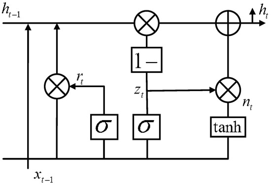
Figure 1.
Structure of GRU Network.
The GRU network calculation process is as follows:
- Firstly, we defined Wir, Whr, Wiz, Whz, Win, and Whn as the weight matrices for the different phases, and bir, bhr, biz, bhz, bin, and bhn were the bias terms.
- The GRU reset gate rt was introduced through the reset gate calculated using the equation:
- 3.
- The update gate zt controlled the amount of information forgotten by the hidden layer at the previous moment:
- 4.
- The hidden state ht carried the information of the current cell and passed it down to the network, and the last output value was chosen among nt and ht:
2.3. Sparse PCA
Sparse PCA solved the problem that PCA did not have a sparse constraint effect on the load in the main data direction. Cai T. et al. [26] proposed the sparse PCA method by improving the interpretability of PCA through the method of sparse main direction load. Sparse PCA is calculated as follows:
- A starts from the first k ordinary principal components V [1: p, 1:k] (p→∞);
- Given A as:
By solving the elasticity problem:
where j = 1, 2, …, k;
- 3.
- Given B as:
Calculate the singular value:
Finally, update A:
- 4.
- Repeat steps 2 and 3 above until convergence.
- 5.
- Finally, standardization:
3. Realization of Prediction Model
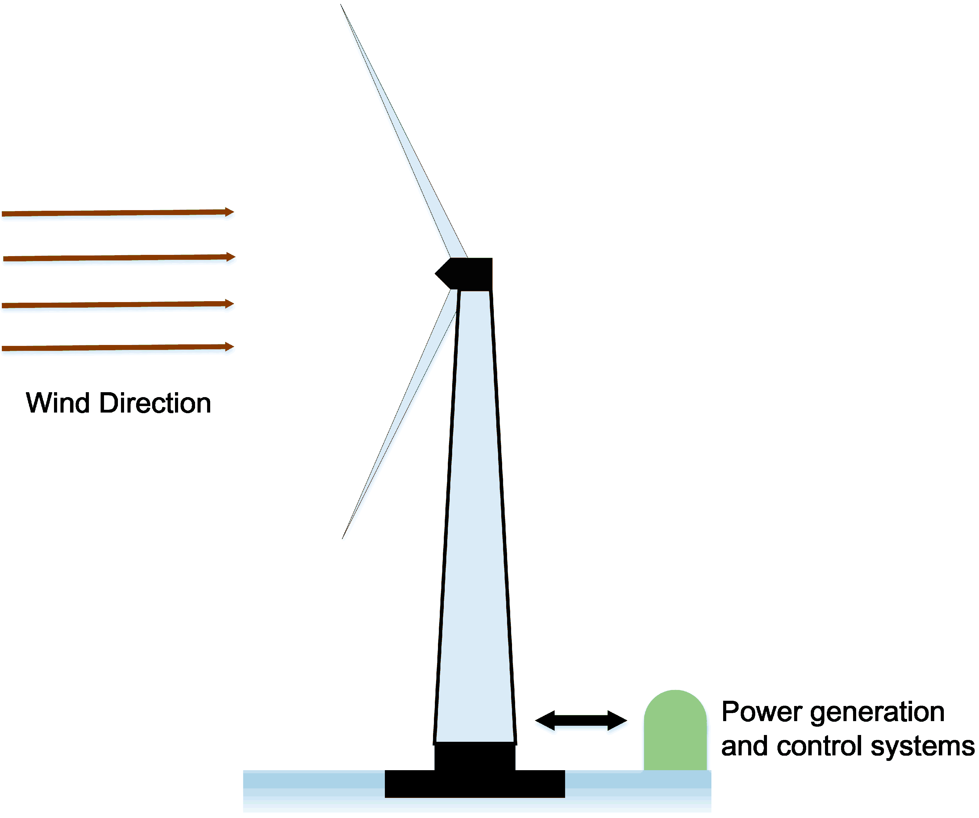
Complex weather conditions such as wind speed and direction aggravated the difficulty of wind power generation. As shown in Figure 2, the wind turbine control system timely adjusted the wind turbine according to the short-term wind speed prediction results.
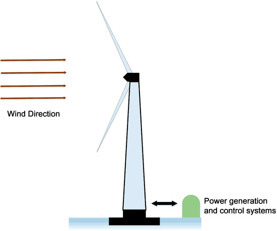
Figure 2.
Schematic diagram of wind speed prediction and control. The control system made a forecast of the next moment wind speed according to the current wind speed conditions and adjusted the wind turbine in time.
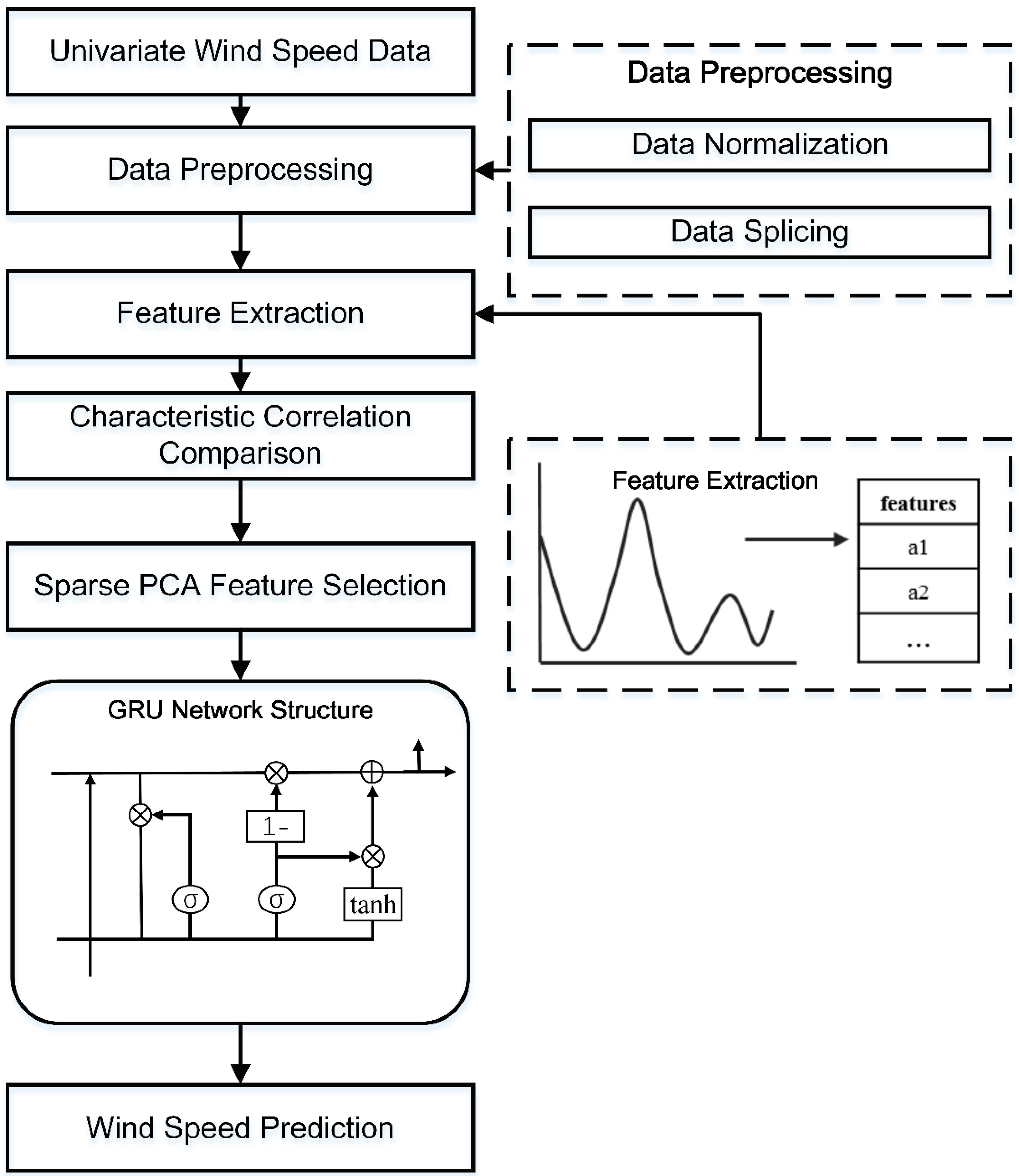
The core of the proposed hybrid model was to create feature data similar to other meteorological features, select appropriate features, and predict with a GRU network. The block diagram of the prediction method is shown in Figure 3.
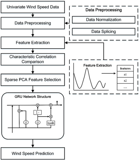
Figure 3.
Flow chart of the prediction method framework. The hybrid model preprocessed the original univariate wind speed time series data, and the processing included data normalization and data binning. Feature processing was performed on the data, including feature extraction and feature selection. Finally, all feature data were predicted using a GRU network.
The hybrid model steps were divided into the following steps:
- All data were sliced and normalized.
- Data feature processing included feature extraction and feature selection, with Tsfresh in charge of feature extraction and Sparse PCA in charge of feature selection.
- GRU accepted the input data for data fitting to obtain the predicted values and calculated the error based on the predicted and true values.
- The weights of the layers of the GRU network were updated based on the BPTT algorithm [27].
- After setting the number of training steps, steps 3 and 4 were repeated, and the Adam optimization algorithm was used to calculate the update steps until the loss function was minimized.
- After the network was trained, the wind speed was predicted for each minute of the next hour.
- Error analysis was carried out to evaluate the model performance.
During data normalization, outliers in the original data needed to be removed and the null values were filled using the average of the first seven historical data. All data were normalized using the Min-Max normalization method, as shown in Equation (14):
xi represents each value of the time series, xmax denotes the maximum value, xmin denotes the minimum value, and Xi represents the normalized value.
The normalized time series data needed to be sliced before feature extraction. The sliced data had more importance for discovering the detailed information of the time series data. The data slicing in the data preprocessing module was as shown in Figure 4. Suppose there was a set of time series. Its length is marked as “length (TimeSeriesData)”. The preprocessing module decomposed all the time series data into n copies, lt denoted the length of the subsequence, λ denoted the length of time each segment of the sequence needed to be predicted in advance, and the subsequence sliding window was δ.
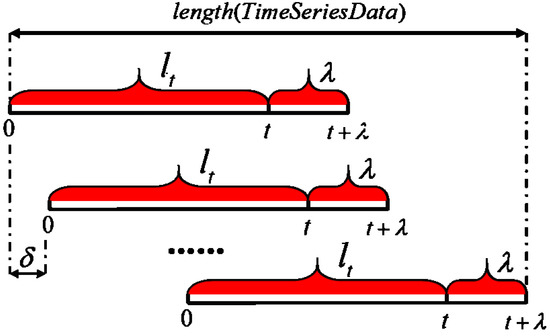
Figure 4.
Data slicing in the data pre-processing module.
The evaluation indexes for wind speed regression prediction included MAE, MSE, RMSE, and MAPE, which were calculated as shown in Equations (15)–(18):
yi denoted the true value and ŷi denoted the predicted value.
4. Case Analysis
4.1. Experimental Data
The dataset was obtained from the National Renewable Energy Laboratory (NREL). Data were readings from instruments mounted on a 270-foot weather tower with coordinates of 39°54′38.34″ N 105°14′5.28″ W. Short-term wind speed measurements were averaged from readings taken every two seconds and within one minute [28].
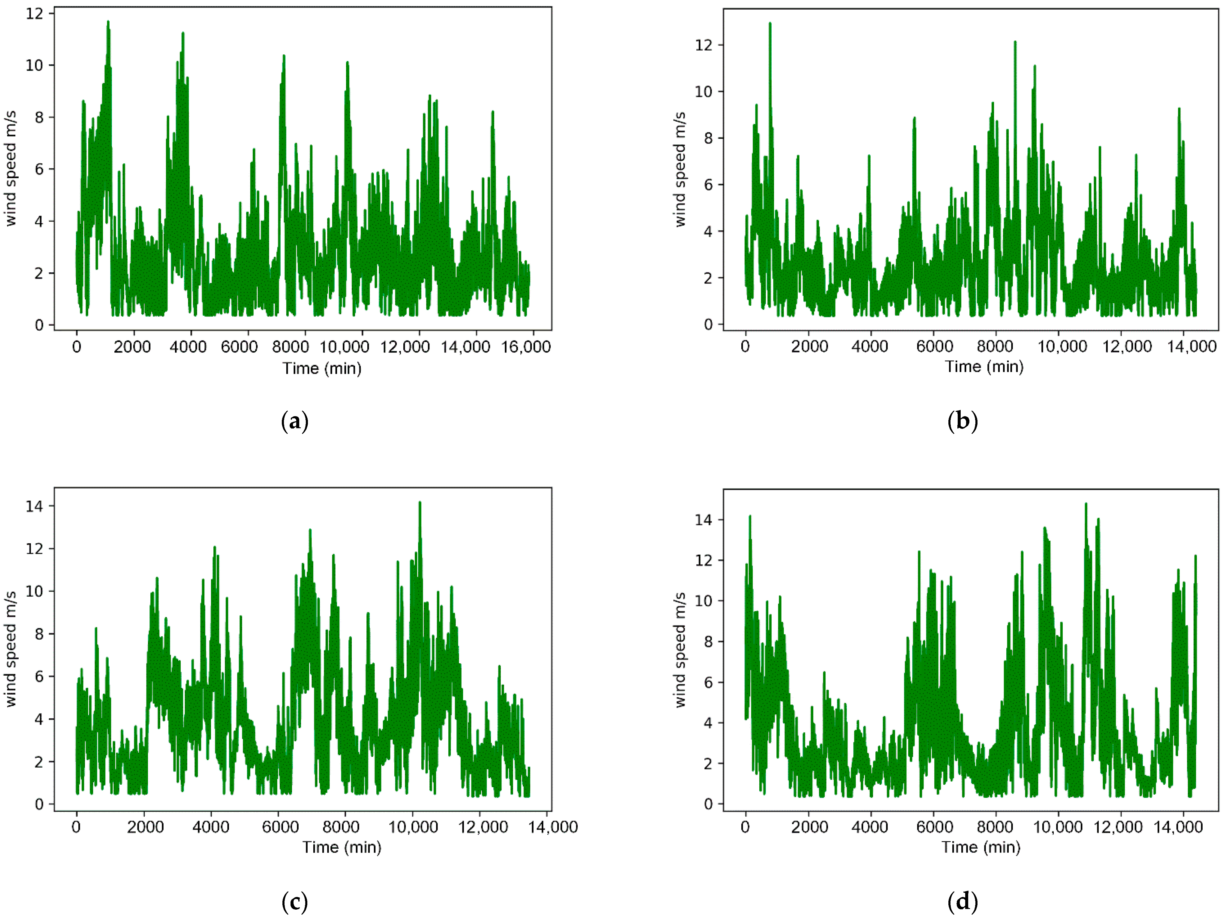
The data set for the research work in this paper was the data measured from the meteorological tower at 2 m height. The data were divided into four datasets based on the seasons, which were continuous data for ten random days in each season. The datasets had 57,600 data items, each containing wind speed data and associated with 12 other features, such as temperature, humidity, and barometric pressure. The last 60 min of data from each dataset were used for the test set, and the remaining data were divided into training and validation sets with a division ratio of 0.75:0.25. The wind speed time series of the four data sets are shown in Figure 5. The mathematical statistics of the wind speed data of each data set are shown in Table 2.
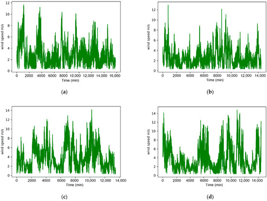
Figure 5.
Time series representation of wind speed for the four datasets. (a) Time series representation of spring wind speed dataset; (b) time series representation of summer wind speed dataset; (c) time series representation of autumn wind speed dataset; (d) time series representation of winter wind speed dataset.

Table 2.
Mathematical statistics of the four types of data.
4.2. Feature Processing Result
The feature processing work was performed only for the wind speed data of the dataset. Four datasets were subjected to feature extraction using the Tsfresh framework and feature selection was performed uniformly by Sparse PCA. Table 3 showed the number of features after feature extraction and selection for each dataset.

Table 3.
Number of feature-processed features for each data set.
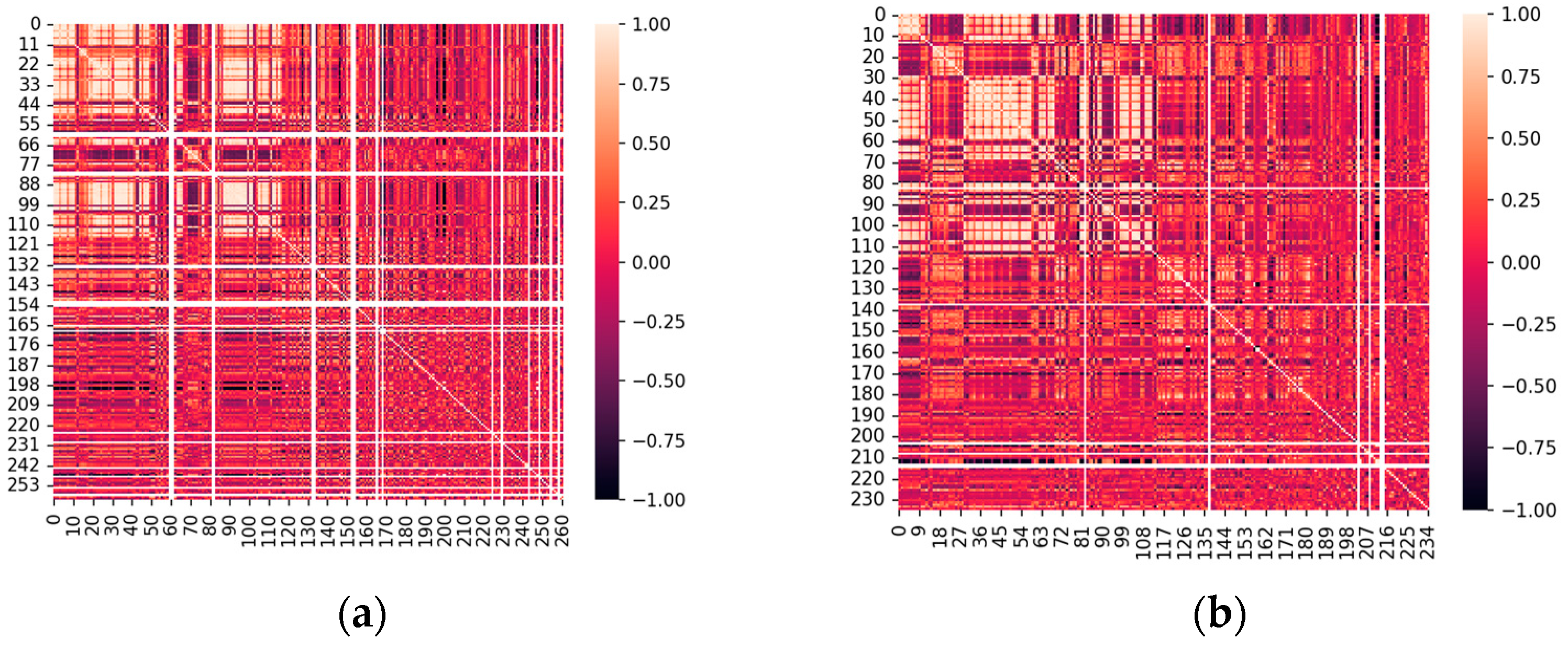
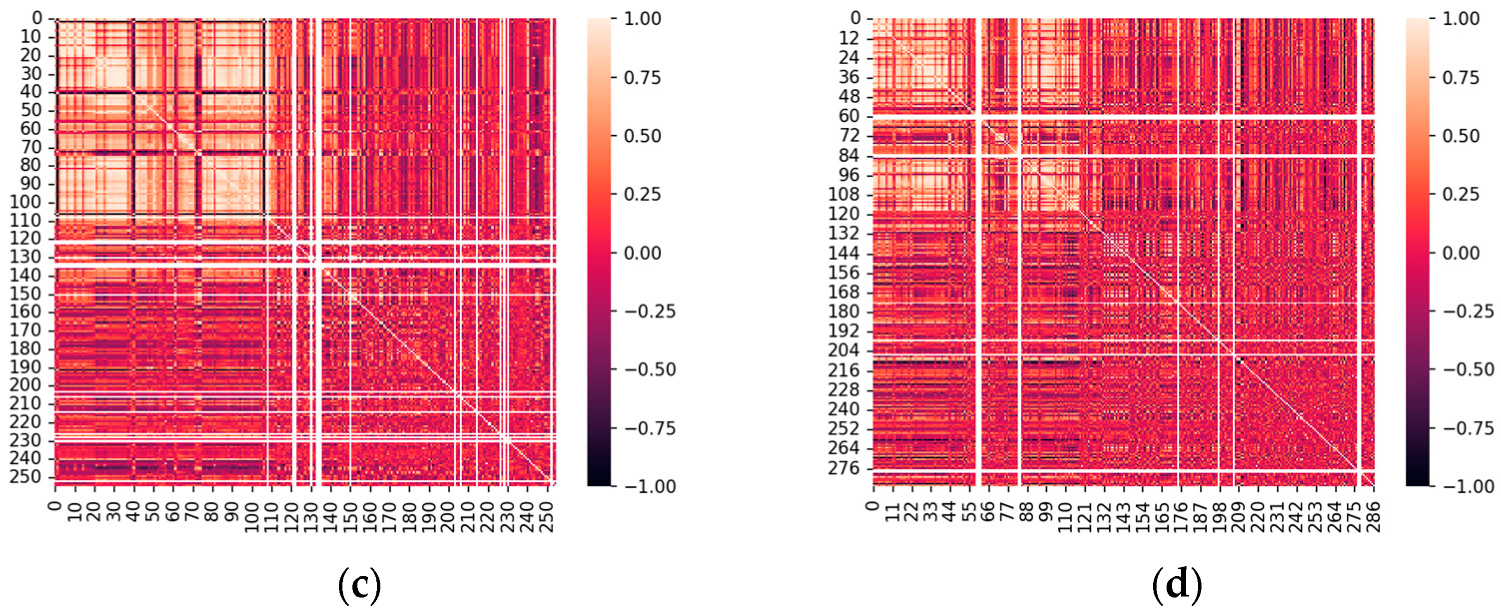
The correlation representation between the extracted features after feature processing is shown in Figure 6. The darker the color, the stronger the correlation. The figure shows that the correlation of the selected features was not high.
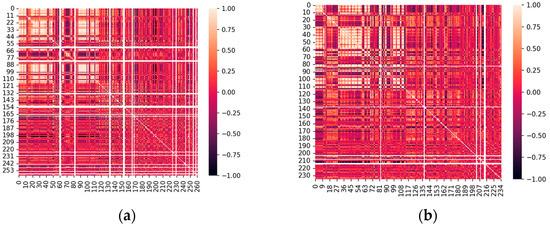
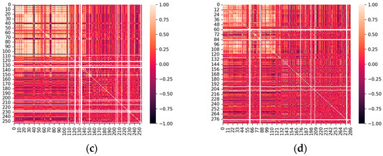
Figure 6.
Correlation of features selected for the four datasets. (a) Feature correlation representation of spring dataset; (b) feature correlation representation of summer dataset; (c) feature correlation representation of autumn dataset; (d) feature correlation representation of winter dataset.
4.3. Analysis of Hybrid Model Prediction Results
In this part, the predicted results for the four datasets are analyzed and discussed in detail.
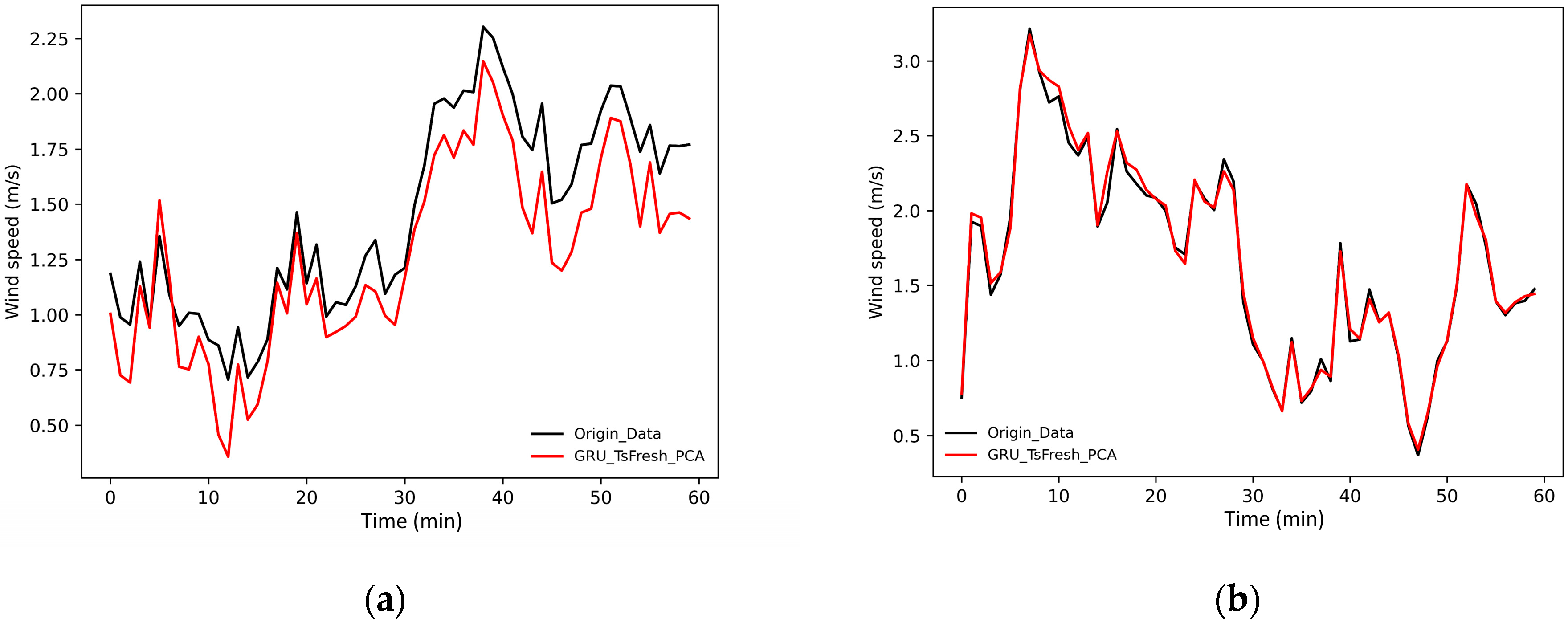
The wind speed prediction results of the hybrid model in four seasons are shown in Figure 7. The black line represents the real data and the red line represents the prediction results. The results showed that the wind speed prediction model had a good fitting trend and tracking ability, and the individual abrupt change results could not be fitted perfectly.
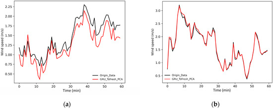
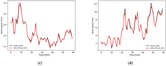
Figure 7.
Comparison of predicted and actual values for the four datasets. (a) Comparison of predicted and actual values for the spring dataset; (b) comparison of predicted and actual values for the summer dataset; (c) comparison of predicted and actual values for the autumn dataset; (d) comparison of predicted and actual values for the winter dataset.
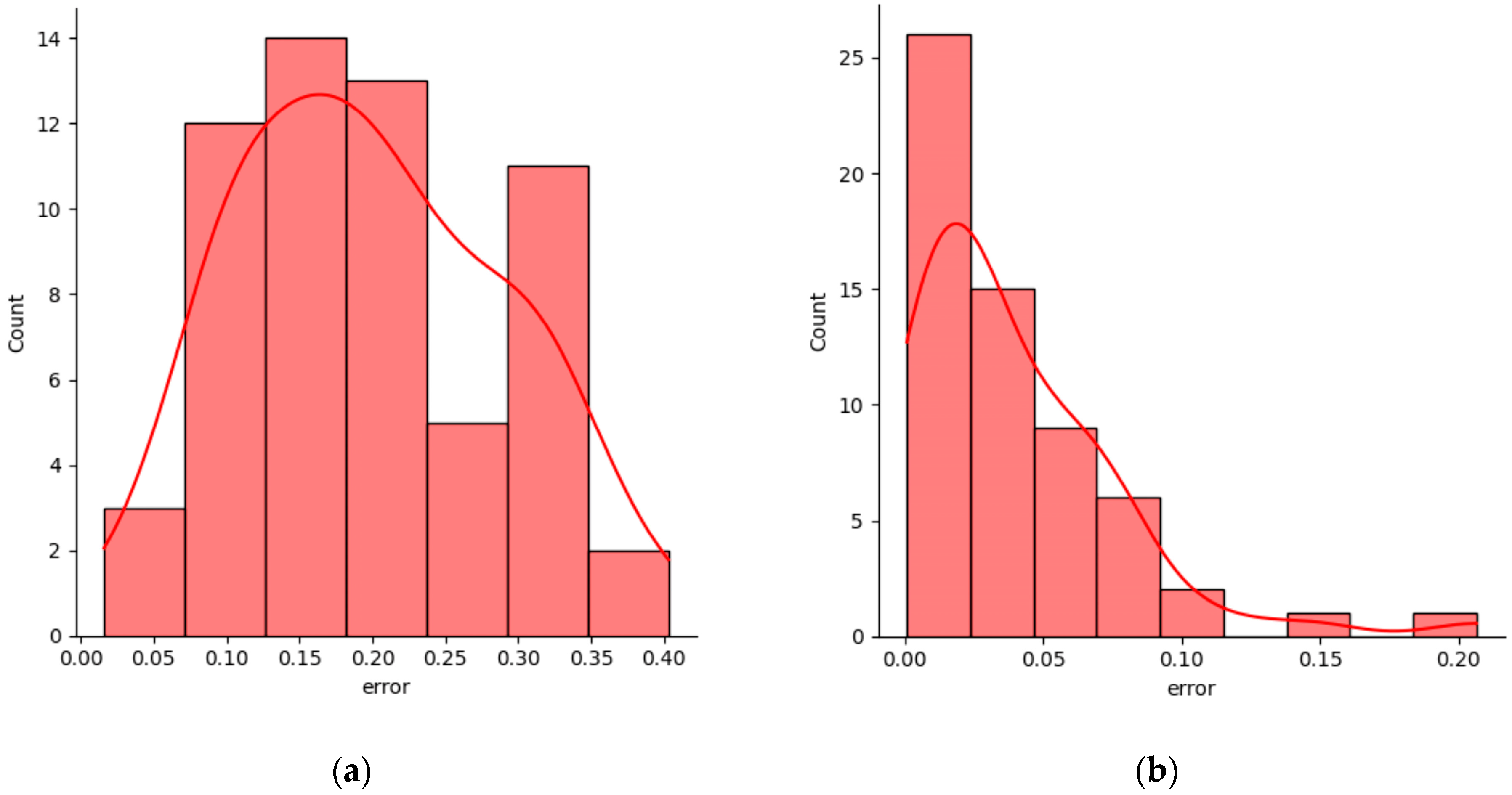
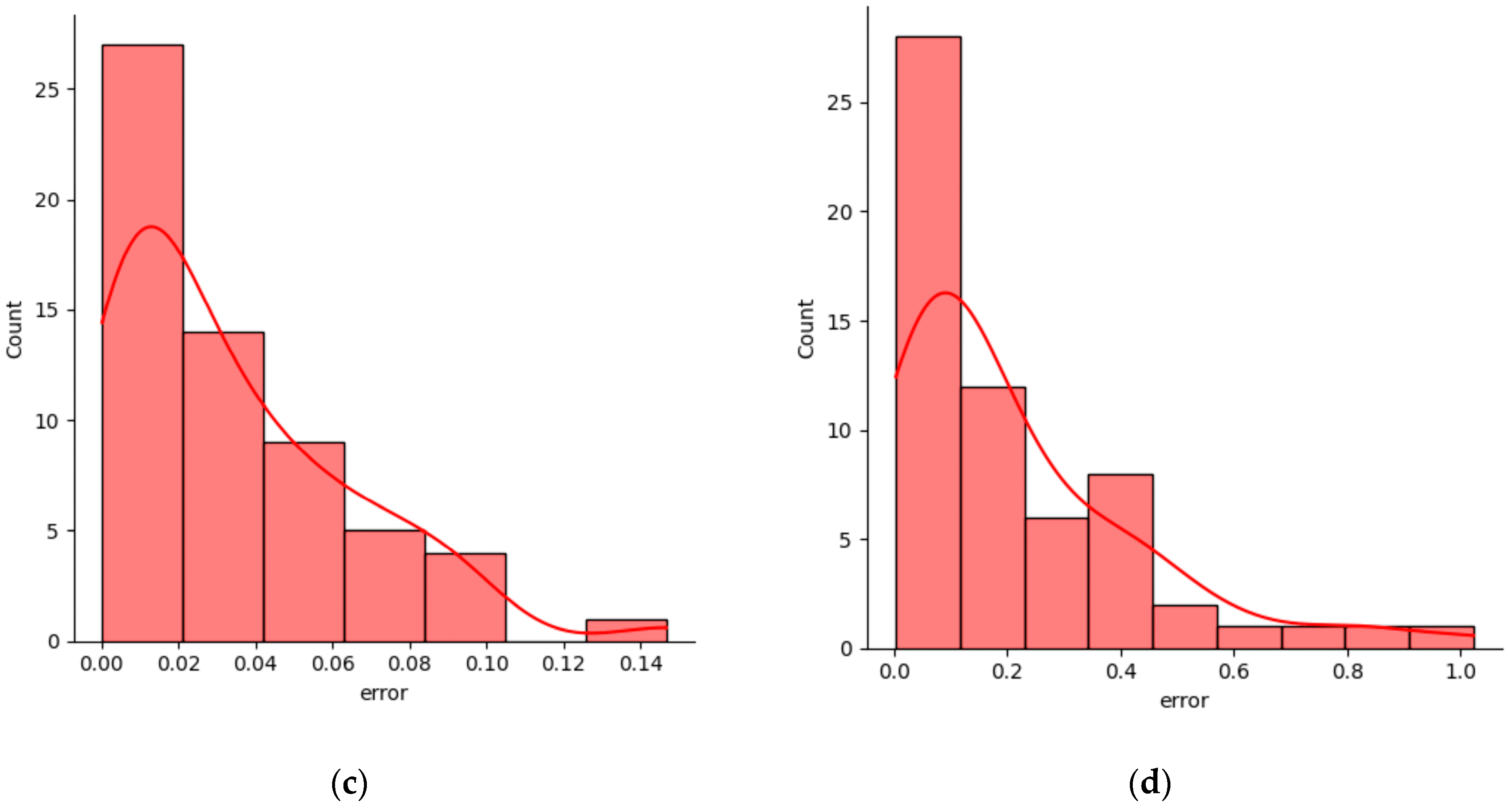
The prediction error histograms for the four seasonal data sets are shown in Figure 8. It could be seen that the maximum error was less than 1 m/s. According to the prediction evaluation index, the prediction accuracy of the hybrid model met the requirements.

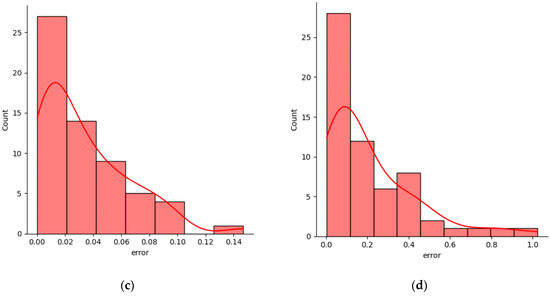
Figure 8.
Histogram of the error distribution of predicted and actual values for the four datasets. (a) Histogram of the error distribution between predicted and actual values for the spring dataset; (b) histogram of the error distribution between predicted and actual values for the summer dataset; (c) histogram of the error distribution between predicted and actual values for the autumn dataset; (d) histogram of the error distribution between predicted and actual values for the winter dataset.
4.4. Comparison of Prediction Results of Different Models
4.4.1. Description of the Control Experiment
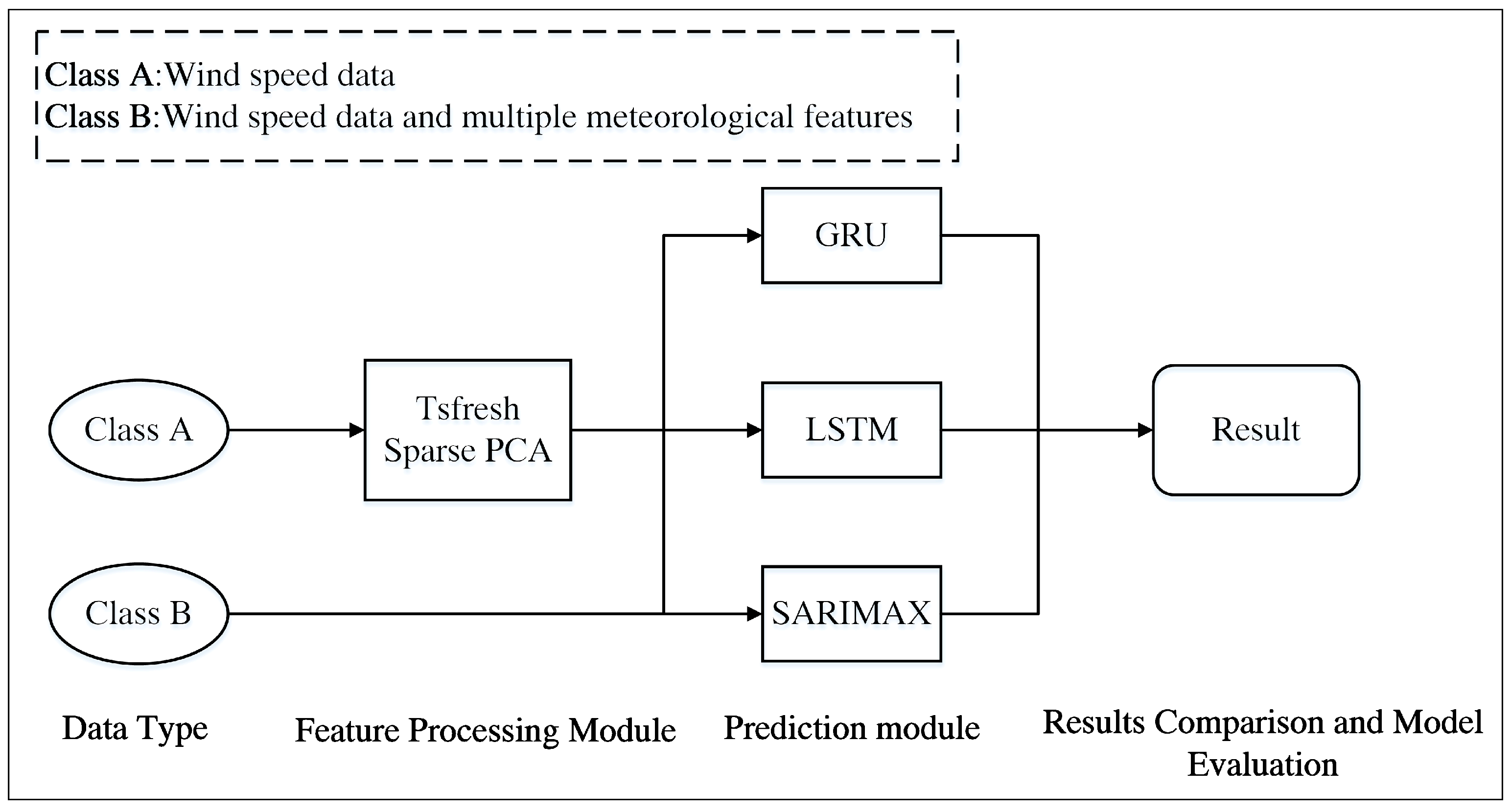
In order to measure the accuracy and feasibility of the proposed hybrid model, the SARIMAX model and the LSTM model were used as a comparison group for outcome prediction while using the same data set. The control flow is shown in Figure 9, and the module composition of the different prediction models is shown in Table 4. Each data set was divided into two data types. The first one contained only wind speed data for feature expansion, and was labeled as class A. The second one included wind speed data and 12 other relevant meteorological featured data, and was labeled as class B.
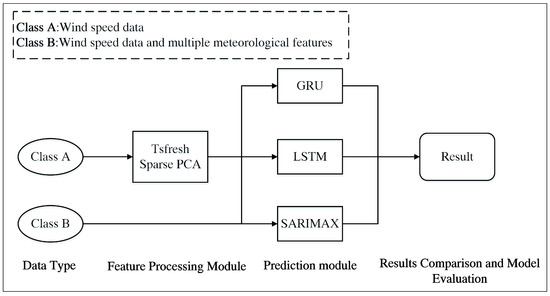
Figure 9.
Experimental flow chart between dataset and model.

Table 4.
The module composition of the different prediction models.
In terms of SARIMAX model parameter configuration, the parameters of the SARIMAX model were found by grid search to find the optimal hyperparameters. The LSTM network used a four-layer network structure, with the second and third layers being the hidden layers. The GRU network used a three-layer network structure, with the second layer being the hidden layer. GRU and LSTM networks used the same initial parameters, which included epoch, learning_rate, dropout, and activation function, etc. The hyperparameter optimization framework was used to find the optimal hyperparameters during the training phase.
4.4.2. Controlled Experimental Evaluation
In this part, the different forecasting results of all forecasting models on the four data sets are analyzed and discussed in detail. The MSE, MAE, RMSE, and MAPE metrics for all the aforementioned prediction models are shown in Table 5. The decreasing rates of the evaluation indicators obtained from the proposed model and the relevant comparison model are shown in Table 6.

Table 5.
Evaluation of the prediction results of the five models.

Table 6.
Decreasing rates of evaluation metrics of other models and the proposed model.
- (1)
- Comparing the values of the single model and neural network model on the metrics MSE, MAE, RMSE, and MAPE, it was observed that the neural network model achieved superior performance on the four metrics, which indicated that the neural network could contribute to improving the model prediction. Taking the summer dataset as an example, the MAE of the SARIMAX model was 0.57048, and the MAE of the four neural network models were 0.4237, 0.2248, 0.0492, and 0.0238, respectively. The same situation occurred for MSE, RMSE, and MAPE. Similarly, the law continued to be maintained for the other three data sets.
- (2)
- In the neural network model, the neural network with the feature extraction module performed better than the neural network model using only 12 types of climate data as feature data. Taking the summer dataset as an example, the MAE of the SARIMAX model was 0.57048, and the MAE of the four neural network models were 0.4237, 0.2248, 0.0492, and 0.0238, respectively. The same situation was observed for MSE, RMSE, and MAPE. Similarly, the law continued to be maintained for the other three data sets.
- (3)
- Among the proposed hybrid models, the GRU_Tsfresh_PCA model had better predictive power than the LSTM_Tsfresh_PCA model in the summer, autumn, and winter datasets. In the spring dataset, the prediction accuracy of the two models was the same. Taking the winter dataset as an example, the GRU_Tsfresh_PCA model decreased 17.42% in MSE, 30.42% in MAE, 9.1% in RMSE, and 1.8% in MAPE compared with the LSTM_Tsfresh_PCA model.
4.4.3. Visual Analysis of the Prediction Results
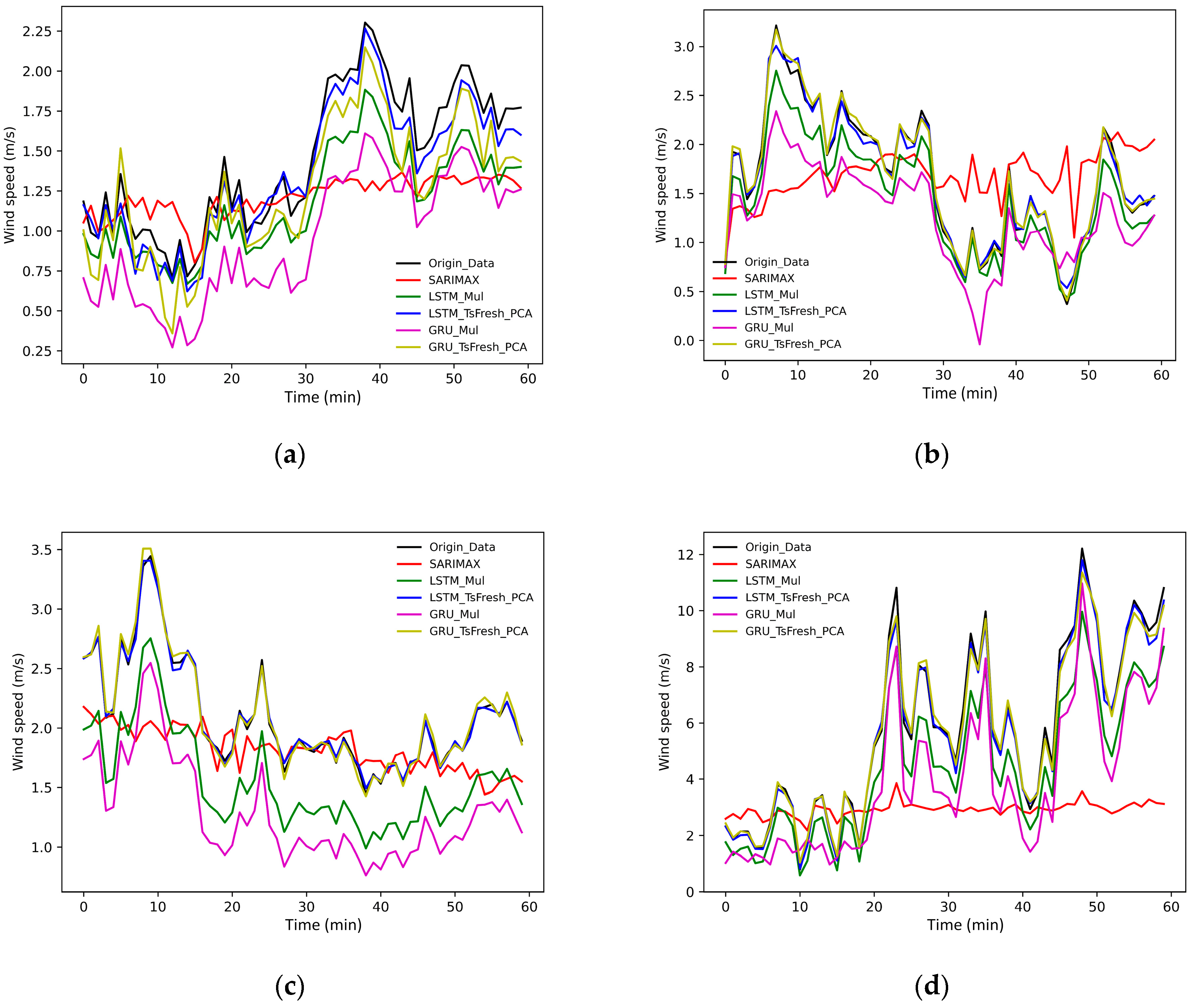
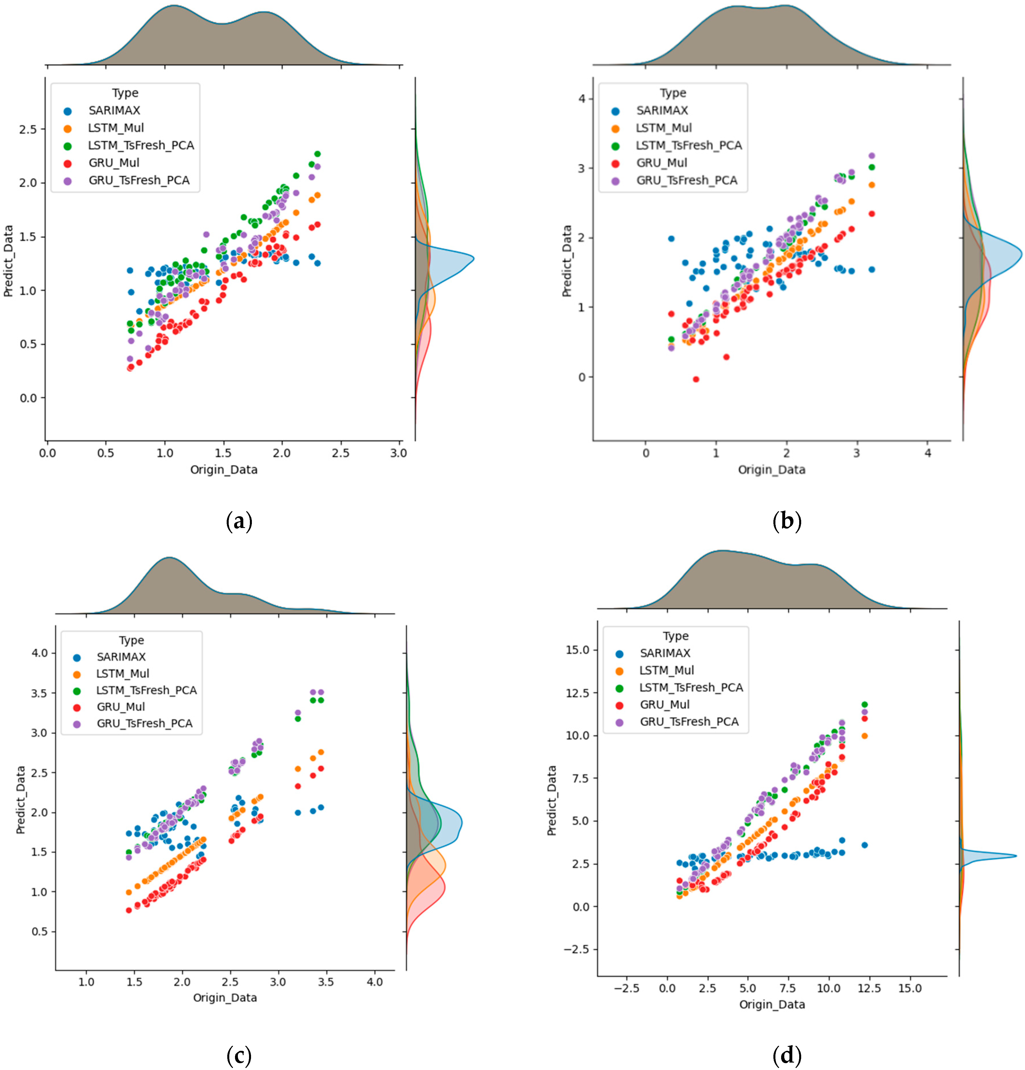
In this part, the visualization of the experimental prediction results for each of the four data sets is discussed. The comparison of prediction curves for all experimental models is shown in Figure 10. The scatter plot of the degree of fit of each model is shown in Figure 11. It can be clearly seen from Figure 10 that the fitted curves of the individual models deviated from the actual wind speed values as the prediction length kept increasing, while the prediction curves of the hybrid model based on feature extraction were relatively stable. Moreover, based on the scatter plots of different data sets, it was clearly seen that the actual wind speed prediction values of the proposed hybrid model were most evenly distributed on the regression line. Compared with other comparative models, the prediction accuracy of the proposed model did not change significantly with the change of the data set. Therefore, the predictive ability of the hybrid model was well validated.
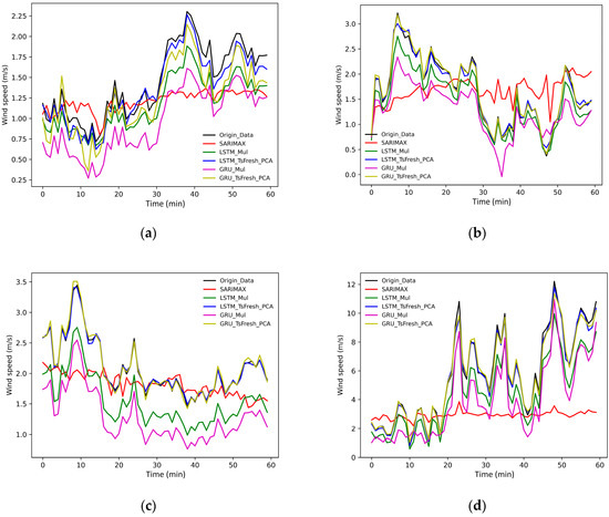
Figure 10.
Prediction results of five models. (a) Five model predictions for the spring dataset; (b) five model predictions for the summer dataset; (c) five model predictions for the autumn dataset; (d) five model predictions for the winter dataset.
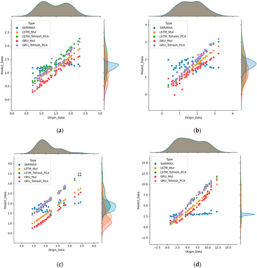
Figure 11.
Scatter plots of different model fit. (a) Scatterplot of model fit for the spring dataset; (b) scatterplot of model fit for the summer dataset; (c) scatterplot of model fit for the autumn dataset; (d) scatterplot of model fit for the winter dataset.
In addition, the evaluation metrics shown in Table 5 are visualized in Figure 12 in the form of histograms. In the same subplot, each metric for different models in different datasets was shown sequentially. Specifically, it was observed from all the prediction results that the four metrics representing the prediction performance of GRU_Tsfresh_PCA in the hybrid model were the smallest.
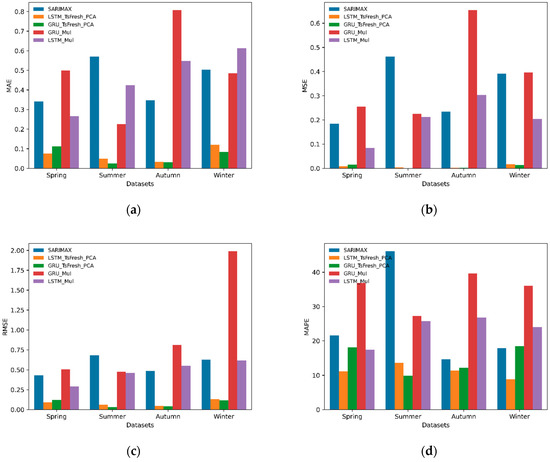
Figure 12.
Comparison of the evaluation of different models. (a) MAE comparison of different models; (b) MSE comparison of different models; (c) RMSE comparison of different models; (d) MAPE comparison of different models.
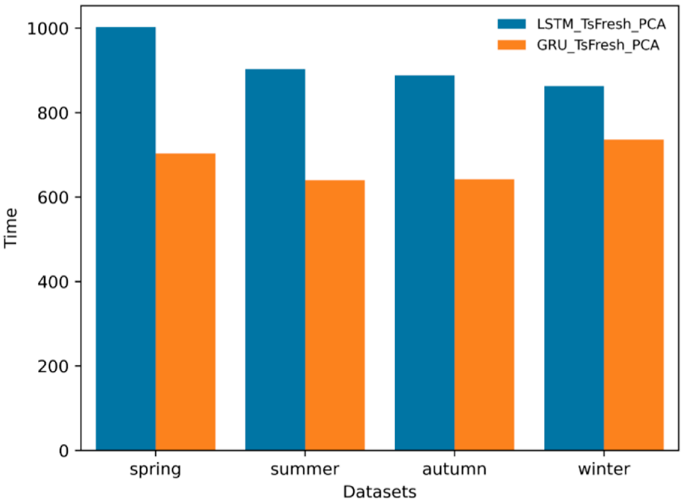
To further evaluate the performance of the LSTM_Tsfresh_PCA and GRU_Tsfresh_PCA models, the model computation times were compared under the same computational conditions, as shown in Figure 13. In addition, the starting and ending moments of time were identical. From Figure 13, it was found that the GRU_Tsfresh_PCA computation time was always lower than that of the LSTM_Tsfresh_PCA model. This meant that GRU_Tsfresh_PCA outperformed the LSTM_Tsfresh_PCA model under the same conditions.
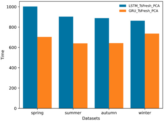
Figure 13.
Comparison of prediction time of LSTM_Tsfresh_PCA model and GRU_Tsfresh_PCA model.
5. Conclusions
For the ultra-short-term wind speed prediction problem, a hybrid prediction method based on the GRU network, sparse PCA, and Tsfresh was proposed in this paper. The model first processed the univariate wind speed data for feature extraction and feature selection. Finally, the wind speed was predicted by the GRU network. To verify the predictive ability of the proposed model, this paper performed a comparative validation using different datasets and different models, respectively. The experimental results showed that:
- (1)
- The proposed model GRU_Tsfresh_PCA had the best prediction results.
- (2)
- Experimentally, it was demonstrated that the GRU network outperformed the LSTM network under the same computational conditions after the wind speed data were processed by features.
- (3)
- The experimental results showed that the feature expansion could not only fit the existing meteorological features, but also fit the feature data more suitable for wind speed prediction than using the meteorological feature data related to the original wind speed data directly. These data were not directly obtained in reality.
- (4)
- In summary, the proposed method in this paper could be expected to have good application prospects in the future because of its low computational cost and good prediction performance.
However, there were still some limitations in this study, such as the quality of the raw wind speed data. In future research work, we will further optimize the model based on the prediction effect of the actual wind speed data to further improve the generalization ability of the model.
Author Contributions
Software, Y.W.; validation, Y.W. and R.G.; investigation, Y.W. and R.G.; data curation, Y.W.; writing—original draft preparation, Y.W.; writing—review and editing, Y.W.; visualization, Y.W.; supervision, R.G.; project administration, R.G.; funding acquisition, R.G. All authors have read and agreed to the published version of the manuscript.
Funding
This research received no external funding.
Data Availability Statement
For original wind speed data address, please visit https://midcdmz.nrel.gov/apps/sitehome.pl?site=NWTC, accessed on 5 July 2022. The processed data used to support the findings of this study are available from the corresponding author upon request.
Conflicts of Interest
The authors declare no conflict of interest.
References
- Balat, M. A review of modern wind turbine technology. Energy Sources Part A 2009, 31, 1561–1572. [Google Scholar] [CrossRef]
- Bhadane, K.V.; Ballal, M.S.; Moharil, R.M. Investigation for causes of poor power quality in grid connected wind energy-A review. In Proceedings of the 2012 Asia-Pacific Power and Energy Engineering Conference, Shanghai, China, 27–29 March 2012; IEEE: Piscataway, NJ, USA, 2012; pp. 1–6. [Google Scholar]
- Khadem, S.K.; Basu, M.; Conlon, M. Power quality in grid connected renewable energy systems: Role of custom power devices. Renew. Energy Power Qual. J. 2010, 1, 878–881. [Google Scholar] [CrossRef]
- Li, N.; He, F.; Ma, W. Wind power prediction based on extreme learning machine with kernel mean p-power error loss. Energies 2019, 12, 673. [Google Scholar] [CrossRef]
- Giebel, G.; Kariniotakis, G. Best practice in short-term forecasting—A users guide. In Proceedings of the CD-Rom Proceedings European Wind Energy Conference, London, UK, 7 May 2007. [Google Scholar]
- Aburiyana, G.; El-Hawary, M.E. An overview of forecasting techniques for load, wind and solar powers. In Proceedings of the 2017 IEEE Electrical Power and Energy Conference (EPEC), Saskatoon, SK, Canada, 22–25 October 2017; IEEE: Piscataway, NJ, USA, 2017; pp. 1–7. [Google Scholar]
- Mosaico, G.; Saviozzi, M. A hybrid methodology for the day-ahead PV forecasting exploiting a Clear Sky Model or Artificial Neural Networks. In Proceedings of the IEEE EUROCON 2019—18th International Conference on Smart Technologies, Novi Sad, Serbia, 1–4 July 2019; IEEE: Piscataway, NJ, USA, 2019; pp. 1–6. [Google Scholar]
- Chen, J.F.; Wang, W.M.; Huang, C.M. Analysis of an adaptive time-series autoregressive moving-average (ARMA) model for short-term load forecasting. Electr. Power Syst. Res. 1995, 34, 187–196. [Google Scholar] [CrossRef]
- Jeong, K.; Koo, C.; Hong, T. An estimation model for determining the annual energy cost budget in educational facilities using SARIMA (seasonal autoregressive integrated moving average) and ANN (artificial neural network). Energy 2014, 71, 71–79. [Google Scholar] [CrossRef]
- Tyass, I.; Bellat, A.; Raihani, A.; Mansouri, K.; Khalili, T. Wind Speed Prediction Based on Seasonal ARIMA model. E3S Web Conf. EDP Sci. 2022, 336, 00034. [Google Scholar] [CrossRef]
- Kritharas, P. Developing a SARIMAX Model for Monthly Wind Speed Forecasting in the UK. Ph.D. Thesis, Loughborough University, Loughborough, UK, 2014. [Google Scholar]
- Lydia, M.; Kumar, S.S.; Selvakumar, A.I.; Kumar, G.E.P. Linear and non-linear autoregressive models for short-term wind speed forecasting. Energy Convers. Manag. 2016, 112, 115–124. [Google Scholar] [CrossRef]
- Duan, J.; Zuo, H.; Bai, Y.; Duan, J.; Chang, M.; Chen, B. Short-term wind speed forecasting using recurrent neural networks with error correction. Energy 2021, 217, 119397. [Google Scholar] [CrossRef]
- Albawi, S.; Mohammed, T.A.; Al-Zawi, S. Understanding of a convolutional neural network. In Proceedings of the 2017 International Conference on Engineering and Technology (ICET), Antalya, Turkey, 21–23 August 2017; IEEE: Piscataway, NJ, USA, 2017; pp. 1–6. [Google Scholar]
- Zhu, Q.; Chen, J.; Shi, D.; Zhu, L.; Bai, X.; Duan, X.; Liu, Y. Learning temporal and spatial correlations jointly: A unified framework for wind speed prediction. IEEE Trans. Sustain. Energy 2019, 11, 509–523. [Google Scholar] [CrossRef]
- Liu, M.; Qiu, P.; Wei, K. Research on wind speed prediction of wind power system based on GRU deep learning. In Proceedings of the 2019 IEEE 3rd Conference on Energy Internet and Energy System Integration (EI2), Changsha, China, 8–10 November 2019; IEEE: Piscataway, NJ, USA, 2019; pp. 1699–1703. [Google Scholar]
- Li, C.; Tang, G.; Xue, X.; Saeed, A.; Hu, X. Short-term wind speed interval prediction based on ensemble GRU model. IEEE Trans. Sustain. Energy 2019, 11, 1370–1380. [Google Scholar] [CrossRef]
- Wu, Z.; Huang, N.E. Ensemble empirical mode decomposition: A noise-assisted data analysis method. Adv. Adapt. Data Anal. 2009, 1, 1–41. [Google Scholar] [CrossRef]
- Zhou, B.; Liu, C.; Li, J.; Sun, B.; Yang, J.; Arpino, F. A hybrid method for ultrashort-term wind power prediction considering meteorological features and seasonal information. Math. Probl. Eng. 2020, 2020, 1795486. [Google Scholar] [CrossRef]
- Jung, J.; Broadwater, R.P. Current status and future advances for wind speed and power forecasting. Renew. Sustain. Energy Rev. 2014, 31, 762–777. [Google Scholar] [CrossRef]
- Tang, J.; Alelyani, S.; Liu, H. Feature selection for classification: A review. In Data Classification: Algorithms and Applications; Chapman and Hall: New York, NY, USA, 2014; p. 37. [Google Scholar] [CrossRef]
- Chandrashekar, G.; Sahin, F. A survey on feature selection methods. Comput. Electr. Eng. 2014, 40, 16–28. [Google Scholar] [CrossRef]
- Christ, M.; Braun, N.; Neuffer, J.; Kempa-Liehr, A.W. Time series feature extraction on basis of scalable hypothesis tests (Tsfresh—A python package). Neurocomputing 2018, 307, 72–77. [Google Scholar] [CrossRef]
- Zhou, G.B.; Wu, J.; Zhang, C.L.; Zhou, Z.H. Minimal gated unit for recurrent neural networks. Int. J. Autom. Comput. 2016, 13, 226–234. [Google Scholar] [CrossRef]
- Rana, R. Gated recurrent unit (GRU) for emotion classification from noisy speech. arXiv 2016, arXiv:1612.07778. [Google Scholar]
- Cai, T.T.; Ma, Z.; Wu, Y. Sparse PCA: Optimal rates and adaptive estimation. Ann. Stat. 2013, 41, 3074–3110. [Google Scholar] [CrossRef]
- Guo, J. Backpropagation through Time, Harbin Institute of Technology: Harbin, China, 2013; Volume 40, 1–6, unpublished work.
- Jager, D.; Andreas, A. NREL National Wind Technology Center (NWTC): M2 Tower; Boulder, Colorado (Data); National Renewable Energy Lab. (NREL): Golden, CO, USA, 1996.
Publisher’s Note: MDPI stays neutral with regard to jurisdictional claims in published maps and institutional affiliations. |
© 2022 by the authors. Licensee MDPI, Basel, Switzerland. This article is an open access article distributed under the terms and conditions of the Creative Commons Attribution (CC BY) license (https://creativecommons.org/licenses/by/4.0/).


