Abstract
Demand-side management (DSM) includes various persuasive measures to improve the use of energy; thus, it has been studied from various perspectives in the literature. Nowadays, the context of productivity has an important role in the evaluation of the electrical energy systems. Accordingly, this paper presents a platform to comprehensively contemplate the DSM from the productivity perspective that features its three aspects. First, the widespread indices of DSM are manifestly redefined, and a plenary index of DSM is introduced, reflecting both energy and investment productivity. Second, the modification of energy efficacy and consumption pattern is discussed, considering a general categorization of DSM modalities based on the pertaining index of each branch. Third, a modified model of demand response (DR) is developed to implement seven DR strategies in the smart microgrids. The simulation results demonstrate that the load factor can improve up to 8.12% with respect to the normal consumption pattern. Moreover, the load factor can be further enhanced at least by 4.22% in comparison with the customary model.
1. Introduction
1.1. A Glimpse into Demand-Side Management (DSM)
DSM is mainly known as an energy-management technique that is employed to improve the consumption pattern of customers in the electrical energy systems [1]. From the energy-system point of view, the DSM can be defined as the implementation of appropriate managerial measures to influence the load-demand characteristics that make the resources on the demand side. Although the DSM refers to various persuasive measures on the demand side, the desirable modification of the load-demand characteristics via DSM improves the energy expenditure from input to consumption that causes the low carbon transition, improvement of the investment productivity, cost reductions, and a greater flexibility for the end-use consumers [2,3]. The resources caused by the DSM programs can be integrated into energy-resource-allocation frameworks or applied for regulating the investment productivity. Accordingly, the concept of DSM implies a correlation between the supply side and demand side that brings about interactive avail [4]. Moreover, the DSM is a key aspect in a smarter energy future to make accurate control over energy service, as well as affordable power utilization. The smart grids facilitate the designing and implementation of the distributed DSM schemes [5,6]. The implementation of DSM in smart grids provides a type of standing reserve that can improve the system’s operation via the adjustment of renewable resources’ dispatch [7]. The advantages of DSM are enumerated in Table 1.

Table 1.
Capabilities and advantages of DSM implementation.
1.2. DSM Strategies
Mainly, the DSM includes many diversified strategies [44,45,46]. The overall demand reductions, along with demand response (DR), were expressed as two general strategies of DSM in Reference [47]. The strategies of DSM are adopted according to the size of electricity grid and energy consumption, technological infrastructure, circumstance of interaction between implementer and participants, deregulation characteristics, and the potential of different load-demand types. The use of efficient appliances and lights, commercial load scheduling, restricting residential appliance use, price incentives, and tariff structure, as well as community involvement, consumer education, and local committees for the mini-grids, was enumerated in Reference [48] as the applicable strategy of DSM. In the active distribution grids, energy efficiency, orderly power utilization, and DR are the primary strategies [49]. In the widespread classification of the DR, time-based (price-based) programs and incentive-based programs are two general categories [50,51]. The time-based programs are based on price-driven strategies. The price-driven DR was studied in Reference [52], where the electricity price signals were used to influence the customers’ energy consumption pattern. The effects of price-based and incentive-based DR strategies on the operational cost reduction of a microgrid were scrutinized in Reference [53]. The load-shifting mechanism as a type of orderly power-utilization strategy was focused on in the design of a trilevel energy market model in Reference [54] that was implemented via a time-of-use (TOU) pricing scheme.
1.3. Role of DSM in Energy Management
Practically, the DSM is a main constituent of energy-management frameworks in the smart grids. A game theoretic DSM model for distributed energy management was proposed in Reference [55] to incorporate the energy-storage components while taking into account the supply constraints in the form of power outages that employ emerging blockchain technologies. An optimization model of energy scheduling was suggested in Reference [15] for the microgrids, including responsive loads that adopts the TOU and real-time pricing (RTP) strategies. The application of solitary TOU tariffs has been found to be suitable for long-term modification of the load curve [56]. The solitary RTP strategy was implemented in Reference [57], underlying a Stackelberg-game approach. The RTP strategy for peak load shaving was adopted in Reference [58], such that the reduced load demand can diminish the spinning reserve required for dealing with the uncertainties of renewable resources during the peak load periods, whereas more renewable power outputs can be allocated to the increased load demand during the off-peak load periods. The dynamic pricing strategy in price-based DR is significantly efficient in the smart grids [37,38,39]. A model for optimal scheduling of microgrids was proposed in Reference [59], where an incentive-based DR strategy was pursued by considering the load, price, and renewable-energy uncertainties. The concept of online DSM was studied in Reference [60]; it considers an internal RTP strategy of a microgrid by using a combination of supply–demand mismatch power and inclining block rate mechanism to optimize the load profile. The interruptible/curtailable strategy was used in Reference [61] for optimal market-based microgrid operation. The different DSM programs may be implemented simultaneously. An energy-management framework for optimal operation of grid-connected microgrids was developed by Reference [62] that pursues the flexible load-shaping DSM strategy, as well as price-based and incentive-based DR strategies in the presence of non-dispatchable energy resources.
1.4. Motivation, Needs, and Aims
There are several noticeable review papers in the DSM arena. Some of the papers have focused on the flexibility. The electricity grid flexibility solutions for the insular scope via DSM and storage were discussed in Reference [63]. The power flexibility and joint power-heat flexibility potentials in energy-intensive industries were investigated in Reference [64], considering DR programs. Two important features of the existing review papers are the DSM methods’ classification and the scope of discussion. A comparison of the present work and some previous reviews is presented in Table 2.
Table 2.
Comparison of present work and some previous reviews in the DSM arena.
Since the productivity is considered as a fundamental pillar for the evaluation of energy systems, the energy productivity and the pertaining monetary contexts are crucial themes in the DSM [70,71]. Accordingly, this paper tends toward reconsideration of DSM contexts from the productivity perspective. This issue requires the development of a general index for the DSM index by considering the energy efficiencies, the asset productivity, and the investment thrift in the electrical energy system to analyze and model the DSM modalities. Since the most important modality of DSM in the smart grids is DR, a modified DR model is presented so that value of the developed general index for DSM can be enhanced due to the rational payment criteria embedded in the model that determines the incentives and penalties by considering the real-time reaction of the customers regarding electrical energy consumption.
2. DSM Indices
Several indices for DSM have been proposed in the literature. The load factor, peak-to-valley distance, and reduced energy consumption were used in Reference [62]. Moreover, the peak load reduction, peak-to-average ratio, and the energy cost were enumerated in Reference [72].
In order to facilitate the DSM analysis, the DSM indices need to be perspicuously organized. The precise definitions are presented in this section, and a general index is introduced for DSM analysis from the energy-management point of view, called the ‘DSM index’. Moreover, an illustrative implementation is accomplished by which the values of the indices are calculated.
2.1. Demand Factor
The demand factor is defined as the peak load demand divided by the average suppliable electrical power during a specified time span, and it can be formulated as follows:
From the energy-management perspective, the demand factor can be construed as the maximum required energy resource capacity divided by the available energy resource capacity during the time span, and it can be reformulated as follows:
If the available energy resource capacity is assumed to be constant during the time span, according to Equation (3), the length of time will be ineffectual and the demand factor can be regarded as the peak load demand divided by the maximum suppliable electrical power:
Theoretically, the value of this index is a real number between zero and one.
2.2. Utilization Factor
The utilization factor is defined as the average supplied electrical power divided by the peak load demand during a specified time span, and it can be formulated as follows:
From the energy-management perspective, this index can be construed as the supplied energy divided by the maximum required energy resource capacity, and it can be reformulated as follows:
Theoretically, the value of this index is a positive real number.
2.3. Load Factor
The load factor is an index that is widely used for load-curve analysis [73,74,75]. This index is defined as the average load consumption divided by the peak load demand during a specified time span ([62]), and it can be formulated as follows:
From the energy-management perspective, this index can be construed as the delivered energy divided by the maximum required energy resource capacity, and it is reformulated as follows ([76]):
Moreover, the load factor can be calculated by the following expression:
where is the grid efficiency. Thus, the load factor is the product of the utilization factor and the grid efficiency. Theoretically, the value of this index is a real number between zero and one. Sometimes the inverse of load factor, namely the ‘peak-to-average ratio’, is used [55].
2.4. Capacity Factor
The capacity factor is defined as the average supplied electrical power divided by the maximum suppliable electrical power during a specified time span, and it can be formulated as follows:
From the energy-management perspective, this index can be construed as the supplied energy divided by the available energy resource capacity, and it can be reformulated as follows ([76]):
Theoretically, the value of this index is a real number between zero and one.
2.5. Delivery Factor
The delivery factor is defined as the delivered energy divided by the available energy resource capacity, and it is formulated as follows:
Moreover, the capacity factor can be formulated as the following expression:
Thus, the delivery factor is the product of the capacity factor and the grid efficiency. Theoretically, the value of this index is a real number between zero and one. Moreover, the delivery factor can be reformulated as the following expression:
Thus, the delivery factor is the product of the demand factor and the load factor. Consequently, the delivery factor can be decomposed in two ways, as follows:
2.6. Regulation Factor
The regulation factor is defined as the demanded energy divided by the available energy resource capacity, and it can be formulated as follows:
Theoretically, the value of this index is a real number between zero and one for the energy-surplus situation, whereas it will become greater than one for the energy-shortage situation. The regulation factor can be used for daily power markets. If this index is considered for a real-time state, the demanded energy can be replaced by the delivered energy.
2.7. Adequacy Coefficient
This index is a function of the regulation factor, which is defined as follows:
where represents the Heaviside step function. Theoretically, this index takes a binary value. It is one for the energy-surplus situation, whereas it will be zero for the energy-shortage situation.
2.8. System Productivity
This index is defined as the adequacy coefficient multiplied by the delivered energy divided by the available energy resource capacity, and it can be formulated as follows:
Theoretically, the value of this index is a non-negative number less than one. Moreover, the system productivity can be reformulated as the following expression:
Thus, the system productivity is the product of the adequacy coefficient and the delivery factor.
2.9. Energy Productivity
The arena of energy productivity applications is extremely wide [77,78,79]. This concept has been evaluated in different countries [80,81,82]. The energy productivity can be regarded as the inverse of energy intensity that determines the value of produced services for one unit of energy used [83]. In the present paper, this index is defined as the useful energy divided by the available energy resource capacity, and it can be formulated as follows:
Theoretically, the value of this index is a real number between zero and one. The DSM index can be reformulated as the following expression:
where represents the consumption efficiency defined in Reference [66]. Thus, the energy productivity is the product of the delivery factor and the consumption efficiency.
2.10. DSM Index
This index is defined as the adequacy coefficient multiplied by the useful energy divided by the available energy resource capacity, and it can be formulated as follows:
Theoretically, this index takes a non-negative value less than one. Moreover, the DSM index can be reformulated as the following expression:
Thus, the DSM index is the product of the system productivity and the consumption efficiency. Accordingly, we obtain the following:
which means that the DSM can be evaluated by the adequacy coefficient and the energy productivity. Consequently, the DSM index can be decomposed as follows:
The relationship of the defined indices is illustrated in Figure 1. As a result, the general index of DSM is ‘DSM index’ (DSMI) that includes the energy and economical efficacious. The adequacy coefficient and the energy productivity are two factors that can completely exhibit the circumstance of DSM. Moreover, the latter can be decomposed to three components: the demand factor, the load factor, and the consumption efficiency. For instance, the specific load curves for end-use power consumption and supplied electrical power have been depicted in Figure 2. Also, the specific load curves for end-use power consumption and useful electrical power have been depicted in Figure 3. In this case:
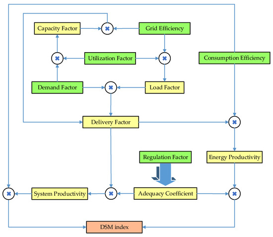
Figure 1.
The relation of the different indices for DSM.
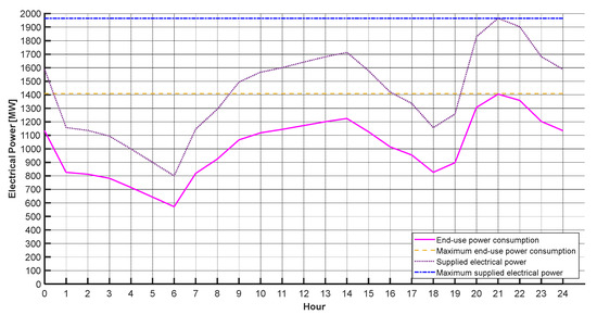
Figure 2.
The specific load curves for end-use power consumption and supplied electrical power.
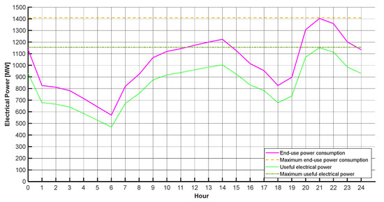
Figure 3.
The specific load curves for end-use power consumption and useful electrical power.
Therefore, we have the following:
3. Classification and Analysis of DSM
Generally, the DSM can be divided into ‘energy conservation’ and ‘electrical load management’. The energy conservation involves the adequacy coefficient for analyzing the energy consumption reduction in energy-shortage situations, and the consumption efficiency for analyzing the energy-efficiency enhancement. The energy-conservation modalities are elucidated in Table 3.
Table 3.
Analysis of energy-conservation techniques.
On the other hand, the electrical load management involves the adequacy coefficient for analyzing the energy-consumption reduction when system reliability is jeopardized, the demand factor for analyzing the demand matching, and the load factor for analyzing the load profile’s improvement. The general classification of DSM based on the index of each branch is shown in Figure 4.
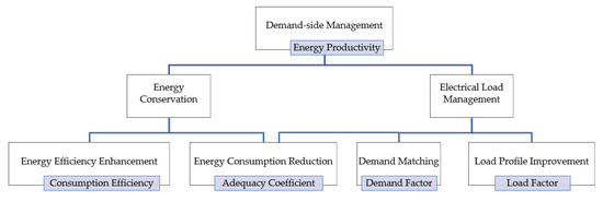
Figure 4.
The general classification of DSM based on the index of modality.
The branches are elucidated in the following.
3.1. Load Profile Improvement
The electrical load management involves the techniques of load-profile improvement based on the efficacious strategies for changing the consumption pattern via orderly mechanisms. The load-profile improvement is mainly evaluated via assessment of the load factor index [19,84,85]. There are several mechanisms for the electrical load management divided into three categories. First, strategic saving aims at energy-consumption reduction in a certain time span that includes peak clipping and strategic conservation mechanisms. The peak clipping improves the load profile considered for one hour, whereas strategic conservation improves the system productivity, and the effect of strategic conservation on the load curve is basically evaluated for 24 h. Second, strategic productivity aims at load-profile improvement under the same total energy consumption that involves load shifting and flexible load-shape mechanisms. Third, strategic transfusion aims at load-profile improvement via energy consumption increment and electrification that involves valley filling and strategic load-growth mechanisms.
The change of load factor is given by Equation (27):
In the load shifting and flexible load-shape mechanisms, the average load consumption will be unchanged. Therefore, if , the load factor will rise, but if , it will drop.
If and are two points in , the change of load factor will be given by the following:
It is assumed that the changed load curve is described as follows:
Hence, the change of load factor can be obtained as follows:
This shows that if , the change-of-load factor will be positive. This means the following:
- If the local peak clipping occurs in the peak load periods, the load factor will improve,
- If the load consumption is added in off-peak load periods but does not exceed from the old peak, the load factor will improve.
Moreover, considering the linear piecewise load curve that reflects the average load consumption for each hour, it can be concluded that if the load consumption is added in all periods and exceeds from the old peak, the load factor will diminish.
Now, it is assumed that the changed load curve is described follows:
Hence, the change of load factor can be obtained as follows:
This shows that if , the change of load factor will become negative. This is because of the following:
This means that if the load-consumption reduction occurs in the off-peak load periods, the load factor will diminish.
Considering the stepwise function approximation of the load curve, the following procedure is applicable:
It shows that, if the load consumption reduction occurs in the off-peak load periods, the load factor will diminish; this is because the right-hand side is reduced.
From the above expressions, it can be concluded that the load-demand reduction in peak load hours and the limited load-consumption increase in off-peak load periods are desirable in the load-management techniques.
Now, it is assumed that the changed load curve is described as follows:
where is a real number. It results in the following:
Considering Equation (27), if , the load factor will improve, and if , the load factor will diminish. In other words, the strategic load growth will correct the load curve, whereas the strategic conservation will deteriorate the load factor. Therefore, the effect of strategic conservation needs to be captured by a different index called adequacy coefficient that is described afterward. It is worth mentioning that the changed load curve is described as follows:
where k is a positive real number. Moreover, the same result will be obtained because of the following:
3.2. Demand Matching
The demand matching refers to the coordination of the required energy resource to satisfy the load demand and the available energy resources. The demand factor is a suitable index for demand matching. In order to show the role of demand matching, two cases are supposed to have the same corrected load curve, as depicted in Figure 5. Thus, the load factors of the two cases are equal. If the strategic conservation is not required for both cases (i.e., the adequacy coefficient is equal to one and the peak load demand does not exceed from the available energy resource capacity for both cases), the load management is more effective for that case in which the available energy resource is less than the other. In other words, although the load factors are equal, the demand factor of case 2 is better according to (2). Hence, the effective load management supplementally needs to a load growth strategy in the case 1 to match the load demand with the available energy resource capacity.
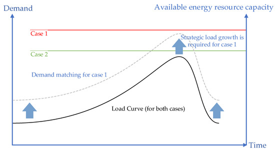
Figure 5.
The demand-matching concept.
3.3. Energy-Consumption Reduction
The energy-consumption reduction includes the decrease of terminal energy of end-use customers, as well as strategic conservation. Mostly, the decrease of terminal energy is a result of energy audit modality [86,87,88]. Therefore, the consumption efficiency improves and the energy productivity is enhanced according to Equation (24). On the other hand, from the load-management viewpoint, if the energy shortage occurs, the strategic conservation will be required. In such conditions (shown in Figure 6), the adequacy coefficient is equal to zero because the value of the regulation factor is greater than one; thus, the DSMI is equal to zero. Although strategic conservation deteriorates the load factor, this action is required so that the actual energy productivity can be improved.
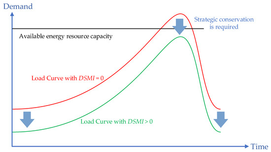
Figure 6.
Role of adequacy coefficient in reflection of strategic-conservation necessity in DSM index.
3.4. Energy-Efficiency Enhancement
The energy-efficiency enhancement correlates with the economic issues and environmental concerns [89]. The energy-efficiency investments should be scrutinized to estimate the success of pertaining DSM programs that aim toward electricity-efficiency enhancement [90]. The enhancement of consumption efficiency is feasible via the energy recovery (see Reference [80], for example) and the energy audit (see References [91,92], for example). The efficiency indicators for urban energy systems, including thermodynamic indicators, physical indicators, physical–thermodynamic indicators, economic–thermodynamic indicators, and economic indicators, were used in Reference [93].
4. Comprehensive Model of DR
The DR is the most important modality of electrical load management. Generally, the energy balance of the smart grids can be achieved by implementation of DR. The investigations in the DR arena lack the extensive model by which the prevalent methods can be described distinctly. Moreover, the previous models have mostly focused on the reduction of energy consumption in different time periods, whereas the smart grids provide a useful groundwork to pay attention to energy efficiency from the operator’s point of view, even in short-term and medium-term time horizons. One of the neglected concepts is the load augment in off-peak load periods to improve the energy efficiency of the power system. This section develops an analytic framework for elucidating the load augment in the prevalent DR strategies. To attain this goal, a comprehensive mathematical model for DR is presented considering the different coefficients that specify a prevalent method and the mutual effect of load and the motivational factors. The most common strategies, including seven DR strategies, are simulated in the short-term time horizon. Then the effect of the electrification is investigated in the seasonal load profile. The simulation results demonstrate the improvement of smart grid operation by electrification.
The classic economic model of elastic loads was organized in References [94,95,96]. The weighting coefficient that was used in Reference [97] was embedded into the DR model to take into account the customers’ reaction in response to the implementation of price-based and incentive-based DR programs. The nonlinear DR models were formulated in Reference [98] based on the concept of the classic economic model of elastic loads. A modified inclusive DR model was developed in Reference [34] that uses six distinctive contexts (i.e., incentive coefficient, penalty coefficient, upfront reservation payment, threefold frame, dynamic pricing, and artificial peak) to form seven DR methods (i.e., time of use, critical peak pricing, real-time pricing, technological direct load control, voluntary response program, capacity market, and contractual indirect load control).
In this section, it is assumed that the load consumption changes from the initial quantity on the basis of the energy requirements, as well as customers’ eventual reaction to the conditions considered in the individual DR contracts:
Equation (39) states that the load demand change for the specified time period is equal to the difference between the real-time load demand and the initial load demand value at that time period.
Although the reactions are impressed by the electricity prices, the quantity of demand can be considered as an independent variable in derivation [94,95,98]. Thus, the change of the electricity price for single-period analysis can be formulated as follows:
Equation (40) states that the electricity price change for the specified time period is equal to the difference between the real-time electricity price and initial electricity price at that time period. For multi-period analysis, the electricity price change for a specified time period is regarded as a function of all time periods. The relation between load demand and electricity price is given by , inclusively [98].
The analysis involves two distinct time periods on the basis of the normal consumption pattern. In order to distinguish the peak load periods and the off-peak load periods, a distinction factor is defined as follows:
For each type of time period, two payments are assigned: payment for change (PFC) and payment for deviation (PFD). The PFC can be an incentive or penalty, but the PFD is always in the form of a penalty. The calculations of these payments are performed on the basis of the new state of the load demand. For each type of time period, three bands are determined: compensative, permissive, and forbidden bands:
- In the permissive band, an incentive is assigned for efficacious change of load demand (curtailment of load demand for peak load periods and augment of load demand for off-peak load periods). Moreover, a penalty is assigned on based on the value of breach.
- In the compensative band, a fixed incentive was assigned for the efficacious change of load demand (curtailment of load demand for peak load periods and augment of load demand for off-peak load periods). Moreover, a fixed out-of-domain penalty was assigned based on the value of the specified contracted level.
- In the forbidden band, three penalties were determined. The first penalty was assigned to an inappropriate change of load demand (curtailment of load demand for off-peak load periods and augment of load demand for peak load periods). The second penalty was based on the value of breach. The third penalty was assigned to the forbidden load consumption state.
Afterward, the payments for the peak load periods and the off-peak load periods were elucidated.
4.1. Payment for Peak Load Periods
The functions of penalties and incentives for peak load periods were determined and are presented in Figure 7.
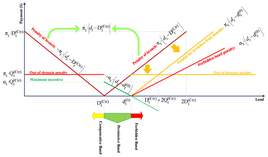
Figure 7.
Functions of penalties and incentives for a typical peak load period.
The PFC is calculated as follows:
where represents the unit ramp function. The PFD is calculated as follows:
As Figure 7 shows, the penalty of breach can be further categorized as out-of-domain penalty and the penalty for deviation from domain. Thus, the total payment is obtained as follows:
The quantity of payment rates (incentives or penalties) can be derived from the difference between the microgrid profit before implementing the DR program and its primary projected benefit [99]. The optimal values of the parameters determined in the contracts can be obtained by the approach suggested by Reference [100].
4.2. Payment for off-Peak Load Periods
The functions of penalties and incentives for the off-peak load periods were determined and are presented in Figure 8.
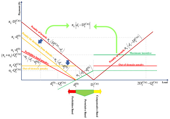
Figure 8.
Functions of penalties and incentives for a typical off-peak load period.
The PFC is calculated as follows:
Moreover, the PFD is calculated as follows:
As Figure 8 shows, for forbidden band the penalty of breach can be decomposed into the out-of-domain penalty and the penalty for deviation from domain. Thus, the total payment is obtained as follows:
4.3. Individual Payments for Each Band
Figure 9 shows the characteristic of individual payments for each band.
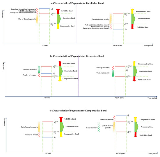
Figure 9.
Characteristics of individual payments for each band.
4.4. Unified Function for Total Payment
The unified function of total payment for all periods is given by the following equation:
Generally, the payments can be determined as follows:
Completely, Table 4 shows the comprehensive overview of payments. Therefore, the final payment is given by the following equation:
Table 4.
Comprehensive overview of payments.
The Model of DR is developed for elastic loads, using Equation (50).
4.5. Model of DR for Elastic Loads
First, it is assumed that is the total income of customers during time horizon (T) due to the power utilization; thus, the customers’ net profit will be as follows:
4.5.1. Model of Single-Period DR for Elastic Loads
For the single-period modeling, the value of power utilization is considered as the function of conditions in a specified time period that only depends on the electricity price of that time period. Hence, only the self-elasticity emerges in the equations.
According to the optimization framework, in order to maximize the customers’ profit, the derivation of the right-hand side of (51) must result in zero; therefore, we obtain the following equation:
Consequently, we obtain the following:
and,
The Tylor expansion of the customers’ net profit function will result in the following:
Therefore, we obtain the following:
Consequently, we have the following:
4.5.2. Model of Multi-Period DR for Elastic Loads
For the multi-period modeling, the value of power utilization is considered as the function of electricity price in all time periods. Hence, considering the concept of the self-elasticity and cross-elasticities, we have the following:
The recent equation formulates the comprehensive model of DR.
5. Illustrative Implementation
Different strategies of DR programs can be obtained from Equation (58) by distinctive factors presented in Table 5. The DR methods can be divided into two general categories, namely price-based programs and incentive-based programs [101,102,103]. The price-based programs include methods in that the customers are indirectly motivated via the electricity price. This group includes TOU, RTP, and critical peak pricing (CPP). In the incentive-based programs, the contracts and market environment provide the change in customer’s power consumption pattern [28,100,104]. The incentive-based programs extracted from the comprehensive model of DR are divided into voluntary programs and mandatory programs [98]. The voluntary programs include the technological direct load control (TDLC) program and voluntary response program (VRP). The mandatory programs include capacity market (CAP) and contractual indirect load control (CILC).
Table 5.
Distinctive factors for simulation of modified DR comprehensive model.
The comparison of customary and modified DR methods mentioned in Table 5 is depicted in Figure 10, Figure 11, Figure 12, Figure 13, Figure 14, Figure 15 and Figure 16. The customary DR model was used in Reference [34].
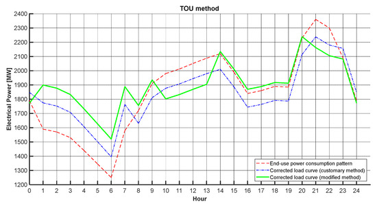
Figure 10.
Comparison of customary and modified TOU methods.
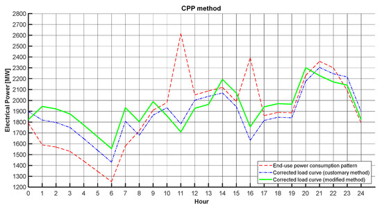
Figure 11.
Comparison of customary and modified CPP methods.
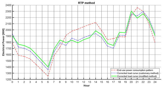
Figure 12.
Comparison of customary and modified RTP methods.
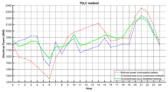
Figure 13.
Comparison of customary and modified TDLC methods.
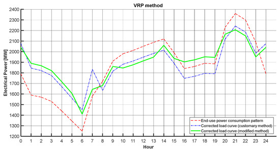
Figure 14.
Comparison of customary and modified VRP methods.
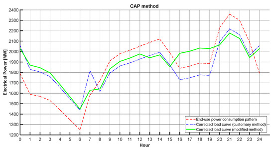
Figure 15.
Comparison of customary and modified CAP methods.
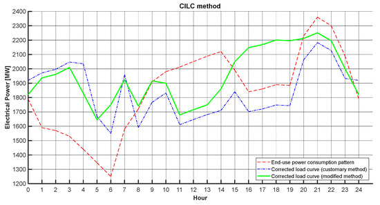
Figure 16.
Comparison of customary and modified CILC methods.
The results for the load factors were presented in Table 6. The results demonstrate the improvement of the situation for the modified model.
Table 6.
Load factors for simulation of modified DR comprehensive model.
6. Conclusions
This paper focused on the role and importance of productivity in the DSM arena. Foremost, a comprehensive discussion for indices of DSM was accomplished. Meanwhile, an inclusive DSM index was introduced that includes twofold productivity for energy and investment to analyze the productivity in the electrical energy systems. Afterward, a general classification of DSM was presented, and the pertaining modalities were clarified while considering the constituents of the mentioned DSM index. Since DR schemes are the most significant modalities of electrical load management in the smart grids, a DR model was developed that can ensure the implementation of three price-based and four incentive-based DR strategies in the smart microgrids. Moreover, the renovated payment principles were formulated to involve the flexibility of load drop and proliferation simultaneously. The contributions of this paper can be enumerated as follows:
- Reconsideration of DSM contexts from the productivity perspective,
- Innovation of a general DSM index containing the elementary attributes of energy management in the electrical energy systems,
- Developing a modified DR model that enhances the efficacious of load profile improvement in contrast with the conventional model,
- Embedment of rational payment criteria in the modified DR model that precisely determines the incentive and penalties by considering the unforeseeable reaction of the customers in energy consumption.
The simulation results of the DR proposed model show that the load factor can increase between 2.66% and 8.12% than the ordinary load curve. This demonstrates the accuracy and the merit of the modified model compared to the customary DR model because the load factor can be enhanced between 0.71% and 4.22% more than that of the customary DR model.
Author Contributions
Conceptualization, N.R. and M.D.; methodology, N.R. and M.D.; software, M.D.; validation, A.A.; formal analysis, M.D.; investigation, A.A.; resources, A.A.; data curation, A.A.; writing—original draft preparation, M.D.; writing—review and editing, M.D.; visualization, M.D.; supervision, N.R.; project administration, A.A.; All authors have read and agreed to the published version of the manuscript.
Funding
This research received no external funding.
Data Availability Statement
Not applicable.
Conflicts of Interest
The authors declare no conflict of interest.
Nomenclature
| Payment for change (PFC) rate at time t | |
| Initial load demand value at t-th hour | |
| Load demand value at t-th hour | |
| Load demand change at t-th hour | |
| Demand factor | |
| Demand-side management (DSM) index | |
| Contracted load demand | |
| Self-elasticity | |
| Cross-elasticity | |
| Delivered energy | |
| Demanded energy | |
| Available energy resource capacity | |
| Energy productivity | |
| Supplied energy | |
| Useful energy | |
| Capacity factor | |
| Delivery factor | |
| Utilization factor | |
| Distinction factor of hour types | |
| Unit ramp function | |
| Heaviside step function | |
| Dirac delta function | |
| Unit doublet function | |
| Consumption efficiency | |
| Grid efficiency | |
| Unified function of payment for change at t-th hour | |
| Peak load demand after load curve reshaping | |
| Peak load demand before load curve reshaping | |
| Function that describes suppliable electrical load curve | |
| System productivity | |
| Unified function of payment for deviation at t-th hour | |
| Unified function of total payment at t-th hour | |
| Payment for change (PFC) coefficient at t-th hour | |
| Payment for deviation (PFD) coefficient at t-th hour | |
| Adequacy coefficient | |
| Up-front reservation rate at t-th hour | |
| Load factor | |
| Load factor after load curve reshaping | |
| Load factor before load curve reshaping | |
| Amount of change in load factor | |
| Maximum suppliable electrical power | |
| Function that describes supplied electrical power curve | |
| Length of permissive band | |
| Regulation factor | |
| Initial electricity price at t-th hour | |
| Spot electricity price at t-th hour | |
| Electricity price change at t-th hour | |
| Payment for deviation (PFD) rate at t-th hour | |
| Final payment | |
| Payment for change at t-th hour | |
| Payment for deviation at t-th hour | |
| Function that describes load curve | |
| Fixed clipped load demand value | |
| Function that describes load curve after load curve reshaping | |
| Function that describes load curve before load curve reshaping | |
| Peak load demand | |
| Initial time | |
| Final time | |
| Total payment at t-th hour | |
| Boundary particular value of triplet bands |
References
- Kanakadhurga, D.; Prabaharan, N. Demand side management in microgrid: A critical review of key issues and recent trends. Renew. Sustain. Energy Rev. 2022, 156, 111915. [Google Scholar] [CrossRef]
- Chen, Y.; Xu, P.; Gu, J.; Schmidt, F.; Li, W. Measures to improve energy demand flexibility in buildings for demand response (DR): A review. Energy Build. 2018, 177, 125–139. [Google Scholar] [CrossRef]
- Afzalan, M.; Jazizadeh, F. Residential loads flexibility potential for demand response using energy consumption patterns and user segments. Appl. Energy 2019, 254, 113693. [Google Scholar] [CrossRef]
- Sharifi, R.; Fathi, S.; Vahidinasab, V. A review on Demand-side tools in electricity market. Renew. Sustain. Energy Rev. 2017, 72, 565–572. [Google Scholar] [CrossRef]
- Gelazanskas, L.; Gamage, K.A. Demand side management in smart grid: A review and proposals for future direction. Sustain. Cities Soc. 2014, 11, 22–30. [Google Scholar] [CrossRef]
- Scarabaggio, P.; Grammatico, S.; Carli, R.; Dotoli, M. Distributed Demand Side Management with Stochastic Wind Power Forecasting. IEEE Trans. Control Syst. Technol. 2022, 2, 97–112. [Google Scholar] [CrossRef]
- Strbac, G. Demand side management: Benefits and challenges. Energy Policy 2008, 36, 4419–4426. [Google Scholar] [CrossRef]
- Li, P.-H.; Pye, S. Assessing the benefits of demand-side flexibility in residential and transport sectors from an integrated energy systems perspective. Appl. Energy 2018, 228, 965–979. [Google Scholar] [CrossRef]
- Curiel, J.A.R.; Thakur, J. A novel approach for direct load control of residential air conditioners for demand side management in developing regions. Energy 2022, 258, 124763. [Google Scholar] [CrossRef]
- Yun, L.; Xiao, M.; Li, L. Vehicle-to-manufacturing (V2M) system: A novel approach to improve energy demand flexibility for demand response towards sustainable manufacturing. Appl. Energy 2022, 323, 119552. [Google Scholar] [CrossRef]
- Rosso, A.; Ma, J.; Kirschen, D.S.; Ochoa, L.F. Assessing the contribution of demand side management to power system flexibility. In Proceedings of the 2011 50th IEEE Conference on Decision and Control and European Control Conference, Orlando, FL, USA, 12–15 December 2011; pp. 4361–4365. [Google Scholar] [CrossRef]
- McPherson, M.; Stoll, B. Demand response for variable renewable energy integration: A proposed approach and its impacts. Energy 2020, 197, 117205. [Google Scholar] [CrossRef]
- Rana, J.; Rahi, K.H.; Ray, T.; Sarker, R. An efficient optimization approach for flexibility provisioning in community microgrids with an incentive-based demand response scheme. Sustain. Cities Soc. 2021, 74, 103218. [Google Scholar] [CrossRef]
- Chen, J.; Qi, B.; Rong, Z.; Peng, K.; Zhao, Y.; Zhang, X. Multi-energy coordinated microgrid scheduling with integrated demand response for flexibility improvement. Energy 2021, 217, 119387. [Google Scholar] [CrossRef]
- Wang, Y.; Huang, Y.; Wang, Y.; Zeng, M.; Li, F.; Wang, Y.; Zhang, Y. Energy management of smart micro-grid with response loads and distributed generation considering demand response. J. Clean. Prod. 2018, 197, 1069–1083. [Google Scholar] [CrossRef]
- Hajiamoosha, P.; Rastgou, A.; Bahramara, S.; Sadati, S.M.B. Stochastic energy management in a renewable energy-based microgrid considering demand response program. Int. J. Electr. Power Energy Syst. 2021, 129, 106791. [Google Scholar] [CrossRef]
- Dehghani, H.; Vahidi, B. Evaluating the effects of demand response programs on distribution cables life expectancy. Electr. Power Syst. Res. 2022, 213, 108710. [Google Scholar] [CrossRef]
- Aghaei, J.; Alizadeh, M. Critical peak pricing with load control demand response program in unit commitment problem. IET Gener. Transm. Distrib. 2013, 7, 681–690. Available online: http://digital-library.theiet.org/content/journals/10.1049/iet-gtd.2012.0739 (accessed on 29 August 2022). [CrossRef]
- Dogan, A.; Kuzlu, M.; Pipattanasomporn, M.; Rahman, S.; Yalcinoz, T. Impact of EV charging strategies on peak demand reduction and load factor improvement. In Proceedings of the 2015 9th International Conference on Electrical and Electronics Engineering (ELECO), Bursa, Turkey, 26–28 November 2015; pp. 374–378. [Google Scholar] [CrossRef]
- Chen, Y.; Xu, Z.; Wang, J.; Lund, P.D.; Han, Y.; Cheng, T. Multi-objective optimization of an integrated energy system against energy, supply-demand matching and exergo-environmental cost over the whole life-cycle. Energy Convers. Manag. 2022, 254, 115203. [Google Scholar] [CrossRef]
- Papagiannis, G.; Dagoumas, A.; Lettas, N.; Dokopoulos, P. Economic and environmental impacts from the implementation of an intelligent demand side management system at the European level. Energy Policy 2008, 36, 163–180. [Google Scholar] [CrossRef]
- Milovanoff, A.; Dandres, T.; Gaudreault, C.; Cheriet, M.; Samson, R. Real-time environmental assessment of electricity use: A tool for sustainable demand-side management programs. Int. J. Life Cycle Assess. 2018, 23, 1981–1994. [Google Scholar] [CrossRef]
- Baumgärtner, N.; Delorme, R.; Hennen, M.; Bardow, A. Design of low-carbon utility systems: Exploiting time-dependent grid emissions for climate-friendly demand-side management. Appl. Energy 2019, 247, 755–765. [Google Scholar] [CrossRef]
- Almohaimeed, S.A.; Suryanarayanan, S.; O’Neill, P. Reducing carbon dioxide emissions from electricity sector using demand side management. Energy Sources Part A Recover. Util. Environ. Eff. 2021, 1–21. [Google Scholar] [CrossRef]
- Rezaei, N.; Khazali, A.; Mazidi, M.; Ahmadi, A. Economic energy and reserve management of renewable-based microgrids in the presence of electric vehicle aggregators: A robust optimization approach. Energy 2020, 201, 117629. [Google Scholar] [CrossRef]
- Al Hadi, A.; Silva, C.A.S.; Hossain, E.; Challoo, R. Algorithm for Demand Response to Maximize the Penetration of Renewable Energy. IEEE Access 2020, 8, 55279–55288. [Google Scholar] [CrossRef]
- Harsh, P.; Das, D. Energy management in microgrid using incentive-based demand response and reconfigured network considering uncertainties in renewable energy sources. Sustain. Energy Technol. Assess. 2021, 46, 101225. [Google Scholar] [CrossRef]
- Zheng, S.; Sun, Y.; Li, B.; Qi, B.; Zhang, X.; Li, F. Incentive-based integrated demand response for multiple energy carriers under complex uncertainties and double coupling effects. Appl. Energy 2021, 283, 116254. [Google Scholar] [CrossRef]
- Ullah, S.; Khan, L.; Badar, R.; Ullah, A.; Karam, F.W.; Khan, Z.A.; Rehman, A.U. Consensus based SoC trajectory tracking control design for economic-dispatched distributed battery energy storage system. PLoS ONE 2020, 15, e0232638. [Google Scholar] [CrossRef] [PubMed]
- Mulleriyawage, U.; Shen, W. Impact of demand side management on optimal sizing of residential battery energy storage system. Renew. Energy 2021, 172, 1250–1266. [Google Scholar] [CrossRef]
- Huang, D.; Billinton, R. Effects of Load Sector Demand Side Management Applications in Generating Capacity Adequacy Assessment. IEEE Trans. Power Syst. 2012, 27, 335–343. [Google Scholar] [CrossRef]
- Zhu, L.; Yan, Z.; Lee, W.-J.; Yang, X.; Fu, Y.; Cao, W. Direct Load Control in Microgrids to Enhance the Performance of Integrated Resources Planning. IEEE Trans. Ind. Appl. 2015, 51, 3553–3560. [Google Scholar] [CrossRef]
- Mansouri, S.; Ahmarinejad, A.; Sheidaei, F.; Javadi, M.; Jordehi, A.R.; Nezhad, A.E.; Catalão, J. A multi-stage joint planning and operation model for energy hubs considering integrated demand response programs. Int. J. Electr. Power Energy Syst. 2022, 140, 108103. [Google Scholar] [CrossRef]
- Rezaei, N.; Tarimoradi, H.; Deihimi, M. A coordinated management scheme for power quality and load consumption improvement in smart grids based on sustainable energy exchange based model. Sustain. Energy Technol. Assess. 2022, 51, 101903. [Google Scholar] [CrossRef]
- Bruninx, K.; Pandžić, H.; Le Cadre, H.; Delarue, E. On the Interaction Between Aggregators, Electricity Markets and Residential Demand Response Providers. IEEE Trans. Power Syst. 2020, 35, 840–853. [Google Scholar] [CrossRef]
- Mohseni, S.; Brent, A.C.; Kelly, S.; Browne, W.N.; Burmester, D. Modelling utility-aggregator-customer interactions in interruptible load programmes using non-cooperative game theory. Int. J. Electr. Power Energy Syst. 2021, 133, 107183. [Google Scholar] [CrossRef]
- Rezaei, N.; Meyabadi, A.F.; Deihimi, M. A game theory based demand-side management in a smart microgrid considering price-responsive loads via a twofold sustainable energy justice portfolio. Sustain. Energy Technol. Assess. 2022, 52, 102273. [Google Scholar] [CrossRef]
- Lu, R.; Hong, S.H.; Zhang, X. A Dynamic pricing demand response algorithm for smart grid: Reinforcement learning approach. Appl. Energy 2018, 220, 220–230. [Google Scholar] [CrossRef]
- Tang, R.; Wang, S.; Li, H. Game theory based interactive demand side management responding to dynamic pricing in price-based demand response of smart grids. Appl. Energy 2019, 250, 118–130. [Google Scholar] [CrossRef]
- Affonso, C.; Da Silva, L.C.P.; Freitas, W. Demand-Side Management to Improve Power System Security. In Proceedings of the 2005/2006 IEEE/PES Transmission and Distribution Conference and Exhibition, Dallas, TX, USA, 21–24 May 2006; pp. 517–522. [Google Scholar] [CrossRef]
- Affonso, C.M.; da Silva, L.C. Potential benefits of implementing load management to improve power system security. Int. J. Electr. Power Energy Syst. 2010, 32, 704–710. [Google Scholar] [CrossRef]
- Wang, Y.; Pordanjani, I.R.; Xu, W. An Event-Driven Demand Response Scheme for Power System Security Enhancement. IEEE Trans. Smart Grid 2011, 2, 23–29. [Google Scholar] [CrossRef]
- Göransson, L.; Goop, J.; Unger, T.; Odenberger, M.; Johnsson, F. Linkages between demand-side management and congestion in the European electricity transmission system. Energy 2014, 69, 860–872. [Google Scholar] [CrossRef]
- Leithon, J.; Lim, T.J.; Sun, S. Battery-Aided Demand Response Strategy Under Continuous-Time Block Pricing. IEEE Trans. Signal Process. 2016, 64, 395–405. [Google Scholar] [CrossRef]
- Khan, I. Energy-saving behaviour as a demand-side management strategy in the developing world: The case of Bangladesh. Int. J. Energy Environ. Eng. 2019, 10, 493–510. [Google Scholar] [CrossRef]
- Ma, Z.; Zheng, Y.; Mu, C.; Ding, T.; Zang, H. Optimal trading strategy for integrated energy company based on integrated demand response considering load classifications. Int. J. Electr. Power Energy Syst. 2021, 128, 106673. [Google Scholar] [CrossRef]
- Parrish, B.; Heptonstall, P.; Gross, R.; Sovacool, B.K. A systematic review of motivations, enablers and barriers for consumer engagement with residential demand response. Energy Policy 2020, 138, 111221. [Google Scholar] [CrossRef]
- Harper, M. Review of Strategies and Technologies for Demand-Side Management on Isolated Mini-Grids; eScholarship; University of California: Los Angeles, CA, USA, 2013. [Google Scholar] [CrossRef]
- Oskouei, M.Z.; Şeker, A.A.; Tunçel, S.; Demirbaş, E.; Gözel, T.; Hocaoğlu, M.H.; Abapour, M.; Mohammadi-Ivatloo, B. A Critical Review on the Impacts of Energy Storage Systems and Demand-Side Management Strategies in the Economic Operation of Renewable-Based Distribution Network. Sustainability 2022, 14, 2110. [Google Scholar] [CrossRef]
- Jordehi, A.R. Optimisation of demand response in electric power systems, a review. Renew. Sustain. Energy Rev. 2019, 103, 308–319. [Google Scholar] [CrossRef]
- Nawaz, A.; Zhou, M.; Wu, J.; Long, C. A comprehensive review on energy management, demand response, and coordination schemes utilization in multi-microgrids network. Appl. Energy 2022, 323, 119596. [Google Scholar] [CrossRef]
- Yan, X.; Ozturk, Y.; Hu, Z.; Song, Y. A review on price-driven residential demand response. Renew. Sustain. Energy Rev. 2018, 96, 411–419. [Google Scholar] [CrossRef]
- Farsangi, A.S.; Hadayeghparast, S.; Mehdinejad, M.; Shayanfar, H. A novel stochastic energy management of a microgrid with various types of distributed energy resources in presence of demand response programs. Energy 2018, 160, 257–274. [Google Scholar] [CrossRef]
- Aussel, D.; Brotcorne, L.; Lepaul, S.; von Niederhäusern, L. A trilevel model for best response in energy demand-side management. Eur. J. Oper. Res. 2020, 281, 299–315. [Google Scholar] [CrossRef]
- Noor, S.; Yang, W.; Guo, M.; van Dam, K.H.; Wang, X. Energy Demand Side Management within micro-grid networks enhanced by blockchain. Appl. Energy 2018, 228, 1385–1398. [Google Scholar] [CrossRef]
- Gjorgievski, V.Z.; Markovska, N.; Abazi, A.; Duić, N. The potential of power-to-heat demand response to improve the flexibility of the energy system: An empirical review. Renew. Sustain. Energy Rev. 2020, 138, 110489. [Google Scholar] [CrossRef]
- Li, Y.; Wang, C.; Li, G.; Chen, C. Optimal scheduling of integrated demand response-enabled integrated energy systems with uncertain renewable generations: A Stackelberg game approach. Energy Convers. Manag. 2021, 235, 113996. [Google Scholar] [CrossRef]
- Li, Y.; Li, K.; Yang, Z.; Yu, Y.; Xu, R.; Yang, M. Stochastic optimal scheduling of demand response-enabled microgrids with renewable generations: An analytical-heuristic approach. J. Clean. Prod. 2022, 330, 129840. [Google Scholar] [CrossRef]
- Khalili, T.; Nojavan, S.; Zare, K. Optimal performance of microgrid in the presence of demand response exchange: A stochastic multi-objective model. Comput. Electr. Eng. 2019, 74, 429–450. [Google Scholar] [CrossRef]
- Yang, X.; Zhang, Y.; He, H.; Ren, S.; Weng, G. Real-Time Demand Side Management for a Microgrid Considering Uncertainties. IEEE Trans. Smart Grid 2019, 10, 3401–3414. [Google Scholar] [CrossRef]
- MansourLakouraj, M.; Shahabi, M.; Shafie-Khah, M.; Catalão, J.P. Optimal market-based operation of microgrid with the integration of wind turbines, energy storage system and demand response resources. Energy 2022, 239, 122156. [Google Scholar] [CrossRef]
- Kumar, R.S.; Raghav, L.P.; Raju, D.K.; Singh, A.R. Impact of multiple demand side management programs on the optimal operation of grid-connected microgrids. Appl. Energy 2021, 301, 117466. [Google Scholar] [CrossRef]
- Groppi, D.; Pfeifer, A.; Garcia, D.A.; Krajačić, G.; Duić, N. A review on energy storage and demand side management solutions in smart energy islands. Renew. Sustain. Energy Rev. 2020, 135, 110183. [Google Scholar] [CrossRef]
- Golmohamadi, H. Demand-side management in industrial sector: A review of heavy industries. Renew. Sustain. Energy Rev. 2021, 156, 111963. [Google Scholar] [CrossRef]
- Warren, P. A review of demand-side management policy in the UK. Renew. Sustain. Energy Rev. 2014, 29, 941–951. [Google Scholar] [CrossRef]
- Meyabadi, A.F.; Deihimi, M. A review of demand-side management: Reconsidering theoretical framework. Renew. Sustain. Energy Rev. 2017, 80, 367–379. [Google Scholar] [CrossRef]
- Jabir, H.J.; Teh, J.; Ishak, D.; Abunima, H. Impacts of Demand-Side Management on Electrical Power Systems: A Review. Energies 2018, 11, 1050. [Google Scholar] [CrossRef]
- Dranka, G.G.; Ferreira, P. Review and assessment of the different categories of demand response potentials. Energy 2019, 179, 280–294. [Google Scholar] [CrossRef]
- Mariano-Hernández, D.; Hernández-Callejo, L.; Zorita-Lamadrid, A.; Duque-Pérez, O.; García, F.S. A review of strategies for building energy management system: Model predictive control, demand side management, optimization, and fault detect & diagnosis. J. Build. Eng. 2021, 33, 101692. [Google Scholar] [CrossRef]
- Kara, D. Implementing Productivity Based Demand Response in Office Buildings Using Building Automation Standards. Ph.D. Thesis, Durham University, Durham, UK, 2015. [Google Scholar]
- Dorahaki, S.; Abdollahi, A.; Rashidinejad, M.; Moghbeli, M. The role of energy storage and demand response as energy democracy policies in the energy productivity of hybrid hub system considering social inconvenience cost. J. Energy Storage 2021, 33, 102022. [Google Scholar] [CrossRef]
- Sarker, E.; Seyedmahmoudian, M.; Jamei, E.; Horan, B.; Stojcevski, A. Optimal management of home loads with renewable energy integration and demand response strategy. Energy 2020, 210, 118602. [Google Scholar] [CrossRef]
- Gangwar, S.; Bhanja, D.; Biswas, A. Cost, reliability, and sensitivity of a stand-alone hybrid renewable energy system—A case study on a lecture building with low load factor. J. Renew. Sustain. Energy 2015, 7, 013109. [Google Scholar] [CrossRef]
- Chiu, W.-Y.; Hsieh, J.-T.; Chen, C.-M. Pareto Optimal Demand Response Based on Energy Costs and Load Factor in Smart Grid. IEEE Trans. Ind. Inform. 2020, 16, 1811–1822. [Google Scholar] [CrossRef]
- Bobby, S.R. Chapter 6 Demand, Load Factor, Service Factor, and Electrical Power Bill Computation. In Electrical Engineering for Non-Electrical Engineers©; River Publishers: Roma, Italy, 2021; pp. 195–208. [Google Scholar]
- Gotham, D.; Muthuraman, K.; Preckel, P.; Rardin, R.; Ruangpattana, S. A load factor based mean–variance analysis for fuel diversification. Energy Econ. 2009, 31, 249–256. [Google Scholar] [CrossRef]
- Bhattacharya, M.; Inekwe, J.N.; Sadorsky, P.; Saha, A. Convergence of energy productivity across Indian states and territories. Energy Econ. 2018, 74, 427–440. [Google Scholar] [CrossRef]
- Huo, T.; Ren, H.; Cai, W.; Feng, W.; Tang, M.; Zhou, N. The total-factor energy productivity growth of China’s construction industry: Evidence from the regional level. Nat. Hazards 2018, 92, 1593–1616. [Google Scholar] [CrossRef]
- Bhattacharya, M.; Inekwe, J.N.; Sadorsky, P. Convergence of energy productivity in Australian states and territories: Determinants and forecasts. Energy Econ. 2019, 85, 104538. [Google Scholar] [CrossRef]
- Dinu, M.; Pătărlăgeanu, S.R.; Petrariu, R.; Constantin, M.; Potcovaru, A.-M. Empowering Sustainable Consumer Behavior in the EU by Consolidating the Roles of Waste Recycling and Energy Productivity. Sustainability 2020, 12, 9794. [Google Scholar] [CrossRef]
- Doojav, G.-O.; Kalirajan, K. Sources of energy productivity change in Australian sub-industries. Econ. Anal. Policy 2020, 65, 1–10. [Google Scholar] [CrossRef]
- Lin, B.; Sai, R. Sustainable transitioning in Africa: A historical evaluation of energy productivity changes and determinants. Energy 2022, 250, 123833. [Google Scholar] [CrossRef]
- Krarti, M.; Dubey, K.; Howarth, N. Energy productivity analysis framework for buildings: A case study of GCC region. Energy 2019, 167, 1251–1265. [Google Scholar] [CrossRef]
- Chang, R.; Lu, C. Feeder reconfiguration for load factor improvement. In Proceedings of the 2002 IEEE Power Engineering Society Winter Meeting, Conference Proceedings (Cat. No.02CH37309). New York, NY, USA, 27–31 January 2002; Volume 2, pp. 980–984. [Google Scholar] [CrossRef]
- Cerna, F.V.; Pourakbari-Kasmaei, M.; Naderi, E.; Lehtonen, M.; Contreras, J. Load Factor Assessment of the Electric Grid by the Optimal Scheduling of Electrical Equipment- A MIQCP Model. IEEE Open Access J. Power Energy 2021, 8, 433–447. [Google Scholar] [CrossRef]
- Kubule, A.; Ločmelis, K.; Blumberga, D. Analysis of the results of national energy audit program in Latvia. Energy 2020, 202, 117679. [Google Scholar] [CrossRef]
- Rodriguez, A.; Smith, S.T.; Potter, B. Sensitivity analysis for building energy audit calculation methods: Handling the uncertainties in small power load estimation. Energy 2022, 238, 121511. [Google Scholar] [CrossRef]
- Zhang, J.; Liu, W.; Tian, Z.; Qi, H.; Zeng, J.; Yang, Y. Urban Rail Substation Parameter Optimization by Energy Audit and Modified Salp Swarm Algorithm. IEEE Trans. Power Deliv. 2022. [Google Scholar] [CrossRef]
- Raza, M.Y.; Lin, B. Energy efficiency and factor productivity in Pakistan: Policy perspectives. Energy 2022, 247, 123461. [Google Scholar] [CrossRef]
- Loughran, D.S.; Kulick, J. Demand-Side Management and Energy Efficiency in the United States. Energy J. 2004, 25, 19–44. [Google Scholar] [CrossRef]
- Andersson, E.; Karlsson, M.; Thollander, P.; Paramonova, S. Energy end-use and efficiency potentials among Swedish industrial small and medium-sized enterprises—A dataset analysis from the national energy audit program. Renew. Sustain. Energy Rev. 2018, 93, 165–177. [Google Scholar] [CrossRef]
- Locmelis, K.; Blumberga, D.; Blumberga, A.; Kubule, A. Benchmarking of Industrial Energy Efficiency. Outcomes of an Energy Audit Policy Program. Energies 2020, 13, 2210. [Google Scholar] [CrossRef]
- Klemm, C.; Wiese, F. Indicators for the optimization of sustainable urban energy systems based on energy system modeling. Energy Sustain. Soc. 2022, 12, 1–20. [Google Scholar] [CrossRef]
- Aalami, H.; Moghaddam, M.P.; Yousefi, G. Demand response modeling considering Interruptible/Curtailable loads and capacity market programs. Appl. Energy 2010, 87, 243–250. [Google Scholar] [CrossRef]
- Aalami, H.; Moghaddam, M.P.; Yousefi, G. Modeling and prioritizing demand response programs in power markets. Electr. Power Syst. Res. 2010, 80, 426–435. [Google Scholar] [CrossRef]
- Yousefi, S.; Moghaddam, M.P.; Majd, V.J. Optimal real time pricing in an agent-based retail market using a comprehensive demand response model. Energy 2011, 36, 5716–5727. [Google Scholar] [CrossRef]
- Baboli, P.T.; Eghbal, M.; Moghaddam, M.P.; Aalami, H. Customer behavior based demand response model. In Proceedings of the 2012 IEEE Power and Energy Society General Meeting, San Diego, CA, USA, 22–26 July 2012; pp. 1–7. [Google Scholar] [CrossRef]
- Aalami, H.; Moghaddam, M.P.; Yousefi, G. Evaluation of nonlinear models for time-based rates demand response programs. Int. J. Electr. Power Energy Syst. 2015, 65, 282–290. [Google Scholar] [CrossRef]
- Astriani, Y.; Shafiullah, G.; Shahnia, F. Incentive determination of a demand response program for microgrids. Appl. Energy 2021, 292, 116624. [Google Scholar] [CrossRef]
- Aïd, R.; Possamaï, D.; Touzi, N. Optimal Electricity Demand Response Contracting with Responsiveness Incentives. Math. Oper. Res. 2022, 1–36. [Google Scholar] [CrossRef]
- Lynch, M.; Nolan, S.; Devine, M.T.; O’Malley, M. The impacts of demand response participation in capacity markets. Appl. Energy 2019, 250, 444–451. [Google Scholar] [CrossRef]
- Wang, B.; Li, Y.; Ming, W.; Wang, S. Deep Reinforcement Learning Method for Demand Response Management of Interruptible Load. IEEE Trans. Smart Grid 2020, 11, 3146–3155. [Google Scholar] [CrossRef]
- Azuatalam, D.; Lee, W.-L.; de Nijs, F.; Liebman, A. Reinforcement learning for whole-building HVAC control and demand response. Energy AI 2020, 2, 100020. [Google Scholar] [CrossRef]
- Irtija, N.; Sangoleye, F.; Tsiropoulou, E.E. Contract-Theoretic Demand Response Management in Smart Grid Systems. IEEE Access 2020, 8, 184976–184987. [Google Scholar] [CrossRef]


Publisher’s Note: MDPI stays neutral with regard to jurisdictional claims in published maps and institutional affiliations. |
© 2022 by the authors. Licensee MDPI, Basel, Switzerland. This article is an open access article distributed under the terms and conditions of the Creative Commons Attribution (CC BY) license (https://creativecommons.org/licenses/by/4.0/).