Abstract
The attention paid to energy consumption is growing steadily due to the costs associated with energy usage as well as the resulting environmental impacts. This work proposes an analytical method to assess the energy consumption and the power requirements of a productive system. By exploiting queuing theory, it is possible to achieve a probabilistic view of energy consumption. This method is useful to define the contractual power level and calculate the service level associated with it, so it is applicable as a decision-support tool during the design of productive systems when it is not possible to obtain field data (green-field design). Three different models characterised by an increasing degree of complexity were exploited. The three models share the feature of an infinite number of servers, while the increasing complexity is due to the introduction of batch arrivals and the variability of the size of the arrival lot. A connection is made between production variables and power used by machines to consider energy consumption. A numerical example shows the applicability of the method and highlights the different results obtained through the three models. In addition, analytical formulations are available for all three proposed models; thus, no simulation process is needed.
1. Introduction
In manufacturing systems, managers usually study processes according to concepts and performance indicators such as throughput, WIP (work in process), inventory level and service level. These indicators are useful instruments in order to carry out AS-IS analyses (i.e., study of the current state of a system) and estimate the impact of variations in the production variables. The relevance of the evaluation of these aspects is well known; in fact, it is possible to find several models and methodologies that propose to optimise production processes exploiting this set of indicators. By dealing with productive performances, the evaluation of energy consumption has become a crucial factor in the study of production processes. Thus, the reduction in energy-related costs has become a strategic lever for competitiveness and improvement of business performance [1,2]. This is due, on the one hand, to the classical cost reduction and, on the other hand, to the growing attention to environmental sustainability. This study deals with energy consumption in a manufacturing system and, more specifically, the evaluation of the contractual power level, which corresponds to a significant cost item within the energy supply contract. Moreover, contracts with suppliers foresee a maximum power level, which, if exceeded, causes significant penalties from an economic point of view. Therefore, it is important to evaluate the service level offered by a given contractual power level by considering the variability of the production activities and of the related power. Specifically, ref. [3] defines the service level associated with a given power level as the probability of a power request being lower than the power contractual level. In addition, the importance of careful evaluation of the contractual power level is corroborated by the increase in energy-related costs that have occurred over the past few years. In particular, a connection will be made between classical production variables, such as the activation rate of machines, the duration of the processing and energy consumption. As stated before, each of the variables mentioned is characterised by variability, which is reflected in substantial variations in energy consumption and, consequently, in power required for the system operation. As a result, energy consumption is difficult to predict. In particular, in this work, we studied the definition of the power level in the design phase of productive systems. During this phase, it is possible to know only some information about the product and machines (i.e., estimated demand and estimation of the production phases and machines and related cycle time). Therefore, the method proposed in this study takes into account the information that it is possible to have or estimate during the design phase and, at the same time, attempts to model the variability of processes and consumption through the use of stochastic techniques in order to intercept a greater realism in the representation and analysis of the system under consideration. Therefore, the potentialities of the models of queuing theory were exploited in order to have a dynamic and stochastic vision of the power requirements of the system.
The traditional method for the calculation of the contractual power level in the design phase is based on the load factor and the coincidence factor. The first factor relates to the individual device and is defined as the ratio of the machine’s mean load to its nominal power, while the second takes into account multiple users and their overlapping power demands, so it is calculated as the peak of a system divided by the sum of the peak loads of its individual components. The traditional method relies solely on load factor, and coincidence factor provides a static view of the system and its power requirements, while the method proposed in this study, exploiting queuing theory, provides a probabilistic view of consumption and power requirements allowing for more conscientious managerial assessment by exploiting the product and machine information available during the design phase of productive systems. Hence, this method can be applied as a design tool, for example, in green-field contexts or for the evaluation of investments such as expansions or production increases. Moreover, relying on elementary production data (such as the nominal power of machines, machining cycles, production times, etc.) that can be easily estimated and obtained allows a dynamic and probabilistic view of the energy requirements of the system under consideration. This paper seeks to provide an alternative tool for decision support. In particular, it presents a method, based on queuing theory, for the calculation of the contractual power level and the associated service level. The latter information (i.e., the service level) is useful to make economic assessments of the possibility of incurring contractual penalties caused by exceeding the maximum power level. Furthermore, it is important to emphasise that the proposed method is not intended as an operational management or monitoring tool for productive systems. Therefore, operational decisions dealing with power or energy consumption (e.g., machine on/off criterion, energy-aware scheduling, etc.) are not within the domain of this model [4,5,6]. Energy operational management and monitoring are aspects commonly analysed through the tools and methods offered by Industry 4.0. For example, the developments in sensor technology have enabled the timely and accurate measurement of energy consumption at the individual machine level, paving the way for more effective operational decisions. The scientific literature is replete with contributions describing new types of sensors and their applications; for example, in [7,8], the potentials of IoT-based sensors in terms of ease of data extraction and implementation are highlighted. The paper is organised as follows: in Section 2, the literature review is presented; Section 3 introduces the models and their formulation; Section 4 offers a numerical example along with numerical results and sensitivity analysis; and finally, Section 5 covers conclusions and suggestions for discussion.
2. Literature Review
The scientific literature is rich in contributions dealing with energy consumption in manufacturing, but the issue concerning the evaluation of the contractual power level through a stochastic model does not result in being in-depth. Ref. [3] proposed a queuing-theory-based method for the definition and evaluation of an adequate contractual power level. The methodology is based on a connection between production variables, such as machine activation rate, process duration and power consumption. As highlighted, the present contribution, starting from the paper of [3], proposes an improvement of the suggested method by adding degrees of complexity and realism to the methodology. In [9], a method based on a mathematical model for the calculation of energy consumption of machinery and plants was proposed. The work focuses on the single machine level, while the present paper proposes a method applicable to different contexts, e.g., a numerical application of a job-shop context is provided. Ref. [10] proposed a mathematical model for managerial decision support aimed at more efficient use of energy. Therefore, the model identifies a set of production sequences that minimise energy consumption and, at the same time, optimise completion time. In addition to the mathematical model, the paper provides numerous energy-aware dispatching rules. Since all the proposed methods are aimed at operational production management, they cannot be exploited for the definition of the contractual power level. In [11], a mathematical model was created to optimise and plan the energy savings for a given production schedule in order to define energy-aware scheduling (EAS). The proposed approach integrates an advanced planning and scheduling (APS) system that does not consider energy savings with a mixed integer programming (MIP) model in which the APS schedule is modified to evaluate energy consumption. The method does not consider variability in power requirements; moreover, the average power requirement is assumed to be known and constant during the job processing on the machines. Ref. [12] proposed a model based on queuing theory and queuing networks to evaluate the reduction in energy waste. Specifically, the individual machine is modelled as an M/M/1 model, while the production system is expressed as a network of M/M/1 queues. The model proves useful in the design stages to evaluate alternative production scenarios and assess potential energy savings. However, the model is not aimed at defining the contractual power level. In [13], a buffer-based method was proposed to achieve a reduction in energy consumption and subsequent costs while maintaining an adequate level of throughput. Therefore, a nonlinear programming (NIP) model with a constraint on the throughput level was developed. The model is useful for operational scheduling of processing and buffer management, so it is not a design tool for evaluating plant power levels. In [14], an analytical model for single-product production in two sequential stages was proposed. The model considers the different energy consumptions between the idle state, productive state and switch-off state; it also allows for variations in the production rate at each stage. The model is aimed at minimising production costs, paying attention to the cost items related to energy consumption, but as it requires a variety of complex operational data, it does not lend itself to use as a tool in the design phase. Ref. [15] proposed a method for defining intelligent scheduling that, in order to minimise energy consumption, merges small periods with longer periods of machine idle in order to achieve energy savings by avoiding on/off switch consumptions. In addition, the total weighted tardiness of jobs was also minimised. The environment considered is a job shop, and to solve the problem, the authors develop a multi-objective genetic algorithm. Therefore, the method is suitable for operational programming and not for the study of power requirements during the design phase. Ref. [16] developed a mathematically formulated scheduling that takes into account both energy efficiency and labour-related costs. In addition, a heuristic algorithm is proposed for the solution of the MILP problem. Ref. [17] proposed a scheduling model for asynchronous production line systems that aims for a good level of trade-off between energy consumption and production rate in demand–response contexts. As in the previous contribution, the focus was on the definition of an energy-efficient schedule and not on the evaluation of the power requirements of the system under consideration. Ref. [18] integrated energy assessments to the economic lot scheduling problem (ELSP). Idle, production and tool-change phases were considered in the model in order to minimise energy consumption, tool changes and holding costs. Therefore, the proposed method is useful for establishing a schedule that pays attention to energy aspects but does not suit the evaluation of the contractual power level. In [19], a job-shop scheduling problem with energy aspects was studied. The goal was to minimise the production costs in terms of energy, with the peculiarity of the presence of a power peak limitation, together with the traditional production constraints. The method does not consider variability in power consumption, in fact, each operation on a certain machine has a power consumption constant over its duration. The problem formulation was modelled using two alternative integer linear programming models. Ref. [20] studied a task-oriented modelling method in order to evaluate the energy consumption for a machining manufacturing system. A methodology of event graphs was exploited in order to model the consumption of energy driven by the tasks; subsequently, through simulation, flexible processes of tasks for optimising energy consumption were found. The tasks are obtained considering different constant and known power consumption values. Ref. [21] proposed a numerical model that seeks to align the power requirements of the production system with energy availability from renewable sources in order to maximize profits. The model considers numerous production and economic variables, so unlike the present contribution, it requires data that are not elementary and probably, hardly available. Ref. [22] developed a method, MILP model and solving algorithm for the definition of schedule that is integrated with the use of renewable energy. In particular, the article considers onsite renewable sources, energy storage systems and the classical power grid. The method does not consider stochastic distributions for energy availability and energy consumption. Ref. [23] developed a scheduling model capable of optimising energy consumption by exploiting three different strategies: machine off/on criterion, speed-scaling policy and transportation optimisation strategy. The problem was modelled through mixed integer linear programming, and the resolution was accomplished through an enhanced cooperative co-evolutionary algorithm (ECCA). As in other previously mentioned models, this fits the operating schedule definition and not the evaluation of the power level needed by the system. Ref. [24] developed an energy consumption cross-level model for a demand driven machine tool in a manufacturing environment. The model considers several states of the machines, in fact, it describes, through a Markovian general threshold model, the stochastic behaviours (failures, blocking, starvation) and inter-machine interactions. The model is suitable for the study of contexts characterised by two interacting machines. Ref. [25] proposed a prediction model for the energy consumption, completion time and probability of processing routes. The power consumption related to the different operations is known and constant. This model exploits the graphical evaluation and review technique (GERT) to describe the remanufacturing process. The present work proposes an alternative method for the definition and evaluation of the contractual power level during the design phase of production systems. In particular, the potential of queuing theory models was exploited. Operationally, a connection between system production variables and system energy consumption was considered, also evaluating stochastic distributions in order to take into account the variability of machine energy consumption. Specifically, three different queuing theory models were proposed, which present different degrees of complexity in order to achieve a greater realism in the representation of the energy consumption of the system.
3. Introduction to the Models
Every queuing model presented in this study shares a common feature: an infinite number of servers. This characteristic leads to a particular behaviour of the system; for each customer/job (kW of power under the assumption of this work) that reaches the system, there is always an available server. In other terms, no queue creation occurs. This specific behaviour is useful to represent the energy demand to the supply channel (Figure 1).
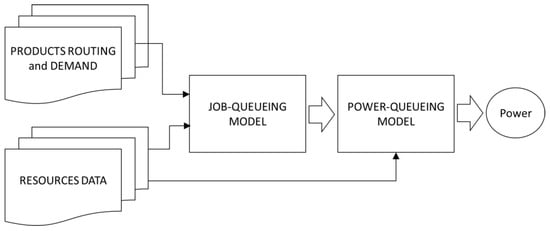
Figure 1.
Job-queueing and power-queueing models relationship [3].
The first analytical model that was analysed was an M/M/∞ according to Kendall–Lee notation. This model is the same one proposed in [3], where a job-queuing model and a power-queuing model are linked. The parameters are determined as follows:
where:
- , respectively, indicate the nominal power and the load factor of the i-th department;
- represents the arrival rate of power customers;
- indicates the arrival rate of jobs of the i-th department.
By considering the whole system, composed of N different departments, the following expressions hold:
where:
- represents the service rate considering the power queuing model and the whole system;
- represents the service rate of the i-th department.
In addition, it is possible to calculate the probability associated with the different states of the system in the steady state (i.e., in the queuing theory, the status in which the probabilities of the states of the system are independent of time). In particular, the states of the system correspond to kW of power under the assumptions made previously. The calculation for the probability of the state j takes the following form:
This expression allows evaluating the service level of a given power level, for instance, the contractual power level. In fact, the simple cumulative value of probability up to the desired kW level returns the service level associated.
The second model is characterised by the presence of an arrival lot (of constant size in first approximation); thus, it adds a degree of complexity. In particular, the higher complexity intercepts a higher realism in the system’s representation. Moreover, the simultaneity of arrivals, represented by an arrival lot, allows for maintaining the link between the queuing model and the frequency of activation of the machines (expressed by the arrival rate ), while considering the power as a multiplying factor of the arrival rate, this link loses its meaning. The difference mentioned above can be appreciated through the example of Figure 2. The substantial difference between unit arrivals and batch arrivals is highlighted, which is the simultaneity of N arrivals in the case of batch arrivals (N = 10 in the example of Figure 2) and N different single arrivals in the case of unit arrivals.
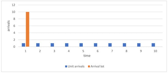
Figure 2.
Difference between unit arrivals and batch arrivals.
Using power as a multiplicative factor for the arrivals rate disaggregates the arrival batch into a series of arrivals of unit size.
According to Kendall–Lee notation, the presence of batch arrival determines an Mn/M/∞ queuing model. In summary, this additional feature improves the model proposed by [3] in terms of the ability to describe the system under analysis.
The presence of a batch arrival involves some adjustments for the determination of the usual queuing theory parameters. In particular, the power is no longer considered as a multiplying factor of the arrival rate but as the size of the arrival lot. Starting from the size of the arrival lot, N, it is set equal to:
where: , respectively, indicate the mean of the nominal powers of the departments and the mean of the load factors of the departments.
While the arrival rate and the service rate of the whole system, respectively, take the following formulations:
For the calculation of the probability of the states, the model Mx/M/c found in [26] was exploited. Since it was not possible to find a model with infinite servants and batch arrivals, the model previously mentioned was used. The latter is characterised by an arrival lot (constant or variable) and a finite number of servants (c), but by calculating the probability of the states using a number of servants sufficiently large to be considered infinite, the result approximates the case with an infinite number of servants. This procedure, i.e., the approximation of an infinite-servant model by considering a sufficiently large finite number of servants, can also be found in [27].
The formulas of this model [26] for the calculation of the probabilities of the states are in recursive form as follows:
where:
- is the number of servants;
- is the lot size in the constant case or the average lot size in the variable case;
- is the ratio between the arrival rate and the service rate;
- is the probability associated with the state ;
- is the probability that an arriving group has size .
Obviously, considering an arrival lot of constant size, the parameter would be activated (i.e., equal to 1) only when s is equal to .
The last model analysed in this study can be defined as an Mx/M/∞ following the Kendall–Lee notation. The letter x indicates the presence of an arrival lot of variable size. This feature of the model involves an additional degree of complexity. The variability of batch size is useful to describe the fluctuating energy consumption of the system, again in order to achieve greater realism. The Mx/M/c found in [26] results adequate to represent the wished context; the formulas are (8) and (9), and the parameters keep the meaning previously explained.
In addition, it is possible to study the behaviour of the system by calculating the performance parameter L. L commonly denotes the average number of customers in the system, but under the assumptions used to construct the models in this study, it indicates the average kW of power required by the system. The formula for the calculation of the L parameter for the M/M/∞ model is well-known in the literature and takes the following form:
For the Mn/M/∞ model, it was possible to find a formula for the calculation of L; the contribution was found in [28]. The formula is presented as follows:
where is equal to the lot size.
By analysing the previous Formula (11), it is clear that it gives the same result as the M/M/∞ one (10); as anticipated for the M/M/∞ model, the size of the arrival lot is considered as a multiplicative factor of the arrival rate. In other terms:
With regard to the Mx/M/∞ model, a direct formula for calculating the performance parameter L could not be found.
4. Numerical Application
In order to demonstrate the applicability of the models and to highlight the differences in the system’s representation, a numerical application was exploited. In particular, the same numerical example of [3] was proposed. Then the average product demand of the whole system is equal to 15 jobs/h, the average service time is equal to 0.05 h and the job shop is made of four different departments: D1, D2, D3 and D4. The jobs then have four different routings:
- 25% of jobs visiting department D1, then D3 and, finally, D4;
- 25% of jobs visiting department D1, then D2, D3 and, finally, D4;
- 25% of jobs visiting department D2, then D3 and, finally, D4;
- 25% of jobs visiting department D2 then D4.
Given that no changes have been made to the numerical values of the example and to the logic of operation of the first model, the displayed results of the job-queuing model and the M/M/∞ model report the same values as the article [3].
The first two tables, Table 1 and Table 2, show the parameters of the job-queuing model and the first model proposed (i.e., M/M/∞). The parameters of Table 2 are obtained considering and .

Table 1.
Arrival rate, service rate and utilisation rate of the departments.
Table 2.
Arrival rate and service rate of M/M/∞ model.
As mentioned before, the second model introduces the arrival lot (of size N), set equal to the multiplication between the nominal power and the load factor . Thus, the parameters of the Mn/M/∞ assume the values shown in Table 3.
Table 3.
Lot size, arrival rate and service rate of Mn/M/∞ model.
In order to better understand the meaning of the lot measurement unit (arrival/h), it can be seen as the number of machines activated per hour. Each of these activations involves energy consumption and then a power request.
Regarding the third model, it considers the variability in energy consumption. Therefore, the size of the arrival lot varies according to a certain probability distribution. In particular, a normal distribution of the mean (μ) equal to was chosen. By fixing the value of the coefficient of variation (CV), it is possible to obtain the value of the standard deviation (σ) of the normal distribution. Therefore, a value CV = 0.25 was selected, and as a result of the relation , the value was calculated. The CV value equal to 0.25 corresponds to low variability in batch size distribution. Table 4 reports the numerical values of the parameters.
Table 4.
Lot size distribution, arrival rate and service rate of Mx/M/∞ model.
4.1. Results
In this section, the results of the three different models are reported; in particular, the probability distributions of the steady states and the calculation, by the direct formula where possible, of the performance parameter L are presented. Figure 3 reports the probability distributions of the states obtained through the different models studied. Before commencing the results, it is necessary to underline that for the calculation of the probabilities of the states in the batch arrival case, 10,000 servants were considered (i.e., c = 10,000) in order to approximate the dynamics of a model with infinite servants.
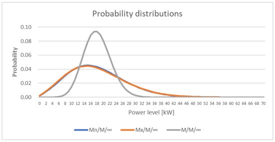
Figure 3.
Probability distributions of the states for the three models.
As it is possible to appreciate graphically, the models with lot arrivals (Mn/M/∞ and Mx/M/∞) have distributions of probability with a smoother shape. It is also interesting to note that with the CV value under consideration, the model with a constant size arrival lot and the one with a variable size provide almost identical values. In order to demonstrate what was previously stated, the value of mean absolute deviation was calculated between the two lot models, considering the first 45 states, from state 0 to state 44, an arbitrary choice due to the fact that this portion of the states contains more than 99% probability for both models, more precisely 99.05% for the variable lot size model and 99.45% for the constant lot size model. The result of this calculation gives a MAD (i.e., mean absolute deviation) value equal to 0.000582. The MAD value can be calculated as follows:
where:
- is the number of values that are considered;
- and , are the values of the two different sets that are considered.
Table 5 reports additional information about the model’s results. The information regarding the most probable state and the associated probability quantitatively expresses what was previously highlighted graphically. Moreover, the performance parameter L indicates the average kW required by the system under analysis.
Table 5.
Most probable state, probability of the most probable state and performance parameter L for the three models.
As mentioned above, it was not possible to find an analytical formula for the calculation of the parameter L for the Mx/M/∞ model. Therefore, L was calculated with the following formula that is valid for every queuing theory model:
In order to make it possible to calculate the parameter L for the Mx/M/∞ model using the previous formula, it was necessary to make an arbitrary choice; in particular, the calculation stopped at state 130. This value (130) was chosen because the calculation of L provides a value that tends to stabilise as shown in Figure 4. Even in terms of the L parameter, models with arrival batch variability and constant batch size present a difference of 0.008 kW.
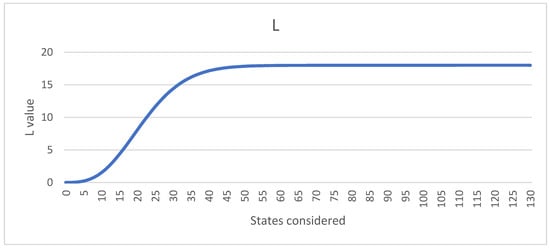
Figure 4.
Stabilisation in the calculation of parameter L.
As mentioned before, this application of queuing theory models allows evaluation of the power contractual level in terms of service level. It is intuitive that the service level varies depending on the model used due to the differences in the probability distributions of the states of the system that are appreciable in Figure 3. Following the reasoning proposed in [3], the standard method for calculating the contracted power level involves considering the load factor and coincidence factor. According to [29], it is standard that these factors share the same value of 0.8 in the system under consideration. Therefore, the calculation leads to a contractual power level of 25.6 kW.
Table 6 shows the different service levels and the power contractual level associated with the 99% service level according to the three different models. It is clear how the introduction of the arrival lot instead of the simpler case of unit arrivals gives a more pessimist result. The differences in service level calculations are related to the fact that the Mn/M/∞ and Mx/M/∞ models provide a flatter probability distribution of states than the M/M/∞ model, as can be observed in Figure 3. In particular, models associated with a higher degree of realism and complexity expect a larger probability of exceeding the contracted power level.
Table 6.
Comparison of the calculated service levels of the three models.
4.2. Sensitivity Analysis
Two different sensitivity analyses were carried out in order to evaluate the behaviour of the three different models.
The first analysis was conducted by applying percentage changes to the ratio between the arrival rate and the service rate (i.e., the system utilisation rate). These percentage changes were applied to all three proposed models. Specifically, the system utilisation rate underwent the following eight variations: +20%, +30%, …, +80%, +90%. These could represent, for example, an increase in machine activation frequency (i.e., the system arrival rate). The analysis highlighted how the behaviour presented by the three different models is also repeated after the variations mentioned above. For every percentage variation evaluated, the simplest model (M/M/∞) returns the highest service level values at the same power level; the Mx/M/∞ model, the most complex, returns the lowest service level values; and the Mn/M/∞ model calculates intermediate service level values with respect to the previous two. Figure 5 shows the power level required to achieve a 90% service level for the three different models in the evaluated scenarios.
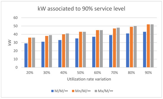
Figure 5.
kW value required for 90% service level by varying the utilisation rate of the three models.
Moreover, it can be observed that the M/M/∞ model always yields lower power levels to achieve a 90% service level. For the two models with arrival lot, the power level values are very close to the coefficient of variation considered (CV = 0.25). In addition, it is interesting to observe that the power level required to reach the 90% service level increases as the system utilisation rate increases. This behaviour is logical since by increasing the rate of arrivals (indirectly through the utilisation rate), which, as anticipated, represents the frequency of activation of the machines, with an equal duration of machining, there is an increase in energy consumption.
The second sensitivity analysis was performed to assess the impact of variability in arrival lot size. Specifically, alterations were made to the CV value, which directly impacts the magnitude of the standard deviation of the normal distribution governing lot size. Three different alternative CV values to the original 0.25 were evaluated: 0.5, 0.75 and 1. As can be observed in Figure 6, by increasing the variability of the distribution of the lot size (i.e., by increasing the CV), the probability distribution of the states of the system becomes increasingly flat. This behaviour, as also noted in the previous section, results in a higher probability of contracted power level overruns (i.e., a deterioration in service level).
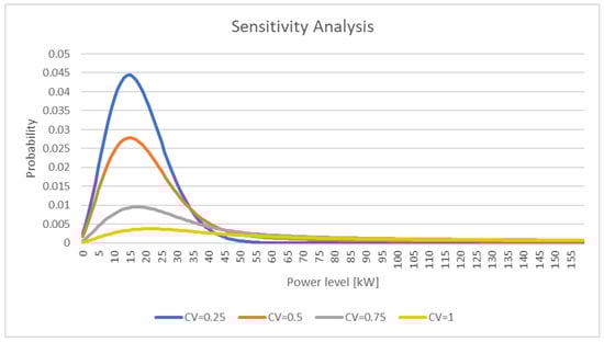
Figure 6.
Probability distributions of the states (Power levels) varying the CV value for the Mx/M/∞ model.
The following Table 7 shows the different service level values depending on the CV value. The calculation of the service level is referred to as the same value as the power of the previous example.
Table 7.
Service level varying the CV value for the Mx/M/∞ model.
When considering greater variability in power consumption (i.e., variability in the size of the arrival lot), the deterioration of the service level at an equal power level is evident. The values of CV considered in this analysis are very high, e.g., when CV = 1, the standard deviation equals the mean of the normal distribution. However, this analysis highlights the importance of the accurate assessment of the variability of energy consumption, as the impact of the latter is not negligible.
5. Discussions and Conclusions
The rising costs associated with energy and the push to minimise environmental impact must be matched by greater attention in the study of energy consumption. This paper provides an analytical method based on stochastic distributions to dynamically model the power requirements of the system. Therefore, the proposed method is meant to be a design tool useful for the evaluation of the power requirements of the system under-sizing and not a method for energy operational management and monitoring. In this way, it is possible to support managerial decisions for both the definition of the energy supply contract and production planning by providing an assessment of power requirements. Specifically, the proposed method stands as an alternative/complement to the traditional method based on the static notions of load factor and coincidence factor. The strength of the method based on queuing theory is the probabilistic and dynamic view of the system, which, in addition to the presence of an analytical formulation, makes it possible to study different scenarios and predict power requirements. In addition, the possibility to calculate the service level associated with a given power level allows economic evaluations, such as considering possible penalties for exceeding the contracted power level. Moreover, the ability to assess the variability of machine consumption through the probability distributions of the arrival batch (i.e., through the Mx/M/∞ model) enables the exploration of a wide range of scenarios from the most optimistic to the most pessimistic. Comparing the results yielded by the three different models highlights the importance of an in-depth study of energy consumption; in fact, the simplest model (i.e., M/M/∞) provides results that differ significantly from the more complex models both in terms of probability distributions and service level. In order for this method to be used reliably, it would be necessary to study a variety of different industrial cases to evaluate the goodness of the results, but in any case, it remains possible to use this method as support or comparison with the traditional approach.
Author Contributions
Conceptualization, I.F.; Data curation, M.C.; Methodology, I.F. and M.C.; Validation, M.C.; Writing—original draft, M.C.; Writing—review & editing, I.F. and L.E.Z. All authors have read and agreed to the published version of the manuscript.
Funding
This research received no external funding.
Data Availability Statement
The authors confirm that the data supporting the findings of this study are available within the article.
Conflicts of Interest
The authors declare no conflict of interest.
References
- Zanoni, S.; Zavanella, L.E.; Ferretti, I. Energy value stream methods with auxiliary systems. In Proceedings of the ECEEE Industrial Summer Study on Industrial Efficiency: Leading the Low-Carbon Transition, Kalkscheune, Berlin, Germany, 11–13 June 2018; pp. 281–291. [Google Scholar]
- Zanoni, S.; Ferretti, I.; Zavanella, L.E. Energy savings in reheating furnaces through process modelling. Procedia Manuf. 2020, 42, 205–210. [Google Scholar] [CrossRef]
- Zavanella, L.; Zanoni, S.; Ferretti, I.; Mazzoldi, L. Energy demand in production systems: A Queuing Theory perspective. Intern. J. Prod. Econ. 2015, 170, 393–400. [Google Scholar] [CrossRef]
- Ferretti, I.; Zavanella, L.E. Batch Energy Scheduling Problem with no-wait / blocking Constraints for the general Flow-shop Problem. Procedia Manuf. 2020, 42, 273–280. [Google Scholar] [CrossRef]
- Zavanella, L.; Zanoni, S.; Marchi, B.; Ferretti, I. Energy considerations for the economic production quantity and the joint economic lot sizing. J. Bus. Econ. 2019, 89, 845–865. [Google Scholar] [CrossRef]
- Ferretti, I.; Zanoni, S.; Zavanella, L.E. Energy efficiency in a steel plant using optimization-simulation. In Proceedings of the 20th European Modeling and Simulation Symposium, EMSS 2008, Amantea, Italy, 17–19 September 2008; pp. 180–187. [Google Scholar]
- Gan, S.; Kang, L.; Wang, Y.; Cameron, C. IoT based energy consumption monitoring platform for industrial processes. In Proceedings of the 2018 UKACC 12th International Conference on Control (CONTROL), Sheffield, UK, 5–7 September 2018. [Google Scholar]
- Mudaliar, M.D.; Sivakumar, N. Internet of Things IoT based real time energy monitoring system using Raspberry Pi. Internet Things 2020, 12, 100292. [Google Scholar] [CrossRef]
- Dietmair, A.; Verl, A. A generic energy consumption model for decision making and energy efficiency optimisation in manufacturing. Int. J. Sustain. Eng. 2009, 2, 123–133. [Google Scholar] [CrossRef]
- Mouzon, G.; Yildirim, M.B.; Twomey, J. Operational methods for minimization of energy consumption of manufacturing equipment. Int. J. Prod. Res. 2007, 45, 4247–4271. [Google Scholar] [CrossRef]
- Bruzzone, A.A.G.; Anghinolfi, D.; Paolucci, M.; Tonelli, F. Energy-aware scheduling for improving manufacturing process sustainability: A mathematical model for flexible flow shops. CIRP Ann.-Manuf. Technol. 2012, 61, 459–462. [Google Scholar] [CrossRef]
- Prabhu, V.V.; Jeon, H.W.; Taisch, M. Modeling Green Factory Physics—An Analytical Approach. In Proceedings of the 2012 IEEE International Conference on Automation Science and Engineering (CASE), Seoul, Korea, 20–24 August 2012; pp. 6–11. [Google Scholar]
- Fernandez, M.; Li, L.; Sun, Z. ‘Just-for-Peak’ buffer inventory for peak electricity demand reduction of manufacturing systems. Int. J. Prod. Econ. 2013, 146, 178–184. [Google Scholar] [CrossRef]
- Zanoni, S.; Bettoni, L.; Glock, C.H. Energy implications in a two-stage production system with controllable production rates. Int. J. Prod. Econ. 2014, 149, 164–171. [Google Scholar] [CrossRef]
- Liu, Y.; Dong, H.; Lohse, N.; Petrovic, S. A multi-objective genetic algorithm for optimisation of energy consumption and shop fl oor production performance. Int. J. Prod. Econ. 2016, 179, 259–272. [Google Scholar] [CrossRef]
- Gong, X.; Van Der Wee, M.; De Pessemier, T.; Colle, D.; Martens, L.; Joseph, W. Integrating labor awareness to energy-ef fi cient production scheduling under real-time electricity pricing: An empirical study. J. Clean. Prod. 2017, 168, 238–253. [Google Scholar] [CrossRef]
- Addisu, A.; Badis, H.; George, L. Demand response scheduling in industrial asynchronous production lines constrained by available power and production rate. Appl. Energy 2018, 230, 1414–1424. [Google Scholar]
- Beck, F.G.; Biel, K.; Glock, C.H. Integration of energy aspects into the economic lot scheduling problem. Int. J. Prod. Econ. 2019, 209, 399–410. [Google Scholar] [CrossRef]
- Masmoudi, O.; Delorme, X.; Gianessi, P. Job-shop scheduling problem with energy consideration. Int. J. Prod. Econ. 2019, 216, 12–22. [Google Scholar] [CrossRef]
- He, Y.; Liu, B.; Zhang, X.; Gao, H.; Liu, X. A modeling method of task-oriented energy consumption for machining manufacturing system. J. Clean. Prod. 2012, 23, 167–174. [Google Scholar] [CrossRef]
- Materi, S.; Renna, P. A dynamic decision model for energy-ef fi cient scheduling of manufacturing system with renewable energy supply. J. Clean. Prod. 2020, 270, 122028. [Google Scholar] [CrossRef]
- Luis, J.; Duarte, R.; Fan, N.; Jin, T. Multi-process production scheduling with variable renewable integration and demand response. Eur. J. Oper. Res. 2020, 281, 186–200. [Google Scholar]
- Cheng, L.; Tang, Q.; Zhang, L.; Meng, K. Mathematical model and enhanced cooperative co-evolutionary algorithm for scheduling energy-efficient manufacturing cell. J. Clean. Prod. 2021, 326, 129248. [Google Scholar] [CrossRef]
- Wójcicki, J.; Tolio, T.; Bianchi, G. Cross-level model of a transfer machine energy demand using a two-machine generalized threshold representation. J. Manuf. Syst. 2021, 58, 44–58. [Google Scholar] [CrossRef]
- Zhao, J.; Xue, Z.; Li, T.; Ping, J.; Peng, S. An energy and time prediction model for remanufacturing process using graphical evaluation and review technique (GERT) with multivariant uncertainties. Environ. Sci. Pollut. Res. 2021. [Google Scholar] [CrossRef] [PubMed]
- Cromie, M.V.; Chaudhry, M.L.; Grassmann, W.K. Further Results for the Queueing System Mx/M/c. J. Oper. Res. Soc. 1979, 30, 755–763. [Google Scholar] [CrossRef]
- Eick, S.G.; Massey, W.A.; Whitt, W. The Physics of the Mt/G/∞ Queue. Oper. Res. 1993, 41, 731–742. [Google Scholar] [CrossRef]
- Daw, A.; Pender, J. On the distributions of infinite server queues with batch arrivals. Queueing Syst. 2019, 91, 367–401. [Google Scholar] [CrossRef]
- IEC 60439-1; Low-Voltage Switchgear and Control Gear Assemblies—Part 1: Type-Tested and Partially Type-Tested Assemblies. IEC: Geneva, Switzerland, 2004.


Publisher’s Note: MDPI stays neutral with regard to jurisdictional claims in published maps and institutional affiliations. |
© 2022 by the authors. Licensee MDPI, Basel, Switzerland. This article is an open access article distributed under the terms and conditions of the Creative Commons Attribution (CC BY) license (https://creativecommons.org/licenses/by/4.0/).