Abstract
The main purpose of the work was examining various methods of decomposition of a network optimization problem of simultaneous routing and bandwidth allocation based on Lagrangian relaxation. The problem studied is an NP-hard mixed-integer nonlinear optimization problem. Multiple formulations of the optimization problem are proposed for the problem decomposition. The decomposition methods used several problem formulations and different choices of the dualized constraints. A simple gradient coordination algorithm, cutting-plane coordination algorithm, and their more sophisticated variants were used to solve dual problems. The performance of the proposed decomposition methods was compared to the commercial solver CPLEX and a heuristic algorithm.
1. Introduction
As the latest reports say [1,2], during the first wave of the COVID-19 pandemic in the spring months of 2020, the global Internet traffic increased by almost 40%. This growth was prompted by telecommuting, sharp demand for video conferencing, online gaming, video streaming and social networking. It means that at the beginning of the pandemic crisis there was quite a big capacity surplus in almost all networks. In the same 2020 year, data transmission networks consumed 260–340 TWh or 1.1–1.4% of global electricity use [1]. It is expected that a strong growth in demand for the data centre and network services will continue at least until the end of this decade [3], particularly because of video streaming and gaming. For example, in 2022, they are supposed to make up 87% of consumer Internet traffic [1]. On the other hand, at the beginning of 2022, a global energy crisis has started and we have been observing unprecedented increase in electricity and energy commodities prices and the threat of their shortages. All this makes it more important than ever to use the network infrastructure efficiently to guarantee the highest possible quality of service with the lowest possible energy consumption.
The optimization problem taking into account these two criteria: a penalty for not achieving the eligible flow rates for connections and the total links cost was first formulated by Gallager and Golestaani as early as in 1980 [4]. The deep analysis of this model can be found in [5]. The authors assumed there a multi-path routing and transformed the problem to a standard multicommodity flow problem, which in the convex case could be solved efficiently by any continuous, nonlinear solver. Unfortunately, this approach is not applicable to modern data networks, since such networks have, as a rule, high fixed energy costs (even at low utilisation) and the link power cost cannot be well described by means of a continuous function [1]. Such more realistic formulations with binary variables have been presented in the last years in a connection with energy-aware aka green networks idea [6,7,8,9,10,11,12,13].
The first works on two-criteria network control, optimizing simultaneously both routing and flow rates, appeared in the 1990s [14,15,16]. Because routing variables are binary, these problems are of mixed-integer type, which means that they are NP-hard and as such for larger networks they require specialized suboptimal, heuristic algorithms to obtain an approximate solution in time acceptable for online application. Such methods were presented in the multi-path case in the papers [17,18,19] and in the single-path case in [14,15,16,20,21], all for the linear objective function case. Quite often, these heuristics used Lagrangian relaxation of the problem.
The precise model for quadratic problems, to be solved by a mixed-integer quadratic programming (MIQP) solver, such as CPLEX or Gurobi, was presented in the paper [22]. Unfortunately, the time of solving this problem and obtaining the exact solution is unacceptable in real-time systems. In this paper, the authors are trying to find an algorithm that delivers an approximate solution in short time.
This paper studies and analyzes different methods allowing for decomposing mixed-integer constrained nonlinear optimization problems using Lagrangian relaxation. Decomposition methods solve large-scale problems by splitting them into several smaller subproblems [23,24,25]. In most cases, they exploit the special structure of an optimization problem. A simple decomposable problem structure contains several independent subproblems, which are coupled with constraints and, as a result, the problem can be solved with a lower computational cost, since subproblems are usually much easier to solve than the original problem; moreover, the independence of these subproblems allows for a parallel solution.
Lagrangian relaxation was selected as a general decomposition technique allowing for transforming a problem having an additively separable form [23,24,26]. Usually, in discrete or mixed-integer nonlinear programming (MINLP), Lagrangian relaxation is used to retrieve a tight estimate of the optimal objective, and further this estimate can be used in a combination with other methods such as branch-and-bound. As a result of decomposition methods’ application, one obtains several independent subproblems (so-called local problems) and the master problem. They are solved iteratively, and the master problem provides parameters for local problems. These parameters are Lagrange multipliers. A deep study on the effectiveness of different optimization algorithms at the master level is presented in [21]. In the last decade, Lagrangian relaxation became a very popular approach to find a near-optimal solution in many practical MINLP problems, including: production planning [27,28], ecology [29], the electrical power industry [30], water distribution [31], supply chain networks [32,33,34], transportation [35,36], communication networks [37,38,39], and service systems [40].
In our work like in [21], both different versions of relaxations (dualizations) are analyzed and different approaches to solve the master (coordination) problem are used. We generalize the model from [16,21] because we analyze problems with a nonlinear cost function corresponding to QoS. One of our demand relaxations is quite similar to that of [16,21], but we do not dualize mixed constraints concerning individual arcs, what reduces the dimension of the coordination (dual) problem.
The paper is organized in the following way: Section 2 presents in detail a problem of simultaneous routing and bandwidth allocation in green networks, Section 3 discusses a general decomposition framework used in the paper, Section 4 contains detailed information about several approaches to the decomposition of the problem formulations presented in Section 2. In Section 5, coordination algorithms are introduced, and the results of the numerical tests for the decomposition methods are presented in Section 6. Section 7 summarizes and discusses the results.
2. Problem Formulation
The problem of the simultaneous routing and flow rate optimization can be described as finding single path routing and flow rates’ values satisfying network constraints for every source–destination pair [22].
The following items are used in the mathematical formulation of the problem:
| - | set of all network nodes and a single node, respectively; | |
| - | set of all network arcs and a single arc, respectively; | |
| - | network (graph) for which the optimization problem is formulated; | |
| - | set of all labeled links and a single labeled link, respectively; | |
| - | one-to-one mapping from arcs to links labeled by a single natural number; | |
| - | set of all demands and a single demand, respectively; | |
| - | source and destination node for the specific demand w, respectively; | |
| - | flow rate for the specific demand w, , | |
| - | lower and upper bound on the flow rate for the demand w, we assume that ; | |
| - | capacity of the link l; | |
| - | binary routing decision variable, whether the link l is used by the demand w; | |
| - | positive parameter—weight of the QoS part of the objective function; | |
| - | positive parameter—weight of the energy usage part of the objective function, |
The problem can be formulated in the following way [22]:
subject to
The above formulation will be later referred to as P. Objective function (1) is quadratic and convex. The first term is a Quality of Service component and expresses a cost for not delivering the full bandwidth for all connections . The second term expresses the total cost of energy used in the network and is proportional to the number of used links. The detailed description of this problem can be found in [22]. Other nonlinear, and even nonconvex, components of P are constraints (5). Because of the simultaneous usage of the binary variables and continuous variables , this optimization problem has a mixed domain. It means that P belongs to the MINLP class of the optimization problems and as such is NP-hard.
2.1. Linearized Constraints
The products of continuous and binary variables in nonlinear constraints (5), which are nonconvex functions, can be replaced with auxiliary variables and several additional linear constraints [22]. The new, added linear constraints ensure fulfillment of the following equality:
The optimization problem formulation with linearized constraints is presented below; this problem will be later referred to as :
subject to
Originally, constraints (12) and (15) used an arbitrarily selected so-called Big M number, that is a constant of a much higher order than the data of the problem [22], but, according to [41], replacing it with a smaller value may allow for achieving better numerical results. Thus, M was replaced with —the upper bound on the flow rate .
2.2. Alternative Problem Formulation
An alternative problem formulation inspired by [42] may be proposed. This formulation still utilizes variables , but in this case flow conservation law Equations (2) are expressed with auxiliary variables . This problem formulation will be later referred to as :
subject to
Constraints (20) force single path routing; constraints (23) keep the relationship between auxiliary variables and binary variables. Formulation is equivalent to and P provided that .
3. Lagrangian Relaxation
Lagrangian relaxation is one of the most popular relaxation methods [23,24]. In short, it consists in the replacement of the original optimization problem:
subject to:
where , with a two-step problem
The function is called the Lagrange function or Lagrangian, the function is called the dual function, the vectors , are called Lagrange multipliers. The external optimization in (27) is usually solved iteratively.
The theory says [43] that, if the set X is a convex subset of , the functions are convex over X, the functions are affine, the optimal value is finite and there exists a vector such that , then there exist Lagrange multipliers such that the solutions of the primal (24)–(26) and the dual problem (27) are equal.
Lagrangian relaxation is particularly useful when the functions f and g are separable, that is, they can be expressed as the sums of the components dependent on the same separate subvectors of x, and the set X is a Cartesian product of the sets from spaces of the same subvectors. Such a structure of the optimization problem allows to approximate a large optimization problem by a set of smaller problems related to the original problem, solved in a loop together with a coordination problem delivering parameters modifying them.
Another example of a relaxation for the MINLP problem is continuous relaxation, which removes the integrality constraint and allows all variables to be real. The solution retrieved from the relaxation can be utilized in the branch-and-bound algorithm to obtain a solution of the original problem.
Lagrangian relaxation relies on constraints relaxation. For some problems having decomposable structure, it may result in significant problem simplification. The value of the dual function is always less than or equal to the optimal value of the primal problem. This property is called weak duality. Some problems may possess yet one property, called strong duality. For the strong duality, the optimal value of the dual problem is equal to the optimal value of the primal problem. The conditions for that are mentioned above. In such a case, Lagrangian relaxation allows for achieving the optimal value of the primal problem via solving the dual problem.
Unfortunately, an MINLP problem analyzed in this work operates on a mixed domain and only weak duality holds. It means that Lagrangian relaxation is able to provide only the lower bound to the primal problem.
Bounds provided by the Lagrangian relaxation are often used in conjunction with the branch-and-bound algorithm, and used in the same way as in the case of the continuous relaxation. However, usually Lagrangian relaxation provides tighter bounds than continuous relaxation [23]. At this point, it is important to introduce relations between primal optimal solution and dual optimal solution and their optimal decision variables.
Duality gap is the difference in the optimum between primal and dual problems’ objectives. It was noticed that in many practical problems the duality gap is vanishing when the number of variables grows. Evaluation of the duality gap is described in detail and proven in [44]. First of all, the duality gap depends on the number of relaxed constraints. This dependence can be described by the inequality:
where represents the optimal value of the primal problem objective function, represents the optimal value of the dual problem objective function and is the duality gap. The number of relaxed constraints is denoted by m and E is a parameter that depends on the problem objective function and its constraints specific properties. The estimation presented above is valid only if a list of assumptions is fulfilled [44]. Fortunately, the problem studied in this work satisfies these assumptions. We attempt to utilize the solution of the dual problem using special structure of the studied problem P. It allows for easy retrieving the feasible solution for situations when capacity constraints (5) were violated, but paths defined by routing variables still remain feasible. The method of retrieving such a feasible solution is described in Section 6.1 as a part of the heuristic algorithm.
4. Decomposition Methods
4.1. Demands Decomposition
The most obvious approach to apply Lagrange relaxation is based on the relaxation of the capacity constraints binding flows. There is no sense to consider the formulation P because of nonconvexity of the capacity constraints (5). Fortunately, for both and formulations, capacity constraints are represented by the same convex functions, respectively (11) and (21).
The Lagrange function for both and problems is as follows:
It is separable and, by changing the order of summation operators, we can write it as:
The dual function for the problem is:
subject to (8)–(10) and (12)–(15).
Since, in the optimization problem (31), constraints (8)–(10) and (12)–(15) can be partitioned with respect to different flows into completely independent, the minimization there can be performed independently for components dependent on particular flows w with respect to corresponding decision variables. That is, the dual function for problem can be calculated in the following way:
where
subject to
The dual function for problem is defined as the optimization problem with the same objective function as for the problem , but with different constraints, that is:
subject to (17)–(20) and (22)–(23).
In the same way as for the problem , it may be calculated as follows:
where the component functions are
subject to:
The dual problem for formulations can be presented, respectively, as:
and
As it can be seen from the formulations presented above, in both cases, the problem was decomposed and the minimization, which is performed to determine the dual function, can be done independently for every demand .
Such a structure was achieved by the relaxation of the coupling capacity constraints. The number of relaxed constraints is equal to . The number of variables presented in the studied problem, when no artificial variables were used, is equal to . When were used, the number of variables is equal to . Hence, the relation of the number of relaxed constraints to the number of variables is acceptable.
Because capacity constraints were relaxed, optimal decision variables of the local problems may violate them. However, fortunately, the method of optimal feasible flow rate allocation, described in Section 6.1, can be applied for routes retrieved from the problem solution, to find a feasible solution.
4.2. Subnetworks Decomposition
Subnetworks decomposition is based on distinguishing subgraphs in the problem graph . These subgraphs, also called subnetworks, are selected groups of nodes, loosely connected with other nodes. The less the subnetwork is connected with other subnetworks, the tighter relaxation will be (that is, with the smaller number of the relaxed constraints). The new problem formulations presented in this subsection introduce subnetworks . Every node belongs exactly to one subnetwork; arcs can belong to one or two subnetworks. Arcs which belong to a pair of subnetworks are duplicated for every subnetwork, and this encompasses their labeled links and flow rates. All duplicated components must be equal for keeping this formulation valid.
The following additional components are used in a mathematical problem description for the subnetworks decomposition, which is an adaptation of the original problems or :
| - | division of a given network | |
| into S subnetworks that is ; this is not a partition because of common links on the borders (see below), | ||
| - | set of all nodes of a subnetwork - this is a partition of the set N that is: , | |
| - | set of all arcs of a subnetwork | |
| - | set of internal arcs of the subnetwork | |
| - | set of all labels of links of a subnetwork | |
| - | flow rate for the demand w in the subnetwork | |
| - | binary routing variable for the flow w in the subnetwork and link | |
| - | set of external arcs (incoming or outgoing) | |
| of the subnetwork | ||
| - | indices of subnetworks directly connected | |
| with | ||
| - | set of labels of external links for the subnetwork | |
| - | correcting coefficient to avoid adding external arcs twice. |
Now, the problem can be formulated in the following way:
subject to
The problem will obtain the form:
subject to
Connections between subnetworks do not allow for solving problems independently for every subnetwork . Internetwork connections correspond to the duplicated flow rates and routing variables equalities (54) and (55) or (65) and (66), so these constraints should be relaxed to achieve decomposable structure.
The Lagrange function for the and problems is the following:
where for are Lagrange multipliers.
The dual function for the problem can be calculated as:
subject to (53), (56)–(62), where the function is given by (75).
The dual function components can be calculated independently for every subnetwork because all constraints representing connections between subnetworks have been relaxed. The number of the relaxed constraints depends on the number of subnetworks S and on the number of connections between them. These constraints have to be relaxed for every demand .
4.3. Continuous and Binary Variables Decomposition
Decomposition presented in this subsection splits the original MINLP problem into two subproblems: the first containing only continuous variables and the second containing only binary variables. Such decomposition can be performed for both problem formulations and .
Continuous and binary variables decomposition is achieved by relaxing constraints containing binary and continuous variables simultaneously, that is, constraints (12), (15) for and (23) for . The Lagrange function for the problem will be:
The dual function for the problem with the separation of continuous and binary variables is calculated in the following way:
where
subject to
and
subject to
After decomposition, the dual function consists of two parts: the first contains continuous variables, the second contains binary variables. The binary part of the dual function consists of the linear objective function and network flow conservation law rule (86). These constraints can be presented by a unimodular matrix. As a result, has an integrality property, that is, the problem decision variables at the optimum are always integer. Thus, the constraints (10) preserving that the route variables are binary can be safely omitted. Hence, the decomposed problem does not operate on the mixed domain.
Unfortunately, the number of relaxed constraints is rather big—. It may result in unsatisfactory tightness of the relaxation.
The Lagrange function for the problem with a separation of continuous and binary variables is:
The dual function for the problem with the separation of continuous and binary variables is following:
where
subject to
and
subject to
For the alternative problem formulation (16)–(23), continuous and binary variable decomposition requires the relaxation of constraints (23). The number of the relaxed constraints in this case is equal to . However, the binary subproblem does not possess integrality property in this case. In addition, violations of the relaxed constraints (23) violate the relation between routing variables and auxiliary variables , which can result in the violations of network flow balance constraints (2). Thus, the following conclusions can be made: decomposition of allows for getting tighter bounds than decomposition of , but subproblems of the decomposed are harder to solve than subproblems of the decomposed .
5. Coordination Algorithms
A dual problem is solved iteratively. In every iteration for given Lagrange multipliers, a dual function is computed (local problem) and Lagrange multipliers are updated (the coordination problem). Several coordination algorithms were used to solve the dual problems presented in the previous section.
- 1.
- Simple gradient algorithmsA simple gradient algorithm to update Lagrange multipliers directly uses the gradient of the dual function, in the following manner:
- For multipliers of the relaxed equality constraints:
- For multipliers of the relaxed inequality constraints:
Parameter (k - iteration number) plays a key role in the simple gradient coordination algorithm. It is responsible for the algorithm convergence rate. Some simple methods for parameter computation can be used [45]:- Square summable, but not summable:
- Nonsummable diminishing:
More sophisticated techniques for evaluation can also be used. Some of them utilize knowledge of the optimal objective value (or its estimate). One of the most advanced methods is Goffin and Kiwiel’s algorithm of the simultaneous optimal value estimation and Lagrange multipliers update [46], which guarantees convergence with an acceptable rate and relatively easy tuning of parameters. This very version of the simple gradient coordination algorithm has been used in our numerical tests.The simple gradient algorithm is strongly dependent on its parameters. Quite often, its convergence rate can be unsatisfactory. However, this algorithm is relatively easy to implement and requires rather small computational efforts. Hence, for a large number of the Lagrange multipliers, this coordination method may be the most appropriate. - 2.
- Cutting plane methodCutting plane algorithms also utilize dual function gradients, but in a different way than simple gradient algorithms. Namely, the approximation of the dual function is based on the dual function gradient in the following manner (for simplicity, we assume that the problem has only inequality constraints):The approximated dual problemcan be reformulated as:In the cutting plane algorithm, dual function approximation is built iteratively. New cuts, defined by linear functions which use dual function gradients, are added in every iteration. The solution of the approximated dual problem is a point where the new cut will be put. It means that, with every iteration, a better piecewise linear approximation of the dual function is achieved. And then, in every iteration of the algorithm, the optimization problem described by (105)–(107) is solved.A similar, but more sophisticated algorithm (which will be used in numerical tests) can also be applied to approximate the dual function and to solve the dual problem [47]. Namely, the dual function can be formulated in the following manner:In the case of the (108) formula, a penalty component was added to keep a stable convergence rate of the algorithm. Two kinds of steps are described in [47] for the algorithm. The first is a significant step: , the second is zero-step: . Zero step still uses new Lagrange multipliers to build a better approximation, but does not update a penalty parameter, so it allows for achieving a better approximation. Meanwhile, a significant step requires significant reduction of the dual value and is performed when:where parameter . The problem of the inactive cuts gathering is also solved in [47]. They can be safely removed from the dual problem formulation when Lagrange multipliers of inactive cuts are equal to zero. Thus, after solving the approximated dual problem (108) in every iteration, Lagrange multipliers of the cuts (106)–(107) are retrieved and only cuts with nonzero Lagrange multipliers are kept; those remaining are removed.To summarize, cutting plane methods are more complicated and require more computational effort for solving an additional optimization problem in every iteration. The problem considered in this paper may become rather complicated for a greater number of Lagrange multipliers. Fortunately, this method allows for achieving a more precise result and is almost independent of parameters tuning.
6. Numerical Tests
The methods described above were studied and tested on several problems. Networks of different sizes were generated with the sets of demands defined for them. Then, the problems of simultaneous routing and flow allocation were formulated for these networks. The tested networks consist of multiple nodes clusters, which are loosely connected. However, nodes inside the clusters are strongly connected. Such network configuration allows for performing subnetworks decomposition relaxing a relatively small number of constraints.
First, problems P were solved by an MINLP solver to obtain optimal solutions. Then, decomposition methods based on Lagrangian relaxation were applied to them. Multiple local problems obtained from decompositions were solved sequentially (can be solved in parallel), and the selected coordination algorithm updated Lagrange multipliers. The process of solving local problems and updating Lagrange multipliers for them was performed iteratively until a stop condition was met. All combinations of the Lagrangian relaxation based decomposition methods and coordination algorithms were studied.
Finally, a simple heuristic method, namely a Heuristic Routes Finding (HRF) algorithm presented below, was applied to solve these optimization problems in a decomposed manner.
All implementations and numerical tests were performed using a Python programming language. Pyomo software package was used to formulate and analyze optimization problems. The following optimization software packages were used: CPLEX (local problems solver, primal problem solver, R problem of the heuristic algorithm solver) and IPOPT (coordination problem solver). A NetworkX software package was used to generate and visualize optimization problems’ networks.
6.1. Simple Heuristic Routes Finding (HRF) Algorithm
Heuristic methods do not guarantee achieving the optimal solution. However, such methods may allow solving problems at lower costs. Article [48] describes and improves a certain heuristic method for solving the optimization problem of the simultaneous routing and flow bandwidth allocation. The heuristic approach presented there separates the routing problem and flow rate allocation. First, the weight of every arc is calculated as the minimum of capacity for a given link and flow rate upper bound to prevent flow rates’ upper bound violations. Then, the Dijkstra shortest path algorithm is applied to every demand w, that is, for every pair of source and destination nodes, the optimal path is calculated. In the second step, for known optimal paths (routes) , the following flow allocation problem is solved as a continuous nonlinear programming problem:
subject to
6.2. Generation of Networks
For numerical tests, two network topologies were generated: the first with a lower number of variables (referred to as a medium network)—see Table 1 and Figure 1 and the second with a greater number of variables (referred to as a large network)—see Table 2 and Figure 2. Five seeds were used to formulate randomized problem instances. For every problem instance, the source and the destination nodes were generated randomly, and so were the capacities of links. Problem instances were generated for both network topologies. Several approaches to optimization problem formulation were used. Networks and their parameters, the results of network decomposition achieved with HRF heuristics and the results achieved with several Lagrange decomposition methods (in combination with two coordination algorithms) will be presented in this section.

Table 1.
Medium problem instances’ parameters.
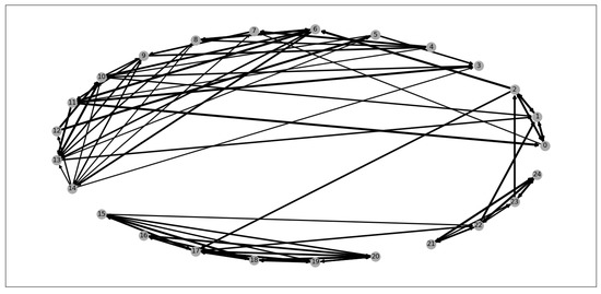
Figure 1.
Medium network topology.
Table 2.
Large problem instances’ parameters.
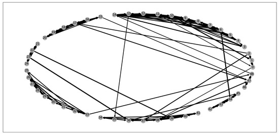
Figure 2.
Large network topology.
6.3. Comparison of Results for Different Methods
The numerical tests were made only for formulations and (which differ in flow conservation equations using, respectively, binary or continuous variables) because the only nonlinear component in these formulations is a convex quadratic part of the objective function. Meanwhile, the formulation P has nonconvex constraints, which complicate solving the problem. All three decomposition approaches that is: demand, subnetworks and binary/continuous variables were checked.
Numerical experiments were performed according to the following scenario: first, the CPLEX solver attempted to solve all problem formulations; then, all decomposition methods were applied; finally, a feasible solution was restored if it was possible.
The following items are used to describe the results of computations:
| Objective | —value of the problem objective function, |
| Spent Time | —time spent to retrieve solutions in seconds, |
| Feasibility | —solution feasibility validation (for the original problem P); for infeasible solution number of capacity constraints (5) violations—“CCV: <number>”, and number of routing constraints (2) violations |
| —“RCV: <number>”, | |
| Status | —solution status retrieved from a solver, |
| Dual Objective (LB) | —value of the dual problem objective function, which is also a lower bound for the primal problem, |
| Heuristic Objective (LB) | —value of the problems objective function retrieved using the HRF Algorithm, |
| Reallocated (UB) | —value of a feasible solution restored from a lower bound solution routing variables using solution of the R problem, which is also an upper bound for the primal problem, |
| LB Relative Gap | —ratio of the lower bound gap with respect to the optimal objective given in percents () |
| UB Relative Gap | —ratio of the upper bound gap with respect to the optimal objective given in percents () |
The tests were performed on the machine with Intel Core i7-4710 HQ, 4 core 2.5–3.5 GHz processor, 16 GB of DDR3-1600, dual-channel memory and 512 GB SSD storage, under Ubuntu 18.04 operating system. As it was said before, every numerical test was executed for five randomly generated problem instances.
The results of optimization obtained by CPLEX solver for medium-sized networks are presented in Table 3. These results will serve further as a benchmark for us. In particular, the gaps are calculated in relation to them.
Table 3.
Numerical results for medium problems—CPLEX solver.
The average results of tests of different decomposition approaches are presented in Figure 3, Figure 4 and Figure 5; the detailed results for all medium-sized networks in Table 4, Table 5, Table 6 and Table 7.
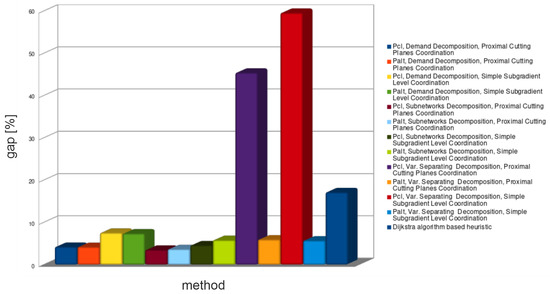
Figure 3.
Average lower bound relative gap for all decomposition methods—medium problems.
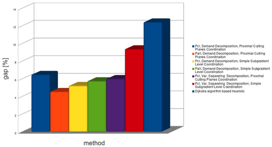
Figure 4.
Average upper bound relative gap for all decomposition methods—medium problems.
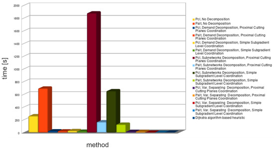
Figure 5.
Average spent time for all decomposition methods—medium problems.
Table 4.
Numerical results for medium problems—demands decomposition.
Table 5.
Numerical results for medium problems—subnetworks decomposition.
Table 6.
Numerical results for medium problems—continuous and binary variables decomposition.
Table 7.
Numerical results for medium problems—Dijkstra algorithm based heuristics (HRF).
The demands decomposition method (see Table 4) solved almost all medium problem instances in a shorter time than CPLEX. Solutions obtained from this method provide problem lower bounds—relative gaps of these solutions are within the range: 3–11%. Unfortunately, all retrieved solutions violated capacity constraints. Feasible solutions (upper bounds) obtained from the lower bounds’ routings are within the range: 3–13%. Importantly, tighter lower bounds did not always provide tighter upper bounds.
Subnetworks decomposition (see Table 5) spent an unacceptable amount of time to find solutions for almost all medium-sized problem instances (decomposed problem was solved much longer than the primal problem). Spent time of formulations is much shorter than that of formulations, but still unsatisfactory. Lower bounds provided by subnetworks decomposition are the tightest: 1–7.5%. Unfortunately, all solutions retrieved from this decomposition violated routing constraints. Because of that, as well as because of unacceptable spent times, subnetwork decomposition was not applied to large problem instances.
The continuous and binary variables decomposition method (see Table 6) was the quickest from the Lagrangian based decomposition methods. This decomposition method shows how a large number of Lagrange multipliers increases coordination time for cutting planes’ algorithms. As it can be seen, it provides a big duality gap for the formulation . However, the duality gap for this method is small when formulation is used. Unfortunately, such gap is achieved for zero-valued Lagrange multipliers, which means that the bound was not improved (see Figure 6 and Figure 7) by coordination algorithms (zero-valued Lagrange multiplier are the start point of the coordination).
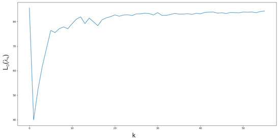
Figure 6.
Dual function value during proximal cutting plane coordination algorithm iterations. Continuous and binary variables decomposition for , medium problem, instance 1.
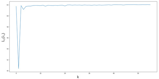
Figure 7.
Dual function value during simple subgradient level method coordination algorithm iterations. Continuous and binary variables decomposition for , medium problem, instance 1.
In addition, feasible solutions (upper bounds) were restored from routings obtained from continuous and binary variable decomposition for formulation . The tightness of these solutions is comparable to the demand decomposition solutions, regardless of the large duality gap.
The undesirable properties of continuous and binary variable decomposition method are derived from a large number of relaxed constraints—comparable to the number of variables. Because of such unsatisfactory results for medium networks, the continuous and binary variables decomposition method was not used in further numerical tests.
The heuristic method (see Table 7) was not able to provide neither tight lower bounds nor tight upper bounds. Times spent by this method were very small, but still not small enough to use this method in combination with the branch-and-bound algorithm.
From now on, the results of tests for large problems will be presented.
From Table 8, it is seen that the commercial solver CPLEX was able to find the optimal solutions for only 2 of 10 instances in a time less than 2000 s.
Table 8.
Numerical results for large problems—CPLEX solver.
As it was stated before, only a demands decomposition approach was applied and for comparison of the simple HRF method. The average results are presented in Figure 8, Figure 9 and Figure 10, and the detailed ones in Table 9 and Table 10.
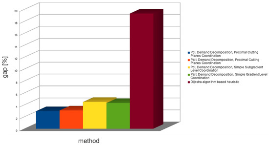
Figure 8.
Average lower bound relative gap for all decomposition methods—large problems.
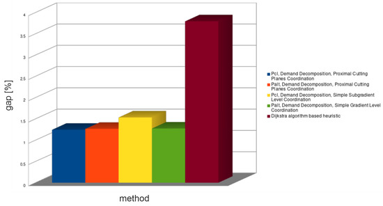
Figure 9.
Average upper bound relative gap for all decomposition methods—large problems.
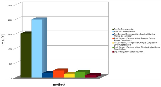
Figure 10.
Average spent time for all decomposition methods—large problems.
Table 9.
Numerical results for large problems—demands decomposition.
Table 10.
Numerical results for large problems—Dijkstra algorithm based heuristics (HRF).
Demands decomposition for large problem instances (see Table 9) was able to provide tighter lower bounds (1–7.4%) than for medium problem instances. Unexpectedly, the obtained upper bounds (0–3%) were also much better than for medium problem instances. Since, as it was stated before, the commercial solver CPLEX failed to find the optimal solutions for most of the instances in half an hour, while the demands decomposition method found solutions in few minutes, it is a very good algorithm for real-time systems.
In the case of large problem instances (see Table 10), lower bound relative gaps for solutions found by the heuristic method are comparable to the gaps for medium problem instances. However, the obtained upper bounds gaps were smaller than for medium problem instances, just as with the demands decomposition. Spent times of the heuristic methods were even shorter than for the demand decomposition.
7. Conclusions
The decomposition methods presented in the paper can approximately solve the problems of simultaneous routing and bandwidth allocation in energy-aware networks with less time expenditure than a commercial solver. The quality of the produced solution is strongly dependent on the problem parameters such as: network topology, number of demands, capacities of links, and flow rate bounds. The selection of the appropriate decomposition method should be connected with finding the most scalable component of the solved problems.
The heuristic method presented in Section 6.1 was the fastest one, but the optimal solution approximation provided by it was not precise enough. Because of that, an attempt to combine this method with a branch and bound algorithm was made. Unfortunately, for large problem instances, this approach failed.
The decomposition methods based on Lagrangian relaxation showed a better precision. As it turned out, their performance may strongly depend on the optimization problem formulation. The quality of the solution is better for decomposition methods with a lower number of relaxed constraints. Because of that, the continuous and binary variables decomposition method did not present well.
The subnetworks decomposition can produce quite a good approximation of the optimal value of the primal problem. Unfortunately, this method did not allow for gaining a satisfactory performance boost for the tested instances—finding local problems solutions could be enormously long. Local problems retrieved from the demand decomposition or the subnetworks decomposition are problems of a smaller size, but still mixed-integer and NP-hard, so their complexity may remain significant. Moreover, the solutions delivered by this method do not form paths, and it is impossible to restore a feasible solution in a simple way.
Meanwhile, the demand decomposition method allowed for retrieving a solution with a relatively small duality gap and made this in a much shorter time than a commercial solver. In addition, in the case of demand decomposition, a local problem solution can be used to restore a solution feasible for the primal problem.
Both coordination algorithms used in tests were able to find the solution of the dual problems. Overall, a cutting plane method with the proximal component provided better solutions, but the simple gradient level method was able to produce comparable solutions in a shorter time. Moreover, cutting planes’ methods need much more time with the growth of the number of Lagrange multipliers, so, for problems involving a large number of multipliers, simple gradient algorithms may deliver a significant performance increase.
Despite the usage of the presented methods for finding the exact solution of the primal problem seems to be not promising, the Lagrangian relaxation decomposition methods for large problem instances are still able to provide a good estimate of the optimal value of the objective function in a much shorter time than a commercial solver finds the optimal solution.
Author Contributions
Conceptualization, A.K.; methodology, I.R., A.K.; software, I.R.; validation, I.R. and A.K.; formal analysis, I.R. and A.K.; investigation, I.R. and A.K.; resources, I.R. and A.K.; writing—original draft preparation, I.R. (except: Section 1—A.K., Section 3, Section 4.2, Section 5 and Section 7—I.R. and A.K.); writing—review and editing, A.K. All authors have read and agreed to the published version of the manuscript.
Funding
This research received no external funding.
Institutional Review Board Statement
Not applicable.
Informed Consent Statement
Not applicable.
Data Availability Statement
Not applicable.
Conflicts of Interest
The authors declare no conflict of interest.
References
- Data Centres and Data Transmission Networks. Available online: https://www.iea.org/reports/data-centres-and-data-transmission-networks. (accessed on 22 August 2022).
- The Growing Footprint of Digitalisation. Available online: https://www.unep.org/resources/emerging-issues/growing-footprint-digitalisation. (accessed on 22 August 2022).
- Koot, M.; Wijnhoven, F. Usage impact on data center electricity needs: A system dynamic forecasting model. Appl. Energy 2021, 291, 116798. [Google Scholar] [CrossRef]
- Gallager, R.; Golestaani, S. Flow Control and Routing Algorithms for Data Networks. In Proceedings of the 5th International Conference on Computer Communication (ICCC 1980), Atlanta, GA, USA, 27–30 October 1980; pp. 779–784. [Google Scholar]
- Bertsekas, D.; Gallager, R. Data Networks, 2nd ed.; Prentice-Hall International, Inc.: Englewood Cliffs, NJ, USA, 1992. [Google Scholar]
- Chiaraviglio, L.; Mellia, M.; Neri, F. Energy-aware backbone networks: A case study. In Proceedings of the 1st International Workshop on Green Communications, IEEE International Conference on Communications (ICC’09), Dresden, Germany, 14–18 June 2009; pp. 1–5. [Google Scholar]
- Mahadevan, P.; Sharma, P.; Banerjee, S.; Ranganathan, P. Energy Aware Network Operations. In Proceedings of the 28th IEEE International Conference on Computer Communications Workshops, INFOCOM’09, Rio de Janeiro, Brazil, 19–25 April 2009; pp. 25–30. [Google Scholar]
- Chiaraviglio, L.; Mellia, M.; Neri, F. Minimizing ISP network energy cost: Formulation and solutions. IEEE/ACM Trans. Netw. 2011, 20, 463–476. [Google Scholar] [CrossRef]
- Zhang, M.; Yi, C.; Liu, B.; Zhang, B. GreenTE: Power-aware traffic engineering. In Proceedings of the 18th IEEE International Conference on Network Protocols (ICNP’2010), Kyoto, Japan, 5–8 October 2010. [Google Scholar]
- Vasić, N.; Kostić, D. Energy-aware traffic engineering. In Proceedings of the 1stInternational Conference on Energy-Efficient Computing and Networking (E-ENERGY 2010), Passau, Germany, 13–15 April 2010. [Google Scholar]
- Bolla, R.; Bruschi, R.; Davoli, F.; Cucchietti, F. Energy Efficiency in the Future Internet: A Survey of Existing Approaches and Trends in Energy-Aware Fixed Network Infrastructures. IEEE Commun. Surv. Tutor. 2011, 13, 223–244. [Google Scholar] [CrossRef]
- Bianzino, A.P.; Chaudet, C.; Rossi, D.; Rougier, J.L. A survey of green networking research. IEEE Commun. Surv. Tutorials 2012, 2. [Google Scholar] [CrossRef]
- Maaloul, R.; Chaari, L.; Cousin, B. Energy saving in carrier-grade networks: A survey. Comput. Stand. Interfaces 2018, 55, 8–26. [Google Scholar] [CrossRef]
- Magnanti, T.; Mirchandani, P.; Vachani, R. The convex hull of two core capacitated network design problems. Math. Program. 1993, 60, 233–250. [Google Scholar] [CrossRef]
- Balakrishnan, A.; Magnanti, T.L.; Mirchandani, P. Dual-based algorithm for multi-level network design. Manag. Sci. 1994, 40, 567–581. [Google Scholar] [CrossRef][Green Version]
- Gendron, B.; Crainic, T.G.; Frangioni, A. Multicommodity Capacitated Network Design. In Telecommunications Network Planning; Sansò, B., Soriano, P., Eds.; Springer: Boston, MA, USA, 1999; pp. 1–19. [Google Scholar]
- Bouras, I.; Figueiredo, R.; Poss, M.; Zhou, F. Minimizing energy and link utilization in ISP backbone networks with multi-path routing: A bi-level approach. Optim. Lett. 2020, 14, 209–227. [Google Scholar] [CrossRef]
- Yazbek, H.; Liu, P. On adaptive multi-objective optimization for greener wired networks. SN Appl. Sci. 2020, 2. [Google Scholar] [CrossRef]
- Yazbek, H.; Liu, P. A Perspective on Stable Wired Networks while Reducing Energy Use with Load Balance. In Proceedings of SoutheastCon 2022 Conference, SOUTHEASTCON 2022, Mobile, AL, USA, 26 March–3 April 2022; pp. 23–30. [Google Scholar]
- Niewiadomska-Szynkiewicz, E.; Sikora, A.; Arabas, P.; Kołodziej, J. Control system for reducing energy consumption in backbone computer network. Concurr. Comput. Pract. Exp. 2012, 25, 1738–1754. [Google Scholar] [CrossRef]
- Frangioni, A.; Gendron, B.; Gorgone, E. On the computational efficiency of subgradient methods: A case study with Lagrangian bounds. Math. Program. Comput. 2017, 9, 573–604. [Google Scholar] [CrossRef]
- Jaskóła, P.; Arabas, P.; Karbowski, A. Simultaneous routing and flow rate optimization in energy-aware computer networks. Int. J. Appl. Math. Comput. Sci. 2016, 26, 231–243. [Google Scholar] [CrossRef]
- Nowak, I. Relaxation and Decomposition Methods for Mixed Integer Nonlinear Programming; Birkhäuser: Basel, Switzerland, 2005. [Google Scholar]
- Li, D.; Sun, X. Nonlinear Integer Programming; Springer: New York, NY, USA, 2006. [Google Scholar]
- Karbowski, A. Generalized Benders decomposition method to solve big mixed-integer nonlinear optimization problems with convex objective and constraints functions. Energies 2021, 14, 6503. [Google Scholar] [CrossRef]
- Lee, J.; Leyffer, S. Mixed Integer Nonlinear Programming; Springer: New York, NY, USA, 2012. [Google Scholar]
- Mouret, S.; Grossmann, I.; Pestiaux, P. A new Lagrangian decomposition approach applied to the integration of refinery planning and crude-oil scheduling. Comput. Chem. Eng. 2011, 35, 2750–2766. [Google Scholar] [CrossRef]
- Tang, L.; Che, P.; Liu, J. A stochastic production planning problem with nonlinear cost. Comput. Oper. Res. 2012, 39, 1977–1987. [Google Scholar] [CrossRef]
- Baghizadeh, K.; Zimon, D.; Jum’a, L. Modeling and optimization sustainable forest supply chain considering discount in transportation system and supplier selection under uncertainty. Forests 2021, 12, 964. [Google Scholar] [CrossRef]
- Tang, L.; Che, P. Generation scheduling under a CO2 emission reduction policy in the deregulated market. IEEE Trans. Eng. Manag. 2013, 60, 386–397. [Google Scholar] [CrossRef]
- Ghaddar, B.; Naoum-Sawaya, J.; Kishimoto, A.; Taheri, N.; Eck, B. A Lagrangian decomposition approach for the pump scheduling problem in water networks. Eur. J. Oper. Res. 2015, 241, 490–501. [Google Scholar] [CrossRef]
- Ghadimi, F.; Aouam, T.; Vanhoucke, M. Optimizing production capacity and safety stocks in general acyclic supply chains. Comput. Oper. Res. 2020, 120, 104938. [Google Scholar] [CrossRef]
- Baghizadeh, K.; Pahl, J.; Hu, G. Closed-Loop Supply Chain Design with Sustainability Aspects and Network Resilience under Uncertainty: Modelling and Application. Math. Probl. Eng. 2021, 2021, 9951220. [Google Scholar] [CrossRef]
- Yousefi-Babadi, A.; Bozorgi-Amiri, A.; Tavakkoli-Moghaddam, R. Redesigning a supply chain network with system disruption using Lagrangian relaxation: A real case study. Soft Comput. 2022, 26, 10275–10299. [Google Scholar] [CrossRef]
- An, S.; Cui, N.; Bai, Y.; Xie, W.; Chen, M.; Ouyang, Y. Reliable emergency service facility location under facility disruption, en-route congestion and in-facility queuing. Transp. Res. Part E Logist. Transp. Rev. 2015, 82, 199–216. [Google Scholar] [CrossRef]
- Zhang, Y.; Khani, A. An algorithm for reliable shortest path problem with travel time correlations. Transp. Res. Part B Methodol. 2019, 121, 92–113. [Google Scholar] [CrossRef]
- Shi, J.; Chen, X.; Huang, N.; Jiang, H.; Yang, Z.; Chen, M. Power-Efficient Transmission for User-Centric Networks With Limited Fronthaul Capacity and Computation Resource. IEEE Trans. Commun. 2020, 68, 5649–5660. [Google Scholar] [CrossRef]
- Chabalala, C.S.; Van Olst, R.; Takawira, F. Optimal Channel Selection and Power Allocation for Channel Assembling in Cognitive Radio Networks. In Proceedings of the IEEE Global Telecommunications Conference (GLOBECOM), San Diego, CA, USA, 6–10 December 2015. [Google Scholar]
- Han, J.; Lee, G.H.; Park, S.; Choi, J.K. Joint Subcarrier and Transmission Power Allocation in OFDMA-Based WPT System for Mobile-Edge Computing in IoT Environment. IEEE Internet Things J. 2022, 9, 15039–15052. [Google Scholar] [CrossRef]
- Ahmadi-Javid, A.; Hoseinpour, P. Service system design for managing interruption risks: A backup-service risk-mitigation strategy. Eur. J. Oper. Res. 2019, 274, 417–431. [Google Scholar] [CrossRef]
- Belotti, P.; Kirches, C.; Leyffe, S.; Linderoth, J.; Luedtke, J.; Mahajan, A. Mixed–integer nonlinear optimization. Acta Numer. 2013, 22, 1–131. [Google Scholar] [CrossRef]
- Junosza-Szaniawski, K.; Nogalski, D. Exact and approximation algorithms for joint routing and flow rate optimization. Ann. Comput. Sci. Inf. Syst. 2019, 20, 29–36. [Google Scholar] [CrossRef]
- Bertsekas, D.P. Nonlinear Programming, 2nd ed.; Athena Scientific: Belmont, MA, USA, 1999. [Google Scholar]
- Bertsekas, D.P. Constrained Optimization and Lagrange Multiplier Methods; Academic Press: New York, NY, USA, 1982. [Google Scholar]
- Boyd, S.; Xiao, L.; Mutapcic, A. Subgradient Methods. Notes for EE392o Stanford University, Autumn, 2003. Available online: https://web.stanford.edu/class/ee392o/subgrad_method.pdf (accessed on 30 September 2022).
- Goffin, J.L.; Kiwiel, K.C. Convergence of a Simple Subgradient Level Method. Math. Program. 1998, 85, 207–211. [Google Scholar] [CrossRef]
- Kiwiel, K.; Toczylowski, E. Subgradienty zagregowane w relaksacjach Lagrange’a zadań optymalizacji dyskretnej. Zeszyty Naukowe Politechniki Śląskiej. Automatyka 1986, 84, 119–129. [Google Scholar]
- Jaskóła, P.; Karbowski, A. Efektywne metody jednoczesnego wyznaczania optymalnego routingu i przydziału pasma w sieci. Przegląd Telekomunikacyjny + Wiadomości Telekomunikacyjne. 2016, 947–951. Available online: https://www.infona.pl/resource/bwmeta1.element.baztech-6e1c7954-9fcb-47c2-8bdf-bfe3fba52271 (accessed on 30 September 2022).


Publisher’s Note: MDPI stays neutral with regard to jurisdictional claims in published maps and institutional affiliations. |
© 2022 by the authors. Licensee MDPI, Basel, Switzerland. This article is an open access article distributed under the terms and conditions of the Creative Commons Attribution (CC BY) license (https://creativecommons.org/licenses/by/4.0/).