Energy Consumption Analysis of Helicopter Traction Device: A Modeling Method Considering Both Dynamic and Energy Consumption Characteristics of Mechanical Systems

Abstract

Since modern times, the increase in shipborne equipment has brought tremendous pressure to the energy supply system. Establishing an accurate and reliable energy consumption model that reflects the dynamic characteristics of the system will provide an essential theoretical reference for energy efficiency optimization. This paper proposes a modeling method that considers both the dynamic characteristics and energy consumption characteristics of the system, based on the power bond-graph theory. Firstly, the transmission principle and energy transfer process of hydraulic and electric helicopter traction devices are analyzed. Then, the energy consumption is analyzed, and the state equation and energy equation of the system are established. Finally, the simulation tests are carried out. The results show that the proposed dynamic modeling method is reasonable and effective and can well reflect the dynamic characteristics and energy consumption characteristics of the system.

1. Introduction

In modern times, the ability of ships to conduct ocean voyages and long-term combat has become crucial [1]. At the same time, ships need to carry more and more equipment, resulting in substantial additional energy consumption. However, ships often cannot take too much fuel due to their size, which puts higher requirements for the energy consumption of shipborne equipment [2,3]. Minimizing the energy consumption of shipborne equipment while maintaining original functions has also become an important research direction in shipborne equipment design [4,5,6].

The helicopter traction device is the execution host of the third-generation helicopter-assist landing system, which is mainly used to help helicopter recovery and plays an essential role in improving the combat effectiveness of modern ships [7,8,9]. The helicopter traction device is mainly used to correct the posture of the helicopter during traction, as shown in Figure 1. Many scholars have studied the various application stages of this system [10,11,12]. However, researchers still ignore some contents, the most important of which is the energy consumption of the helicopter traction device. The helicopter traction device takes up most of the energy of the system in use [8,9]. It is essential to study the energy consumption of the helicopter traction device for the optimization of the whole system.

Linn et al. [13,14] first proposed the hydraulic traction device (HTD), which mainly uses the hydraulic pump to drive the hydraulic cylinder and then drive the reciprocating movement of the claw to realize the correction of the helicopter and achieved groundbreaking results in the field of helicopter-assisted landing. Zhang et al. [8,9] proposed the realization scheme of the electric traction device (ETD), which directly drives the claw to reciprocate through the motor and ball screw. The ETD simplifies many transmission links of the HTD to obtain a higher energy utilization rate. The energy transfer process of the two traction devices is shown in Figure 2. Although the ETD is expected to achieve a higher energy efficiency, specific energy-saving efficiency and an accurate energy consumption model are still urgent problems to be solved [15,16]. Establishing accurate energy consumption models of the HTD and ETD will help optimize the energy consumption design of equipment according to the function and performance requirements.

However, the more critical problem is that dynamic characteristics and energy consumption models are often studied separately in the existing system-dynamics-modeling research field. Almost no scholars have studied or analyzed the dynamic characteristics of the system in combination with the energy consumption model [17]. On the one hand, the existing mechanical-system-dynamics model focuses too much on the transmission characteristics of the system but neglects the analysis of the energy consumption characteristics of the system. For example, the vector mechanics method [18,19], represented by the Newton–Euler method, and the analytical mechanics method [20,21,22], represented by the Lagrange equation method, focus on describing the final force state of the rigid body. The Kane method [23,24], based on the Kane dynamic equation, tends to write the motion differential equation of the system better. Especially since the 1980s, traditional dynamics-modeling methods have paid more attention to obtaining more stable and effective numerical solutions, but they ignore the energy transfer process of the system. On the other hand, the research on the energy consumption model often pays more attention to energy consumption monitoring and management and process energy-efficiency-optimization during system operation. For example, the energy-consumption-prediction method based on the equipment design stage [25,26], energy-consumption-optimization method based on the equipment use stage [27,28], energy-consumption-monitoring method in the equipment use process [29,30], etc., only focus on the efficiency of the system and ignore the related system dynamics’ characteristics.

The above problems are caused by the diversity and complexity of existing systems. Scientists are not just dealing with a single form of energy, but mainly with the coupling of multiple forms of energy. Therefore, it is a challenge to consider both the energy consumption and dynamic characteristics of the system. The power bond-graph theory provides an effective solution to this problem. This theory was first put forward by Professor Paynter in the United States [31]. After decades of development and improvement, this theory has become an essential means to solve the problem of dynamic analyses of complex systems [32,33]. For example, Borutzky [34] et al. used it for the modeling and analysis of the hydraulic system, Fu [35] et al. used it for the modeling and simulation of the electric drive system, and Merahi [36,37] et al. used the bond-graph theory for mathematical modeling in the field of chemical batteries and electric vehicles. Zhang [8,9] et al. first used the bond-graph theory for the mathematical modeling of the ETD. Note that the bond-graph theory has hardly been used for energy consumption analysis, even though it has excellent advantages in multi-energy domain analysis.

Based on the theory of the power bond graph, this paper presents a modeling method that can reflect the dynamic characteristics and energy consumption characteristics of the system. The energy consumption of the transmission system of the HTD and ETD are analyzed, respectively. The simulation results also show that this method is intuitive, effective, and can accurately reflect the dynamic characteristics and energy consumption characteristics of the system, which is helpful for product design analysis and energy consumption optimization in the field of mechanical engineering.

This paper is organized as follows. The second section analyzes the transmission principle of the HTD and ETD and describes the energy transfer process. In the third section, each link that affects system energy consumption is analyzed in detail, the system’s bond-graph model is established, and the state equation and energy consumption equation of the system are obtained. The fourth section carries on the simulation tests and takes on the comparative analysis of the simulation result. The fifth section summarizes the research content and concludes.

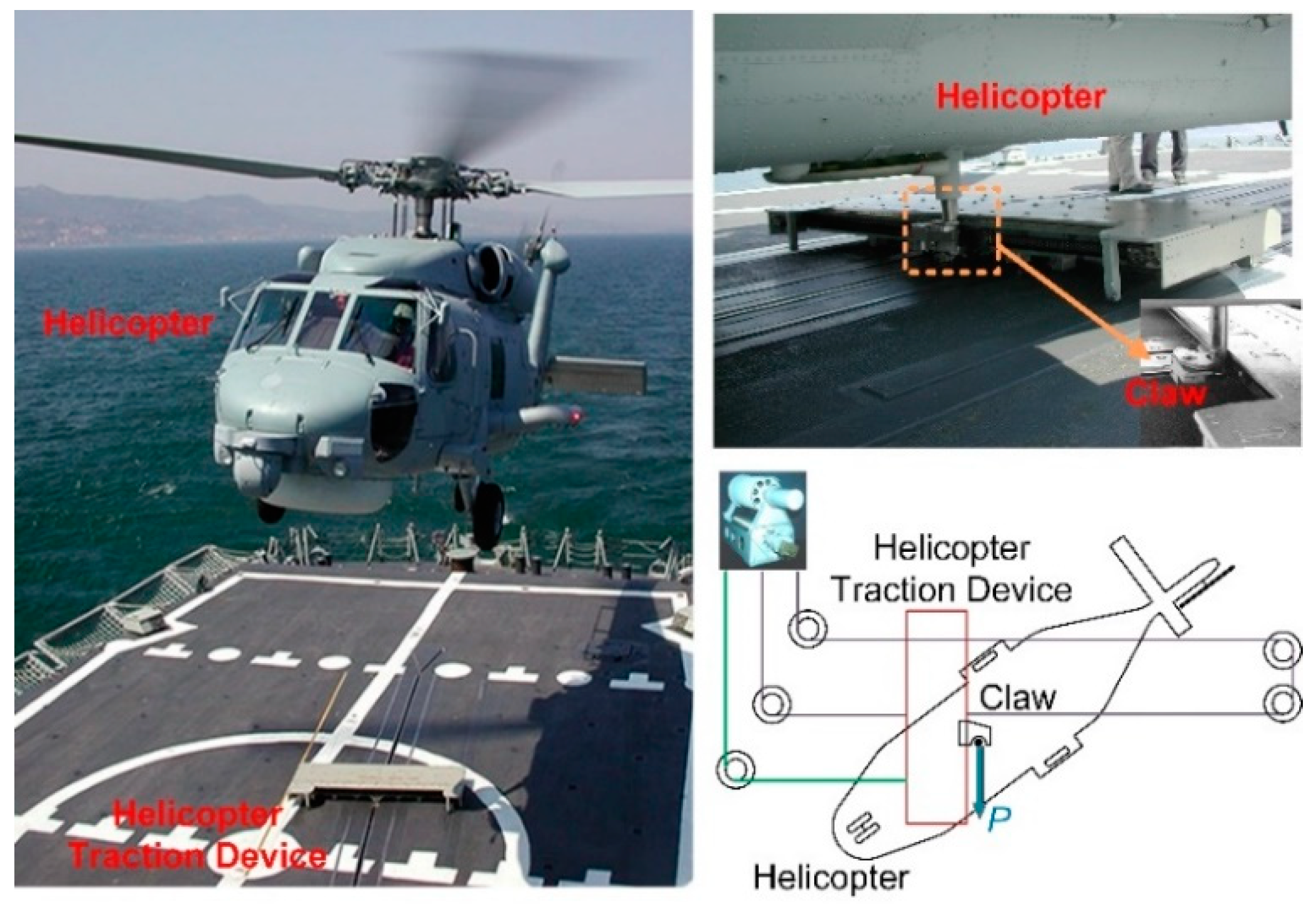
2. Principles of Helicopter Traction Devices

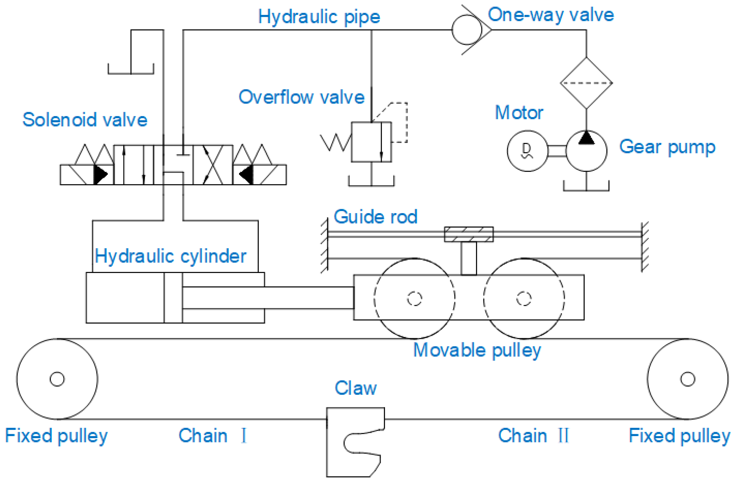
2.1. Transmission Principle of HTD

The working principle of the transmission system of the HTD is shown in Figure 3. The HTD drives the gear pump to output high-pressure hydraulic oil through the motor. Hydraulic oil, in turn, through the hydraulic pipe, one-way valve, and solenoid valve to drive the hydraulic cylinder movement. Finally, the motion of the hydraulic cylinder rod is transformed into the lateral motion of the claw by the pulley-and-chain transmission system. Among them, the movable pulley is also guided by the guide rod in the movement process. The solenoid valve is used to change the movement direction of the claw. The overflow valve is used to limit the maximum pressure of the system, thereby limiting the maximum thrust output of the claw. In Figure 3, the claw is floatable when the solenoid valve is in the middle stage.

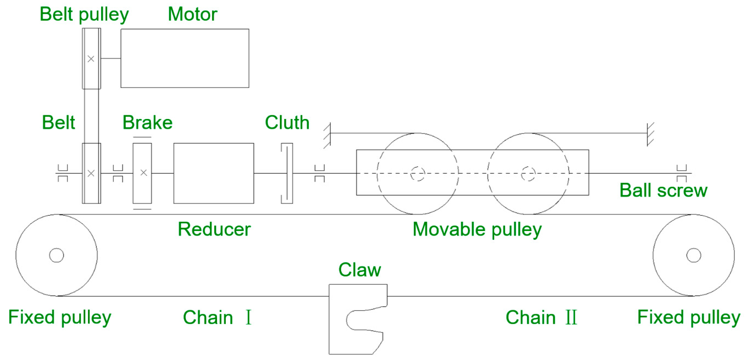
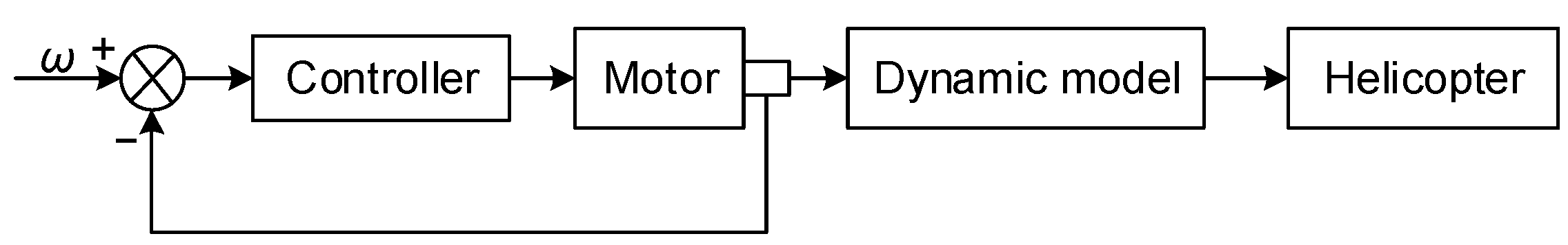
2.2. Transmission Principle of the ETD

The working principle of the transmission system of the ETD is shown in Figure 4. The motor drives the ball screw rotation through the belt pulley, belt, and reducer. Then, the ball nut converts the rotary motion of the ball screw into the linear motion of the movable pulley. Finally, through the pulley-and-chain transmission system, it is transformed into the lateral movement of the claw.

3. System Dynamics Model

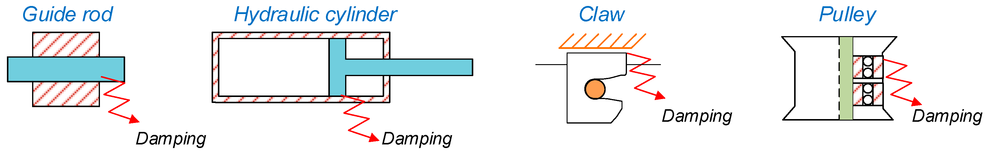
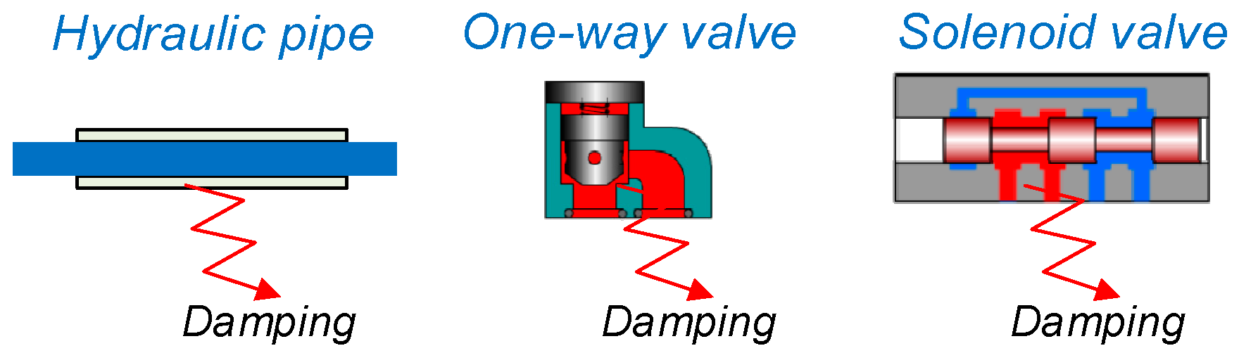
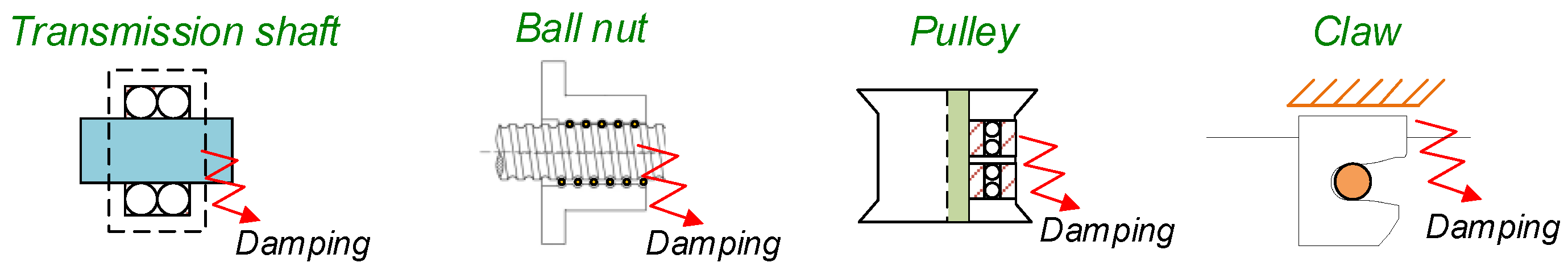
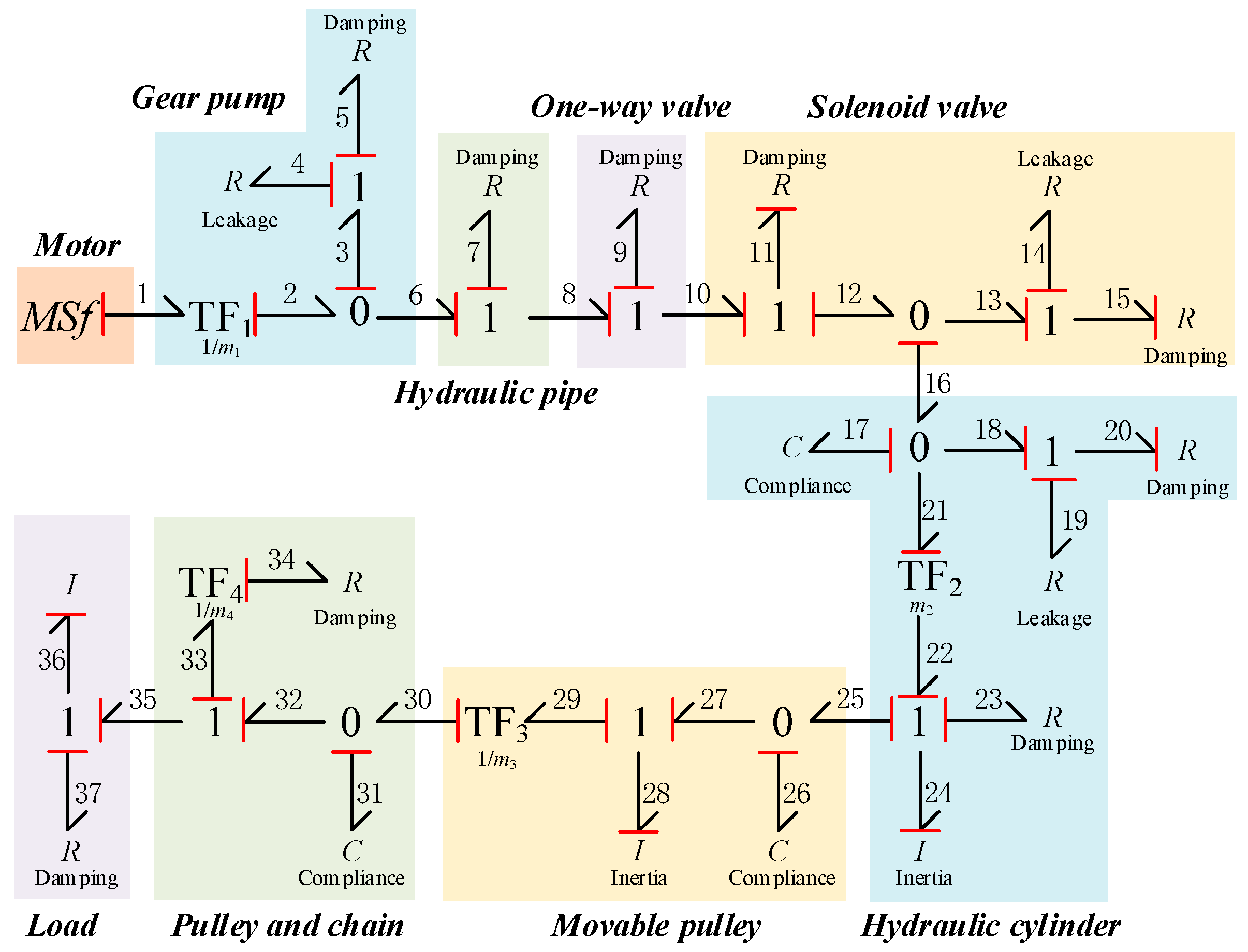
3.1. Energy Consumption Analysis of HTD

For the HTD, the energy loss of the system in the working process mainly includes the following aspects.

• Motion damping

The motion damping of the system includes the friction damping between the claw and the guide rail, the hydraulic cylinder rod and hydraulic cylinder, the movable pulley and guide rod, and the friction damping of the ball bearing installed inside the pulley, as shown in Figure 5.

2.

Flow damping

In the hydraulic system, the flow damping of the hydraulic oil that flows through the pipe, one-way valve, and solenoid valve should also be considered, as shown in Figure 6.

3.

Leakage loss

Internal leakage is inevitable in the working process of the hydraulic system. In the HTD, the internal leakage involved mainly includes the solenoid valve, hydraulic cylinder, and gear pump leakage, as shown in Figure 7.

4.

Energy storage loss

In addition to the direct energy loss mentioned above, energy storage loss occurs during the system acceleration stage, including inertial and capacitive energy storage.

The inertial energy storage includes the kinetic energy stored by the hydraulic cylinder and movable pulley, as shown in Figure 8. The capacitance energy storage includes the elastic potential energy stored by the hydraulic oil and the deformation of the chain and movable pulley shaft under stress, as shown in Figure 9.

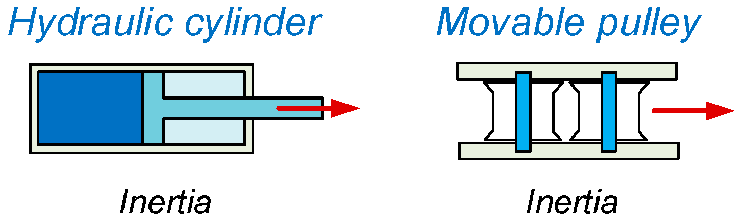
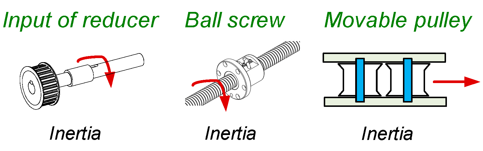
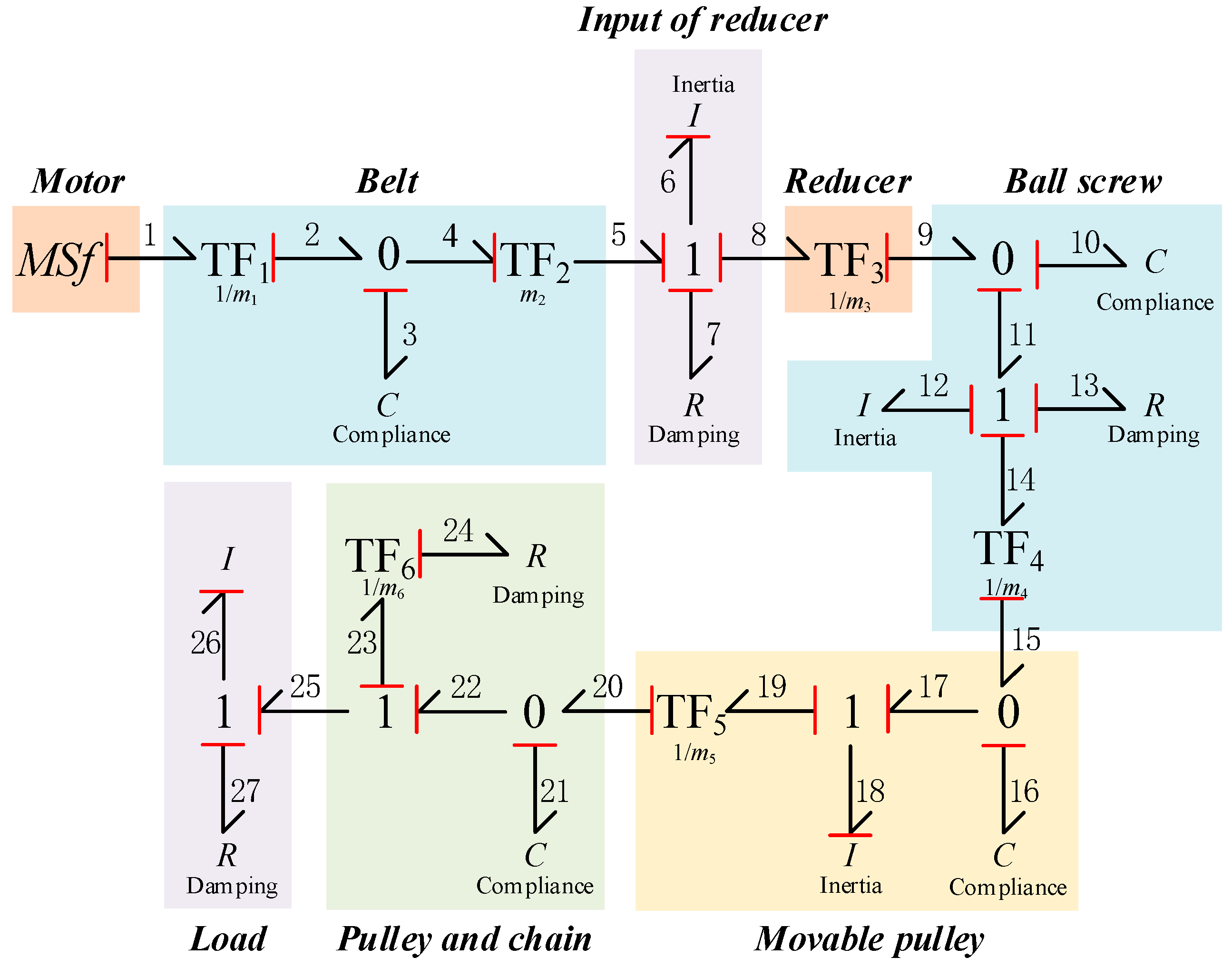
3.2. Energy Consumption Analysis of the ETD

For the ETD, the energy loss of the system in the working process is free of flow damping and leakage loss, mainly including movement damping and energy storage loss.

• Motion damping

The motion damping of the ETD in the working process mainly includes the rotational damping of the transmission shaft, ball nut, pulley, and friction damping of the claw, as shown in Figure 10.

2.

Energy storage loss

In the ETD, the inertial energy storage includes the kinetic energy stored at the input of the reducer, ball screw, and movable pulley, as shown in Figure 11. The capacitance energy storage consists of the elastic potential energy stored due to the deformation of the belt, ball screw, chain, and movable pulley shaft under stress, as shown in Figure 12.

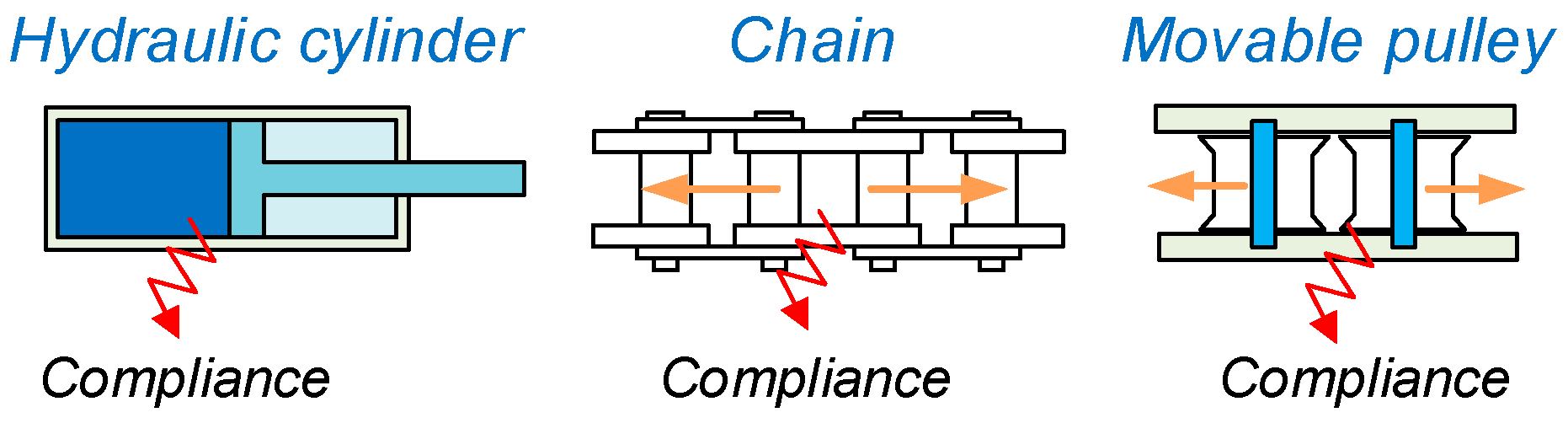
3.3. System Dynamics Model

According to the basic principle of energy conservation, the essential elements in the system are represented by prescribed symbols and connected in series according to specific connection ways to form the system bond graph. The bond graph is a visual representation of the dynamic performance of the components in the system. In order to integrate the state equations of components in different energy domains more easily and intuitively, the bond-graph theory unifies a variety of physical parameters into four generalized variables, namely potential variable e, flow variable f, generalized momentum p, and generalized displacement q. The corresponding relationship of the above four generalized variables in the energy domain of mechanical and hydraulic is shown in

Table 1. The physical meaning of the four generalized variables.

Driving Part	Translational Motion		Rotation Motion		Liquid Flow
	Value	Unit	Value	Unit	Value	Unit
Potential variable	Force	N	Torque	N·m	Pressure	N/m2
Flow variable	Velocity	m/s	Angular velocity	rad/s	Flow	m3/s
Generalized momentum	Momentum	N·s	Angular momentum	N·m·s	Pressure momentum	(N·s)/m2
Generalized displacement	Displacement	m	Angular displacement	rad	Volume	m3

.

Although the bond-graph model is drawn according to the flow of system power transfer, in the current research, the bond graph is mainly used to construct the state equation of the system and analyze its dynamic characteristics. Still, almost no one has used it for the energy consumption analysis of the system. It is easy to notice that, in the process of building a bond-graph model, the information transmitted by each bond includes potential variable e and flow variable f. That is, the energy transmitted by each bond is

$$E(t)={\displaystyle {\int }_0^{t}e(t)f(t)dt}$$

(1)

It should be noted that the bond-graph theory simplifies many nonlinear variables to simplify the mathematical model and state equation of the system. For example, flow damping and motion damping are reduced to linear functions of velocity, and internal leakage of oil is reduced to linear functions of pressure. This way of modeling makes the bond-graph model a linear time-invariant system. However, this does not prevent it from being used for energy analysis in this paper because the engineer expects the trend or percentage of energy consumption, which helps optimize the system model during the design phase.

• Resistance element

The internal motion damping of the system, including friction damping and flow damping, is represented by the symbol R. The characteristic equation and energy consumption equation of the element are as follows

$$\{\begin{array}{l}e(t)=Rf(t)\\ E(t)={\displaystyle {\int }_0^{t}e(t)f(t)dt}={\displaystyle {\int }_0^{t}R{f}^2(t)dt}\end{array}$$

(2)

It is worth noting that, for the convenience of description, the oil leakage in the hydraulic system is often represented by the resistance element R, whose characteristic equation and energy consumption equation are as follows

$$\{\begin{array}{l}f(t)=Re(t)\\ E(t)={\displaystyle {\int }_0^{t}e(t)f(t)dt}={\displaystyle {\int }_0^{t}R{e}^2(t)dt}\end{array}$$

(3)

2.

Compliance element

The elastic potential energy stored in the system is represented by the compliance element, including the compression of the hydraulic oil and the deformation of the chain, belt, etc., denoted by the symbol C. The characteristic equation and energy consumption equation of the element are as follows

$$\{\begin{array}{l}e(t)=\frac{q(t)}{C}\\ E(t)={\displaystyle {\int }_0^{t}e(t)f(t)dt}=={\displaystyle {\int }_0^t\frac{q(t)}{C}f(t)dt}\end{array}$$

(4)

3.

Inertance element

The inertance elements describe the kinetic energy stored in the system, represented by I. The characteristic equation and energy consumption equation of the element are as follows

$$\{\begin{array}{l}f(t)=\frac{p(t)}{I}\\ E(t)={\displaystyle {\int }_0^{t}e(t)f(t)dt}={\displaystyle {\int }_0^{t}e(t)\frac{p(t)}{I}dt}\end{array}$$

(5)

4.

Auxiliary element

The power bond-graph theory also includes three auxiliary elements, namely the energy source, converter, and connector, to represent the system model more intuitively and effectively.

The output speed of the motor is regarded as the energy source, which is represented by Sf.

The converter is mainly used to describe the transmission characteristics of the hydraulic cylinder, ball screw, etc., expressed by the symbol TF, and its characteristic equation is

$$\{\begin{array}{l}{e}_b=m{e}_a\\ f_a=m{f}_b\end{array}$$

(6)

The connector includes a 0-junction and 1-junction. The 0-junction is used to connect the input or output ports with the same potential variables, and the 1-junction is used to connect input or output ports with the same flow variables. Their respective characteristic equations are

$$\{\begin{array}{l}{e}_1=e_2=\dots =e_n\\ {\displaystyle \sum _{i=1}^n{\alpha }_i{f}_i=0}\end{array}$$

(7)

$$\{\begin{array}{l}{f}_1=f_2=\dots =f_n\\ {\displaystyle \sum _{i=1}^n{\alpha }_i{e}_i=0}\end{array}$$

(8)

where α_i = 1 for the energy inflow and α_i = −1 for the energy outflow.

Then, according to this energy transfer property of the bond graph, we can obtain the following lemmas:

Lemma 1.

In the process of system energy transfer, the energy consumption caused by resistance elements is

$$E_R\left(t\right)={\displaystyle {\int }_0^t\left[{\displaystyle \sum _i{R}_i{e}_i^2}\right]dt}$$

(9)

In particular, the leakage effect of the hydraulic system is

$$E_R\left(t\right)={\displaystyle {\int }_0^t\left[{\displaystyle \sum _i{R}_i{f}_i^2}\right]dt}$$

(10)

Lemma 2.

In the process of system energy transfer, the energy consumption caused by compliance elements is

$$E_C\left(t\right)={\displaystyle {\int }_0^t\left({\displaystyle \sum _j\frac{q_j}{C_j}{f}_j}\right)dt}$$

(11)

Lemma 3.

In the process of system energy transfer, the energy consumption caused by inertance elements is

$$E_I\left(t\right)={\displaystyle {\int }_0^t\left({\displaystyle \sum _k\frac{p_k}{I_k}{e}_k}\right)dt}$$

(12)

where, i, j, and k are the symbol subscripts of R, C, and I in the bond graph, respectively.

The power bond-graph model of the HTD can be established according to the above description of the energy transfer process and the energy consumption link, as shown in Figure 13. The generalized displacement q₁₇, q₂₆, and q₃₁ of the compliance elements and the generalized momentum p₂₄, p₂₈, and p₃₆ of the inertance elements are taken as the state variables of the HTD. Take the state equation as follows

$${\dot{X}}_1=A_1\cdot X_1+B_1\cdot U_1$$

(13)

where the state variable is shown as follows

$$X_1={\left[\begin{array}{cccccc}{q}_{17}& p_{24}& q_{26}& p_{28}& q_{31}& p_{36}\end{array}\right]}^{\mathrm{T}}$$

(14)

The input of the system is shown as follows

$$U_1=\left[MSf\right]$$

(15)

From Equations (2)–(8), the constant-coefficient matrix A₁ and the control matrix B₁ can be obtained in the following form

$$A_1=\left[\begin{array}{cccccc}-\frac{M}{C_{17}}& -\frac{m_2}{I_{24}}& 0& 0& 0& 0\\ \frac{m_2}{C_{17}}& -\frac{R_{23}}{I_{24}}& -\frac{1}{C_{26}}& 0& 0& 0\\ 0& \frac{1}{I_{24}}& 0& -\frac{1}{I_{28}}& 0& 0\\ 0& 0& \frac{1}{C_{26}}& 0& -\frac{1}{m_3{C}_{31}}& 0\\ 0& 0& 0& \frac{1}{m_3{I}_{28}}& 0& -\frac{1}{I_{36}}\\ 0& 0& 0& 0& \frac{1}{C_{31}}& -\frac{R_{34}+m_4{}^2{R}_{37}}{m_4{}^2{I}_{36}}\end{array}\right]$$

(16)

$$B_1=\left[\begin{array}{c}\frac{1}{m_{1}N}\\ 0\\ 0\\ 0\\ 0\\ 0\end{array}\right]$$

(17)

where

$$\begin{gathered} N=1+R_4\left(R_7+R_9+R_{11}\right)/\left(1+R_4{R}_5\right), \\ M=R_4/\left[N\left(1+R_4{R}_5\right)\right]+R_{14}/\left(1+R_{14}{R}_{15}\right)+R_{19}/\left(1+R_{19}{R}_{20}\right) \end{gathered}$$

The system input energy is the motor output energy. The useful energy of the system includes the kinetic energy stored by the load and the energy consumed by the damping of the load. The energy equations for the system are as follows

$$E_{in}\left(t\right)={\displaystyle {\int }_0^t{P}_{in}dt}={\displaystyle {\int }_0^t{e}_{1}MSfdt}$$

(18)

$$E_{out}\left(t\right)={\displaystyle {\int }_0^t{P}_{out}dt}={\displaystyle {\int }_0^t\left[e_{36}\frac{p_{36}}{I_{36}}+R_{37}{\left(\frac{p_{36}}{I_{36}}\right)}^2\right]dt}$$

(19)

The energy consumed by resistance elements includes

$$E_{R1}\left(t\right)={\displaystyle {\int }_0^t\left[R_4{e}_4^2+R_{14}{e}_{14}^2+R_{19}{e}_{19}^2\right]dt}$$

(20)

$$E_{R2}\left(t\right)={\displaystyle {\int }_0^t\left[\left(R_7+R_9+R_{11}\right)f_6^2+R_{15}{f}_{15}^2+R_{20}{f}_{20}^2+R_{23}{f}_{23}^2+R_{34}{f}_{34}^2\right]dt}$$

(21)

The energy consumed by compliance elements includes

$$E_C\left(t\right)={\displaystyle {\int }_0^t\left(\frac{q_{17}}{C_{17}}{f}_{17}+\frac{q_{26}}{C_{26}}{f}_{26}+\frac{q_{31}}{C_{31}}{f}_{31}\right)dt}$$

(22)

The energy consumed by inertance elements includes

$$E_I\left(t\right)={\displaystyle {\int }_0^t\left(\frac{p_{24}}{I_{24}}{e}_{24}+\frac{p_{28}}{I_{28}}{e}_{28}\right)dt}$$

(23)

The power bond-graph model of the ETD is shown in Figure 14. The generalized displacement q₃, q₁₀, q₁₆, and q₂₁ of the compliance elements and the generalized momentum p₆, p₁₂, p₁₈, and p₂₆ of the inertance elements are taken as the state variables of the ETD, and the state equation and energy equation of the system can be obtained as follows

$${\dot{X}}_2=A_2\cdot X_2+B_2\cdot U_2$$

(24)

where the state variable is shown as follows

$$X_2={\left[\begin{array}{cccccccc}{q}_3& p_6& q_{10}& p_{12}& q_{16}& p_{18}& q_{21}& p_{26}\end{array}\right]}^{\mathrm{T}}$$

(25)

The input of the system is shown as follows

$$U_2=\left[MSf\right]$$

(26)

The constant-coefficient matrix A₁ and the control matrix B₁ can be obtained in the following form

$$A_2=\left[\begin{array}{cccccccc}0& -\frac{m_2}{I_6}& 0& 0& 0& 0& 0& 0\\ \frac{m_2}{C_3}& -\frac{R_7}{I_6}& -\frac{1}{m_3{C}_{10}}& 0& 0& 0& 0& 0\\ 0& \frac{1}{m_3{I}_6}& 0& -\frac{1}{I_{12}}& 0& 0& 0& 0\\ 0& 0& \frac{1}{C_{10}}& -\frac{R_{13}}{I_{12}}& -\frac{1}{m_4{C}_{16}}& 0& 0& 0\\ 0& 0& 0& \frac{1}{m_4{I}_{12}}& 0& -\frac{1}{I_{18}}& 0& 0\\ 0& 0& 0& 0& \frac{1}{C_{16}}& 0& -\frac{1}{m_5{C}_{21}}& 0\\ 0& 0& 0& 0& 0& \frac{1}{m_5{I}_{18}}& 0& -\frac{1}{I_{26}}\\ 0& 0& 0& 0& 0& 0& \frac{1}{C_{21}}& -\frac{R_{24}+m_6{}^2{R}_{27}}{m_6{}^2{I}_{26}}\end{array}\right]$$

(27)

$$B_2=\left[\begin{array}{c}\frac{1}{m_1}\\ 0\\ 0\\ 0\\ 0\\ 0\\ 0\\ 0\end{array}\right]$$

(28)

The energy equation of the system can be obtained as follows

$$E_{in}\left(t\right)={\displaystyle {\int }_0^t\frac{q_{3}MSf}{m_1{C}_3}dt}$$

(29)

$$E_{out}\left(t\right)={\displaystyle {\int }_0^t\left[e_{26}\frac{p_{26}}{I_{26}}+R_{27}{\left(\frac{p_{26}}{I_{26}}\right)}^2\right]dt}$$

(30)

$$E_R\left(t\right)={\displaystyle {\int }_0^t\left[R_7{f}_7^2+R_{13}{f}_{13}^2+R_{24}{f}_{24}^2\right]dt}$$

(31)

$$E_C\left(t\right)={\displaystyle {\int }_0^t\left(\frac{q_3}{C_3}{f}_3+\frac{q_{10}}{C_{10}}{f}_{10}+\frac{q_{16}}{C_{16}}{f}_{16}+\frac{q_{21}}{C_{21}}{f}_{21}\right)dt}$$

(32)

$$E_I\left(t\right)={\displaystyle {\int }_0^t\left(\frac{p_6}{I_6}{e}_6+\frac{p_{12}}{I_{12}}{e}_{12}+\frac{p_{18}}{I_{18}}{e}_{18}\right)dt}$$

(33)

4. Simulation Tests

4.1. The Simulation Conditions

A simulation model was built, and simulation tests were carried out, according to Figure 15. The simulation time was selected as 2 s; the claw speed was 0.01 m/s according to the actual use requirements of the helicopter traction device. The motor controller used in the simulation is a PID controller based on torque control [38,39]. The system parameters used in the simulation are shown in

Table 2. The system parameters of HTD.

Driving Part	Symbol	Value	Unit
Gear pump	TF1	3.14 × 106	rad/m3
	R4	3.21 × 10−12	m3/(s·pa)
	R5	4.72 × 105	pa·s/m3
Hydraulic pipe	R7	1.81 × 108	pa·s/m3
One-way valve	R9	8.76 × 109	pa·s/m3
Solenoid valve	R11	1.03 × 1010	pa·s/m3
	R14	3.3 × 10−13	m3/(s·pa)
	R15	1.32 × 104	pa·s/m3
Hydraulic cylinder	C17	2.51 × 10−14	m3/pa
	R19	1.04 × 10−12	m3/(s·pa)
	R20	6.37 × 106	pa·s/m3
	TF2	5.02 × 10−3	m2/s
	I24	46.32	kg
	R23	60.0	N
Movable pulley	I28	35.75	kg
	TF3	0.5
	C26	4.3 × 10−9	m/N
Pulley and chain	C31	1.49 × 10−8	m/N
	R34	7.6 × 10−2	N·m·s
	TF4	56.25 × 10−3	m/rad
Load	R37	1 × 104	N
	I36	6.04 × 103	kg

and

Table 3. The system parameters of ETD.

Driving part	Symbol	Value	Unit
Belt	TF1	20.61	rad/m
	C3	1.92 × 10−7	m/N
	TF2	48.52 × 10−3	m/rad
Input of reducer	I6	4.25 × 10−3	kg·m2
	R7	7.6 × 10−4	N·m·s
Reducer	TF3	40	--
Ball screw	C10	7.8 × 10−6	rad/(N·m)
	I12	22.95 × 10−3	kg·m2
	R13	7.3 × 10−4	N·m·s
	TF4	628.93	Rad/m
Movable pulley	I18	35.75	kg
	TF5	0.5
	C16	4.3 × 10−9	m/N
Pulley and chain	C21	1.49 × 10−9	m/N
	R24	7.6 × 10−2	N·m·s
	TF6	56.25 × 10−3	m/rad
Load	R27	1 × 104	N
	I26	6.04 × 103	kg

.

The motor model based on torque control is shown in Figure 16 to describe the state of the system accurately, and the characteristic equation is

$$MSf={\displaystyle \int \frac{T}{J}}dt$$

(34)

where T is the output torque of the motor and J is the moment of inertia of the motor rotor.

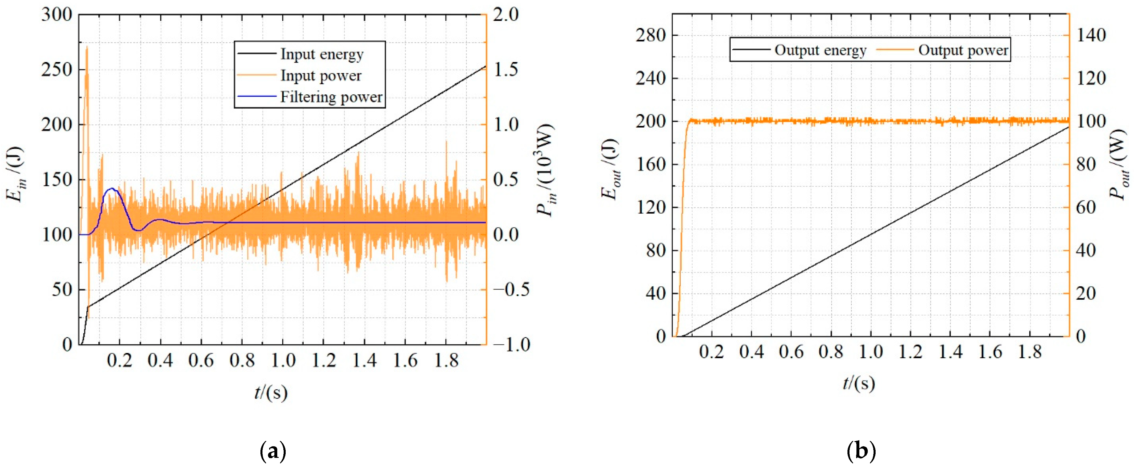
4.2. Dynamic Characteristics and Energy Consumption Characteristics of HTD

When the speed of the traction helicopter was set at 0.01 m/s, the simulated motor output speed and torque curve are shown in Figure 17a, and the motion speed curve of the helicopter is shown in Figure 17b.

As shown in Figure 17a, the output speed and torque of the motor increase rapidly from 0s, and reach a steady state at about 0.08 s~0.1 s. At this time, the output speed of the motor is about 140 rad/s, and the output torque is about 1.45 N·m. As shown in Figure 17b, the load reaches a steady state at about 0.08 s~0.1 s and mov at a uniform speed.

The energy curve and power curve of the system input are shown in Figure 18a, and the energy curve and power curve of system output are shown in Figure 18b.

As shown in Figure 18a, the total energy input by the motor of HTD was about 395 J after working for 2s, and the stable state input power was about 202 W. It can be seen from Figure 18b that the system output energy was about 193 J, and the steady-state output power fluctuated around 99 W.

In addition, the energy and power curves consumed by the resistance elements and energy storage elements in the transmission process of HTD are shown in Figure 19.

It can be seen from Figure 19a that the energy consumed by the resistance elements of the system increases sharply from 0 s. When the system reaches a steady state at about 0.08 s~1 s, the power of the resistance elements begins to stabilize, and the energy consumed by the resistance elements increases linearly. The energy consumed by the resistance elements is about 201 J in 2 s, and the steady-state power fluctuates around 103 W.

As shown in Figure 19b, different from the energy consumption of the resistance elements, the energy consumption of the energy storage elements of the system is only about 1.14 J within 2 s. It can be seen from the power variation curve that the energy consumed by the energy storage elements mainly occurs in the system acceleration stage. When the system enters the steady state, the energy storage elements are saturated and no longer consume energy.

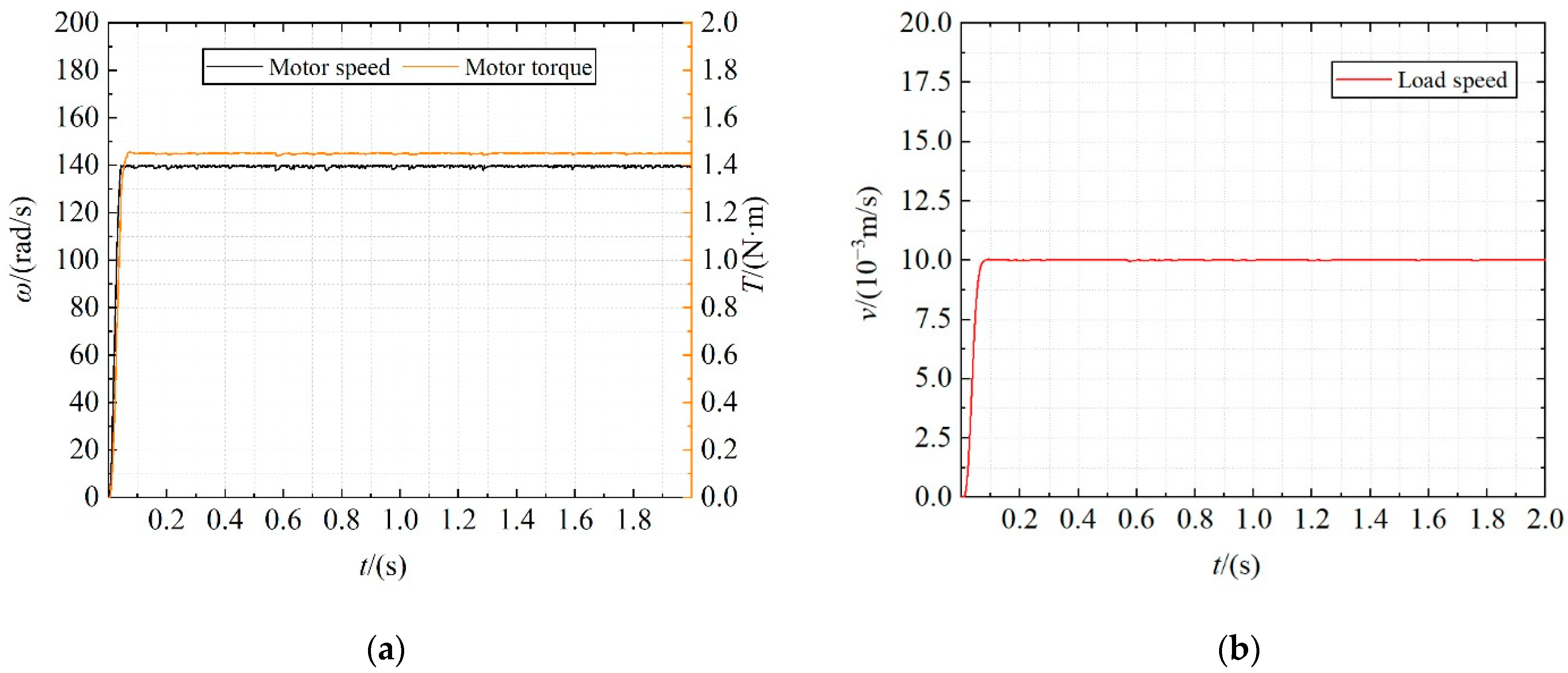
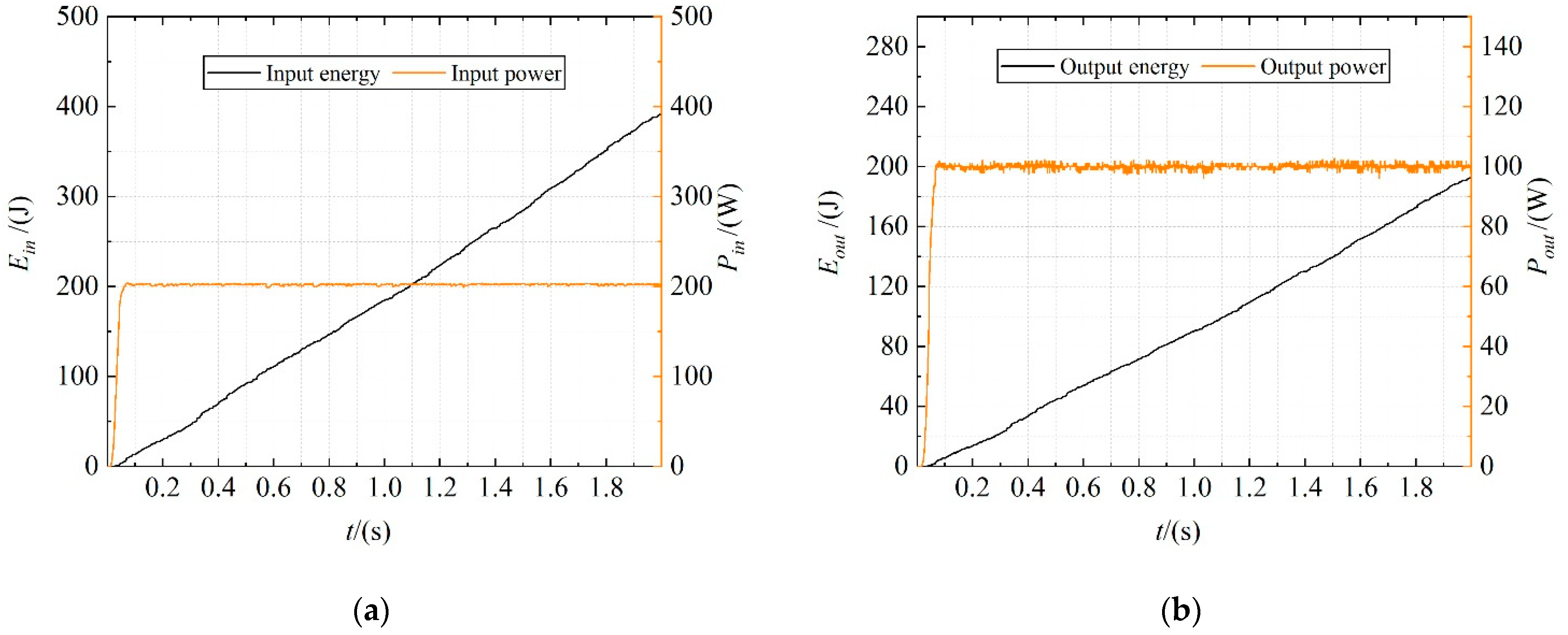
4.3. Dynamic Characteristics and Energy Consumption Characteristics of the ETD

Similarly, for the ETD, when the traction speed is set at 0.01 m/s, the simulated motor output speed and torque curve are shown in Figure 20a, and the helicopter speed curve is shown in Figure 20b. The steady-state errors of the HTD and ETD are shown in Figure 21.

As shown in Figure 20a, the motor output speed reaches a steady state at about 0.05 s, at which the speed is 126 rsd/s. The motor torque increases sharply in the acceleration stage and fluctuates sharply in the steady-state phase. This phenomenon is because the ETD, compared with the HTD, reduces most of the transmission parts, making the motor end load more sensitive to changes in system characteristics. After filtering, the steady output torque of the motor is about 1.25 N·m. Correspondingly, as shown in Figure 20b, the speed change of load in the steady state is more stable, which is also caused by the sensitive adaptation of motor output torque.

As shown in Figure 21, compared with the HTD, the ETD can achieve higher control accuracy in a steady state because the output torque of the motor can accurately reflect the dynamic characteristics of the system.

The energy curve and power curve of system input are shown in Figure 22a, and the energy curve and power curve of system output are shown in Figure 22b.

As shown in Figure 22a, after the ETD works for 2 s, the system input energy is about 254 J, while the input power fluctuates violently, corresponding to Figure 20a. After filtering, the steady-state input power is about 112.5 W. Figure 22b shows that the output energy is about 195 J, and the steady-state output power fluctuates around 100 W.

In addition, the energy and power curves consumed by the resistance elements and energy storage elements in the transmission process of the ETD are shown in Figure 23.

It can be seen from Figure 23a that the energy consumed by the resistance elements of the system also increases sharply from 0 s. When the system reaches a steady state at 0.05 s, the power of the resistance elements begins to stabilize, and the energy consumed by the resistance elements begins to increase linearly. The energy consumed by the resistance elements of the ETD is about 24 J, and the steady-state power fluctuates around 12 W, which is much lower than the HTD.

As shown in Figure 23b, the energy consumed by the energy storage elements mainly occurs in the acceleration stage of the system. When the system enters the steady state, the energy storage elements are saturated and no longer consume energy. However, the energy consumption of energy storage elements is much higher than the HTD, which is as high as 35 J within 2 s.

In addition, it can be seen from Figure 20, 22, and 23 that the input torque and input power of the ETD fluctuate significantly because of the fluctuation of the energy storage element. On the one hand, the ETD is more sensitive to the representation of the dynamic characteristics of the system. On the other hand, the motor control system can adjust the output torque in real-time according to the motor speed feedback, which leads to the speed fluctuation of the energy storage elements.

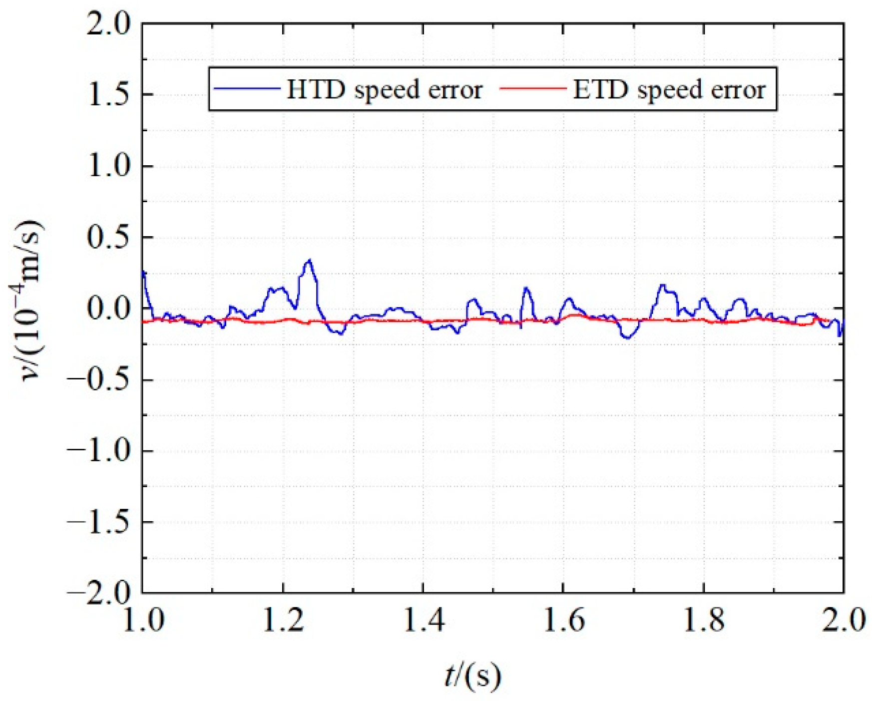
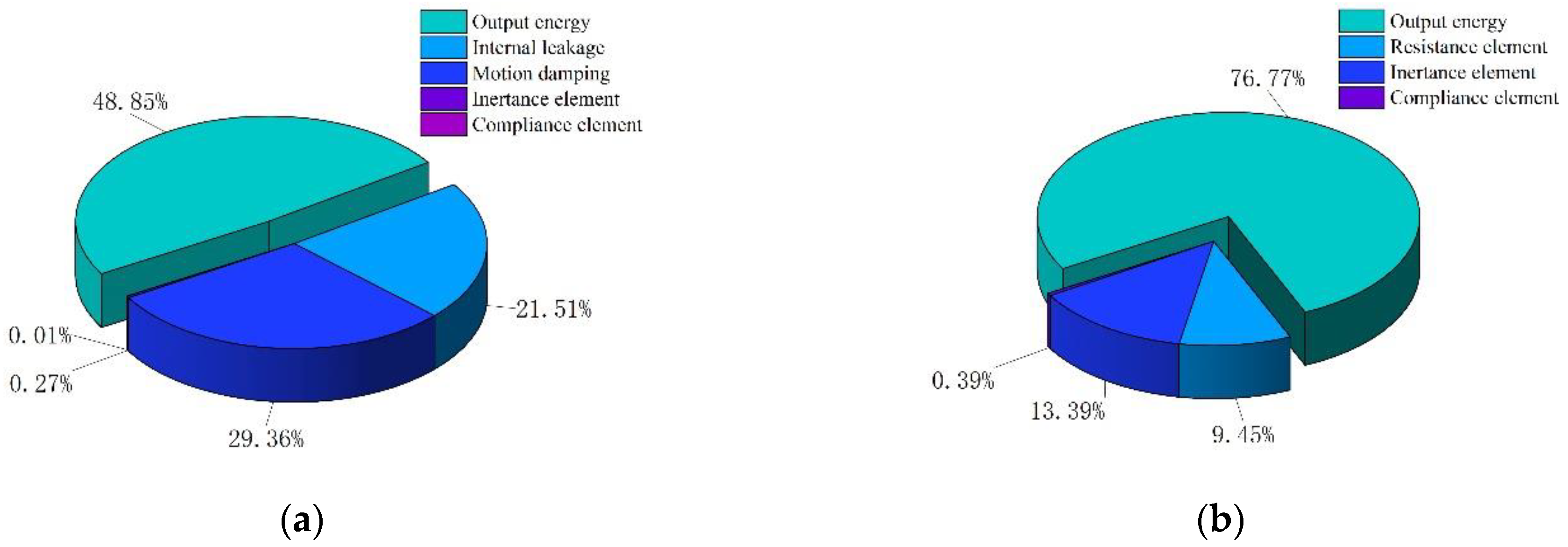
4.4. Analysis of Energy Consumption

For the HTD, the energy utilization rate within 2 s can be obtained from Equation (35), and the calculated energy utilization rate is about 48.85%. In the steady state, the energy transfer efficiency of the system can be obtained from Equation (36), and the calculated transfer efficiency in the steady state is about 49%.

$${\eta }_1=\frac{E_{in}}{E_{out}}$$

(35)

$${\eta }_2=\frac{P_{in}}{P_{out}}$$

(36)

After ETD works for 2 s, the energy utilization rate is 76.77%, and the energy transfer efficiency of the system is about 88.89% in the steady state.

Figure 24 shows the energy consumption ratio of the HTD and ETD. The energy consumption of the energy storage elements is further divided into inertance elements and compliance elements to describe this characteristic more accurately. The resistance elements in the HTD are divided into internal leakage and motion damping.

As shown in Figure 24, the energy consumption loss of the HTD is more concentrated on the resistance elements, accounting for about 50.87%. Among them, the resistance loss accounted for 29.36% of the total energy consumption of the system, and the leakage loss accounted for 21.51%. On the contrary, the energy loss of the ETD is more concentrated in the energy storage elements, accounting for about 14%, among which the energy storage loss caused by the inertance elements is as high as 13.39%.

This phenomenon is expected for the high-pressure, high-flow hydraulic system used in the HTD. Relatively high pressure and flow will inevitably lead to severe system leakage and resistance loss. As for the ETD, the energy storage loss caused by the inertance elements is mainly caused by the high speed and large inertia transmission parts at the input end of the reducer.

5. Conclusions

Based on the power bon-graph theory, this paper proposes a modeling method that takes into account the dynamic characteristics and energy consumption characteristics of the system and brings the helicopter traction device as an example for analysis and simulation test. The following conclusions can be drawn from the simulation results.

• The proposed modeling method can better reflect the dynamic characteristics of the system and accurately describe the energy consumption trend in each link of the system. This modeling method is mainly used for energy consumption analysis and the optimization design of shipborne equipment. It also has essential reference significance for the modeling and analysis of other complex mechanical systems.
• Compared with the HTD, the ETD has a higher energy utilization rate and more stable system operation in the steady state. Therefore, in shipborne equipment, it is of great significance to popularize the application of electric drive equipment to improve the capability of ocean voyages and long-term combat.
• The energy consumption of the HTD is mainly concentrated on the resistance elements, accounting for 50.87% of the total energy consumption. The energy consumption of the ETD is mainly concentrated in the inertance elements, accounting for 13.39% of the total energy consumption. This conclusion is helpful for designers to optimize the energy consumption of the system and improve its efficiency.

References

1. Beecher, J.D. The FFG7 guided missle frigate program model for the future. Nav. Eng. J. 1978, 90, 93–105. [Google Scholar] [CrossRef]
2. Hu, Z.; Jin, Y.; Hu, Q.; Sen, S.; Zhou, T.; Osman, M.T. Prediction of Fuel Consumption for Enroute Ship Based on Machine Learning. IEEE Access 2019, 7, 119497–119505. [Google Scholar] [CrossRef]
3. Yu, H.; Fang, Z.; Fu, X.; Liu, J.; Chen, J. Literature review on emission control-based ship voyage optimization. Transp. Res. Part D Transp. Environ. 2021, 93, 102768. [Google Scholar] [CrossRef]
4. Man, Y.; Sturm, T.; Lundh, M.; MacKinnon, S.N. From Ethnographic Research to Big Data Analytics—A Case of Maritime Energy-Efficiency Optimization. Appl. Sci. 2020, 10, 2134. [Google Scholar] [CrossRef] [Green Version]
5. Balsamo, F.; De Falco, P.; Mottola, F.; Pagano, M. Power Flow Approach for Modeling Shipboard Power System in Presence of Energy Storage and Energy Management Systems. IEEE Trans. Energy Convers. 2020, 35, 1944–1953. [Google Scholar] [CrossRef]
6. Nuchturee, C.; Li, T.; Xia, H. Energy efficiency of integrated electric propulsion for ships—A review. Renew. Sustain. Energy Rev. 2020, 134, 110145. [Google Scholar] [CrossRef]
7. Taymourtash, N.; Zagaglia, D.; Zanotti, A.; Muscarello, V.; Gibertini, G.; Quaranta, G. Experimental study of a helicopter model in shipboard operations. Aerosp. Sci. Technol. 2021, 115, 106774. [Google Scholar] [CrossRef]
8. Zhang, Z.; Liu, Q.; Zhao, D.; Wang, L.; Yang, P. Research on Shipborne Helicopter Electric Rapid Secure Device: System Design, Modeling, and Simulation. Sensors 2022, 22, 1514. [Google Scholar] [CrossRef]
9. Zhang, Z.; Liu, Q.; Zhao, D.; Wang, L.; Jia, T. Electrical Aircraft Ship Integrated Secure and Traverse System Design and Key Characteristics Analysis. Appl. Sci. 2022, 12, 2603. [Google Scholar] [CrossRef]
10. Wang, Q.; Zhao, D.X.; Wei, H.L.; Zhao, Y. Study of the Landing Dynamics of Carrier Based Helicopter Under Complex Sea Conditions. J. Northeast. Univ. (Nat. Sci.) 2017, 38, 1595. [Google Scholar]
11. Zhao, D.X.; Wang, Q.; Zhang, Z.X. Extenics theory for reliability assessment of carrier helicopter based on analytic hierarchy process. J. Jilin Univ. (Eng. Technol. Ed.) 2016, 46, 1528–1531. [Google Scholar]
12. Su, D.; Xu, G.; Huang, S.; Shi, Y. Numerical investigation of rotor loads of a shipborne coaxial-rotor helicopter during a vertical landing based on moving overset mesh method. Eng. Appl. Comput. Fluid Mech. 2019, 13, 309–326. [Google Scholar] [CrossRef]
13. Linn, D.R.; Langlois, R.G. Development and experimental validation of a shipboard helicopter on-deck maneuvering simulation. J. Aircr. 2006, 43, 895–906. [Google Scholar] [CrossRef]
14. Feldman, A.R.; Langlois, R.G. Autonomous straightening and traversing of shipboard helicopters. J. Field Robot. 2006, 23, 123–139. [Google Scholar] [CrossRef]
15. Karpenko, M.; Prentkovskis, O.; Šukevičius, Š. Research on high-pressure hose with repairing fitting and influence on energy parameter of the hydraulic drive. Eksploatacja Niezawodność 2022, 24, 25–32. [Google Scholar] [CrossRef]
16. Karpenko, M.; Bogdevičius, M. Investigation into the hydrodynamic processes of fitting connections for determining pressure losses of transport hydraulic drive. Transport 2020, 35, 108–120. [Google Scholar] [CrossRef] [Green Version]
17. Liu, W.; Li, L.; Cai, W.; Li, C.; Li, L.; Chen, X.; Sutherland, J.W. Dynamic characteristics and energy consumption modelling of machine tools based on bond graph theory. Energy 2020, 212, 118767. [Google Scholar] [CrossRef]
18. Chen, Y.; Sun, Q.; Guo, Q.; Gong, Y. Dynamic Modeling and Experimental Validation of a Water Hydraulic Soft Manipulator Based on an Improved Newton—Euler Iterative Method. Micromachines 2022, 13, 130. [Google Scholar] [CrossRef]
19. Zhang, F.; Yuan, Z. The Study of Coupling Dynamics Modeling and Characteristic Analysis for Flexible Robots with Nonlinear and Frictional Joints. Arab. J. Sci. Eng. 2022, 1–17. [Google Scholar] [CrossRef]
20. Ungureanu, L.M.; Petrescu, F.I.T. Dynamics of Mechanisms with Superior Couplings. Appl. Sci. 2021, 11, 8207. [Google Scholar] [CrossRef]
21. Burghardt, A.; Skwarek, W. Modeling the Dynamics of Two Cooperating Robots. Appl. Sci. 2021, 11, 6019. [Google Scholar] [CrossRef]
22. Burghardt, A.; Gierlak, P.; Skwarek, W. Modeling of dynamics of cooperating wheeled mobile robots. J. Theor. Appl. Mech. 2021, 59, 649–659. [Google Scholar] [CrossRef]
23. Tu, T.W. Dynamic modelling of a railway wheelset based on Kane’s method. Int. J. Heavy Veh. Syst. 2020, 27, 202–226. [Google Scholar] [CrossRef]
24. Qi, F.; Chen, B.; Gao, S.; She, S. Dynamic model and control for a cable-driven continuum manipulator used for minimally invasive surgery. Int. J. Med. Robot. Comput. Assist. Surg. 2021, 17, e2234. [Google Scholar] [CrossRef]
25. Somu, N.; M R, G.R.; Ramamritham, K. A hybrid model for building energy consumption forecasting using long short term memory networks. Appl. Energy 2020, 261, 114131. [Google Scholar] [CrossRef]
26. Wang, G.; Ding, L.; Gao, H.; Deng, Z.; Liu, Z.; Yu, H. Minimizing the Energy Consumption for a Hexapod Robot Based on Optimal Force Distribution. IEEE Access 2019, 8, 5393–5406. [Google Scholar] [CrossRef]
27. Liu, E.; Lv, L.; Yi, Y.; Xie, P. Research on the Steady Operation Optimization Model of Natural Gas Pipeline Considering the Combined Operation of Air Coolers and Compressors. IEEE Access 2019, 7, 83251–83265. [Google Scholar] [CrossRef]
28. Saeedi, M.; Moradi, M.; Hosseini, M.; Emamifar, A.; Ghadimi, N. Robust optimization based optimal chiller loading under cooling demand uncertainty. Appl. Therm. Eng. 2018, 148, 1081–1091. [Google Scholar] [CrossRef]
29. Su, S.; Wang, X.; Cao, Y.; Yin, J. An Energy-Efficient Train Operation Approach by Integrating the Metro Timetabling and Eco-Driving. IEEE Trans. Intell. Transp. Syst. 2019, 21, 4252–4268. [Google Scholar] [CrossRef]
30. Fu, Y.; Tian, G.; Fathollahi-Fard, A.M.; Ahmadi, A.; Zhang, C. Stochastic multi-objective modelling and optimization of an energy-conscious distributed permutation flow shop scheduling problem with the total tardiness constraint. J. Clean. Prod. 2019, 226, 515–525. [Google Scholar] [CrossRef]
31. Wang, Y.; Zhao, D.; Wang, L.; Zhang, Z.; Wang, L.; Hu, Y. Dynamic simulation and analysis of the elevating mechanism of a forklift based on a power bond graph. J. Mech. Sci. Technol. 2016, 30, 4043–4048. [Google Scholar] [CrossRef]
32. Deam, K. Understanding Automobile Roll Dynamics and Lateral Load Transfer Through Bond Graphs. Trans. Korean Soc. Automot. Eng. 1998, 6, 34–44. [Google Scholar]
33. Couenne, F.; Jallut, C.; Maschke, B.; Tayakout, M.; Breedveld, P. Structured modeling for processes: A thermodynamical network theory. Comput. Chem. Eng. 2008, 32, 1120–1134. [Google Scholar] [CrossRef]
34. Borutzky, W.; Barnard, B.; Thoma, J.U. Describing bond graph models of hydraulic components in Modelica. Math. Comput. Simul. 2000, 53, 381–387. [Google Scholar] [CrossRef]
35. Fu, J.; Maré, J.-C.; Fu, Y. Incremental Modeling and Simulation of Mechanical Power Transmission for More Electric Aircraft Flight Control Electromechanical Actuation System Application. In Proceedings of the ASME 2016 International Mechanical Engineering Congress and Exposition, Phoenix, AZ, USA, 11–17 November 2016; American Society of Mechanical Engineers: New York, NY, USA, 2016; Volume 50510, p. V001T03A040. [Google Scholar]
36. Badoud, A.E.; Merahi, F.; Bouamama, B.O.; Mekhilef, S. Bond graph modeling, design and experimental validation of a photovoltaic/fuel cell/electrolyzer/battery hybrid power system. Int. J. Hydrogen Energy 2021, 46, 24011–24027. [Google Scholar] [CrossRef]
37. Song, K.; Wang, Y.; An, C.; Xu, H.; Ding, Y. Design and Validation of Energy Management Strategy for Extended-Range Fuel Cell Electric Vehicle Using Bond Graph Method. Energies 2021, 14, 380. [Google Scholar] [CrossRef]
38. Zhang, X.; Hou, B. Double Vectors Model Predictive Torque Control Without Weighting Factor Based on Voltage Tracking Error. IEEE Trans. Power Electron. 2017, 33, 2368–2380. [Google Scholar] [CrossRef]
39. Faiz, J.; Heidari, M.; Sharafi, H. Torque ripple and switching frequency reduction of interior permanent magnet brushless direct current motors using a novel control technique. IET Power Electron. 2019, 12, 3852–3858. [Google Scholar] [CrossRef]
Figure 1. The working environment of helicopter traction device.
Energies 15 07772 g001
Figure 2. The energy transfer process of HTD and ETD.
Energies 15 07772 g002
Figure 3. The transmission system schematic diagram of HTD.
Energies 15 07772 g003
Figure 4. The transmission system schematic diagram of ETD.
Energies 15 07772 g004
Figure 5. Motion damping schematic diagram of the HTD.
Energies 15 07772 g005
Figure 6. Flow damping schematic diagram of the HTD.
Energies 15 07772 g006
Figure 7. Leakage loss schematic diagram of the HTD.
Energies 15 07772 g007
Figure 8. Inertial energy storage schematic diagram of the HTD.
Energies 15 07772 g008
Figure 9. Capacitive energy storage schematic diagram of the HTD.
Energies 15 07772 g009
Figure 10. Motion damping schematic diagram of the ETD.
Energies 15 07772 g010
Figure 11. Inertial energy storage schematic diagram of the ETD.
Energies 15 07772 g011
Figure 12. Capacitive energy storage schematic diagram of the ETD.
Energies 15 07772 g012
Figure 13. The power bond-graph model of HTD.
Energies 15 07772 g013
Figure 14. The power bond graph model of ETD.
Energies 15 07772 g014
Figure 15. Schematic diagram of the simulation model.
Energies 15 07772 g015
Figure 16. Mathematical model of the motor.
Energies 15 07772 g016
Figure 17. (a) The motor speed and torque of HTD; (b) The load speed of HTD.
Energies 15 07772 g017
Figure 18. (a) The input energy and power of HTD; (b) the output energy and power of HTD.
Energies 15 07772 g018
Figure 19. (a) The energy and power curve of the resistance elements; (b) the energy and power curve of the energy storage elements.
Energies 15 07772 g019
Figure 20. (a) The motor speed and torque of ETD; (b) the load speed of ETD.
Energies 15 07772 g020
Figure 21. The steady-state errors of HTD and ETD.
Energies 15 07772 g021
Figure 22. (a) The input energy and power of ETD; (b) The output energy and power of ETD.
Energies 15 07772 g022
Figure 23. (a) The energy and power curve of the resistance elements; (b) The energy and power curve of the energy storage elements.
Energies 15 07772 g023
Figure 24. (a) The energy consumption ratio of HTD; (b) the energy consumption ratio of ETD.
Energies 15 07772 g024