
Impact of Geometry on a Thermal-Energy Storage Finned Tube during the Discharging Process


Abstract
:1. Introduction
- 1.
- By improving the thermal conductivity of the PCM mass;
- 2.
- By increasing the contact area between the exchanger structure and the PCM mass.
2. Mathematical Modelling of Solidification and Melting Processes
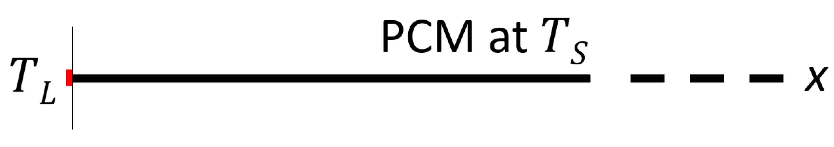
2.1. Analytical Solution of the Classical Two-Phase (One-Dimensional) Stefan Problem
- The heat equation in both the liquid and the solid phases:where is the specific heat and is the thermal conductivity;
- The interface condition:
- The Stefan condition for the one-dimensional case:where represents the values of as ;
- The initial conditions:
- The boundary conditions:
- is the Stefan number:
- ;
- is the error function;
- is the complementary error function.
- Interface location:
- Temperature in the liquid region:
- Temperature in the solid region:
2.2. Matlab Implementation of the Analytical Model
3. Numerical Simulation for the 1-D Problem
3.1. Solidification and Melting Model in Ansys Fluent
- if ;
- if ;
- if .
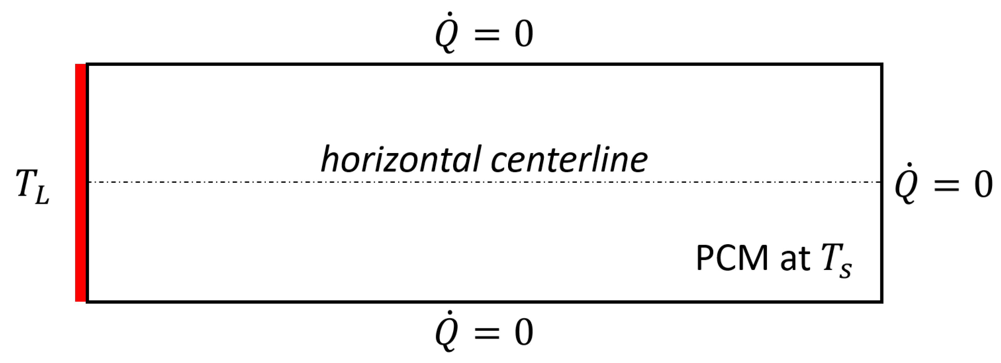
3.2. Numerical Simulation of the Two-Phase 1-D Stefan Problem
- In General, the solver was set to time-transient and 2D-planar analyses. The gravity contribution was not considered;
- In Models the solidification and melting model was set to on, automatically enabling the energy model; the viscous flow model was changed from SST k-omega to laminar;
- In Materials, the phase change material (NaNO3) was created, uploading the properties reported in Table 1;
- In Boundary Conditions, the left wall temperature was set to ( 350 ), while the top, right and bottom sides were perfectly insulated (heat flux equal to zero);
- In Solution Methods, pressure and velocity coupling was realized by the SIMPLE algorithm. Momentum and energy equations were discretized using a second-order upwind interpolation scheme, while the pressure equation was solved with the second-order method. The gradient discretization adopted the least-squares-cell-based method. The transient formulation that discretized the governing equations used the implicit first-order Euler method;
- In Solution Controls, all the under-relaxation factors were left to the default values;
- In Solution Initialization, the initial value of was set to ( 300 ).
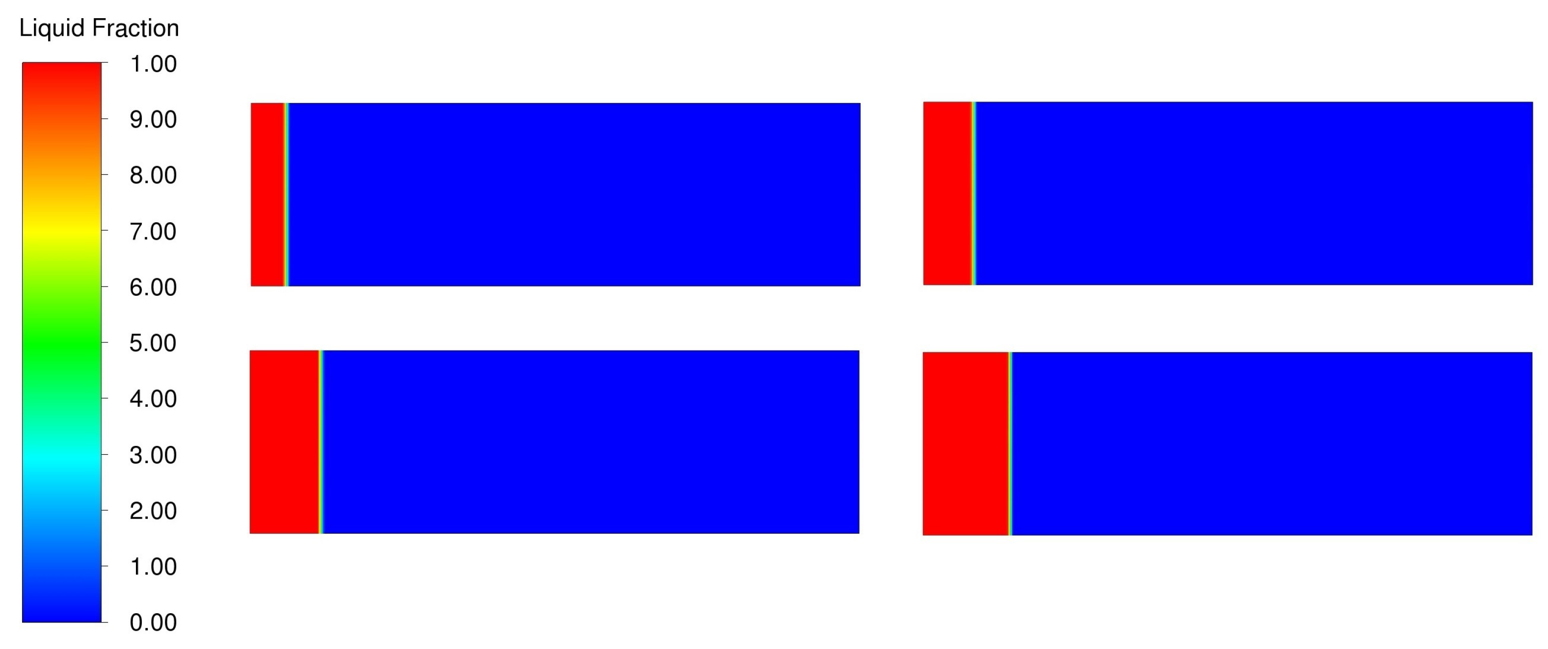
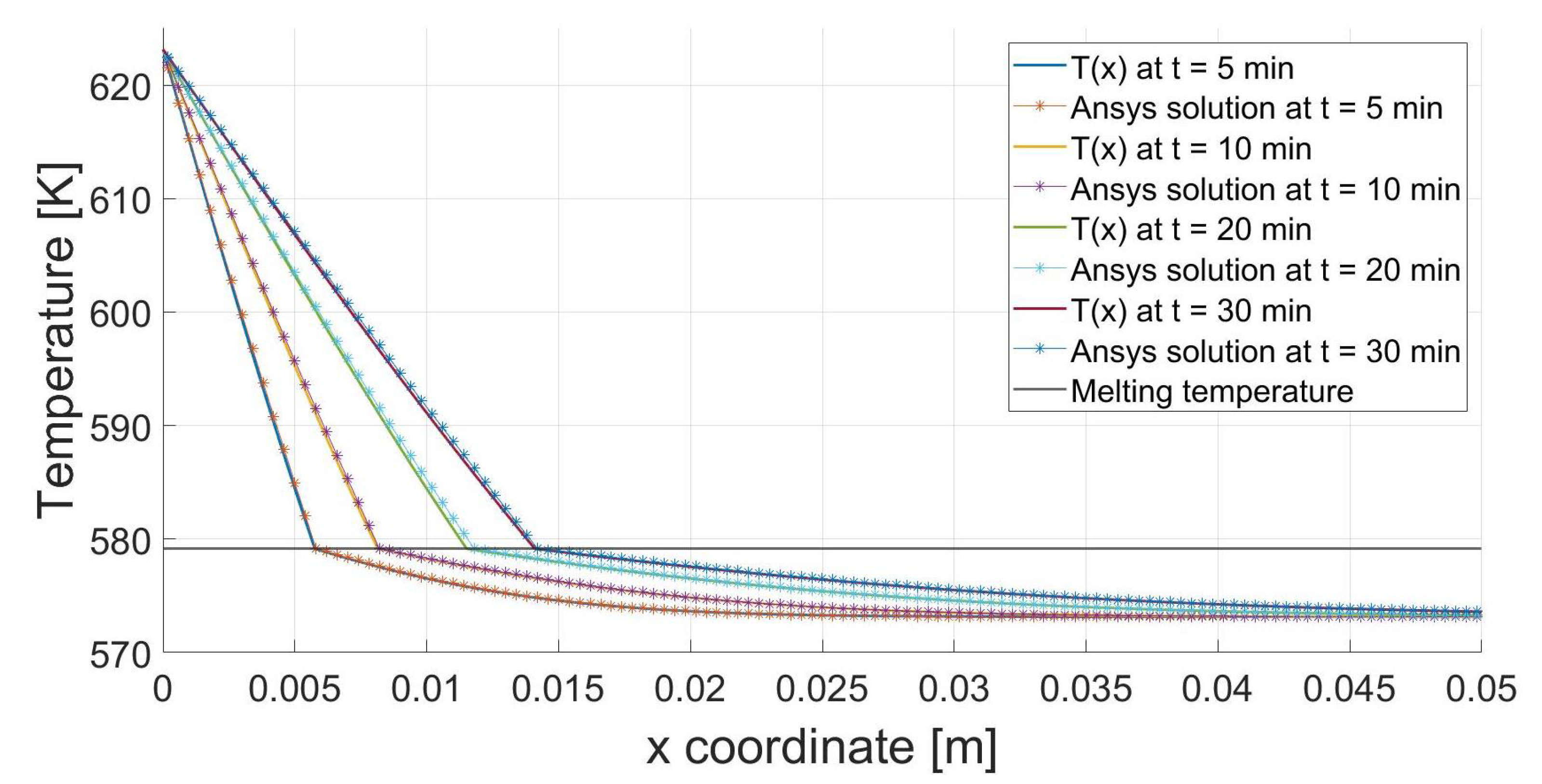
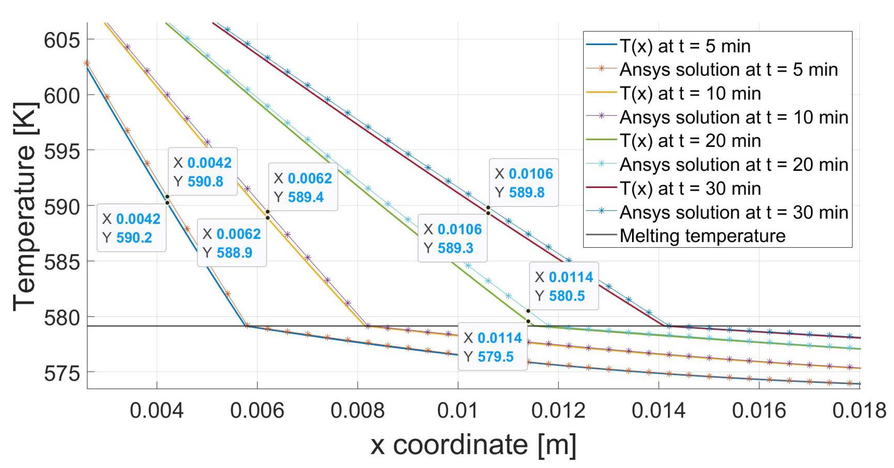
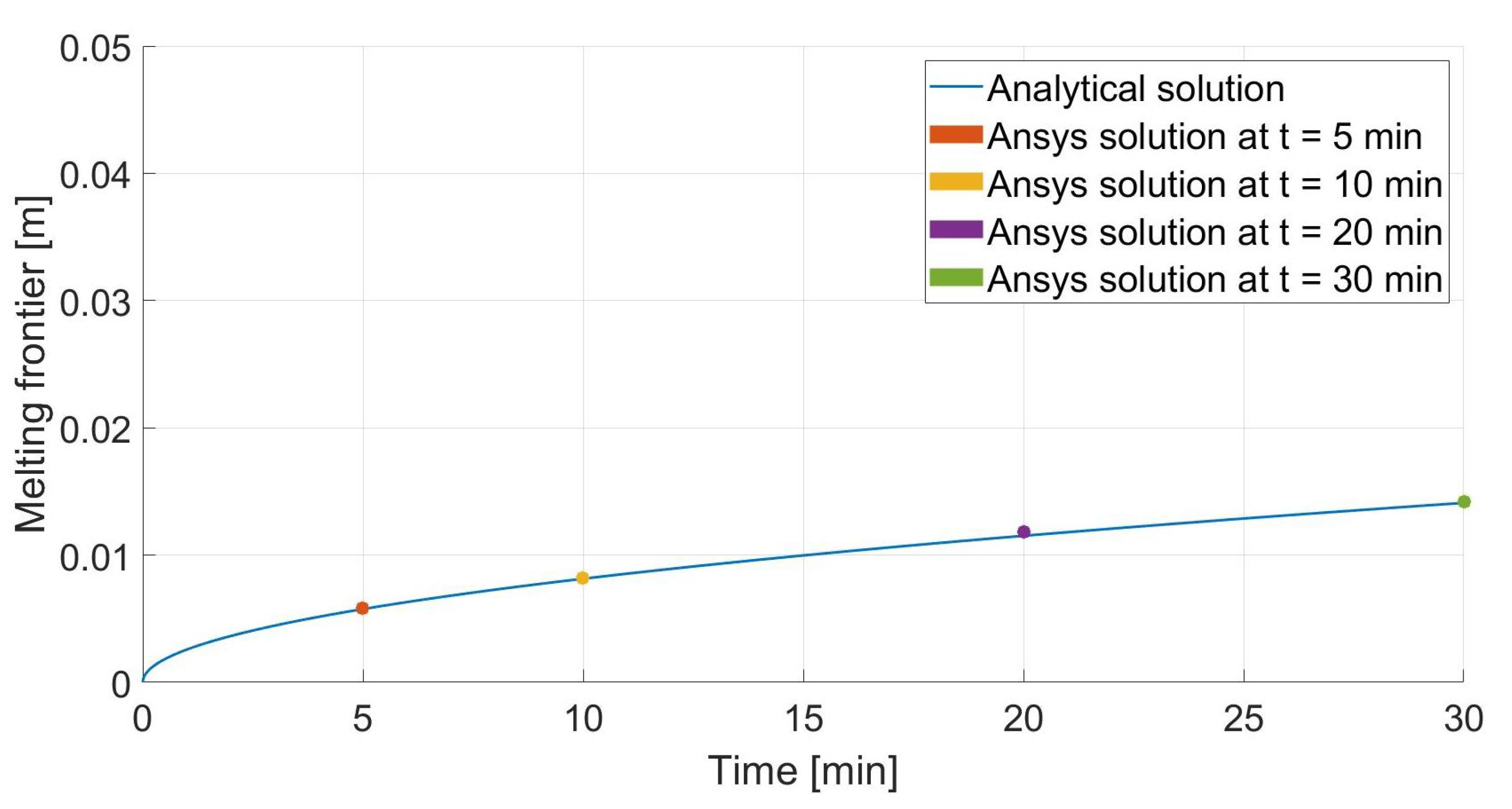
4. Validation of the Numerical Model
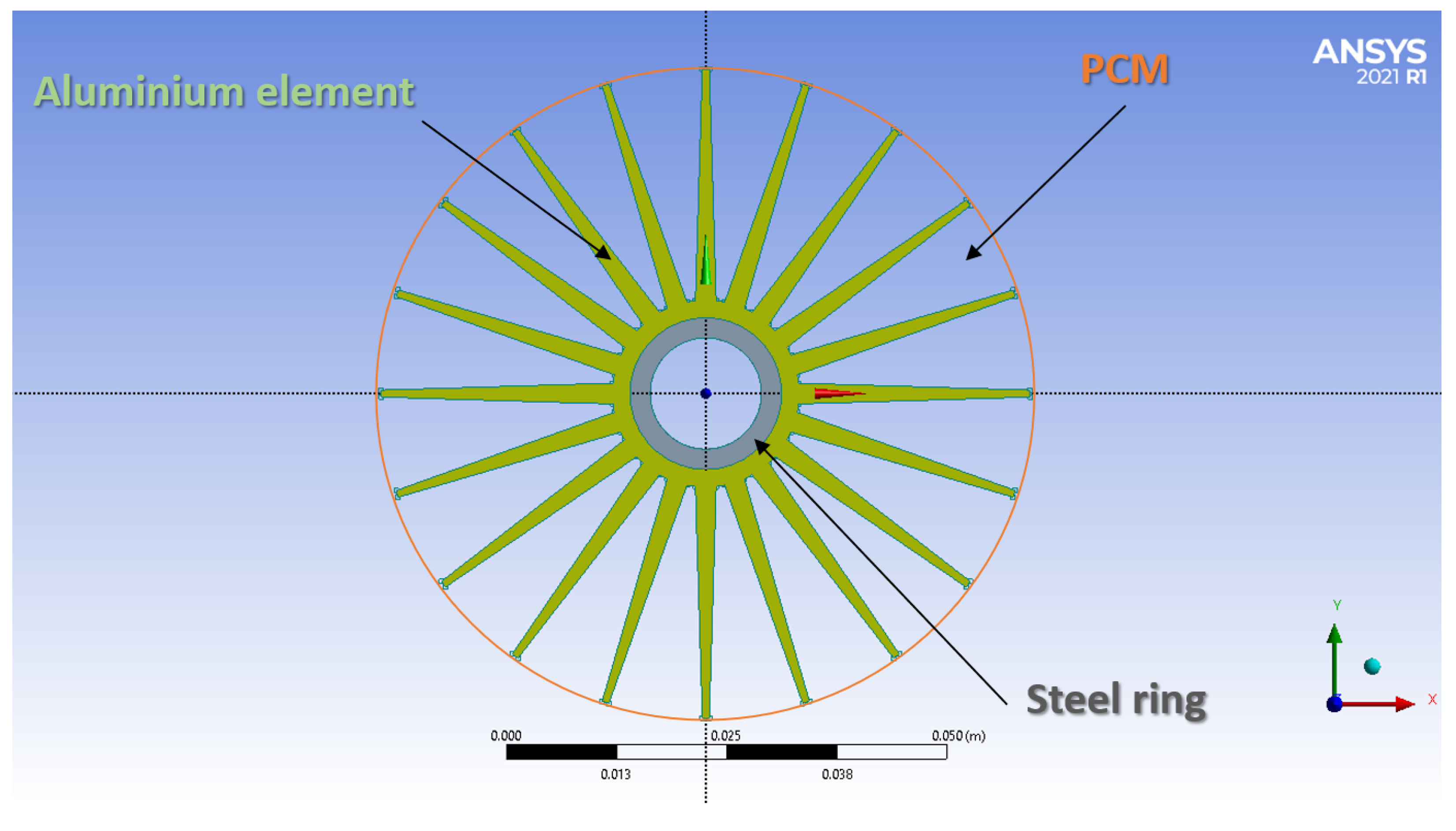
5. Numerical Simulations for the Finned Tube
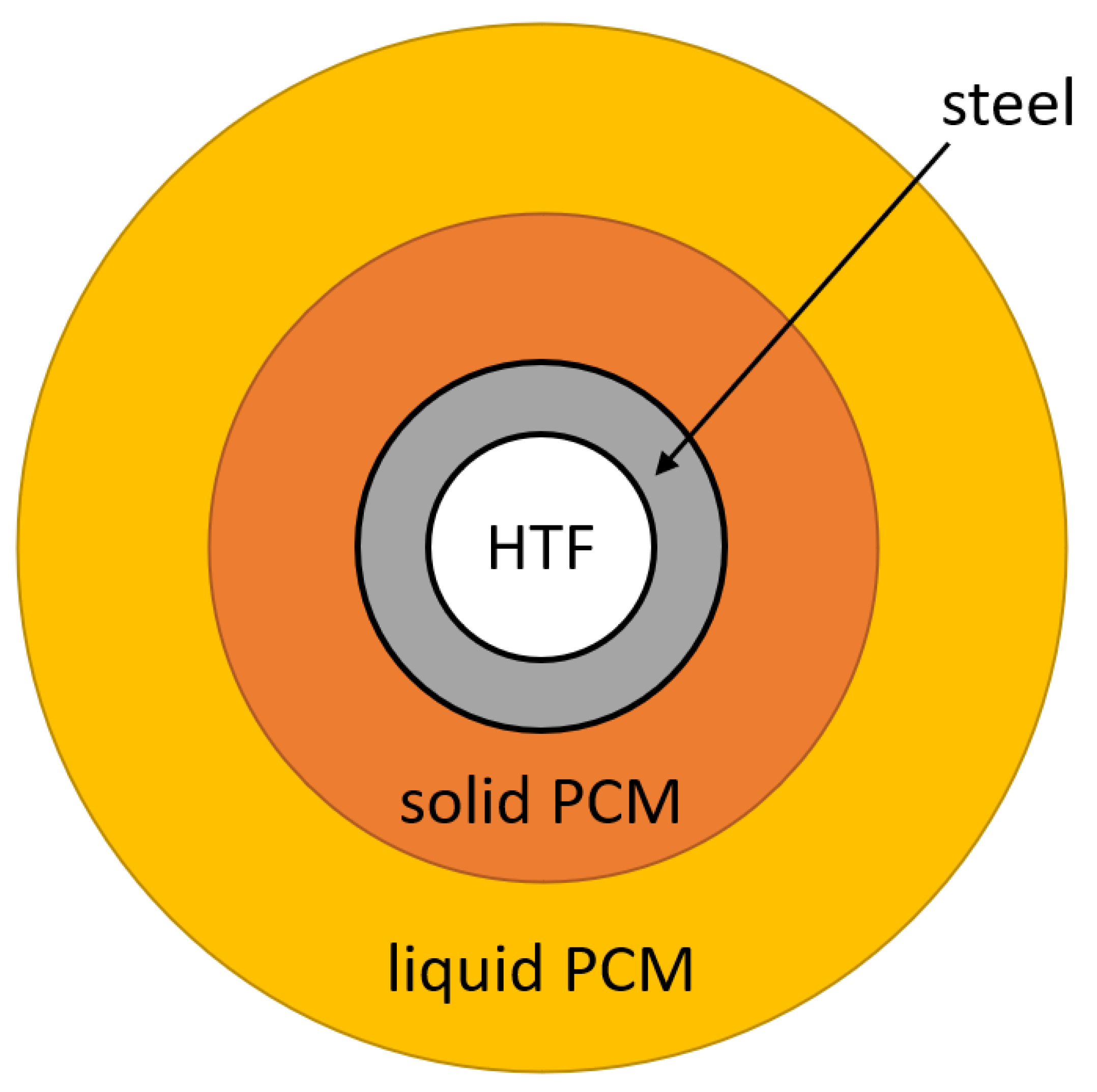
- A steel inner tube in which the heat transfer fluid flows (it does not change in the comparison);
- An aluminium heat conduction structure connected to the heat transfer tube;
- The PCM all around the aluminium structure up to its outer radius.
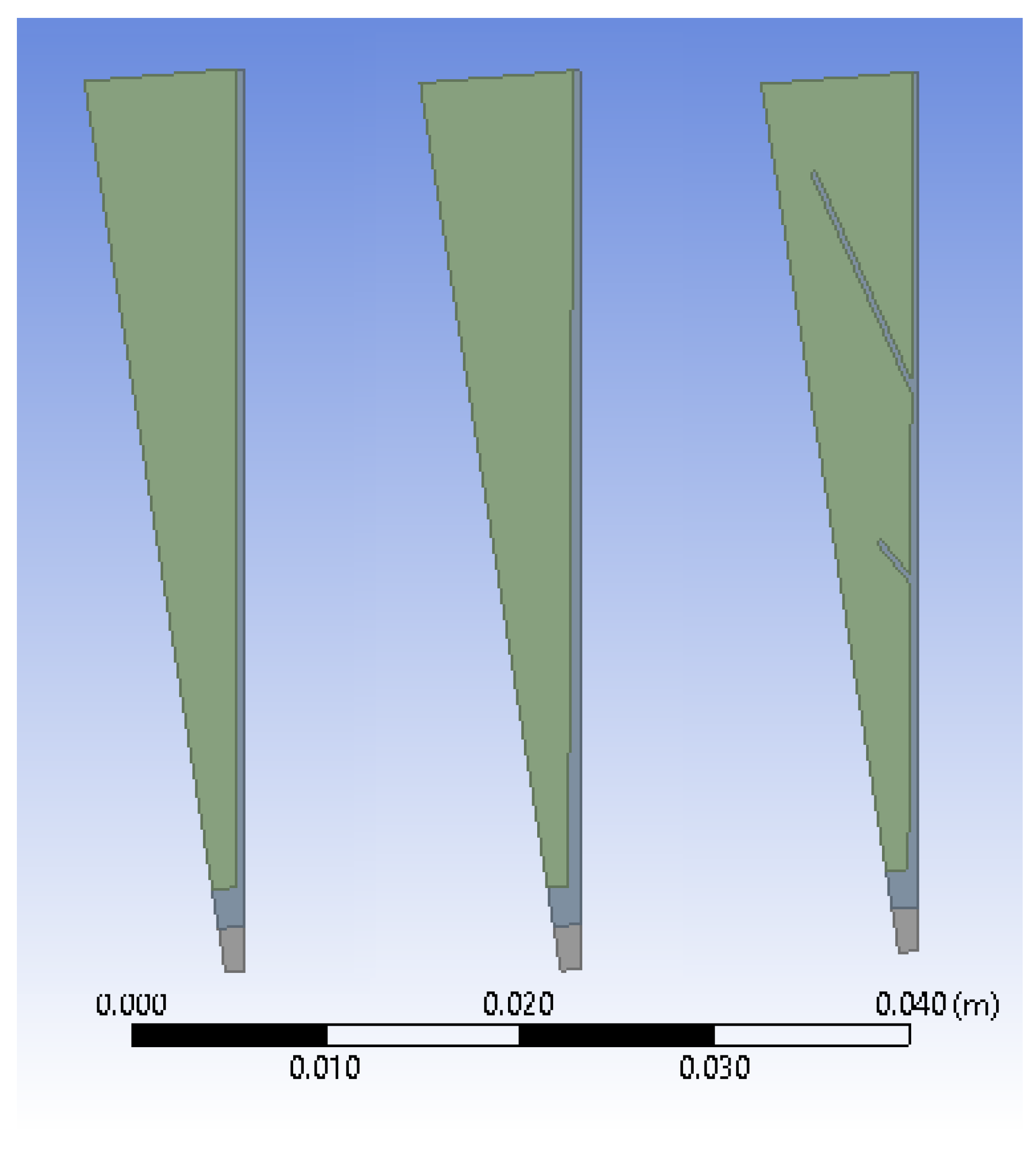
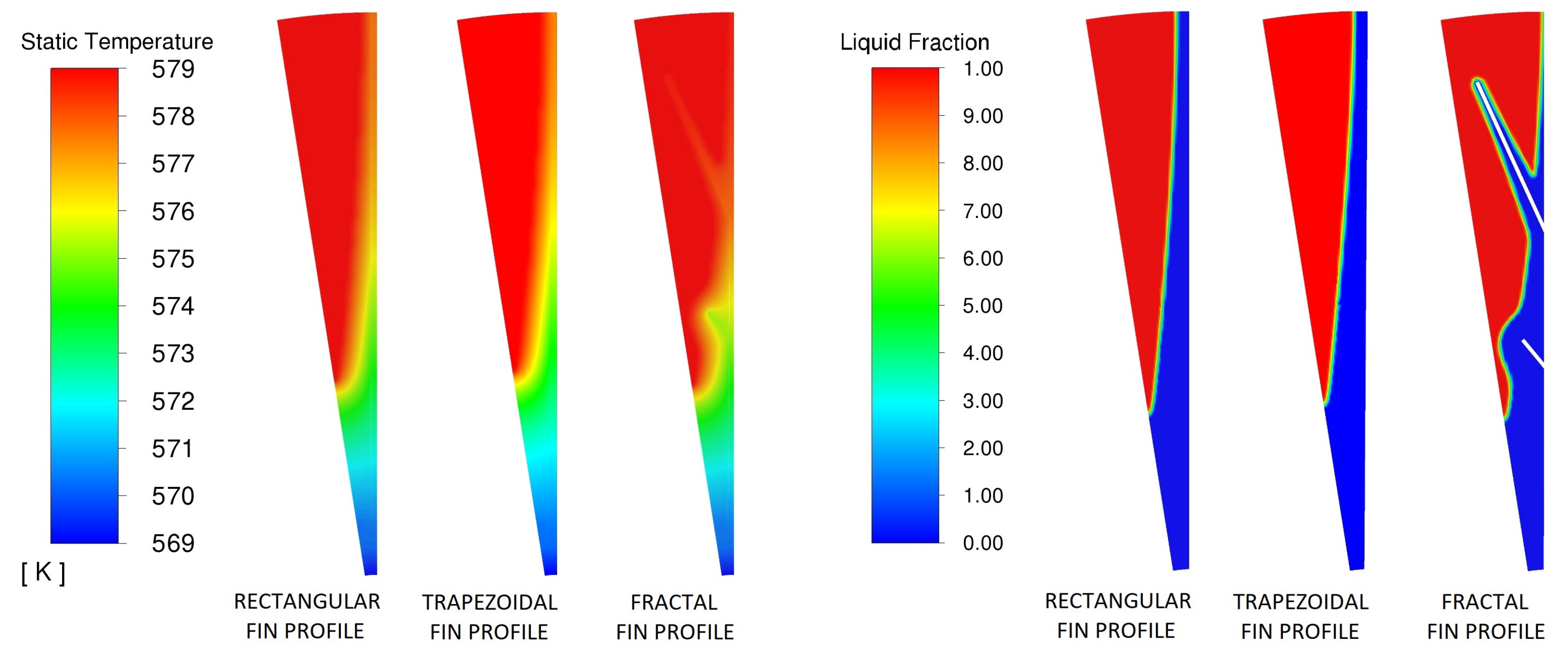
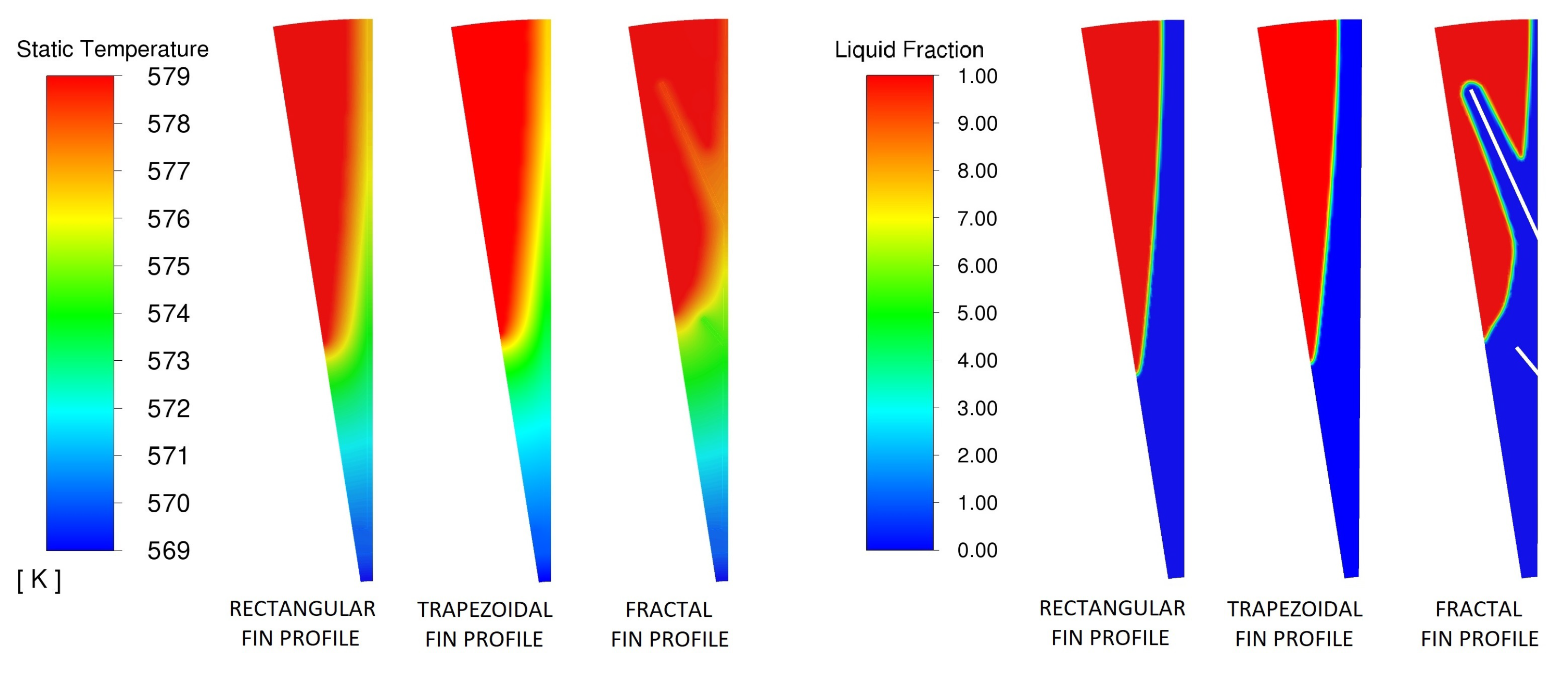
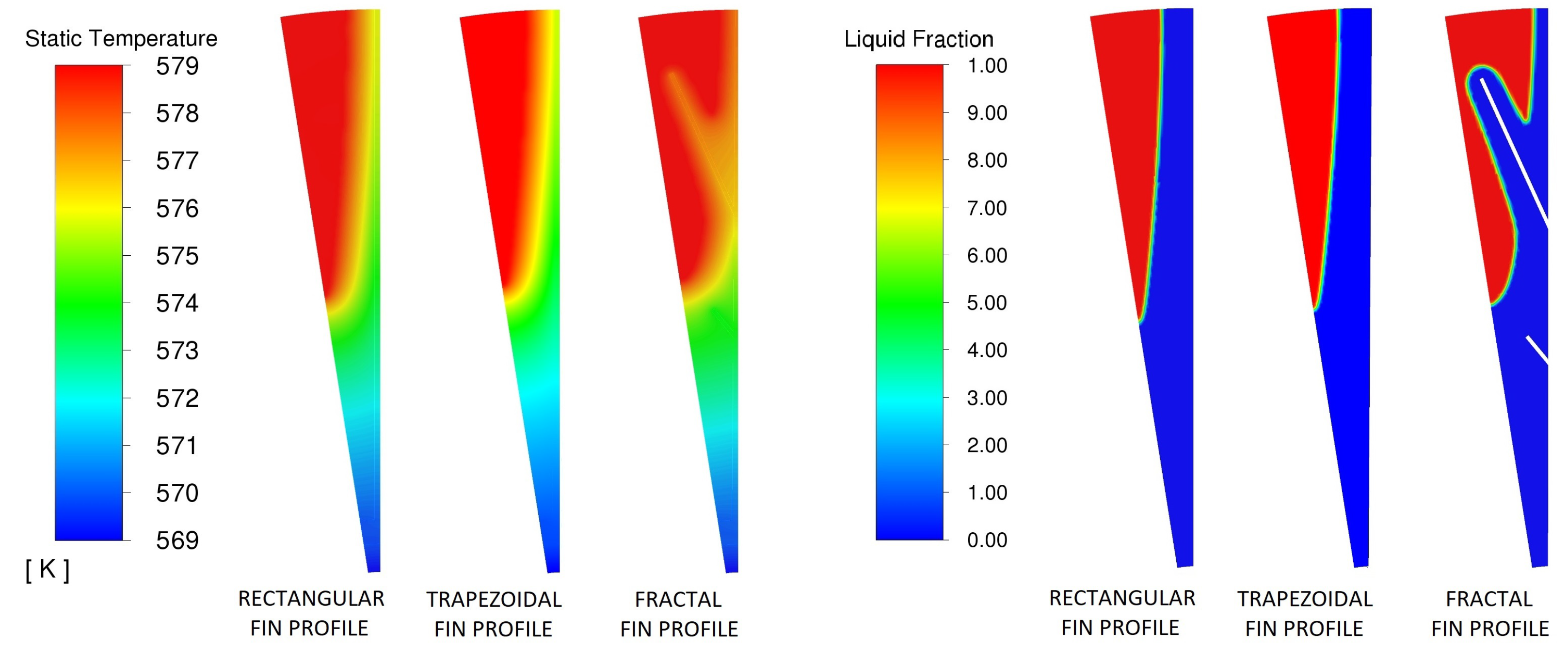
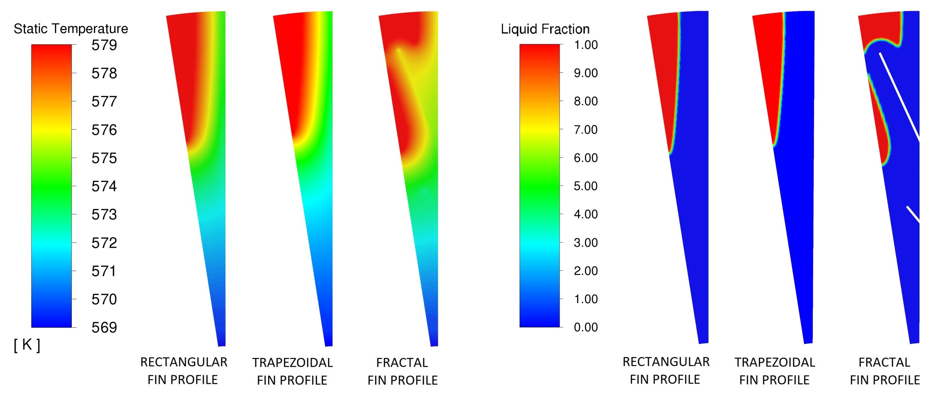
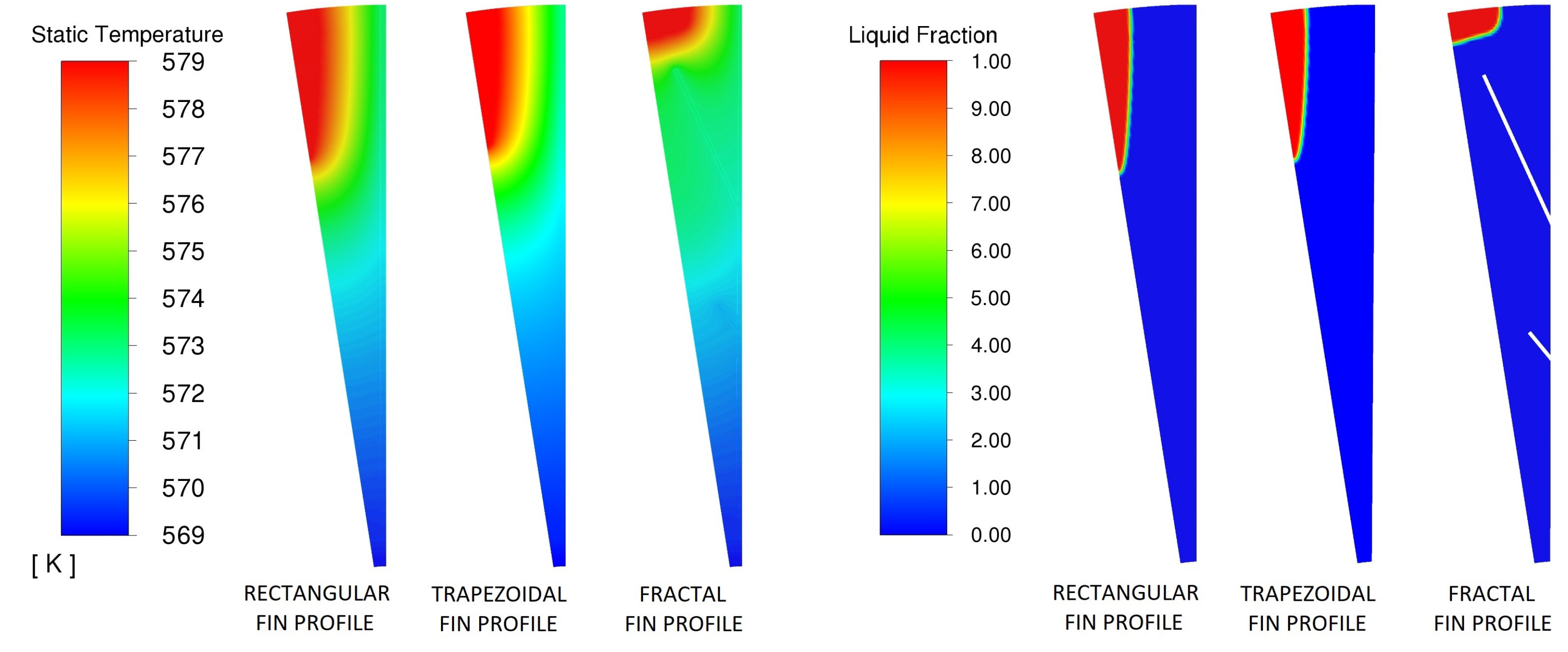
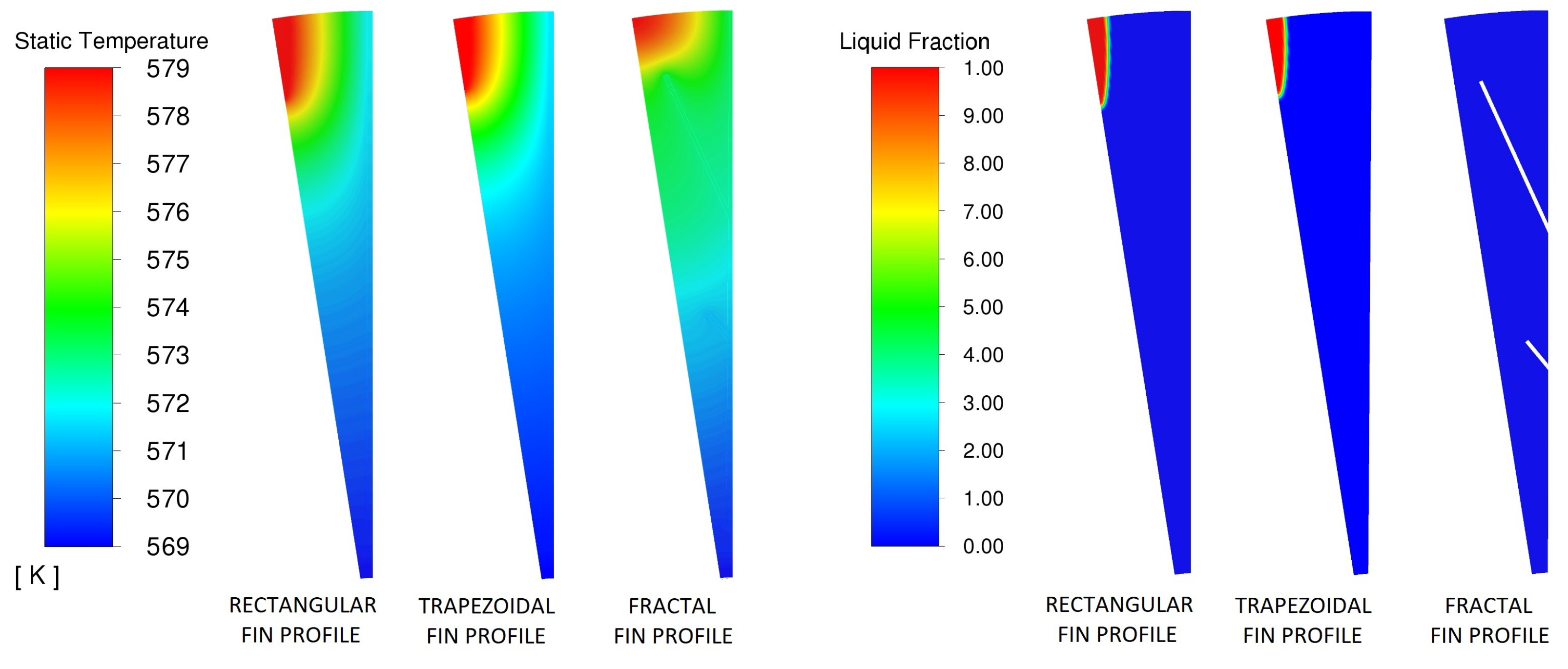
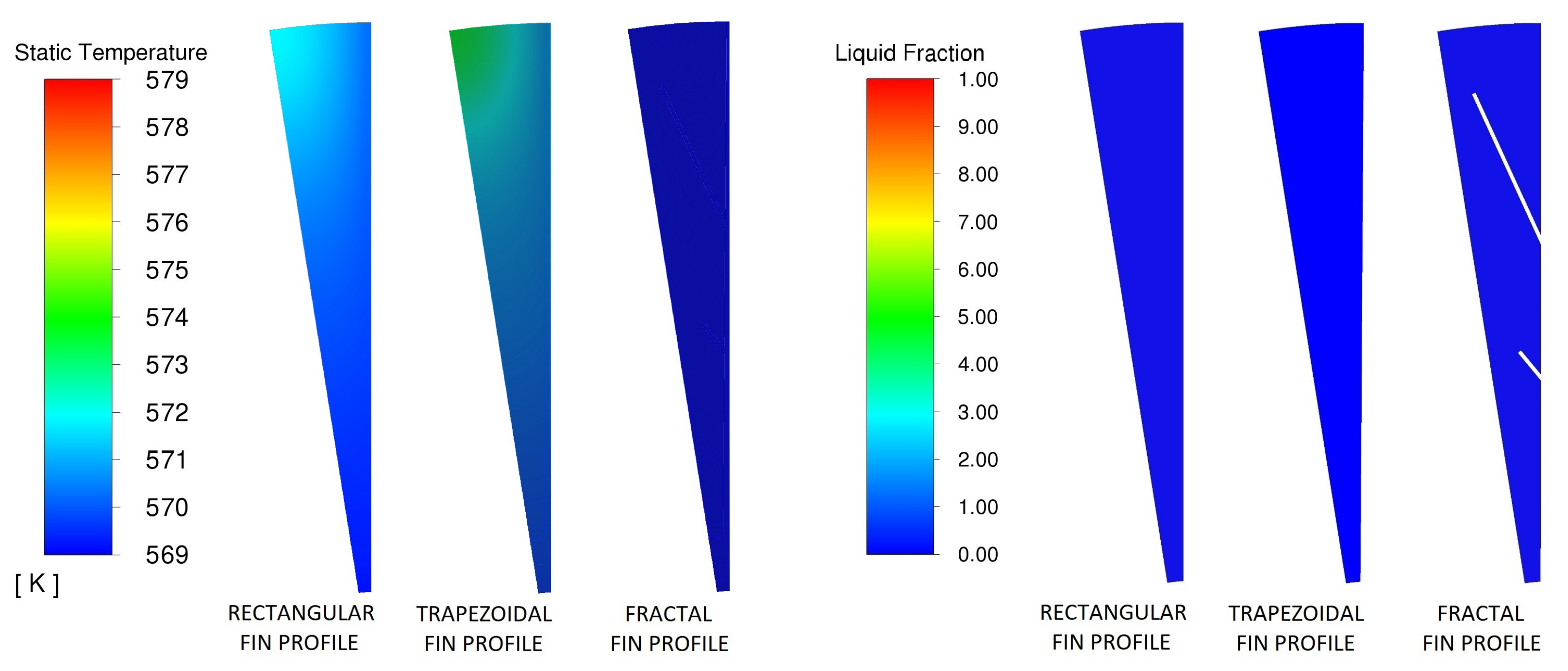
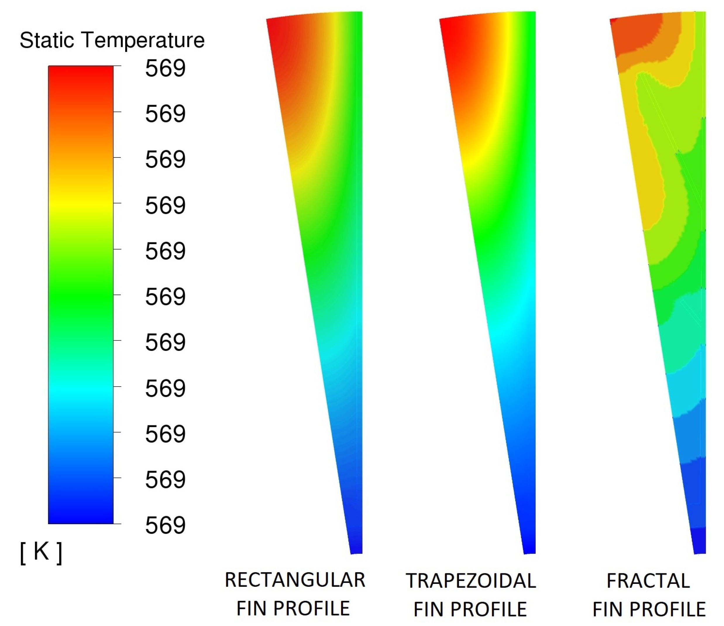
- They change only for the fin shape (rectangular, trapezoidal and fractal fins);
- The three different structures connected to the heat transfer tube have the same volume fraction;
- The PCM mass is constant in all the configurations, which means that the PCM volume fraction is also constant.
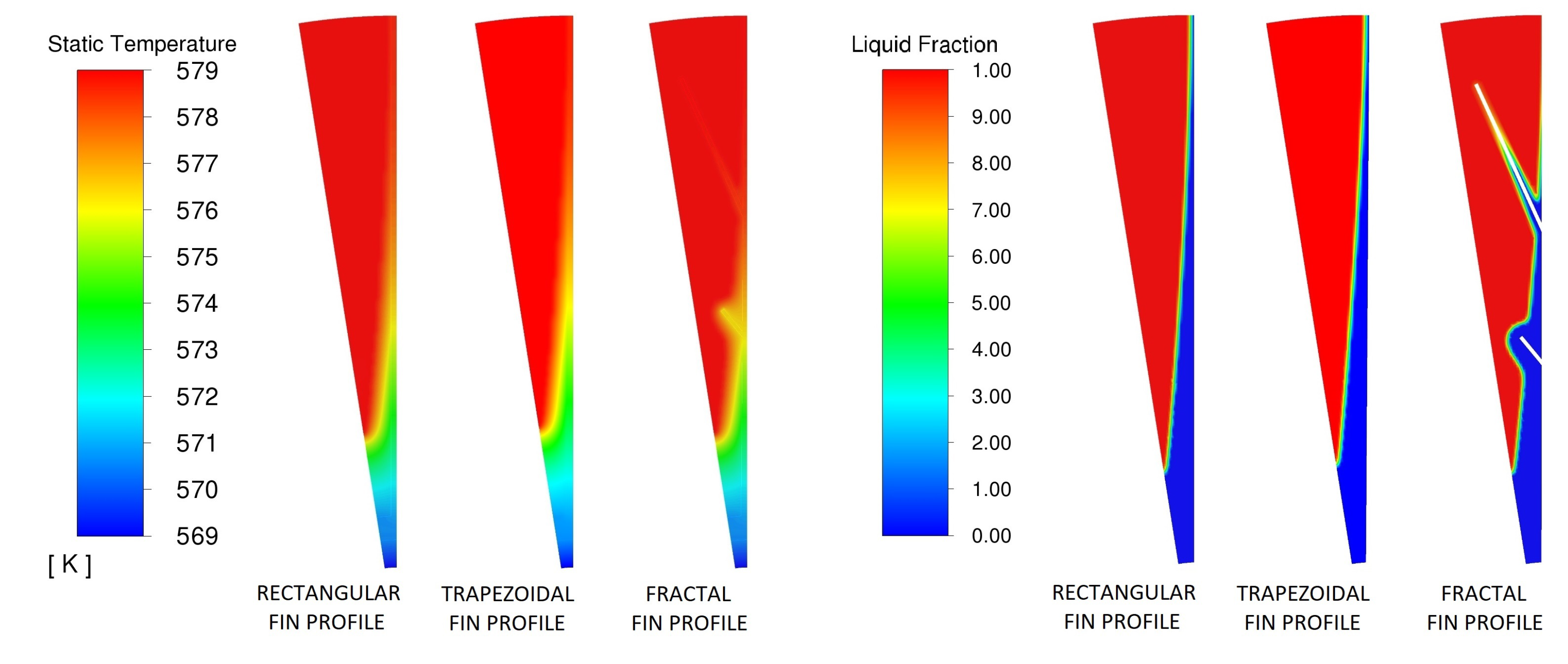
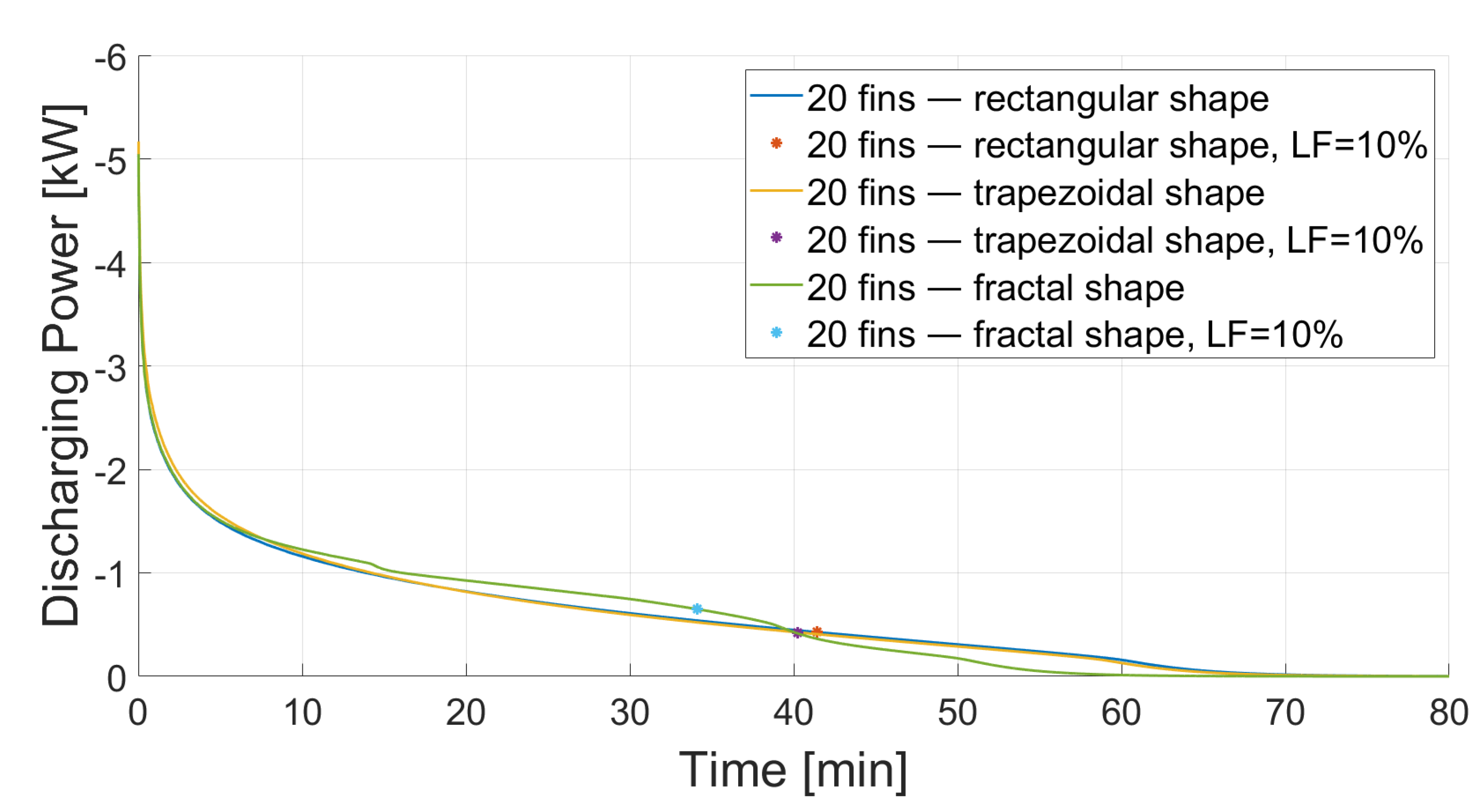
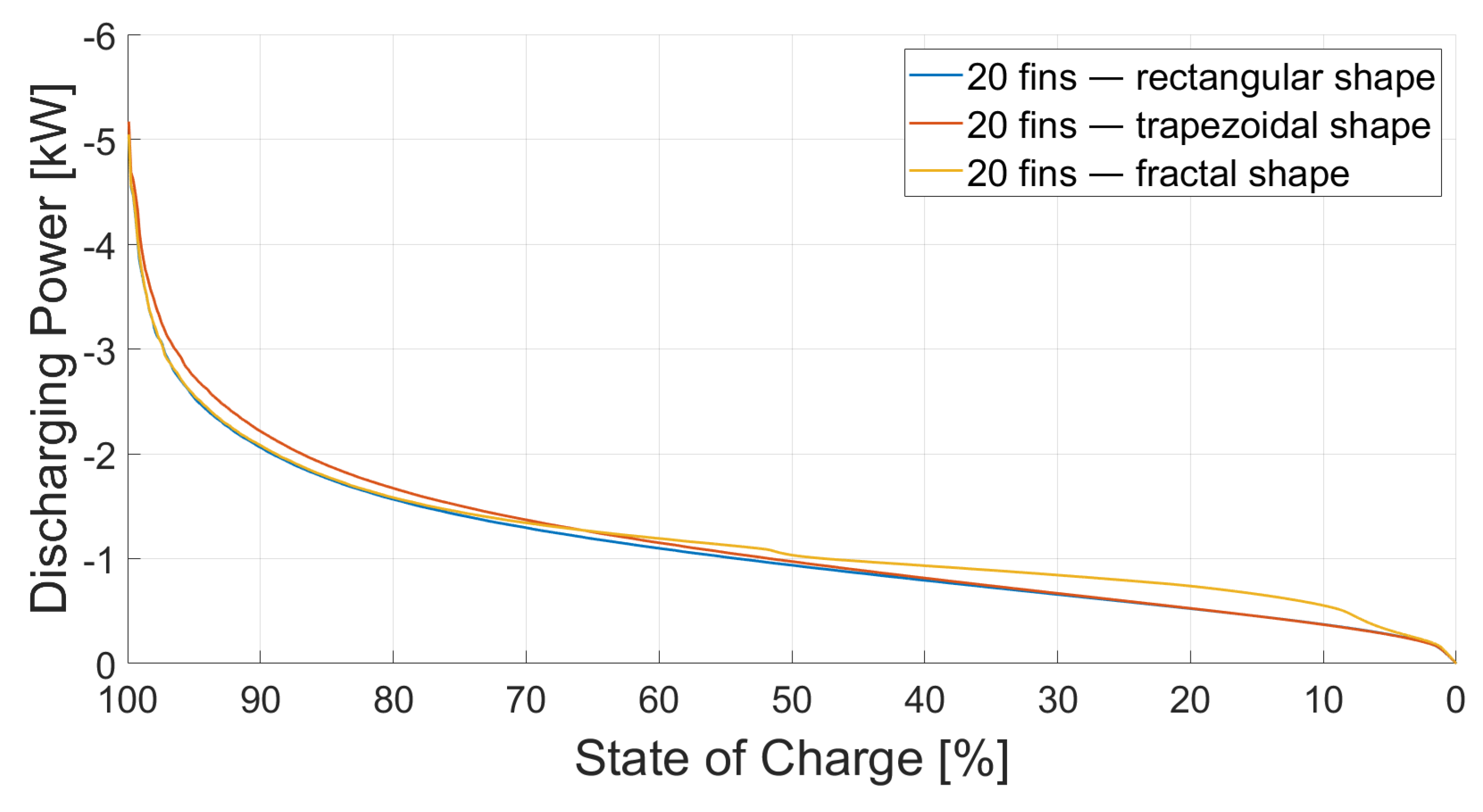
Results and Discussion
- is the time corresponding to LF = 10%;
- is the initial time;
- is the time discretization index;
- is the discharging power corresponding to the i-th time step;
- is the time corresponding to the i-th time step.
- Theoretically aswhere [ ] is the PCM total mass of a 1 length TES system and L ( / ) is the PCM enthalpy of phase change;
- From the discharging power curve (at the inner radius of the steel tube) aswhere is the time corresponding to the end of the simulation, is the time discretization index, is the discharging power corresponding to the i-th time step and is the time corresponding to the time step.
6. Conclusions and Future Developments
Author Contributions
Funding
Data Availability Statement
Acknowledgments
Conflicts of Interest
References
- Gielen, D.; Boshell, F.; Saygin, D.; Bazilian, M.D.; Wagner, N.; Gorini, R. The role of renewable energy in the global energy transformation. Energy Strategy Rev. 2019, 24, 38–50. [Google Scholar] [CrossRef]
- Ley, M.B.; Jepsen, L.H.; Lee, Y.S.; Cho, Y.W.; Bellosta von Colbe, J.M.; Dornheim, M.; Rokni, M.; Jensen, J.O.; Sloth, M.; Filinchuk, Y.; et al. Complex hydrides for hydrogen storage—New perspectives. Mater. Today 2014, 17, 122–128. [Google Scholar] [CrossRef] [Green Version]
- Mackay, D.J. Sustainable Energy—Without the Hot Air; Uit Cambridge Ltd.: Cambridge, UK, 2009. [Google Scholar]
- Trebilcock, F.; Ramirez Stefanou, M.; Pascual, C.; Weller, T.; Lecompte, S.; Hassan, A. Development of a Compressed Heat Energy Storage System Prototype. In Proceedings of the IIR Rankine 2020 Conference—Advances in Cooling, Heating and Power Generation, Virtual, 27–31 July 2020. [Google Scholar] [CrossRef]
- Katsaprakakis, D.A.; Dakanali, I.; Condaxakis, C.; Christakis, D.G. Comparing electricity storage technologies for small insular grids. Appl. Energy 2019, 251, 113332. [Google Scholar] [CrossRef]
- Arnaoutakis, G.E.; Kefala, G.; Dakanali, E.; Katsaprakakis, D.A. Combined Operation of Wind-Pumped Hydro Storage Plant with a Concentrating Solar Power Plant for Insular Systems: A Case Study for the Island of Rhodes. Energies 2022, 15, 6822. [Google Scholar] [CrossRef]
- Elberry, A.; Thakur, J.; Santasalo-Aarnio, A.; Larmi, M. Large-scale compressed hydrogen storage as part of renewable electricity storage systems. Int. J. Hydrogen Energy 2021, 46, 15671–15690. [Google Scholar] [CrossRef]
- Desi-NADINE. 2022. Available online: https://www.igte.uni-stuttgart.de/en/research/research_hrt/completed-projects/desinadine/ (accessed on 10 September 2022).
- Steinmann, W.D.; Jockenhöfer, H.; Bauer, D. Thermodynamic Analysis of High-Temperature Carnot Battery Concepts. Energy Technol. 2020, 8, 1900895. [Google Scholar] [CrossRef] [Green Version]
- Okazaki, T.; Shirai, Y.; Nakamura, T. Concept study of wind power utilizing direct thermal energy conversion and thermal energy storage. Renew. Energy 2015, 83, 332–338. [Google Scholar] [CrossRef] [Green Version]
- Pelay, U.; Luo, L.; Fan, Y.; Stitou, D.; Rood, M. Thermal energy storage systems for concentrated solar power plants. Renew. Sustain. Energy Rev. 2017, 79, 82–100. [Google Scholar] [CrossRef]
- Arnaoutakis, G.E.; Katsaprakakis, D.A.; Christakis, D.G. Dynamic modeling of combined concentrating solar tower and parabolic trough for increased day-to-day performance. Appl. Energy 2022, 323, 119450. [Google Scholar] [CrossRef]
- Innovation Outlook: Thermal Energy Storage. 2022. Available online: https://www.irena.org/publications/2020/Nov/Innovation-outlook-Thermal-energy-storage (accessed on 10 September 2022).
- Brewing Beer with Solar Heat. 2022. Available online: https://www.solarthermalworld.org/sites/default/files/brewing_beer_with_solar_heat.pdf (accessed on 10 September 2022).
- Ortega-Fernández, I.; Rodríguez-Aseguinolaza, J. Thermal energy storage for waste heat recovery in the steelworks: The case study of the REslag project. Appl. Energy 2019, 237, 708–719. [Google Scholar] [CrossRef]
- Turning Waste from Steel Industry into a Valuable Low Cost Feedstock for Energy Intensive Industry. 2022. Available online: https://cordis.europa.eu/project/id/642067 (accessed on 10 September 2022).
- The Parabolic trough Power Plants Andasol 1 to 3. 2022. Available online: http://large.stanford.edu/publications/power/references/docs/Andasol1-3engl.pdf (accessed on 10 September 2022).
- The Project. 2022. Available online: https://www.chester-project.eu/about-chester/the-project/ (accessed on 10 September 2022).
- Laboratory Preparation and Status of the CHEST Technology. 2022. Available online: https://www.chester-project.eu/news/laboratory-preparation-and-status-of-the-chest-technology/ (accessed on 10 September 2022).
- First Thermal Battery Ordered for Commercial Pilot to Decarbonizing Industrial Heating. 2022. Available online: https://www.kyotogroup.no/news/kyoto-group-orders-first-thermal-battery-for-commercial-pilot-decarbonizing-industrial-heat-usage (accessed on 10 September 2022).
- Zalba, B.; Marìn, J.; Cabeza, L.; Mehling, H. Review on thermal energy storage with phase change: Materials, heat transfer analysis and applications. Appl. Therm. Eng. 2003, 23, 251–283. [Google Scholar] [CrossRef]
- Kenisarin, M.M. High-temperature phase change materials for thermal energy storage. Renew. Sustain. Energy Rev. 2010, 14, 955–970. [Google Scholar] [CrossRef]
- Agyenim, F.; Hewitt, N.; Eames, P.; Smyth, M. A review of materials, heat transfer and phase change problem formulation for latent heat thermal energy storage systems (LHTESS). Renew. Sustain. Energy Rev. 2010, 14, 615–628. [Google Scholar] [CrossRef]
- Arnaoutakis, G.E.; Katsaprakakis, D.A. Concentrating Solar Power Advances in Geometric Optics, Materials and System Integration. Energies 2021, 14, 6229. [Google Scholar] [CrossRef]
- Gunasekara, S.; Barreneche, C.; Fernández, A.; Calderon, A.; Ravotti, R.; Ristic, A.; Weinberger, P.; Paksoy, H.; Kocak, B.; Rathgeber, C.; et al. Thermal Energy Storage Materials (TESMs)—What Does It Take to Make Them Fly? Crystals 2021, 11, 1276. [Google Scholar] [CrossRef]
- Jegadheeswaran, S.; Pohekar, S.D. Performance enhancement in latent heat thermal storage system: A review. Renew. Sustain. Energy Rev. 2009, 13, 2225–2244. [Google Scholar] [CrossRef]
- Tamme, R.; Bauer, T.; Buschle, J.; Laing-Nepustil, D.; Müller-Steinhagen, H.; Steinmann, W.D. Latent heat storage above 120 °C for applications in the industral process heat sector and solar power generation. Int. J. Energy Res. 2008, 32, 264–271. [Google Scholar] [CrossRef]
- Al Shannaq, R.; Farid, M. 10—Microencapsulation of phase change materials (PCMs) for thermal energy storage systems. In Advances in Thermal Energy Storage Systems; Woodhead Publishing Series in Energy; Cabeza, L.F., Ed.; Woodhead Publishing: Sawston, UK, 2015; pp. 247–284. [Google Scholar] [CrossRef]
- Dong, K.; Kawaguchi, T.; Shimizu, Y.; Sakai, H.; Nomura, T. Optimized Preparation of a Low-Working-Temperature Gallium Metal-Based Microencapsulated Phase Change Material. ACS Omega 2022, 7, 28313–28323. [Google Scholar] [CrossRef] [PubMed]
- High-Temperature Latent Heat Storage Microcapsules. 2022. Available online: https://seeds.mcip.hokudai.ac.jp/en/view/208/ (accessed on 10 September 2022).
- Ansari, J.A.; Al-Shannaq, R.; Kurdi, J.; Al-Muhtaseb, S.A.; Ikutegbe, C.A.; Farid, M.M. A Rapid Method for Low Temperature Microencapsulation of Phase Change Materials (PCMs) Using a Coiled Tube Ultraviolet Reactor. Energies 2021, 14, 7867. [Google Scholar] [CrossRef]
- Agyenim, F.; Eames, P.; Smyth, M. A comparison of heat transfer enhancement in a medium temperature thermal energy storage heat exchanger using fins. Solar Energy 2009, 83, 1509–1520. [Google Scholar] [CrossRef]
- Stritih, U. An experimental study of enhanced heat transfer in rectangular PCM thermal storage. Int. J. Heat Mass Transfer 2004, 47, 2841–2847. [Google Scholar] [CrossRef]
- Alexiades, V.; Solomon, A. Mathematical Modeling of Melting and Freezing Processes, 1st ed.; Routledge: London, UK, 1993. [Google Scholar]
- 17. Solidification and Melting. 2022. Available online: https://www.afs.enea.it/project/neptunius/docs/fluent/html/th/node349.htm (accessed on 10 September 2022).
- 5.2.1 Heat Transfer Theory. 2022. Available online: https://www.afs.enea.it/project/neptunius/docs/fluent/html/th/node107.htm (accessed on 10 September 2022).
- Cukrov, A.; Sato, Y.; Boras, I.; Ničeno, B. A Solution to Stefan Problem Using Eulerian Two Fluid Vof Model. Brodogr. Teor. Praksa Brodogr. Pomor. Teh. 2021, 72, 141–164. [Google Scholar] [CrossRef]


| NaNO3 | |||
|---|---|---|---|
| Symbol | Property | Solid | Liquid |
| Density | 2010.5 | 2010.5 | |
| c | Specific heat | 1655 | 1655 |
| k | Thermal conductivity | 0.56 | 0.56 |
| L | Enthalpy of phase change | - | 178,000 |
| Melting temperature | 306 | 306 | |
| Error | t = 5 min | t = 10 min | t = 20 min | t = 30 min |
|---|---|---|---|---|
| 1.16% | 1.09% | 1.93% | 1.03% | |
| 0.76% | 0.73% | 2.5% | 0.71% |
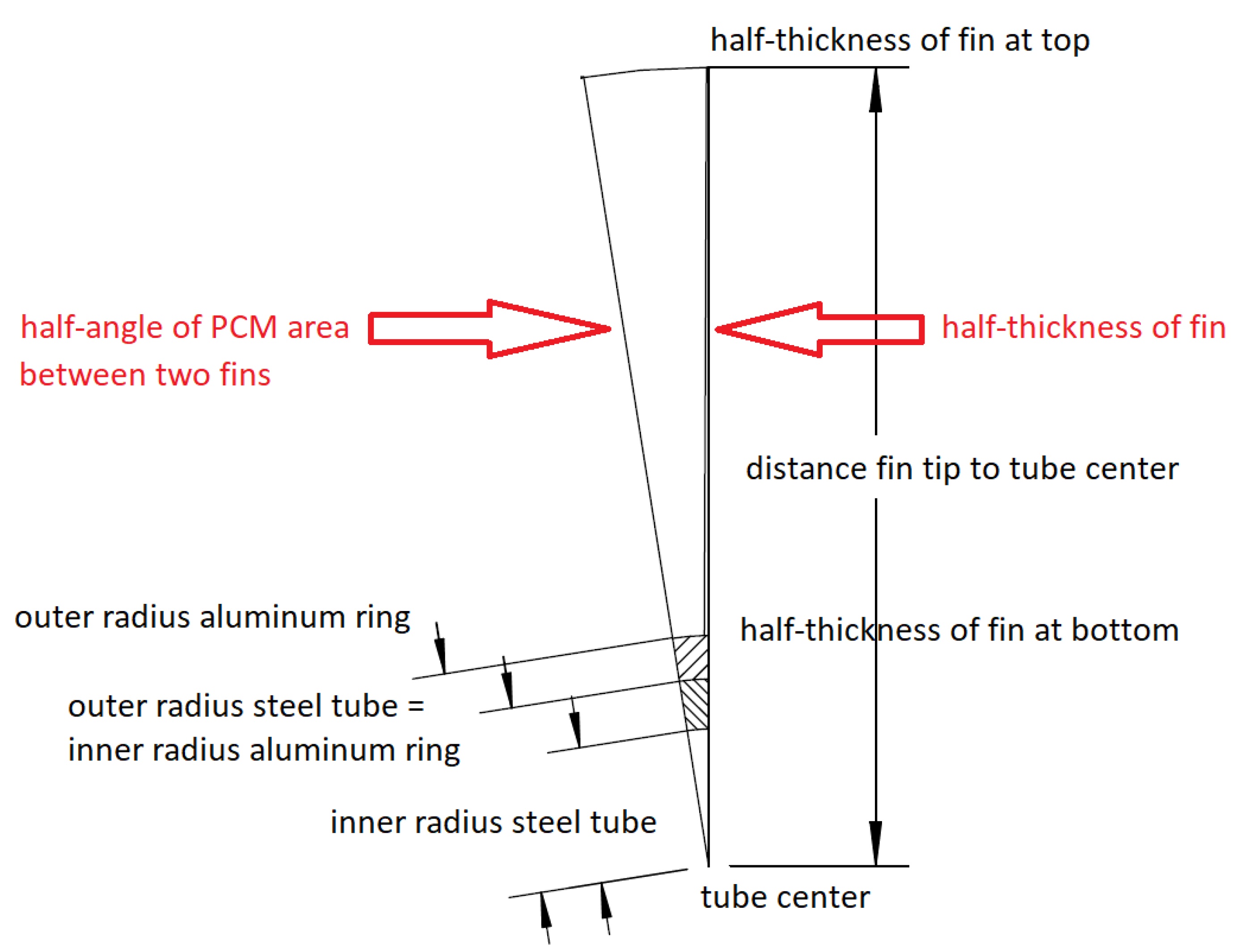
| Material | Characteristic Dimensions | ||
|---|---|---|---|
| Steel ring | 0.0063 | ||
| 0.0086 | |||
| area | 0.0001076616 | m2 | |
| Aluminium ring | 0.0086 | ||
| 0.0106 | |||
| Aluminium fins | number | 20 | |
| 0.0106 | |||
| 0.0525 | m | ||
| Total aluminium structure | area | 0.00091644 | m2 |
| PCM | 0.0106 | ||
| 0.0525 | |||
| area | 0.00751032 | m2 | |
| Rectangular Fins | Trapezoidal Fins | Fractal Fins | |
|---|---|---|---|
| Nodes | 16,409 | 16,622 | 17,096 |
| Elements | 5308 | 5383 | 5543 |
| Rectangular Fins | Trapezoidal Fins | Fractal Fins | |
|---|---|---|---|
| 5 min | 76.16% | 75.00% | 75.94% |
| 10 min | 61.02% | 59.41% | 60.09% |
| 15 min | 48.87% | 47.09% | 46.90% |
| 20 min | 38.71% | 36.94% | 35.51% |
| 30 min | 22.74% | 21.26% | 16.21% |
| 40 min | 11.29% | 10.24% | 4.18% |
| 50 min | 3.62% | 3.01% | 0% |
| 60 min | 0% | 0% | 0% |
| Total Time | Rectangular Fins | Trapezoidal Fins | Fractal Fins | |
|---|---|---|---|---|
| t:LF = 10% | −950.8 W | −979.4 W | −1136.6 W | |
| 80 min | J | J | J | |
| 80 min | J | J | J |
Publisher’s Note: MDPI stays neutral with regard to jurisdictional claims in published maps and institutional affiliations. |
© 2022 by the authors. Licensee MDPI, Basel, Switzerland. This article is an open access article distributed under the terms and conditions of the Creative Commons Attribution (CC BY) license (https://creativecommons.org/licenses/by/4.0/).
Share and Cite
Privitera, E.; Caponetto, R.; Matera, F.; Vasta, S. Impact of Geometry on a Thermal-Energy Storage Finned Tube during the Discharging Process. Energies 2022, 15, 7950. https://doi.org/10.3390/en15217950
Privitera E, Caponetto R, Matera F, Vasta S. Impact of Geometry on a Thermal-Energy Storage Finned Tube during the Discharging Process. Energies. 2022; 15(21):7950. https://doi.org/10.3390/en15217950
Chicago/Turabian StylePrivitera, Emanuela, Riccardo Caponetto, Fabio Matera, and Salvatore Vasta. 2022. "Impact of Geometry on a Thermal-Energy Storage Finned Tube during the Discharging Process" Energies 15, no. 21: 7950. https://doi.org/10.3390/en15217950
APA StylePrivitera, E., Caponetto, R., Matera, F., & Vasta, S. (2022). Impact of Geometry on a Thermal-Energy Storage Finned Tube during the Discharging Process. Energies, 15(21), 7950. https://doi.org/10.3390/en15217950