Abstract
An optimal tilt-angle control based on artificial intelligence (AI control) for tracking bifacial photovoltaic (BPV) systems is developed in this study, and its effectiveness and characteristics are examined by simulating a virtual system over five years. Using deep reinforcement learning (deep RL), the algorithm autonomously learns the control strategy in real time from when the system starts to operate. Even with limited deep RL input variables, such as global horizontal irradiance, time, tilt angle, and power, the proposed AI control successfully learns and achieves a 4.0–9.2% higher electrical-energy yield in high-albedo cases (0.5 and 0.8) as compared to traditional sun-tracking control; however, the energy yield of AI control is slightly lower in low-albedo cases (0.2). AI control also demonstrates a superior performance when there are seasonal changes in albedo. Moreover, AI control is robust against long-term system degradation by manipulating the database used for reward setting.
1. Introduction
Recently, tracking bifacial photovoltaic (BPV) systems have become a mainstream PV technology. In 2021, the market share of BPV cells was 50% and is expected to increase to 85% by 2031 [1]. BPV systems can generate more power per unit module area than monofacial photovoltaic (MPV) systems by generating power from solar radiation that is incident on both the front and rear faces of BPV modules [2,3,4].
The mechanism and control of tracking MPV systems have been studied to generate more power [5,6]. The simplest and most commonly used tracking system is an open-loop system, in which the sun position (solar azimuth and zenith angle) is theoretically calculated and then the system drives the MPV module to directly face the calculated position. Another widely used tracking system is a feedback system, in which photosensors detect the best angle that has the highest solar irradiation. The combination of these two techniques has also been employed. However, few studies for tracking BPV systems have been reported to date.
The modeling and simulation of fixed-installed BPV systems are being studied to improve the energy yield [7,8,9,10,11,12,13,14,15,16,17,18,19,20,21,22]. For instance, Sun et al. investigated the effects of the installation height and ground albedo of BPV modules on the energy yield [15]. Chudinzow et al. estimated the shading effect of adjacent BPV arrays and reported an average annual gain of approximately 17% at a ground albedo of 0.4 [16]. Nussbaumer et al. compared the estimated power by considering the tilt angle of BPV modules and scattered sunlight with the actual measurements and reported that it can be predicted with an error of 2–10% [18]. Rouholamini et al. reported that the power gain of BPV modules compared to MPV modules exceeded 30% in an optimized installation configuration [19].
In addition to the aforementioned fixed-installed systems, BPV systems using single-axis trackers have emerged as a recent development [23,24,25,26,27]. Shoukry et al. reported that a single-axis (one-axis) tracking BPV system yielded approximately 1.4 times the annual energy yield of a fixed MPV system in a region near the equator [23]. A simulation analysis by Rodríguez-Gallegos et al. reported that a one-axis tracking BPV system reduces the levelized cost of electricity (LCOE) by 16% compared to that of a fixed MPV system [25]. Conventional sun-tracking control directs the front surface of the PV module to the sun. However, this may not always be the best control strategy for a tracking BPV system because the output power of the BPV system depends on both the front and rear gains. To the best of our knowledge, there are only a few detailed reports on optimal tilt-angle control for tracking BPV systems [24,27]. Pelaez et al. reported an increase in bifacial gain with an off-sun angle control similar to that used in conventional MPV systems [24]. Moreover, they reported that the optimal tilt angle depends on albedo, latitude, and scattered light. McIntosh et al. reported an optimal tilt-angle determination method using a detailed model-based study [27]. They obtained the irradiance of each solar cell in the modules comprising the array using ray-tracing analysis and estimated the power by considering the current mismatch between the solar cells in the module. Such a model-based approach is useful for BPV systems during the system-design stage. Following the installation of the system, an intelligent tilt-angle controller that autonomously learns the optimal angle may contribute to maximizing power generation because there are many factors affecting the irradiance distribution on the front and rear surfaces of BPV modules. These include the surrounding environment, albedo (e.g., seasonal variations due to snow), angular spectral reflectance of the ground, weather, and partial shadows caused by components and adjacent arrays. Furthermore, there are other uncertain factors. The surrounding environment and system conditions are likely to change during long-term operation. The model-based approach is limited in terms of considering all such possibilities. To address this problem, a data-driven approach is expected to be a solution for optimally controlling the tilt angle under real conditions by self-learning during long-term operations. In this study, a tilt-angle determination algorithm using deep reinforcement learning (deep RL), that is, artificial intelligence (AI) technology, is applied to a one-axis tracking BPV system, and its characteristics and effectiveness were examined during a 5-year simulation of a virtual system. The simulation results show that deep RL autonomously learns the angle-control strategy to achieve a higher power generation than simple sun-tracking. Furthermore, deep RL can respond to seasonal albedo changes and system degradation that conventional tracking methods cannot consider. These results provide a new window of possibilities for AI angle control in BPV systems.
2. Methodology
2.1. Virtual 1-Axis Tracking Bifacial PV Array
A virtual 1-axis tracking BPV array was constructed using PVLib in MATLAB version R2019b [28] to verify the effectiveness of deep RL by simulations. Figure 1 illustrates a model diagram of the virtual system. The installation height (H) from the ground surface to the tracking axis was 5 m, BPV array length (L) was 5 m, and array width was infinitely long and perpendicular to the paper. The tracking axis was along the north–south direction. There were no adjacent BPV arrays.
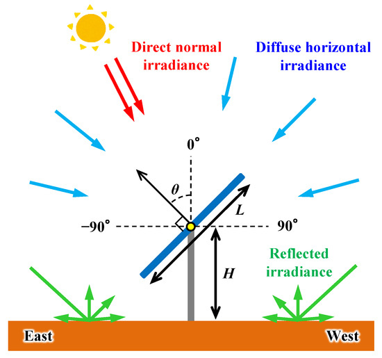
Figure 1.
Diagram of virtual 1-axis tracking bifacial photovoltaic (BPV) array.
Figure 2 displays the calculation flow of the output power of the BPV array. The solar-radiation incident on the front and rear surfaces of the BPV array was calculated using the solar-radiation calculation model, pvl_Purdue_bifacial_irradiance.m [15,29,30], with an array tilt angle (θ), the number of days from 1 January (day of the year: DOY), time (t), albedo (ground surface reflectance against solar radiation), direct normal irradiance (DNI), and diffuse horizontal irradiance (DHI). The code of the model was slightly modified to retain a constant H regardless of θ. The total output power P was the sum of the front and rear powers, which were calculated by multiplying the front and rear irradiance values (IFront, IRear) with the corresponding conversion efficiency (ηFront, ηRear), as shown in Figure 2. The conversion efficiencies of the front and rear surfaces were assumed to be constant values of 19% and 13.3%, respectively, and the bifaciality coefficient = ηRear/ηFront = 0.7, which was based on the specification of the commercial PV modules (Jinko Solar, Tiger Pro 72HC-BDVP). To simplify the computation, temperature changes and other complicated phenomena that could affect the conversion efficiency were ignored. The tilt angle θ was determined at every time step using the deep RL angle controller described in the subsequent section. This virtual array was simple and effective in achieving the objective of the study.
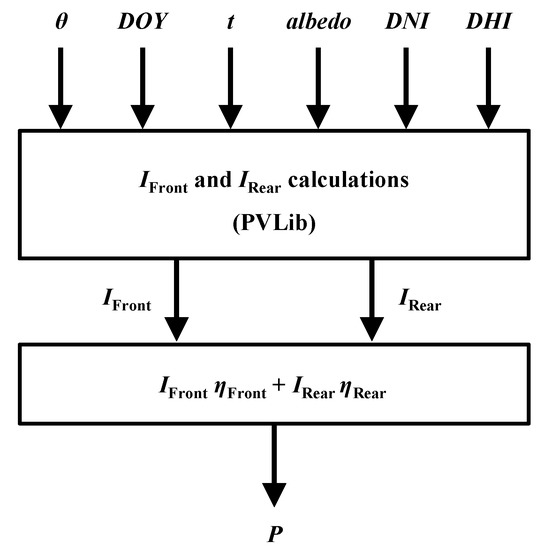
Figure 2.
Schematic of the output-power calculation in virtual 1-axis tracking BPV array.
2.2. Deep RL Angle Controller
Figure 3 illustrates the relationship between the deep RL angle controller and virtual 1-axis tracking BPV array. First, the action selection process described below was performed in the deep RL angle controller based on the output power P at the present time step. Second, the tilt angle θ and output power for the next time step in the virtual array was determined and calculated. To implement this process in a real system, the instantaneous power must be measured by a power conditioner or sensors and transferred to the deep RL controller. Self-learning starts when the virtual array starts the 5-year operation, i.e., deep RL automatically and continuously learns the optimal action that yields more electrical energy based on the experience of controlling the tilt angle and resultant power. The angle controller maximizes the amount of power generation, even in more complicated actual systems, such as those with a temperature change and partial shading modules. In other words, this controller can continue operating regardless of complex factors that influence the amount of power generation.
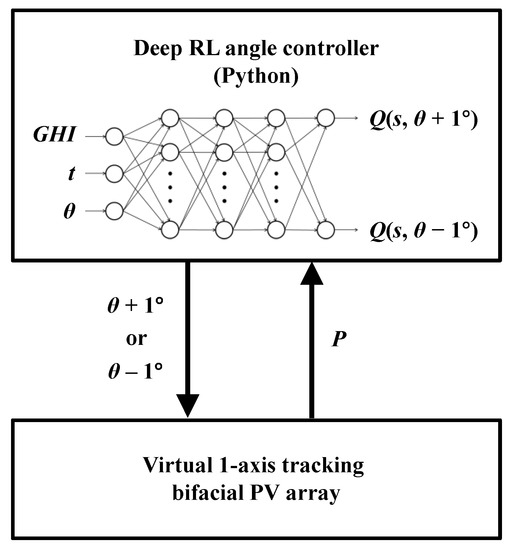
Figure 3.
Data exchange between deep RL angle controller and virtual 1-axis tracking BPV array.
A double deep Q-network (DDQN) [31], a type of deep Q-network [32,33], was employed for the deep RL algorithm. The DDQN solves the overestimation problem of the action-value function when the function approximator of the DQN is utilized. It uses double Q-learning to reduce overestimation by decomposing the target’s maximum action into action selection and action evaluation. In particular, it consists of two Q-networks called main and target. The greedy policy is evaluated according to the main network, whereas the target network is used to estimate its value. The weights of the main network are then replaced by that of the target network for the evaluation of the present greedy policy. Therefore, it exhibits a greater performance than the original DQN and is widely employed [34,35]. It should be noted that a simple feedforward artificial neural network (ANN) based on supervised learning is unsuitable for the present problem because of the difficulty of preparing the training data set. By contrast, RL does not need a training data set and is suitable for the real-time decision of the action.
Table 1 and Figure 4 present the hyperparameters and a diagram of the deep neural network used for the DDQN, respectively. The three input-status variables include global horizontal irradiance (GHI), elapsed time t, and tilt angle θ. In this study, we minimized the number of status variables to reduce the computation time and tuning time of the hyperparameters, and the month and date were not used for the status variable. The set of status variables was defined as s. The DDQN computed the action value Q (s, action) of all possible actions, and the action with the highest Q value was selected. In the present model, there were only two possible actions, θ + 1° or θ − 1°, where θ denotes the tilt angle of a time step. The action value Q was calculated at every time step based on the reward settings in Table 2, while the neural network was simultaneously updated. Here, the values of reward were in the range from 0 to 1 according to the technique called reward clipping, and they were determined by trial and error using the preliminary simulations.

Table 1.
Configuration of deep neural network.
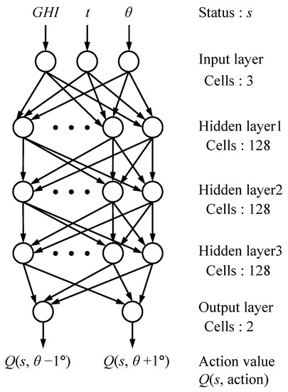
Figure 4.
Schematic of the deep neural network.
Table 2.
Reward settings for deep reinforcement learning.
The power factor (PF) in the table is defined as the ratio of the output power per unit array area to GHI. PFmax indicates the maximum value of PF stored in the database. The database comprises a table with rows and columns for time (2880 bins, in 10-s increments from 8:00 to 16:00) and GHI (1000 bins in total, in 1 W/m2 increments from 0 to 1000 W/m2), respectively, and stores the corresponding PFmax. If the selected action resulted in PF ≥ PFmax, the stored value was updated as PFmax = PF, and the highest reward (1.00) was given for the action, whereas, in the other cases, a negative reward was given.
The deep RL angle controller was programmed using Python. The OpenAI Gym python library was used to implement the DDQN. The simulations were executed using a computer with Intel(R) Core(TM) i7-9700K and 16 GB RAM.
2.3. Simulation Conditions
The simulation conditions are listed in Table 3. Hourly solar-radiation data of GHI, DNI, and DHI for 20 years (1981–2000) in Nagaoka City, Japan (E 138°85′, N 37°45′) from the extended AMeDAS [36] were used for the solar-radiation data. By randomly extracting 5 annual data points from the 20-year dataset and connecting them, 10 consecutive 5-year datasets were created and termed RUN 1–10. The simulation started at 8:00 on 1 January. The simulation time step was set to 10 s. The hourly solar-radiation data were converted into 10-s intervals using linear interpolation. It was assumed that the tracking motor required 10 s to change the tilt angle by 1°. The starting tilt angle in the morning was set to the solar zenith angle at 8:00. For comparison, the output power P with the traditional sun-tracking control was also simulated, where the tilt angle was controlled such that the front surface of the array directly faced the sun. Hereafter, this case is named the “sun-tracking control”, while the angle control using deep RL is named “AI control”. To evaluate the performance of these angle controls, the tilt angle that achieved the highest P at each time step was pre-calculated by simulating P for every tilt angle at 1° intervals and determining the tilt angle with the highest P. This case is named “ideal control”. The ratios of the electrical energy yield (obtained by integrating P over a certain time interval) of AI and sun-tracking controls to that of ideal control are defined as RAI and RSUN, respectively, and collectively termed the energy-yield ratio (R).
Table 3.
Simulation conditions.
3. Simulation Results and Discussion
3.1. 5-Year Simulation
As representative results, Figure 5 illustrates the 5-year variation in daily R for RUNs 1 and 2. The RAI and RSUN are indicated by red and blue dots, respectively. For albedo = 0.2, the AI control showed the same level of performance as the sun-tracking control, whereas for albedo = 0.5, the AI control almost outperformed the sun-tracking control. The efficacy of AI control is even greater for albedo = 0.8, that is, in the high-ground-reflection case. The RSUN fluctuated cyclically and tended to decline during summer. This is because the amount of solar radiation and ground-reflection component increases in summer; however, the RSUN cannot efficiently collect the reflected sunlight at the rear of the array. Comparatively, the RAI exhibited a greater value throughout the year, with some irregular drops. Similar characteristics ere observed in RUNs 3–10, although they are not shown.
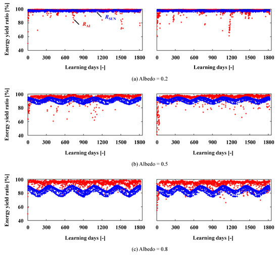
Figure 5.
Variation of daily energy-yield ratio (R) in 5-year simulation (left: RUN 1, right: RUN 2). RAI and RSUN depict the result by AI and sun-tracking controls, respectively.
Figure 6 shows the plots and moving averages of the daily RAIs for RUNs 1–5 in the first 100 days from the start of the operation. Although there are deviations among RUNs, albedo = 0.2 shows the fastest learning progress, exceeding RAI = 0.9 in approximately 20 days. Conversely, albedo = 0.5 and 0.8 tend to take a longer time to learn, that is, 50–60 days to exceed RAI = 0.9. This result indicates that high-ground-reflection cases require a longer learning period in the first year of operation. Interestingly, albedo = 0.5 tends to require the longest period, implying that the difficulty of learning is not simply proportional to the ground-surface reflection’s intensity.
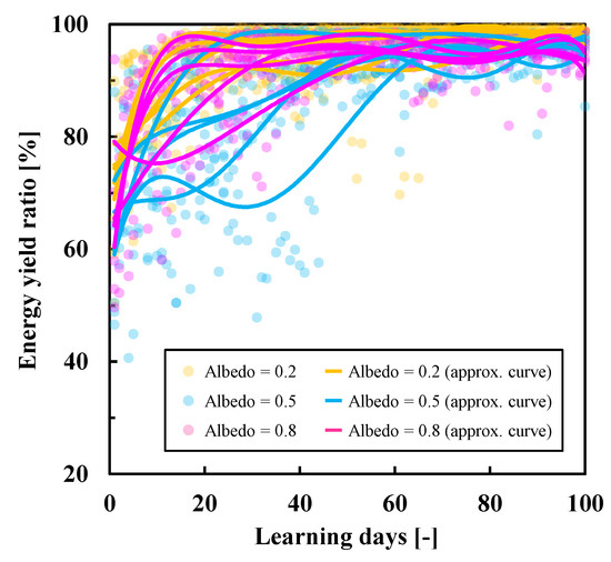
Figure 6.
Variation of daily energy-yield ratio of AI control (RAI) over 100 learning days from the start of the 5-year simulation (RUNs 1–5).
Figure 7 shows a box plot of the daily R for all RUNs. The AI control clearly exhibits a greater energy yield with less diversity than the sun-tracking control, and this trend is more significant for the high-albedo cases, whereas the effectiveness of the AI control is insignificant for the low-albedo case. Even with only three status variables (GHI, t, θ) and output power, AI control shows promising results.
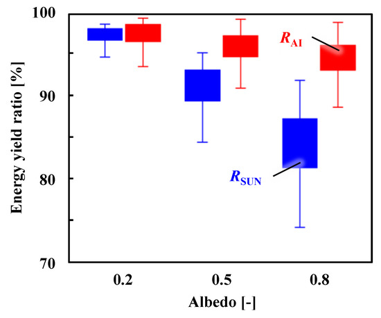
Figure 7.
Box plot of daily energy-yield ratio in 5-year simulation (RUNs 1–10).
Figure 8 shows the 5-year R averaged over all RUNs as a stacked bar graph depicting the breakdown of the front and rear contributions. The AI control shows energy-yield rates of 97.4%, 96.0%, and 94.2% for albedo = 0.2, 0.5, and 0.8, whereas the sun-tracking control shows 98.2%, 92.0%, and 85.0%, respectively. For albedo = 0.2, the AI control is slightly lower than the sun-tracking control; however, for albedo = 0.5 and 0.8, it is 4.0% and 9.2% higher, respectively. The advantage of AI control for high-albedo cases can be attributed to the increase in rear gain. Sun-tracking control cannot effectively utilize the rear gain for high-albedo cases. The decrease in the absolute value of RAI for higher albedo implies that the difficulty of learning increases when the ground-reflection component is high.
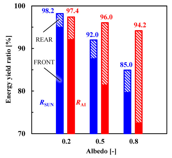
Figure 8.
Stacked bar graph of 5-year energy-yield ratio averaged over RUNs 1–10 with breakdowns of front and rear contributions.
The characteristics of the present AI control can be better understood by observing changes in the tilt angle during the day. Figure 9 illustrates an example of the daily variation in tilt angle and irradiance on a sunny day at the beginning of the operation (day 4) and on a sunny day when learning had sufficiently progressed (day 78). The upper graph in Figure 9 shows a stacking chart of the irradiance on the front (IFRONT) and rear (IREAR) surfaces of the array under AI control and the total irradiance (IIDEAL) on the front and rear surfaces of the array under ideal control. The lower graph in Figure 9 shows the tilt angles under AI (θAI) and ideal (θIDEAL) controls. These graphs present the error of AI control relative to the ideal control. For albedo = 0.2, as shown in Figure 9a, θAI deviates from θIDEAL in the afternoon on day 4, whereas the control nears θIDEAL on day 78; thus, the sum of IFRONT and IREAR approaches IIDEAL. Similar learning progress was observed from days 4 to 78 for high-albedo cases, as shown in Figure 9b,c; however, θAI on day 78 tends to deviate from θIDEAL around noon, and the sum of IFRONT and IREAR becomes lower than IIDEAL. Around noon, a rapid rotation is required to maximize the power because the conversion efficiency of the front is greater than that of the rear (bifaciality coefficient: 0.7); however, AI control does not work well for such a sudden angle change because the tracking motor takes time to rotate the array. If a slower motor is assumed, learning performance and energy yield would be further decreased.
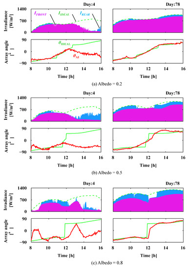
Figure 9.
Comparison of time variation of irradiance and array tilt angle for AI and ideal controls on days 4 and 78. Both days were sunny (RUN 1).
An example of a similar situation, in which AI control is inferior, is depicted in Figure 10. On this day, it was cloudy in the morning and became sunny in the afternoon. Hence, the ideal tilt angle rapidly changed from the negative to positive side close to noon; however, AI control could not follow such a rapid change and maintained the tilt angle on the negative side during the afternoon, resulting in lower irradiance than the ideal control. This was because the present AI control selected the next action to be θ + 1° or θ − 1° and could not jump the tilt angle. Hence, a delay in rotation can result in recovery failure. Overcoming this problem improves the performance of AI control, which may be solved by incorporating solar-radiation forecasting into the AI algorithm.
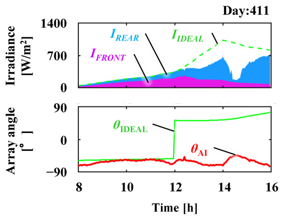
Figure 10.
Time variation on day 411. Cloudy in the morning and sunny in the late afternoon, when AI control works less well (albedo = 0.5, RUN 1).
3.2. Effect of Seasonal Change in Albedo
In the abovementioned simulations, throughout the year, constant values were set for the albedo. However, albedo may vary seasonally, for example, when snow covers the ground or when the ground is covered with artificial high-reflectance sheets for a season when high irradiation is expected. To evaluate the robustness of the AI control against such seasonal changes in albedo, 5-year simulations were performed using the albedo = 0.8 setting between 1 July and 31 August, and albedo = 0.5 for the other periods with three solar radiation datasets RUNs 1–3. The albedo was intentionally set as high during summer when solar radiation is higher to emphasize the effect of albedo change. Figure 11 shows the daily R for RUN 1 as a representative result because the other RUNs exhibit a similar trend. The AI control almost outperforms the sun-tracking control. In particular, during the summer, AI control exhibits a greater energy yield than the sun-tracking control. Figure 12 illustrates the 5-year R averaged over RUNs 1–3. The AI control energy yield is 4.5 percentage points higher than that of the sun-tracking control. This result indicates that AI control is robust to seasonal changes in albedo.
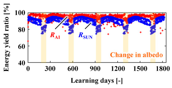
Figure 11.
Variation of daily energy-yield ratio in the case of seasonal albedo changes (albedo = 0.8 from 1 July to 31 August, albedo = 0.5 for the other months, RUN 1).
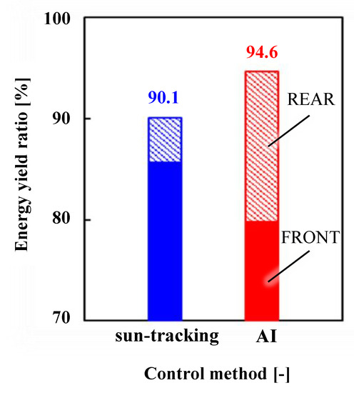
Figure 12.
Five-year energy-yield ratio average over RUNs 1–3 corresponding to Figure 11 (albedo = 0.5).
3.3. Effects of Degradation on Conversion Efficiency
The abovementioned simulations did not consider the degradation of the power-generation performance of the system. However, the conversion efficiency of the actual system deteriorated annually. Considering that it is impossible to stop such deterioration, it would be interesting to determine whether AI control is robust against such long-term-performance degradation. Figure 13 presents the simulation results of daily R when applying a degradation rate of −10%/year for RUN 1 at every time step. The extreme degradation rate was intentionally set, as this was a sensitivity analysis. The actual degradation rate of real PV systems is generally much lower than this value. The graph clearly shows that degradation negatively affects the learning performance of AI control. This problem was primarily caused by the database used in the reward setting. As explained in Section 3, the rewards for the selected action were determined based on whether the PFmax recorded in the database was exceeded by the PF contributed by the selected action. Indeed, this procedure does not work correctly when the PF gradually declines owing to degradation because PFmax is never exceeded by the new actions’ PF and is never updated. A solution to this problem is to manipulate PFmax in the database to decrease the value by a similar degradation rate.
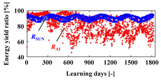
Figure 13.
Variation of daily energy-yield ratio when applying a conversion efficiency degradation rate of −10%/year (albedo = 0.5, RUN 1).
Figure 14 presents the simulation results when database manipulations are applied to the simulation described in Figure 13. In this simulation, the degradation rate (−10%/year) was applied to the conversion efficiency, and as a countermeasure for this degradation, all PFmax values recorded in the database were manipulated to decrease by ratios of (a) −5%/year and (b) −15%/year at every time step. The results reveal that the database manipulation of −15%/year successfully solved the problem, i.e., the 5-year RAI recovered to 94.3% from 78.9% (Figure 13); however, manipulating the database by −5%/year was insufficient. These results indicate that an effective solution is to apply a greater decrease rate for the PFmax value in the database than the actual degradation rate of the system’s power-generation performance.
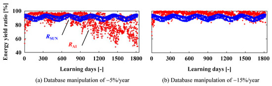
Figure 14.
Effect of PFmax value manipulation in the database for the same simulation as in Figure 13.
4. Conclusions
In this study, the effectiveness of deep RL for optimally controlling the tilt angle of a one-axis tracking bifacial PV array was verified through a 5-year simulation of a virtual system. Even with a minimal number of the status variable inputs to the deep neural network, AI control with deep RL resulted in greater power and electrical energy yields for high-albedo cases (albedo = 0.5 and 0.8) compared to a simple sun-tracking control. AI control was also robust to seasonal albedo changes and the long-term degradation of the system. It is expected that the effectiveness of deep RL will be more promising in complex real-world systems (e.g., systems with multiple arrays) than existing simple virtual system because deep RL automatically learns the optimal angle regardless of the complex factors influencing power generation in real time. Conversely, the deep RL challenges yet to be tackled are to accelerate learning from when the system starts operating, to respond better to the demands of rapid rotation, and to suppress the chattering behavior of the motor operating the array angle. Modifying the deep neural network with more status variables and incorporating solar-radiation forecasting may provide solutions. Explorations of the best algorithms are also necessary through comparative studies to clarify the superiority of AI control. In addition to the simulations, experimental studies are essential to develop a better algorithm and verify its practical performance.
Author Contributions
Conceptualization, N.Y.; methodology, H.N. and N.Y.; software, S.T.; validation, H.N. and S.T.; formal analysis, S.T.; data curation, S.T.; writing—original draft preparation, S.T. and N.Y.; writing—review and editing, H.N.; visualization, H.N.; supervision, N.Y.; project administration, N.Y. All authors have read and agreed to the published version of the manuscript.
Funding
This research received no external funding.
Institutional Review Board Statement
Not applicable.
Informed Consent Statement
Not applicable.
Data Availability Statement
All data and material are available upon reasonable request.
Acknowledgments
We thank Takushi Uchida and Yuki Yamagata, who are graduates from the Energy Engineering Laboratory at Nagaoka University of Technology, for their efforts in the development of the programming code in the early stages of this research.
Conflicts of Interest
The authors declare no conflict of interest.
References
- VDMA. International Technology Roadmap for Photovoltaic (ITPRV). Available online: https://www.vdma.org/international-technology-roadmap-photovoltaic (accessed on 22 October 2022).
- Deline, C.; Macalpine, S.; Marion, B.; Toor, F.; Asgharzadeh, A.; Stein, J.S. Assessment of bifacial photovoltaic module power rating methodologies—Inside and out. IEEE J. Photovolt. 2017, 7, 575–580. [Google Scholar] [CrossRef]
- Zhang, Y.; Yu, Y.; Meng, F.; Liu, Z. Experimental investigation of the shading and mismatch effects on the performance of bifacial photovoltaic modules. IEEE J. Photovolt. 2020, 10, 296–305. [Google Scholar] [CrossRef]
- Raina, G.; Vijay, R.; Sinha, S. Study on the optimum orientation of bifacial photovoltaic module. Int. J. Energy Res. 2022, 46, 4247–4266. [Google Scholar] [CrossRef]
- AL-Rousan, N.; Isa, N.A.M.; Desa, M.K.M. Advances in solar photovoltaic tracking systems: A review. Renew. Sust. Energ. Rev. 2018, 82, 2548–2569. [Google Scholar] [CrossRef]
- Hafez, A.Z.; Yousef, A.M.; Harag, N.M. Solar tracking systems: Technologies and trackers drive types—A review. Renew. Sust. Energ. Rev. 2018, 91, 754–782. [Google Scholar] [CrossRef]
- Guo, S.; Walsh, T.M.; Peters, M. Vertically mounted bifacial photovoltaic modules: A global analysis. Energy 2013, 61, 447–454. [Google Scholar] [CrossRef]
- Yusufoglu, U.A.; Lee, T.H.; Pletzer, T.M.; Halm, A.; Koduvelikulathu, L.J.; Comparotto, C.; Kopecek, R.; Kurz, H. Simulation of energy production by bifacial modules with revision of ground reflection. Energy Procedia 2014, 55, 389–395. [Google Scholar] [CrossRef]
- Yusufoglu, U.A.; Pletzer, T.M.; Koduvelikulathu, L.J.; Comparotto, C.; Kopecek, R.; Kurz, H. Analysis of the annual performance of bifacial modules and optimization methods. IEEE J. Photovolt. 2015, 5, 320–328. [Google Scholar] [CrossRef]
- Lindsay, A.; Chiodetti, M.; Binesti, D.; Mousel, S.; Lutun, E.; Radouane, K.; Christopherson, J. Modelling of single-axis tracking gain for bifacial PV systems. In Proceedings of the 32nd EU PVSEC, European Photovoltaic Solar Energy Conference and Exhibition, Munich, Germany, 20–24 June 2016; pp. 1610–1617. [Google Scholar]
- Di Stefano, A.; Leotta, G.; Bizzarri, F. LA Silla PV plant as a utility-scale side-by-side test for innovative modules technologies. In Proceedings of the 33rd European Photovoltaic Solar Energy Conference and Exhibition, Amsterdam, The Netherlands, 25–29 September 2017; pp. 1978–1982. [Google Scholar]
- Marion, B.; MacAlpine, S.; Deline, C.; Asgharzadeh, A.; Toor, F.; Riley, D.; Stein, J.; Hansen, C. A practical irradiance model for bifacial PV modules. In Proceedings of the 2017 IEEE 44th Photovoltaic Specialist Conference (PVSC), Washington, DC, USA, 25–30 June 2018; pp. 1537–1542. [Google Scholar] [CrossRef]
- Khan, M.R.; Hanna, A.; Sun, X.; Alam, M.A. Vertical bifacial solar farms: Physics, design, and global optimization. Appl. Energy 2017, 206, 240–248. [Google Scholar] [CrossRef]
- Stein, J.S.; Riley, D.; Lave, M.; Hansen, C.; Deline, C.; Toor, F. Outdoor field performance from bifacial photovoltaic modules and systems. In Proceedings of the 2017 IEEE 44th Photovoltaic Specialist Conference (PVSC), Washington, DC, USA, 25–30 June 2017; pp. 3184–3189. [Google Scholar] [CrossRef]
- Sun, X.; Khan, M.R.; Deline, C.; Alam, M.A. Optimization and performance of bifacial solar modules: A global perspective. Appl. Energy. 2018, 212, 1601–1610. [Google Scholar] [CrossRef]
- Chudinzow, D.; Haas, J.; Díaz-Ferrán, G.; Moreno-Leiva, S.; Eltrop, L. Simulating the energy yield of a bifacial photovoltaic power plant. Sol. Energy. 2019, 183, 812–822. [Google Scholar] [CrossRef]
- Patel, M.T.; Khan, M.R.; Sun, X.; Alam, M.A. A worldwide cost-based design and optimization of tilted bifacial solar farms. Appl. Energy 2019, 247, 467–479. [Google Scholar] [CrossRef]
- Nussbaumer, H.; Janssen, G.; Berrian, D.; Wittmer, B.; Klenk, M.; Baumann, T.; Baumgartner, F.; Morf, M.; Burgers, A.; Libal, J.; et al. Accuracy of simulated data for bifacial systems with varying tilt angles and share of diffuse radiation. Sol. Energy 2020, 197, 6–21. [Google Scholar] [CrossRef]
- Rouholamini, M.; Chen, L.; Wang, C. Modeling, configuration, and grid integration analysis of bifacial PV arrays. IEEE Trans. Sustain. Energy 2021, 12, 1242–1255. [Google Scholar] [CrossRef]
- Robledo, J.; Robledo, J.; Leloux, J.; Sarr, B.; Gueymard, C.A.; Driesse, A.; Drouin, P.-F.; Ortega, S.; André, D. Lessons Learned from Simulating the Energy Yield of an Agrivoltaic Project with Vertical Bifacial Photovoltaic Modules in France Quantification and Forecasting of PV Power Fluctuations View Project PV System Simulation Software Validation View Project Les. 2021. Available online: https://www.researchgate.net/publication/354630592 (accessed on 24 October 2022).
- Riaz, M.H.; Imran, H.; Younas, R.; Butt, N.Z. The optimization of vertical bifacial photovoltaic farms for efficient agrivoltaic systems. Sol. Energy 2021, 230, 1004–1012. [Google Scholar] [CrossRef]
- Barbosa, J.D.; Ansari, A.S.; Manandhar, P.; Qureshi, O.A.; Rodriguez Ubinas, E.I.; Alberts, V.; Sgouridis, S. Tilt correction to maximize energy yield from bifacial PV modules. In Proceedings of the IOP Conference Series: Earth and Environmental Science, 6th International Conference on Energy and Environmental Science, Kuala Lumpur, Malaysia, 6–8 January 2022; Volume 1008, p. 012008. [Google Scholar] [CrossRef]
- Shoukry, I.; Libal, J.; Kopecek, R.; Wefringhaus, E.; Werner, J. Modelling of Bifacial Gain for Stand-alone and in-field Installed Bifacial PV Modules. Energy Procedia 2016, 92, 600–608. [Google Scholar] [CrossRef]
- Pelaez, S.A.; Deline, C.; Greenberg, P.; Stein, J.S.; Kostuk, R.K. Model and validation of single-axis tracking with bifacial PV. IEEE J. Photovolt. 2019, 9, 715–721. [Google Scholar] [CrossRef]
- Rodríguez-Gallegos, C.D.; Liu, H.; Gandhi, O.; Singh, J.P.; Krishnamurthy, V.; Kumar, A.; Stein, J.S.; Wang, S.; Li, L.; Reindl, T.; et al. Global techno-economic performance of bifacial and tracking photovoltaic systems. Joule 2020, 4, 1514–1541. [Google Scholar] [CrossRef]
- Rodriguez-Gallegos, C.D.; Gandhi, O.; Panda, S.K.; Reindl, T. On the PV tracker performance: Tracking the sun versus tracking the best orientation. IEEE J. Photovolt. 2020, 10, 1474–1480. [Google Scholar] [CrossRef]
- McIntosh, K.R.; Abbott, M.D.; Sudbury, B.A. The optimal tilt angle of monofacial and bifacial modules on single-axis trackers. IEEE J. Photovolt. 2022, 12, 397–405. [Google Scholar] [CrossRef]
- Stein, J.S.; Holmgren, W.F.; Forbess, J.; Hansen, C.W. PVLIB: Open source photovoltaic performance modeling functions for MATLAB and Python. In Proceedings of the 2016 IEEE 43th Photovoltaic Specialists Conference (PVSC), Portland, OR, USA, 5–10 June 2016; pp. 3425–3430. [Google Scholar]
- Martín, N.; Ruiz, J.M. Annual angular reflection losses in PV modules. Prog. Photovolt. Res. Appl. 2005, 13, 75–84. [Google Scholar] [CrossRef]
- Sandia National Laboratories. pvl_Purdue_bifacial_irradiance.m. Available online: https://github.com/sandialabs/MATLAB_PV_LIB/ (accessed on 22 October 2022).
- Van Hasselt, H.; Guez, A.; Silver, D. Deep reinforcement learning with double Q-learning. In Proceedings of the AAAI Conference on Artificial Intelligence, Phoenix, AZ, USA, 12–17 February 2016. [Google Scholar] [CrossRef]
- Mnih, V.; Kavukcuoglu, K.; Silver, D.; Graves, A.; Antonoglou, I.; Wierstra, D.; Riedmiller, M. Playing Atari with Deep Reinforcement Learning. arXiv 2013, arXiv:1312.5602. Available online: http://arxiv.org/abs/1312.5602 (accessed on 24 October 2022).
- Mnih, V.; Kavukcuoglu, K.; Silver, D.; Rusu, A.A.; Veness, J.; Bellemare, M.G.; Graves, A.; Riedmiller, M.; Fidjeland, A.K.; Ostrovski, G.; et al. Human-level control through deep reinforcement learning. Nature 2015, 518, 529–533. [Google Scholar] [CrossRef] [PubMed]
- Lei, X.; Zhang, Z.; Dong, P. Dynamic path planning of unknown environment based on deep reinforcement learning. J. Robot. 2018, 2018, 5781591. [Google Scholar] [CrossRef]
- Ning, B.; Lin, F.H.T.; Jaimungal, S. Double Deep Q-Learning for Optimal Execution. arXiv 2018, arXiv:1812.06600. Available online: http://arxiv.org/abs/1812.06600 (accessed on 24 October 2022). [CrossRef]
- Meteorological Data System Co., Ltd. Extended AMeDAS Meteorological Data. Available online: https://www.metds.co.jp/business_list/ (accessed on 24 October 2022).


Publisher’s Note: MDPI stays neutral with regard to jurisdictional claims in published maps and institutional affiliations. |
© 2022 by the authors. Licensee MDPI, Basel, Switzerland. This article is an open access article distributed under the terms and conditions of the Creative Commons Attribution (CC BY) license (https://creativecommons.org/licenses/by/4.0/).