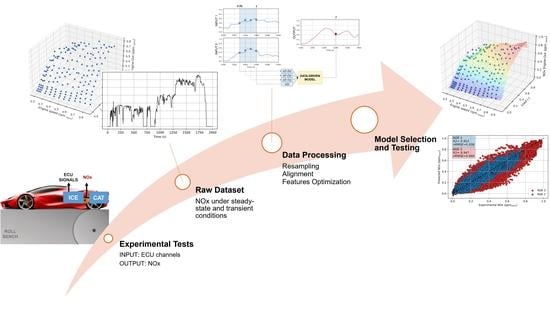
1. Introduction
These days, due to the increasing number of sensors installed on the engine and the high number of experimental tests, the amount of data available for the car manufacturers is always wider. This, along with the enhancement of computational power of common devices, is affecting the way with which data are managed, processed and analyzed [
1].
To extract insights from such a high amount of data, Artificial Intelligence (AI) techniques are also spreading in the automotive fields, especially for applications related to autonomous driving, vehicle control, smart connections, virtual sensing and fault diagnosis [
2].
The AI models are computationally cheap and capable of learning the main characteristics of systems based only on experimental measurements, without requiring explicit programming, thus reducing the effort required to model complex physical and chemical phenomena [
3,
4]. Moreover, the ability to process large amounts of information in a short time and to learn system behavior from experimental data makes AI models interesting for many applications. Therefore, the effort of research on development and implementation of such methodologies in the automotive field is strongly increasing.
In addition, in the last decades, emission regulations have become increasingly demanding, causing a growth in time and costs needed for engine calibration and development.
To reduce the number of physical experiments needed and to limit the cost increase in engine development, AI and machine learning can be exploited for modeling and predicting engine emissions in a virtual environment [
5,
6,
7,
8,
9]. Differently from the physical and semi-physical models [
10,
11,
12,
13,
14,
15], a data-driven approach could be helpful, since the processes at the basis of emission formation, such as combustion and turbulence, are quite difficult to model analytically [
16] and require much time to run in virtual environments. Despite 0-D models [
17,
18,
19,
20,
21] being computationally efficient, the analytical formulation of the physical phenomena can be difficult to determine when many independent variables are affecting the output.
Some applications of machine learning aimed at emission modeling are already present in the literature [
22,
23,
24]. For example, in their review, Shivansh Khurana et al. [
25] show that most of the machine learning models proposed in the literature for emission predictions are based on Support Vector Machines (SVMs), ensembles of tree-based models (Random Forest or Gradient Boosted Trees) and Neural Networks (NNs).
The NN could seem the most reliable approach due to its high complexity, but the resulting accuracy strongly depends on the particular application. As an example, in their study, Altuğ and Küçük [
26] made a comparison between Elastic-Net, eXtreme Gradient Boosting (XGBoost) and Long Short-Term Memory (LSTM) neural networks for NOx prediction, showing that XGBoost outperforms the most complex LSTM recurrent neural network.
Moreover, Papaiouannou [
27] proposes a Random Forest algorithm to predict particulate emissions in a GDI engine. It is a simple model, easier to understand and less computationally expensive than deep neural networks.
However, there are many applications where artificial neural networks are used for predicting emissions with satisfying results, such as in [
28,
29].
Other approaches involve the use of advanced techniques for time series modeling derived from the deep learning (such as NARX, ARIMAX and RegARMA) [
30] and heavy preprocessing techniques, such as in the work of Yu et al., where the Long Short-Term Memory neural network is applied to predict the NOx processed with Complete Ensemble Empirical Mode Decomposition with the adaptive noise (CEEMDAN) technique [
31].
From the literature, there is not a best approach or algorithm uniquely adopted in emission modeling, and it is difficult to state it a priori, since each method has its own advantages and drawbacks.
Therefore, the present work presents a comparison of four different state-of-the-art techniques, namely the Support Vector Regressor (SVR) [
32,
33], the Random Forest (RF) [
34], the Light Gradient Boosting (LightGBR) [
35] and the Feed-forward Neural Network (FNN) [
36], in order to estimate the NOx engine-out emissions. These models are compared with a Polynomial Regressor (PR), chosen as the benchmark, in terms of prediction accuracy and training time, in order to assess the best approach for this specific application. A brief description of these models is given below.
Most of the research in the literature refers to models for predicting the pollutant emissions under steady-state conditions. Nevertheless, one challenging aspect in this field is related to emission prediction under transient operating conditions [
37]. Therefore, the present work wants to outline a procedure for the data preprocessing and analysis through machine learning techniques aimed at the development of a data-driven engine surrogate model capable of predicting the emissions not only under steady-state operations but also for dynamic and transient conditions.
Therefore, the models are trained and validated with data coming from Real Driving Emission (RDE) cycles that are well representative of a wide range of operating conditions, including highly dynamic maneuvers. Differently from standard homologation cycles, the RDE tests are performed on roads, and the emissions are measured by means of a PEMS (Portable Emission Measurement System). This means that the RDE cycles do not follow a specific speed profile; instead, there are many variables such as the weather, the environmental temperature and humidity, as well as the altitude and the traffic conditions [
38].
On the other hand, the conventional homologation cycles such as NEDC (New European Driving Cycle) or WLTC (Worldwide harmonized Light Test Cycle) are carried out in laboratory and they are set to follow a defined speed and pedal profiles. Therefore, these are not completely representative of a real driving condition, and they usually underestimate the pollutant emissions with respect to the real usage on the road [
39].
For this work, the RDE cycles are performed reproducing a real road condition, and then the speed and load profiles are reproduced with a car on a roll bench. This is carried out mainly for two reasons. First, engine-out emission can be measured only in laboratory, since the PEMS is installed after the tailpipe; secondly, the measurement systems of the laboratory are much more accurate and reliable than the PEMS.
The inputs for the model are selected within the engine control unit (ECU) signals, and the output are obtained from the continuous measurement of the NOx emissions.
In
Section 2, the experimental campaign, as well as the data preprocessing techniques, are described in detail. In this part, the methodology is applied to real industrial experimental data that require a wide preprocessing activity. First of all, the emission measurements present a delay with respect to the ECU channels that is compensated through an alignment over time, based on the first engine firing. Then, an optimal set of features is defined by combining different feature selection techniques, such as the correlation analysis, the Feature Importance Permutation (FIP) and domain knowledge. Moreover, a novel Sliding Window over time is applied to the input matrix to keep into account the partial history of the inputs and to enhance the performance of the model under transient conditions. In other words, the innovative contribution of the proposed activity consists of the implementation of the preprocessing methodologies and the machine learning algorithms to estimate the NOx emissions produced during real driving maneuvers.
In
Section 3, the comparison between different data-driven models is presented. Each model is calibrated and tuned through the Randomized Search Cross-Validation, and a summary of their performance is provided. Moreover, a sensibility analysis to the Sliding Window size is reported, showing the impact that it has on the training time and the model accuracy. The LightGBR is selected for its low training time and high accuracy, and it is used to predict the NOx emissions of two RDE cycles and under steady-state operating conditions. The model trained on the RDE cycles is also validated calculating the NOx emissions for steady-state conditions. In this way, it is possible to highlight the accuracy of this methodology also when it is tested on different operating conditions.
Section 4 summarizes the main conclusions with a particular focus on the future developments of the proposed work.
2. Methodology
In this section, the methodologies implemented for the data preprocessing, the feature selection and engineering and the comparison of the models performance are presented.
2.1. Experimental Dataset
The models are trained and tested using data from eight different experimental RDE cycles and from the engine steady-state emission measurements. The complete dataset is composed of 9.5 h of ECU and emissions recordings for a total of almost 350,000 time samples. More details about the dataset composition are provided in the following sections.
All the RDE cycles are reproduced on a roll bench, where a virtual driver is set to follow the target speed and pedal profile of a real on-road RDE cycles. However, it is possible to reproduce such maneuvers in a controlled laboratory environment, taking advantage of the more accurate and robust tools for the engine parameters and emissions measurements. This choice is also made to get as close as possible to the measurements achievable with the most accurate sensing tools.
An example of a typical speed profile for an RDE cycle is shown in
Figure 1. Three different sections of the cycle are noticeable:
Urban: Vehicle speed below 60 km/h;
Rural: Vehicle speed comprises between 60 km/h and 90 km/h;
Highway: Vehicle speed up to 140 km/h.
As a reference for steady-state operating conditions, the dataset also includes an experimental map of engine-out NOx measurements obtained by testing the engine in many stationary engine points. A 3-D scatter of the NOx map normalized along all the axes is reported in
Figure 2.
During all the experimental tests, both the NOx emissions and the ECU channels are recorded, corresponding to the output and the inputs of the models, respectively. Therefore, a supervised learning approach can be adopted.
The data reported here come from a real industrial test, and the reported data cannot be disclosed. Therefore, for the sake of confidentiality, the whole dataset is normalized in a range between zero and one according to (
1):
For the same reason, the results and plots shown in the following text are normalized with the same equation.
2.2. Experimental Setup
The experimental tests were conducted on a laboratory roll bench on a vehicle equipped with a state-of-the-art spark-ignited V12 naturally aspirated engine, whose specifications are reported in
Table 1.
The NOx emissions are measured by means of a Chemiluminescent Detector analyzer (CLD). This device measures the NOx concentration in the exhaust gases, exploiting the fact that the nitric oxide (NO) combines with the ozone (O3) to create electronically excited NO2 molecules, which, returning to the equilibrium state, emit visible radiations with intensity proportional to the concentration of NO in the gas. Being able to measure the irradiated light, the CLD can assess NOx concentration in the exhausts. The key features of the CLD analyzer are reported in
Table 2.
To figure out the structure of the laboratory roll bench equipment, a schematic layout is reported in
Figure 3. The CLD analyzer is located between the engine and the after-treatment system of the vehicle to intercept the NOx concentration in the exhausts coming out from the engine.
2.3. Data Pre-Processing
Starting from the experimental measurements, a raw dataset is firstly generated by including the ECU signals and parameters selected according to the criteria described below, and these are coupled with the NOx engine-out values sensed by the CLD analyzer.
Typically, the ECU channels have different sampling frequency depending on their nature and on the quantity they outline. For example, their acquisition frequency can be 10 Hz or 100 Hz, or in some cases, they can be acquired with a frequency proportional to the engine speed. Therefore, to obtain a homogeneous dataset, a resampling of each channel is needed.
To this end, all the ECU channels are resampled at 10 Hz, which is the same acquisition frequency of the CLD sensor used for measuring NOx concentration in the exhausts.
A second issue is related to the presence of two different acquisition systems, namely the ECU, installed on the vehicle, and the CLD sensor, installed on the roll bench. So, the synchronization in time between them is needed in the preprocessing phase. The total delay between them can be split into two main components:
Different timestamps of the ECU with respect to the CLD analyzer because they are independent measurement tools;
Delay in the emission measurement due to: (i) the system dynamics, because of the time needed for the exhaust gases to achieve the CLD sensor, and (ii) the sensor dynamics, since it acts as a first-order system that makes the transient measurement smoother.
For the aforementioned reasons, it is understandable how the emission delay has an impact on data synchronization and on data quality. Apart from the systematic delay between the CLD sensor and the ECU, there are components of the delay that depend on the dynamics of the phenomena that are taking place. Indeed, this delay is related to the emission pick-up point position on the exhaust pipe and to the distance to the CLD sensor. Moreover, since the exhaust gas mass flow strongly depends on the engine operating conditions, the time needed to move across the ducts is variable during the test. Nevertheless, as a first approximation, the delay is considered constant, supposing that a rigid shift of the NOx signal is sufficient. The delay due to different timestamps between the roll bench and the ECU channels is compensated by means of a reference signal that is acquired both from the roll bench and from the ECU, namely the vehicle speed. Knowing the vehicle speed calculated from the rolls’ angular speed and aligning it with the speed coming from the ECU, it is possible to compensate the mentioned delay, as shown in
Figure 4.
On the other hand, the delay due to the dynamics cannot be easily compensated since it depends on many variables; firstly, the speed of the exhaust gas flow. Therefore, as a simple and robust solution, the delay was compensated by aligning the first positive gradient of the emissions (NOx) with the engine start, as reported in
Figure 5. Here, the hypothesis is that the first emission peak occurs immediately after the engine starts and that, as an acceptable approximation, the variable part of the delay, related to the changing exhaust mass flow, can be neglected.
Then, a table is generated with the ECU channels synchronized with the NOx emission traces. Different physical quantities are in different columns of the dataset, while each row represents a timestep. Moreover, having many RDE cycles, it was possible to concatenate them inside a unique tabular dataset.
As already mentioned above, for confidentiality reasons, every column of such database is normalized with respect to the maximum value, following the Equation (
1).
To develop a data-driven model, the dataset needs to be split into training, validation and testing sets. The training set is the part of the data from which the model learns relations between the input and output. The validation set is a part of the data which is held out from the training process to assess whether the model is incurring overfitting or to perform hyperparameter tuning. Finally, the testing set is the part of the data used after model training and hyperparameter tuning to evaluate prediction capability. During testing, only inputs are provided to the model. Then, by comparing the predicted output with the real one, it is possible to give a score to the model according to different possible metrics.
For this activity, a 10-fold cross-validation was performed instead of a typical validation process, as described in detail later.
The available experimental dataset consists in a set of eight different RDE cycles and the shortest has a duration of 1800 s while the longest of 6000 s.
Two RDE cycles were held out from the dataset for the model testing, reported in
Figure 6. These two RDE cycles have different durations, with the first one lasting about 2000 s and the second one lasting 6000 s. Since these experiments are used exclusively for model testing, they are excluded from the training process.
Within the remaining six experiments, 90% of the data were used for training and the remaining 10% for the cross-validation of the models. To avoid possible biases due to the time order of the experiments, a random shuffling of the samples was applied.
Table 3 summarizes the split of these sets, specifying the time and the portion of the total dataset.
2.4. Model Development
2.4.1. Feature Selection and Processing
To develop a suitable dataset, the input features are chosen by means of different techniques of features selection, such as the correlation analysis and the features importance permutation combined with the physical domain knowledge. Afterwards, the selected features are processed, considering that they are describing dynamical phenomena. So, in this work, the introduction of a temporal Sliding Window is assessed, and its impact on the model performances is evaluated. Details and results about the feature selection and feature engineering processes are provided in
Section 3.
2.4.2. Model Selection and Testing
Five data-driven regressors (PR, SVR, RF, LightGBR and FNN) are trained and validated on a set of six RDE cycles. The optimal model is selected as the best compromise between the training time and accuracy, assessed by means of a 10-fold cross-validation.
Then, the best model is applied to the test set composed of two RDE cycles and one steady-state map. With this approach, the capabilities in the NOx prediction are assessed both in highly dynamic and steady-state conditions. All the results are discussed in
Section 3. It is emphasized that the results are obtained by adopting a single experimental setup, meaning that the vehicle type, the engine type and the emission measurement system are the same during all the experimental tests. Nevertheless, it is expected that a change in the hardware components that have an impact on the combustion and on the emission production may require a recalibration of the models. In particular, three different cases can be distinguished:
Change in the ECU control software: The models do not require further actions if training data are still representative of the test data.
Change in hardware components that does not affect the engine’s functional layout: If there is an impact on the engine combustion and performances, the model needs to be retrained on an updated experimental dataset.
Change in the engine’s functional layout: The model needs to be developed from scratch; the feature selection and the model topology should be assessed.
In all the aforementioned cases, the general methodology proposed in this paper for preprocessing, feature selection, feature engineering and model selection is still valid. The algorithm of such methodology is reported in
Figure 7.
3. Results
3.1. Features Selection
The features of the model are selected from the available ECU channels because these signals are also available on-board, and thus can be used for future real-time implementations.
However, a lot of ECU channels are recorded during an experiment, and most of them represent physical quantities that do not affect NOx formation phenomena.
Therefore, the selection of the relevant ECU channels is a critical step of the features selection process, since, on one hand, it is crucial to consider all the relevant inputs that affect the NOx emission, but, on the other hand, it is important having as little redundancy as possible. In some cases, even if some of the inputs are highly correlated with the NOx concentration, they are not providing any additional information to the model. Instead, they are concurring to increase the model complexity and the computational effort.
Moreover, the feature redundancy increases data noisiness, as well as the probability for the model to find inconsistent input–output relationships.
The main steps of the feature selection are summarized in
Figure 8. First of all, the ECU channels that were either faulty, incomplete, or not related at all with NOx formation are removed from the input set. As a second selection, the input-to-input Spearman correlation analysis [
40] is calculated for each remaining ECU channel to highlight strong correlations between them. Then, a similar correlation analysis is applied to underline existing relationships between the inputs and the output.
However, such approach can lead to incomplete results, since the typical correlation indexes (i.e., the Pearson or Spearman ones) can highlight only the linear or monotonic relationships that can be applied to a single input, neglecting any possible interaction between multiple inputs.
Hence, there are several techniques which take advantage of the model itself to define the key features. One of them is the Feature Importance Permutation (FIP) technique [
41].
This method evaluates the drop of model accuracy when a feature is removed from the inputs. The process is iterated removing one features at a time and repeated 30 times to increase the statistical relevance of the results. The features that lead to the highest performance drops can be considered the most important for the model. Since this technique is a greedy process, the domain knowledge can further help to isolate only the features physically related to the outputs, such as the engine actuators, sensors and strategies that are effectively involved in NOx production.
Thereby, only the features considered important from a physical point of view and not redundant are considered. A plot of the results using FIP with a base Random Forest model is shown in
Figure 9.
It is clear that the air-to-fuel ratio measured by the lambda probes in both engine banks is the most relevant feature for the model. This finds confirmation from physics, since the NOx formation is favored by the lean mixtures.
A further note is needed because some of the inputs are measured independently for the two engine banks. Normally, the signals of each engine bank are aligned with the same variable of the other bank.
However, some quantities of the particular engine bank are selected, such as, for instance, the lambda measured in the exhaust line in order to achieve the highest correlation between the inputs and the output of the model.
In the end, the FIP results are used as general guidelines for the selection of the optimal set of features. However, the resulting selection of inputs for the proposed models were conducted by evaluating their impacts on the physical process that affects the emission production (i.e. the combustion). In other words, even if the ranking reported in
Figure 9 shows a high importance of the flags associated, for instance, to the activation of the component protection strategy (named Bit-Strategy), such Boolean values are not included in the final set of features because of their poor physical contribution to pollutant emission production. In this way, the training process leads to calibrate a robust model, since the selected features have a physical relationship with the estimated outputs. The complete set of inputs is reported below:
3.2. Feature Processing
Differently from the typical regression tasks, in this case, the inputs and the output are time series measurements recorded during the RDE driving cycles, and thus under highly dynamic operating conditions. This adds a complication to the task, since the output is also affected by the history of the inputs.
Typical machine learning regressors are not able to keep into account such kind of dynamic behavior, since each sample is considered temporally independent from the others.
To overcome this limitation, a Sliding Window over time is applied to the inputs. With this technique, the inputs are not considered on a single time instant, instead, the partial history of each signal is provided to the model.
The scheme in
Figure 10 is a graphical explanation of the Sliding Window working principle in the case of a 30-sample window size and only two inputs. To predict the output at time
t, each timestep of the inputs within the window from
to
t is used to build the input matrix, which is given to the model to infer the output at time
t. Then, to predict the next output sample, the window is shifted one sample forward and the process is repeated.
The window size affects the model performances; thus, a sensitivity analysis is performed to quantify the effect of this hyperparameter on the model output. To this end, the performance of the LightGBR model is tested when Sliding Windows of different sizes are applied. Namely 1-sample (no window), 5-sample, 10-sample, 20-sample, 30-sample, 50-sample and 70-sample windows are the tested configurations.
Figure 11 summarizes the results of this analysis, plotting on the x-axis the window size and on the y-axis the prediction accuracy, represented here by the correlation coefficient between the real and the predicted output. Generally, an increase in the window size leads to an increase in the prediction accuracy until a 50-sample window. This appears to be the optimal size, because for further window enlargements, the prediction accuracy decreases. However, performances are also assessed in terms of training time, and, since, the increase in window size corresponds to an increase in computational time, a 30-sample Sliding Window is chosen as an optimal trade-off between the prediction accuracy and the computational efficiency.
3.3. Model Selection
From the literature, even once the modeling problem has been defined, it is not possible to detect a priori an optimal data-driven model that can outperform in the emission prediction task. One of the primary objectives of this study is to investigate the most suitable learning algorithms for NOx emission prediction.
Each learning algorithm has its own advantages and drawbacks and, since it is not possible to define the best model a priori, a specific procedure was applied to a set of machine learning regressors, namely Polynomial Regressor, Support Vector Regressor, Random Forest, Light Gradient Boosting and Feed-forward Neural Network.
The procedure consists in a 10-fold cross-validation of the training set. The training set was split into 10 folds, nine of which are used to train the model, whereas the remaining fold is used to validate the model and to understand the prediction capability of each model on new unseen data. This process is iterated, changing the validation fold each time, until every fold is used, as shown in
Figure 12. Moreover, to increase the robustness of the results, this procedure is repeated five times for each model.
Each iteration supplies information about the time needed to train the model and about the model accuracy, assessed on each validation fold.
Moreover, a further step in the model development is the optimal hyperparameters definitions. These have an important effect on the model performance; thus, it is fundamental to choose them properly.
To this purpose, the Grid Search method can be used in combination with the cross-validation procedure. With the Grid Search cross-validation, a grid of possible hyperparameters is defined manually, following general guidelines, then the algorithm itself tests every possible combination of hyperparameters and finds the best one. As easily understandable, this process is time-consuming; therefore, a lighter variant of the Grid Search, namely the Randomized Search [
42,
43], is used for the same purpose in this work. With this technique, the total number of iterations can be imposed to reduce the computational time needed.
The Randomized Search cross-validation is repeated for each type of regressor with different Sliding Window sizes. This is a complete method to provide a robust summary about model performances, keeping into considerations the many degrees of freedom available during the model definition, namely:
Type of learning algorithm;
Set of hyperparameters for each model;
Size of the Sliding Window.
The resulting output allows to assess the best model according to the following:
Results obtained using three different Sliding Window sizes are reported in
Table 4 (no window),
Table 5 (10-sample window) and
Table 6 (30-sample window), considering only the best set of hyperparameters for each model. The performances are averaged on the 10 validation folds for all the repetitions and are expressed by means of coefficient for determination (R2), normalized root mean squared error (nRMSE) and training time.
The coefficient of determination defines the proportion of the output data variation that can be explained by the model. On the other hand, the RMSE reports the deviation between the model prediction and the target value. In this case, since the data are normalized, the resulting RMSE is a non-dimensional index. For this reason, it is referred to as nRMSE. Finally, the training time represents the computational time needed to train the model, expressed in seconds.
3.3.1. Model Accuracy
As shown in
Figure 13, regardless of the model considered, the accuracy increases along with the size of the Sliding Window. Here, we reported the results, respectively, for the following model layouts:
1-sample window (no window applied);
10-sample window (1 s time interval);
30-sample window (3 s time interval).
The correlation coefficient (R2) and the normalized RMSE (nRMSE) show consistent results, indicating the Random Forest and the LightGBR as the best models in terms of accuracy, followed by the Neural Network. On the other hand, the Support Vector Regressor is only slightly better than the Polynomial Regressor, which represents the baseline.
Within the three best models, in order: the RF, the LightGBR and the FNN, an interesting aspect to highlight is that the LightGBR seems to improve its accuracy more when window size increases with respect to the other two models. For example, considering nRMSE, the relative difference between RF and LightGBR is 8% (in favor of RF) when no window is applied, but it reduces to only 2% when a 30-sample window is used.
3.3.2. Computational Time
Figure 14 shows the average time needed for training each model in the log-scale. As expected, the training time shows an increasing trend with the window size adopted.
The slowest model is the Random Forest, which shows a dramatic increase in time when the window is enlarged. Probably, this is because the hyperparameters are optimized to maximize the model accuracy instead of the training time, preferring a forest with more trees and penalizing the computational efficiency of the model. The FNN is computationally heavy as well, but its training time is less affected by the window size. On the other hand, the LightGBR is considerably faster than all the other models, even when wide windows are used. When using a 30-sample Sliding Window, the training time is around 10 s, and it is about two orders of magnitude lower than the Random Forest, which needs 657 s to train. This is a further experimental verification of how efficient the LightGBR algorithm can be when dealing with large datasets. Therefore, the LightGBR is the optimal model, since it proved to be much faster than any other tested model, with a minimum lack in accuracy with respect to the Random Forest.
3.4. Model Testing
In this section, the LightGBR model with a 30-sample backward Sliding Window is considered for the final performance evaluation on the test set, which was considered yet. To assess the capabilities of the selected data-driven model, two different validation tests are performed. Firstly, the trained model is used to produce a NOx map under steady-state conditions. The virtually generated map is compared with an experimental map obtained under specific engine steady-state points, defined by different combinations of constant engine speed and load. Then, the accuracy of the NOx estimation on the two RDE cycles excluded from the training dataset is evaluated as second validation test.
To produce a map depending only on engine speed and load, a set of breakpoints is firstly defined. Under steady-state conditions the main control parameters such as the spark advance, the valve phasing and the air–fuel ratio are defined, depending on the engine speed and load, by means of base maps. Therefore, by exploiting these maps, all the model features can be defined depending only on the engine speed and load breakpoints. In this case, the engine speed and load are the independent variables from which the other features are obtained. This is because the majority of the engine actuations and target values are calibrated as a function of the engine speed and load. As a consequence, the NOx predicted by the model can also be defined depending only on the engine speed and load, represented in a three-dimensional map, as shown in
Figure 15.
In
Figure 16, the experimental scatter plot of steady-state NOx measurements is superimposed to the map surface plot obtained from the LightGBR. The model prediction shows a good fit with the experimental scatter points, excluding the region of the low engine speed and high engine load, where the model underestimates the real NOx values. However, the general trend is well-represented, showing NOx increase corresponding to load and speed increase.
A two-dimensional scatter plot is also shown in
Figure 17 to highlight the correlation between experimental and predicted NOx. Apart from the aforementioned region of high load and low speed conditions, the LightGBR slightly overestimates NOx. This can be due to training on highly dynamic conditions. Indeed, the model is trained only on a set of RDE cycles, where steady-state conditions are almost never met. Nevertheless, the general accuracy of the prediction is good, showing an R2 coefficient higher than 0.9 and a MAPE lower than 7%.
The second test consists in applying the LightGBR to predict NOx during two RDE cycles, whose speed profiles are reported in
Figure 6. This part of the test is helpful for determining prediction accuracy under dynamic conditions. The continuous ECU channels are provided to the model as inputs in the form of time vectors to predict the output. Then, comparison between the real and the predicted outputs is performed to validate the model.
Figure 18 and
Figure 19 show the results on the first and second RDE cycle of the test set, respectively.
The plots in
Figure 18a and
Figure 19a show the normalized NOx concentration measured by the CLD sensor during the experiment with a black continuous line and the corresponding model prediction with a colored dashed line. In both cases, the model accurately predicts the trend of the NOx concentration. Indeed, the modelled and the experimental traces are well superposed in the graphs.
The plots in
Figure 18b and
Figure 19b show the cumulated mass of NOx obtained from NOx concentration according to (
2) and (
3).
where
is the mass of NOx,
and
are the time instants when the RDE test starts and finishes, respectively, and
is the NOx mass flow calculated as:
where
is the density of NOx,
is the dry-to-wet emission correction factor,
is the exhaust volumetric flow calculated by the ECU and
is the NOx concentration in the exhausts, either measured experimentally or predicted by the LightGBR. In this case, the normalization is performed separately for each plot, keeping the values in the range between 0 and 1. The relative error between the modelled and the experimental cumulative NOx is thereby reported.
The relative absolute error made on the final NOx mass is around 4% in the first RDE test and lower than 1% in the second RDE test, confirming the high accuracy of the model.
Finally, a correlation plot is shown in
Figure 20. These scatter plots carry out a sample-by-sample comparison between real and predicted NOx. The black dashed line represents the ideal correlation line, where all the points of the scatter should lay in case of a perfect model. The correlation is very good for both RDE tests, showing R2 = 0.953 and nRMSE = 0.038 in the first RDE and R2 = 0.947 and nRMSE = 0.04 in the second RDE. This shows that the model correctly learned the dynamics behind NOx formation. An evident dispersion of samples is visible, especially for the RDE 2 (red scatter). This is due to local delay between experimental and predicted values that for many reasons cannot be always perfect (due to sensor dynamics, flow dynamics, error in the models, measurement noise, etc.). However, the dispersion of the scatter is symmetric with respect to the ideal correlation line, meaning that the general trend is very well-represented by the model.
5. Future Works
The dataset considered in this work is composed of RDE cycles with different aggressiveness and maneuvers. Therefore, the high accuracy of the model prediction shows that the training set conditions are quite representative of the test set, and that the input features selected are sufficiently descriptive of the physical phenomena occurring inside the engine and affecting NOx formation. As a further development, this NOx model could be tested on other types of homologation cycles to verify its robustness under different working conditions.
Moreover, the methods and the techniques explained in this paper will be extended to other pollutant species, such as CO and HC. Another interesting development will be the introduction of a data-driven model of the after-treatment system to also extend this approach to the prediction of the tailpipe emissions, which are relevant for emission legislation. In particular, the output of the engine-out model presented in this paper can be used as an input of the catalyst data-driven model. Therefore, once the two data-driven models are coupled, they represent a digital twin of the complete exhaust system. The models of the tailpipe emissions can be trained with the experimental on-road measurements to obtain a model as close as possible to the variability of typical real driving conditions. In this case, the emissions will be measured by means of a Portable Emissions Measurement System (PEMS) directly installed on the vehicle.
Finally, a future application of this method is in the field of virtual sensing, where NOx emissions are estimated without the presence of physical sensors. This approach could be used to estimate emissions where physical sensors cannot be installed due to engineering constraints or the cost limitations. For example, an interesting application of such models is for durability tests, where it is not possible to install a PEMS for the emission measurements, where such models can be used to detect the critical maneuvers that produce peaks of the pollutant emissions. This can provide an important contribution to lead towards a more aware and reliable calibration of the ECU control strategies.


