A Particle Swarm Optimization Technique Tuned TID Controller for Frequency and Voltage Regulation with Penetration of Electric Vehicles and Distributed Generations

Abstract

An interconnected power system requires specific restrictions to be maintained for frequency, tie-line power, and the terminal voltage of synchronized generators to avoid instability. Therefore, frequency stability and voltage regulation issues are covered individually and jointly in the current research work. Initially in test system 1, automatic generation control (AGC) investigations are done on two interconnected systems with thermal plants and electric vehicles in one area and distributed generation and electric vehicles in other area. The automatic voltage regulator (AVR) problem alone is chosen for investigation in test system 2. The third test system addresses the combined AGC and AVR issues. The performance of the fractional-order tilt-integral-derivative (TID) controller is compared with that of a widely used proportional integral derivative (PID) controller in all three test systems studies. The findings demonstrate better performance of the TID controller than PID in terms of providing superior dynamic metrics, such as low peak overshoots, undershoots, and settling time, as well as decreased oscillations amplitudes. Additionally, TID performs better than PID despite randomized load disturbance, system non-linearities, and time delays in AGC and the combined AGC and AVR problem. The PSO-tuned TID controller is insensitive to variation in load damping factor and time constants of the AVR system. Finally, the results are validated by an OPAL-RT 4510 real-time digital simulator.

1. Introduction

The primary goal of power system operators in an interconnected environment is to supply quality power to the end user while maintaining the frequency (f) and voltage (V) levels around their optimal operating points. With the balance of active and reactive powers, the frequency and voltage limits in the system are maintained, necessitating the two control loops known as automatic generation control (AGC) or load frequency control (LFC) and the automatic voltage regulator (AVR) [1,2,3,4,5,6]. If the AGC and AVR loops are not maintained properly, the system may enter an unstable condition, causing an imbalance in the active and reactive powers. Therefore, suitable controllers must be designed for AGC and AVR loops to maintain f and V levels within their operating regions. Because the AVR reaction is considerably faster than the AGC response, these two mechanisms are thought to only have a very weak connection in actual practice [7,8].

Critical literature shows that a considerable number of studies have been conducted to address either AGC or AVR problems independently [2,3,4,5,6,9,10,11,12,13,14,15,16,17,18,19,20,21,22], and comparatively less attention has been dedicated to investigating the combined AGC and AVR issue [7,8,23,24,25,26,27,28,29].

Owing to alarming global warming conditions and the necessity of reducing carbon dioxide/greenhouse gas emissions, renewable energy sources (RES), such as solar photovoltaic and wind power generators, have been deployed in various control areas in recent years [27,29]. RES in the form of distributed generation (DG) have received increasing attention from researchers recently [14,30,31]. The difficulty associated with RES is that their behavior is highly intermittent and depends on environmental conditions, which may cause power system stability issues.

The use of electric vehicles (EVs) continues to increase [9,10,11]. The frequency and stability of a power system may be impacted when a sizable number of electric vehicles are connected to it. If the charging and discharging of a large number of electric vehicles is not handled appropriately, it could have an effect on the quality of the electricity supplied. Additionally, EVs offer a vehicle-to-grid (V2G) option, with a bidirectional charger that enables power to flow in both directions. EVs have the capacity to act as both load and storage elements [13], enabling them to participate in AGC, providing a solution to frequency regulation problem [10].

Thermal/hydro/gas systems are frequently employed in AGC and AVR studies [1,24]. In actual practice, power plants have various non-linearities such governor dead band (GDB), generation rate constraints (GRCs), boiler dynamics (BDs), and reheat turbines (RTs). RT and GDB non-linearities were taken into considerations by the authors of [24]. The authors of [25] incorporated RT non-linearity. Nahas et al. [26] did not consider any of these non-linearities in their studies. The authors of [7,8] considered both GRC and GDB non-linearities. The combination of GDB, GRC, and RT non-linearities were taken into consideration by the authors of [23,28,29].

In a smart grid scenario, owing to open and distributed communication infrastructure, the remote transmission and receiving of data among various devices results in a time delay, which may affect the dynamic performance and stability of the system [32,33,34].

In order to maintain the frequency and voltage fluctuations in AGC and AVR loops near their respective working points, appropriate controllers must be used. In the past, integer-order controllers, such as integral (I), proportional (PI), PI-derivative (PID), I-derivative (ID), and ID-derivative (IDD) controllers [3,8,25,26] have been employed in AGC and AVR studies. PID controllers are widely used, owing to their low cost, simple structure, and reliable operation. On the other hand, TID controllers possess superior characteristics, such as efficient disturbance rejection, insensitivity to parametric alterations, rapid response, and suitability for linear and non-linear system control [24].

In order for such controllers to achieve effective performance, their parameters must be optimized suitably with help of optimization methods. The authors of [35] utilized a survival-of-the-fittest-based genetic algorithm to tune a PI controller for AGC studies. A new GA-based fuzzy logic controller was implemented for a two-area AGC problem by the authors of [36]. The same optimization technique was used for an AVR system to obtain optimal PID controller parameters in [37]. In [38,39], the authors applied the PSO technique to design controllers for AGC. The authors of [40,41] applied particle swarm optimization (PSO) to design suitable PI and model-predictive controllers in response to the AVR problem. The advantages of PSO are as follows. PSO requires only one operation every iteration, namely a velocity update, whereas GA requires three operations, namely crossover, mutation, and selection [42]. Moreover, in PSO, fewer parameters need to be set than in GA. In PSO, the number of swarm agents and the three velocity-updating parameters, namely inertial weight, social rate, and cognitive rate, need to be initialized. The GA requires the user to set the optimal population size, crossover rate, mutation rate, and selection rates, in addition to crossover tactics, such as elitism. Unlike binary GA, PSO does not convert optimization parameters from binary to real values. Each PSO agent has its own search path based on its past excursions and searches in multiple directions. These advantages of PSO encouraged us to apply this optimization technique to tune the parameters of various controllers for regulation of frequency and/or voltage studies, namely AGC and/or AVR. The PSO technique [43] has been successfully applied to solve various real-time problems, such as reactive power optimization [44], MPPT of partially shaded solar PV [45], flight controller design [46], etc.

A critical review of the literature reveals the following limitations in the field of AGC and/or AVR studies.

• The application of TID controllers with parameters optimized using the PSO technique has not been reported till date to deal with the AGC and/or AVR problem;
• The performance of a TID controller is yet to be tested in the presence of distributed generations (DGs) to suppress the system dynamics;
• The effect of non-linearities in the presence of a PSO-tuned TID controller on system dynamics requires investigation;
• The insensitivity of TID controllers to frequency-sensitive loads is yet to be studied; and
• The time-delay effect on the system performance in the presence of a PSO-based TID is requires further study.

The above limitations motivated us to address the aforementioned issues in the present research to deal with the AGC and/or AVR problem.

Based on the limitations observed from the literature review, the novelty and contributions of the present research are as follows:

i.

To study the comparative performance of PID and TID controllers to determine which is superior, considering the following test systems, the parameters of which are optimized using the PSO technique:

• a. Only AGC b. Only AVR c. A combination of AGC and AVR;

ii.

To demonstrate the efficiency of a TID controller for higher, and randomized disturbances;

iii.

To address the effect of TID controller in the presence of various non-linearities, such as GDB, GRC, and RT;

iv.

To study the communication delay effect in the presence of PID and TID controllers;

v.

To address the superiority of TID controllers with non-linearities and time delays;

vi.

To compare the stability of PSO-tuned PID and TID controllers;

vii.

To verify the robustness of TID controllers to variations in damping factor (D) and time constants of AVR systems; and

viii.

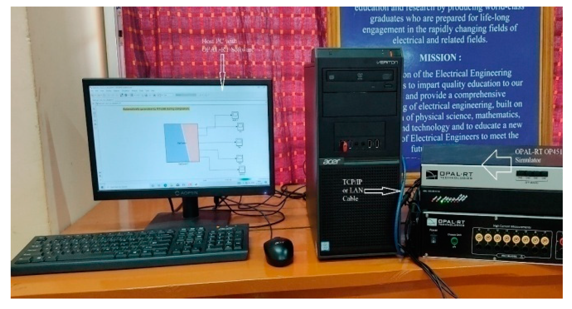
To validate the obtained simulation results using an OPAL RT 4510 real-time digital simulator.

The remainder of this paper is organized as follows. The three test systems under investigation are described in Section 2. In Section 3, the controllers (PID and TID controllers) utilized for regulation of frequency and/or voltage are discussed. In Section 4, the PSO technique is presented. In Section 5, the outcomes are discussed for all the test systems, along with validation of the obtained results. Finally, in Section 6, conclusions are presented, and future research directions are suggested.

2. System under Study

In this work, three test systems are considered for evaluation. The first and second test systems are AGC and AVR, respectively. The combined AGC and AVR problem is examined in the third test system.

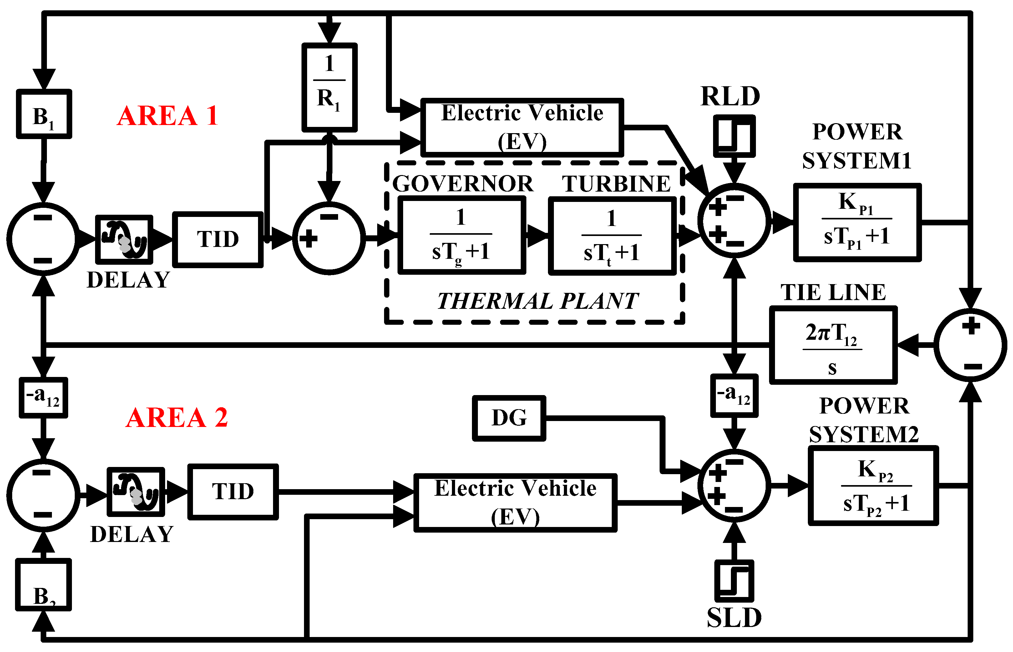
2.1. First Test System (FTS)

The FTS model is shown in Figure 1, comprising two interconnected areas. The combined electric vehicle model is considered, along with the thermal plants in area 1, with distributed generators (DGs) and EVs assumed in area 2. The DG is made up of a photovoltaic (PV) system, an aqua electrolyzer (AE), fuel cell (FC), wind turbine sources (WTS), and diesel energy generator (DEG) sources (Figure 2). The DG sources and the electric vehicles are described as follows.

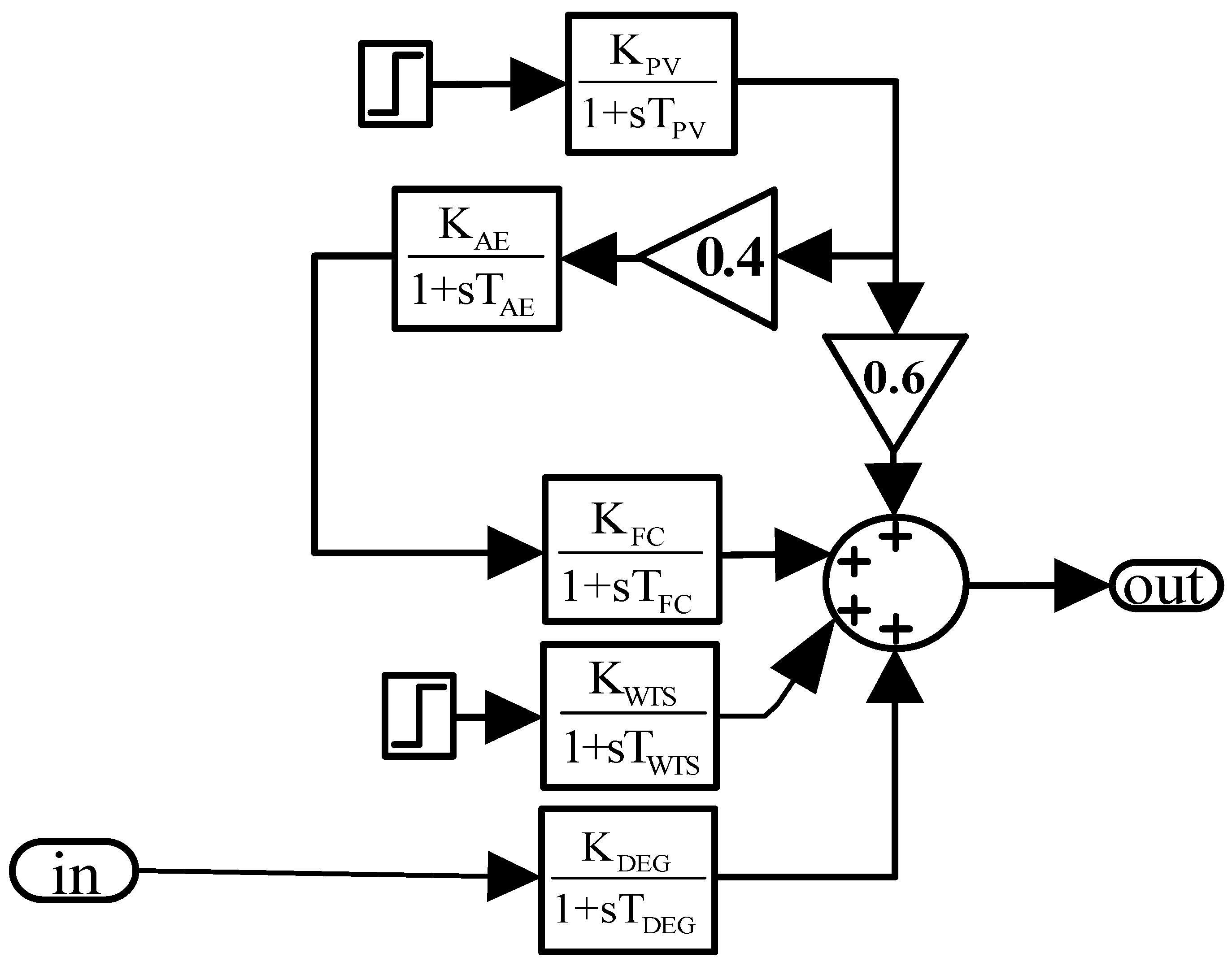
2.1.1. Photovoltaic (PV) System

A standalone PV system is an energy source that is used to provide power concurrently with other forms of energy sources. In order to transform solar energy into usable power, a PV system consists of one or more solar panels, an inverter, and other electrical and mechanical components. The DG system is configured so that 60% of the electricity generated by PV cells is delivered directly to the power grid and 40% is supplied to the aqua electrolyzer (AE). Equation (1) presents the transfer function of the PV system with corresponding gain and time constant values (K_PV and T_PV, respectively).

$${\mathrm{G}\left(\mathrm{s}\right)}_{PV}=\frac{{\mathrm{K}}_{PV}}{1+s{\mathrm{T}}_{PV}}$$

(1)

2.1.2. Aqua Electrolyzer (AE) and Fuel Cell (FC)

The aqua electrolyzer (AE) uses a portion of the PV system power (in this case, 40%) to electrolyze water to create hydrogen (H₂). The fuel cell (FC) is subsequently filled with the hydrogen generated by the AE. Equations (2) and (3) represent the transfer functions of AE and FC, respectively.

$${\mathrm{G}\left(\mathrm{s}\right)}_{AE}=\frac{{\mathrm{K}}_{AE}}{1+s{\mathrm{T}}_{AE}}$$

(2)

$${\mathrm{G}\left(\mathrm{s}\right)}_{FC}=\frac{{\mathrm{K}}_{FC}}{1+s{\mathrm{T}}_{FC}}$$

(3)

2.1.3. Wind Turbine Sources (WTS)

Kinetic energy is converted into mechanical energy by the WTS, resulting in the production of electrical energy via an induction generator. Wind power (P_WP) varies as the cube of the velocity (V_W), i.e., ${\mathrm{P}}_{\mathrm{WP}}\propto {\mathrm{V}}_{\mathrm{W}}^3$. For small signal analysis, the transfer function of WTS is given by Equation (4).

$${\mathrm{G}\left(\mathrm{s}\right)}_{WTS}=\frac{{\mathrm{K}}_{WTS}}{1+s{\mathrm{T}}_{WTS}}$$

(4)

2.1.4. Diesel Engine Generators (DEGs)

Diesel engine generators (DEGs) are also employed in the DG. The DEG relies on liquid fuels as its principal source of fuel and operates according to the principle of air compression. The transfer function of the DEG given in Equation (5).

$${\mathrm{G}\left(\mathrm{s}\right)}_{DEG}=\frac{{\mathrm{K}}_{DEG}}{1+s{\mathrm{T}}_{DEG}}$$

(5)

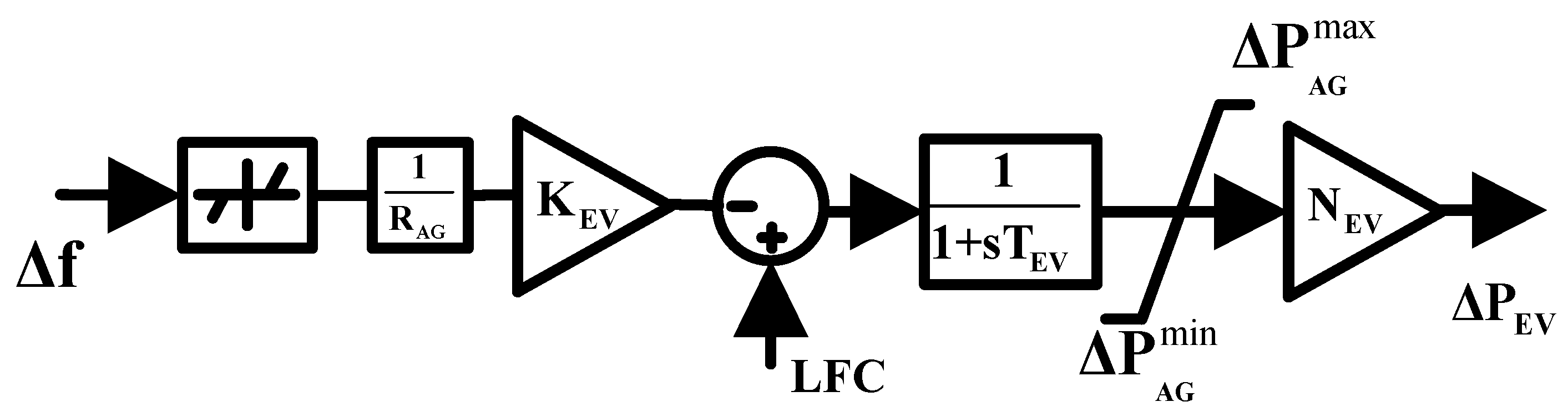
2.1.5. Electric Vehicle

Figure 3 (operating in V2G mode) depicts an aggregate model of an electric vehicle (EV) fleet comprising a battery charger, primary frequency control, and LFC. The power exchange is controlled by the battery charger. When an increased number of electric vehicles is suddenly disconnected to the grid, a poor frequency response occurs. To avoid this situation, a dead band, along with droop characteristics (R_AG), is assumed for each EV [10]. The maximum and minimum dead bands (Δf_UL and Δf_LL respectively) are taken as +10 mHz and −10 mHz, respectively. The terms ΔP_EVk, ΔP^AG_max, and ΔP^AG_min denote incremental variation in EV power and maximum and minimum power output of EV fleets, respectively. ΔP^AG_max and ΔP^AG_min are given in Equations (6) and (7), respectively. The term NEV is the total number of EVs connected to the charging station. In this study, 2000 and 1800 EVs are assumed in areas 1 and 2, respectively.

$${\mathsf{\Delta }\mathrm{P}}_{\mathrm{AG}}^{\max }=+\left[\raisebox{1ex}{${\mathsf{\Delta }\mathrm{P}}_{\mathrm{EVk}}$}\!\left/ \!\raisebox{-1ex}{${\mathrm{N}}_{\mathrm{EV}}$}\right.\right]$$

(6)

$${\mathsf{\Delta }\mathrm{P}}_{\mathrm{AG}}^{\max }=-\left[\raisebox{1ex}{${\mathsf{\Delta }\mathrm{P}}_{\mathrm{EVk}}$}\!\left/ \!\raisebox{-1ex}{${\mathrm{N}}_{\mathrm{EV}}$}\right.\right]$$

(7)

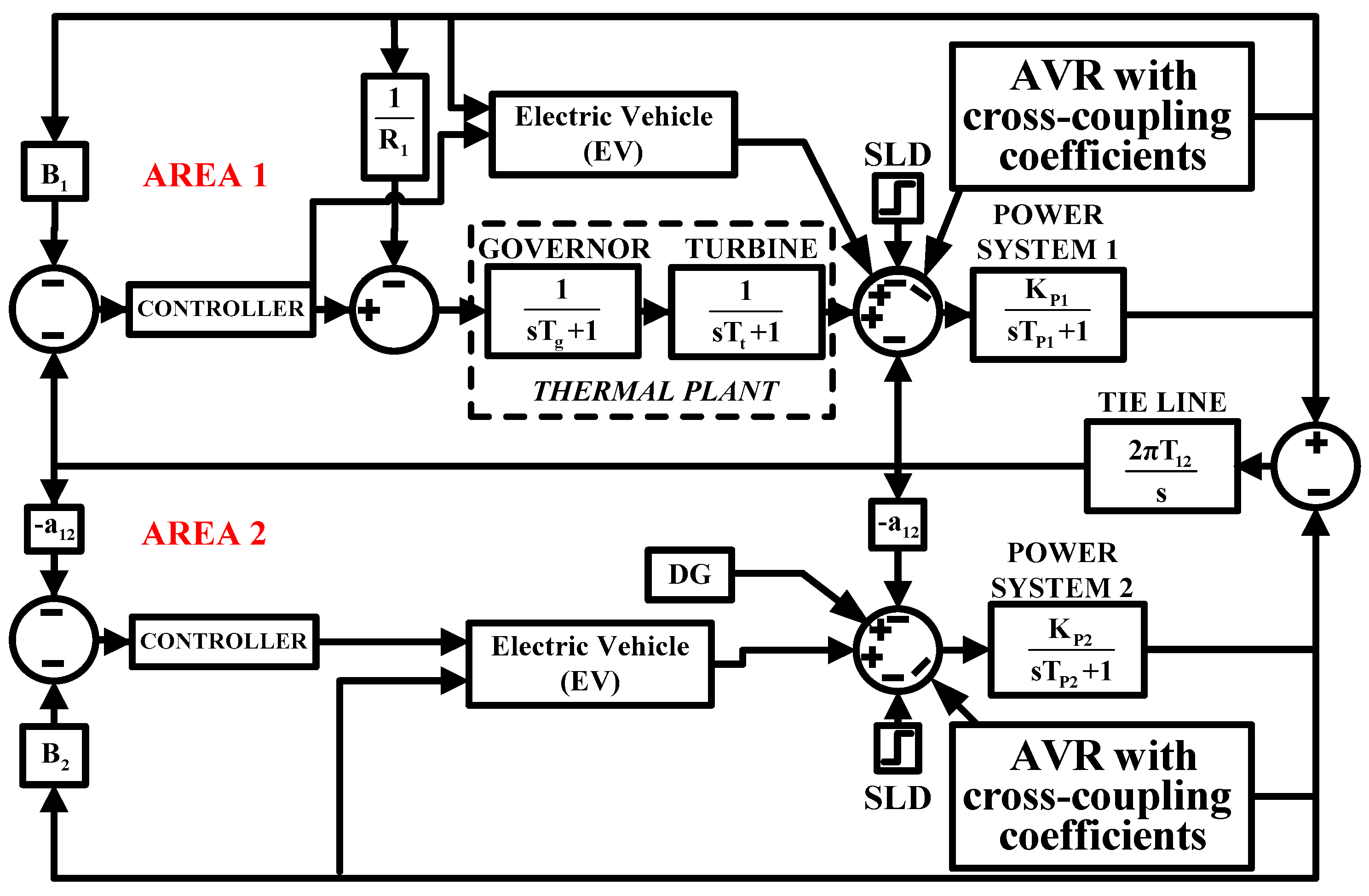
2.2. Second Test System (STS)

In the STS, only the automatic voltage regulator (AVR) problem is investigated, as shown in Figure 4.

The main function of AVR is to control the DC excitation voltage applied to the synchronous machine field circuit so that the terminal voltage remains within a reasonable range. The AVR system can also accept supplemental signals, which could enhance the stability of the dynamic rotor angle [18,19,20,21]. An amplifier, an exciter, a generator, and a sensor are the four basic parts that make up an AVR system. Exciter saturation limits and other possible causes of non-linearity are disregarded in the modelling of these components with linear equations. Transfer functions (TFs) of the various AVR components are described using Equations (8)–(11) as follows:

$$\mathrm{Amplifier}\mathrm{TF},{\mathrm{G}\left(\mathrm{s}\right)}_{Amf}=\frac{{\mathrm{K}}_{\mathrm{Ai}}}{{\mathrm{T}}_{\mathrm{Ai}}\mathrm{s}+1}$$

(8)

$$\mathrm{Exciter}\mathrm{TF},{\mathrm{G}\left(\mathrm{s}\right)}_{Exc}=\frac{{\mathrm{K}}_{\mathrm{Ei}}}{{\mathrm{T}}_{\mathrm{Ei}}\mathrm{s}+1}$$

(9)

$$\mathrm{Generator}\mathrm{field}\mathrm{TF},{\mathrm{G}\left(\mathrm{s}\right)}_{Field}=\frac{{\mathrm{K}}_{\mathrm{Fi}}}{{\mathrm{T}}_{\mathrm{Fi}}\mathrm{s}+1}$$

(10)

$$\mathrm{Sensor}\mathrm{TF},{\mathrm{G}\left(\mathrm{s}\right)}_{Sensor}=\frac{{\mathrm{K}}_{\mathrm{Si}}}{{\mathrm{T}}_{\mathrm{Si}}\mathrm{s}+1}$$

(11)

2.3. Third Test System (TTS)

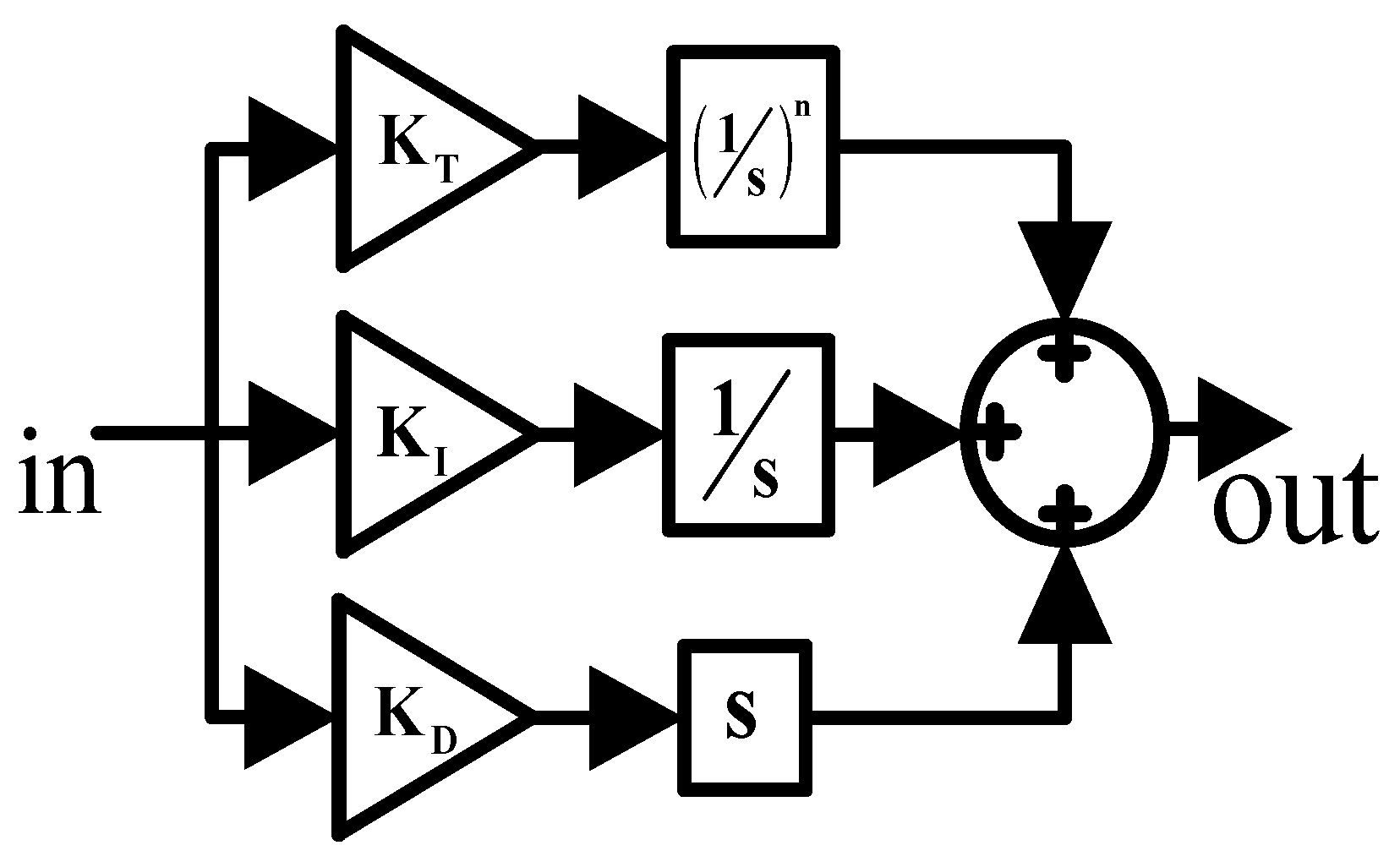
This TTS is a combination of the first and second test systems and can be used to control the frequency of the synchronous generator, tie-line powers, and terminal voltage. Figure 5 depicts a two-area interconnected model combining AGC and AVR. Figure 6 displays the cross-coupling coefficients and the AVR model that was utilized in combination with the AGC system.

For the FTS, STS, and TTS, the PID and TID controllers are assumed to perform AGC and/or AVR functions, the parameters of which are optimized using the PSO technique to determine the lowest cost value (J) using the integral squared error (ISE) method given by Equations (12)–(14). The system nominal values are depicted in

Table 1. Nominal system parameters used for investigations.

Parameter	Value
f (frequency)	60 Hz
Bi (damping constant)	0.425 pu/Hz
R (regulation)	2.4 Hz/pu
Thermal Power plant
Kg	1
Tg	0.3 s
Kt	1
Tt	0.08 s
Electric Vehicle
RAG	2.4 Hz/pu
KEV	1
TEV	1 s
Distributed Generation
KPV	1
TPV	1.8 s
KAE	1/500
TAE	0.5 s
KFC	1/100
TFC	4 s
KWTS	1
TWTS	1.5 s
KDEG	3/1000
TDEG	2 s
Power System
KPi	120
TPi	20 s
Tie Line
T12	0.0867
a12	−1
AVR
Ke	1
Te	0.4 s
Kf	0.8
Tf	1.4 s
Ka	10
Ta	0.1 s
Ks	1
Ts	0.05 s
K1	1
K2	0.1
K3	0.5
K4	1.4
Ps	0.145

.

$$J={\displaystyle \underset{0}{\overset{T}{\int }}\left(\Delta f_{area\text{-}1}{}^2+\Delta f_{area\text{-}2}{}^2+\Delta P_{tie}{}^2\right)}dt$$

(12)

$$J={\displaystyle \underset{0}{\overset{T}{\int }}\left(\Delta V_t{}^2\right)}dt$$

(13)

$$J={\displaystyle \underset{0}{\overset{T}{\int }}\left(\Delta f_{area\text{-}1}{}^2+\Delta f_{area\text{-}2}{}^2+\Delta P_{tie}{}^2+\Delta V_{t1}{}^2+\Delta V_{t2}{}^2\right)}dt$$

(14)

3. Controllers

Proportional integral derivative (PID) controllers are widely used in academia and industry, owing to its simple structure and ease of operation; a block diagram of a PID controller is depicted in Figure 7. PID controller have a poor ability to reject disturbances. In response to this issue, a fractional-order controller, i.e., a tilt-integral derivative (TID) controller is implemented in this research. The proportional gain (K_P) of a PID controller is replaced with K_T(1/s)^m in the TID controller [24], as shown in Figure 8. To optimize the parameters of these controllers, the PSO technique employed using the ISE technique given in Equations (8)–(10). The complexity associated with a TID controller compared to a PID controller is that the extra parameter, “n”, requires proper tuning.

$${\mathrm{G}\left(\mathrm{s}\right)}_{PID}{=\mathrm{K}}_P+\frac{K_I}{s}+K_{D}s$$

(15)

$${\mathrm{G}\left(\mathrm{s}\right)}_{TID}=K_T{\left(\raisebox{1ex}{$1$}\!\left/ \!\raisebox{-1ex}{$s$}\right.\right)}^m+\frac{K_I}{s}+K_D.s$$

(16)

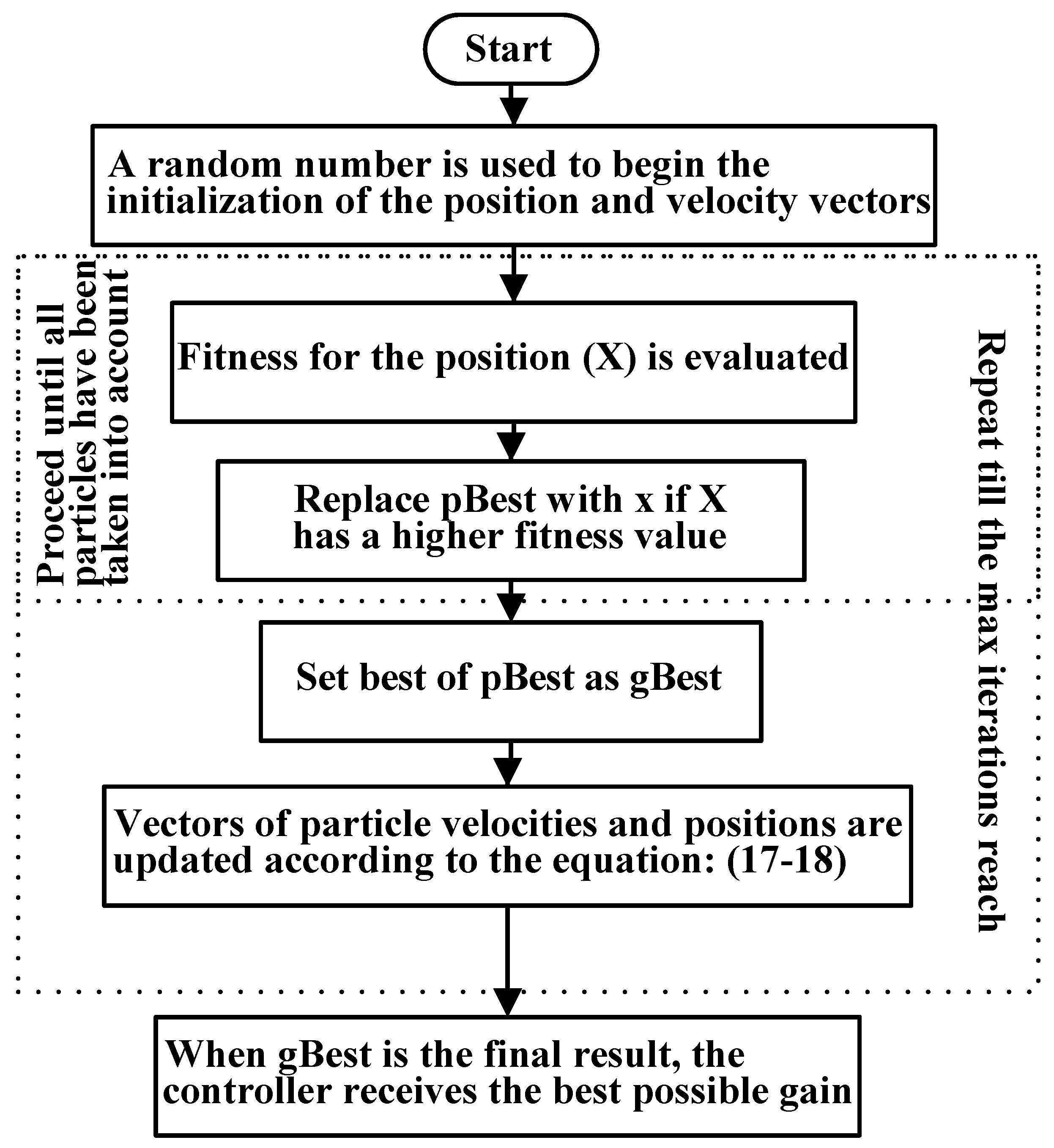
4. Particle Swarm Optimization

The particle swarm optimization (PSO) technique was developed by Kennedy and Eberhart [43] and is based on the idea of swarm intelligence observed in nature, such as in fish, birds, etc. Figure 9 shows a flow chart of the PSO technique. The velocity and position updates in PSO are given by Equations (17) and (18), respectively.

$${\mathrm{V}}_r{}^{\mathrm{m}+1}{=\mathsf{\omega }*\mathsf{\omega }}_{\mathrm{damp}}{\mathrm{V}}_r{}^{\mathrm{m}}+{\mathrm{a}}_1{h}_1\times \left({\mathrm{pBest}}_r^{\mathrm{m}}-{\mathrm{X}}_j{}^{\mathrm{m}}\right)+{\mathrm{a}}_2{h}_2\times \left({\mathrm{pBest}}_r^{\mathrm{m}}-{\mathrm{P}}_r{}^{\mathrm{m}}\right)$$

(17)

$$P^{m+1}=P_r+V^{m+1}$$

(18)

where i = 1, 2,3,…… Z, where Z is the total number of particles, and t is the iteration number currently in use. Furthermore,

c₁ and c₂ are the acceleration constants;

The integer values of r₁ and r₂ are completely random and fall between 0 and 1;

V_r^t is the velocity of particle i for the t^th iteration;

ω is the inertia weight;

ω_damp is the damping factor;

X_i^t is the position of particle i in the t^th iteration;

pBest^t_i is the previous best location of particle i; and

gBest^t_i is the global best location of the particles.

The PSO technique is applied to tune the considered TID and PID controller parameters. The following PSO parameters were taken into consideration: population size, Z = 10; iterations, iter = 100; inertia weight, ω = 1; learning rates, c1 = c2 = 1.496; and damping factor, ω_damp = 0.729.

5. Results and Discussion

Three test systems are considered for study, namely AGC, AVR, and the combination of AGC and AVR. The performance of the PID and TID controllers was evaluated using the above-described test systems optimized using the PSO technique. Multiple case studies were conducted, considering factors such as increased load demand, randomized load demand, non-linearities, delays, etc., to extract the performance of the controllers.

5.1. First Test System (AGC)

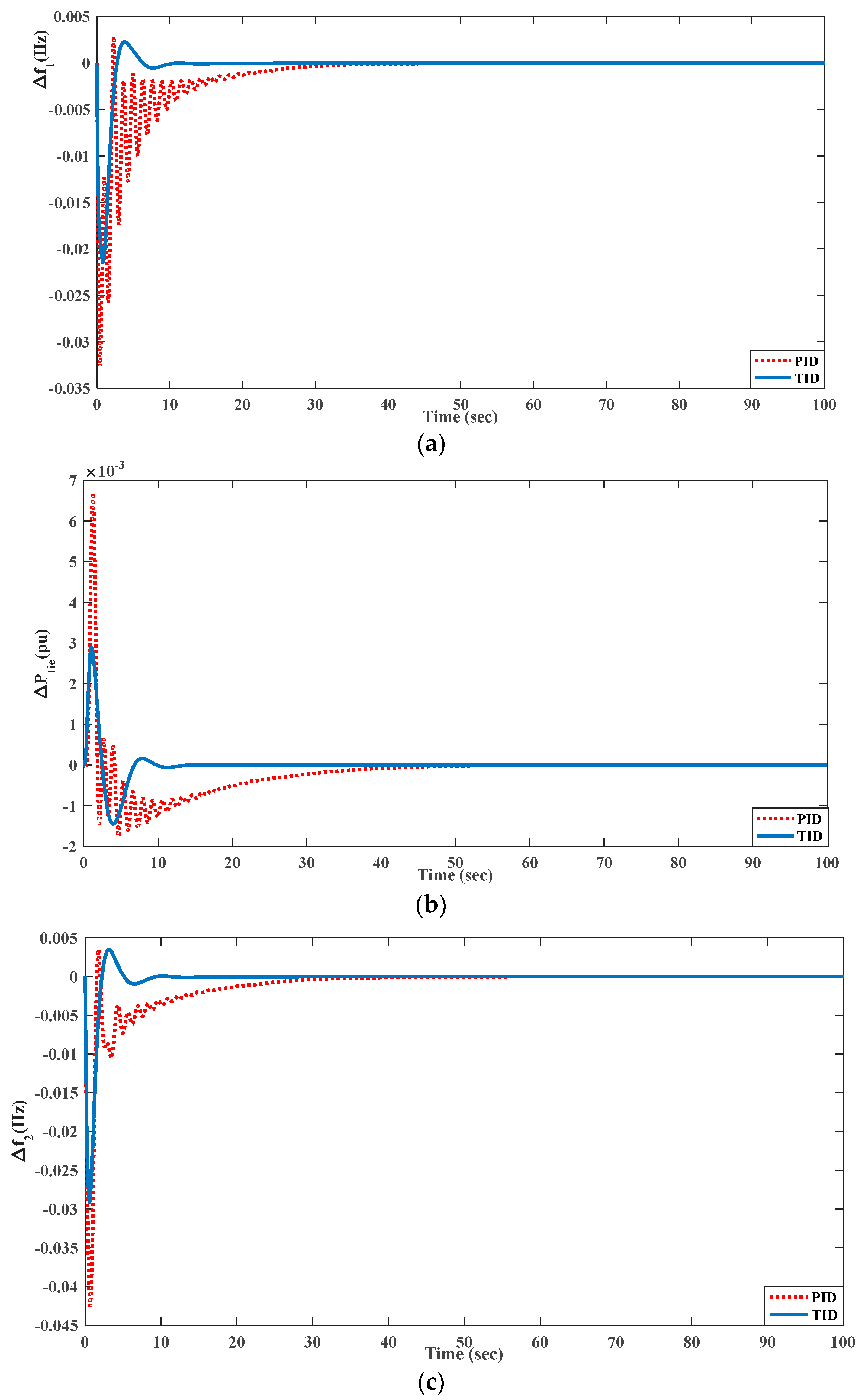
5.1.1. With 1% SLD in Both Areas

The system under examination in this case is a two-area connected system. Area 1 has both thermal and electric vehicles, and area 2 connects distributed generation and electric vehicles. The PID and TID controllers are used to suppress the system dynamics, the control variables of which are optimized using the PSO technique with a 1% magnitude of step load disturbance (SLD). The corresponding optimized values are listed in

Table 2. PID parameter values for 1% SLP.

Parameter	KP	KI	KD
Area 1	0.7611	0.544	0.2415
Area 2	0.711	0.3576	0.3367

and

Table 3. TID parameter values for 1% SLP.

Parameter	KT	n	KI	KD
Area 1	0.9563	3.14	0.7429	0.9999
Area 2	0.9653	4.0823	0.8799	0.984

. The comparative dynamic responses of Δf₁, Δf₂, and ΔP_tie are shown in Figure 10 for PID and TID controllers. The dynamic measures of these responses, peak values of overshoots, undershoots, and settling durations are shown in

Table 4. Dynamic measures with PID and TID controllers.

	Parameter	∆f1 (Hz)	∆f2 (Hz)	∆Ptie (pu)
PID	Peak Overshoot (in 10^(−3))	3.48	3.24	NIL
	Peak Undershoot (in 10^(−3))	11.08	2.491	2.8
	Settling Time(s)	19.74	18.2	20.3
TID	Peak Overshoot (in 10^(−3))	1.294	1.387	NIL
	Peak Undershoot (in 10^(−3))	5.902	0.54	2.006
	Settling Time(s)	10.4	6.8	12.5

. Figure 10 and Table 4 clearly demonstrates that the TID controller enhances system dynamics compared to the PID controller.

5.1.2. Comparative Performance of GA, ACO, and PSO

The performance of the PSO-based TID controller is tested against the genetic algorithm (GA) and ant colony optimization (ACO) when tuned with same controller. The convergence curves obtained for these algorithms with the TID controller are plotted in Figure 11, which shows the superiority of proposed PSO–TID controller. The cost values obtained with ACO and GA are 0.00127 and 0.018, respectively which are greater than the cost corresponding to PSO (0.000289).

5.1.3. With 2% SLD in Both Areas

The performance of the PID and TID controllers is evaluated here for a higher magnitude of disturbance, i.e., 2% SLD in both the areas with the control variables mentioned in Table 2 and Table 3. According to the dynamics plotted in Figure 12, the TID controller clearly outperforms the PID controller in terms of multiple dynamic metrics.

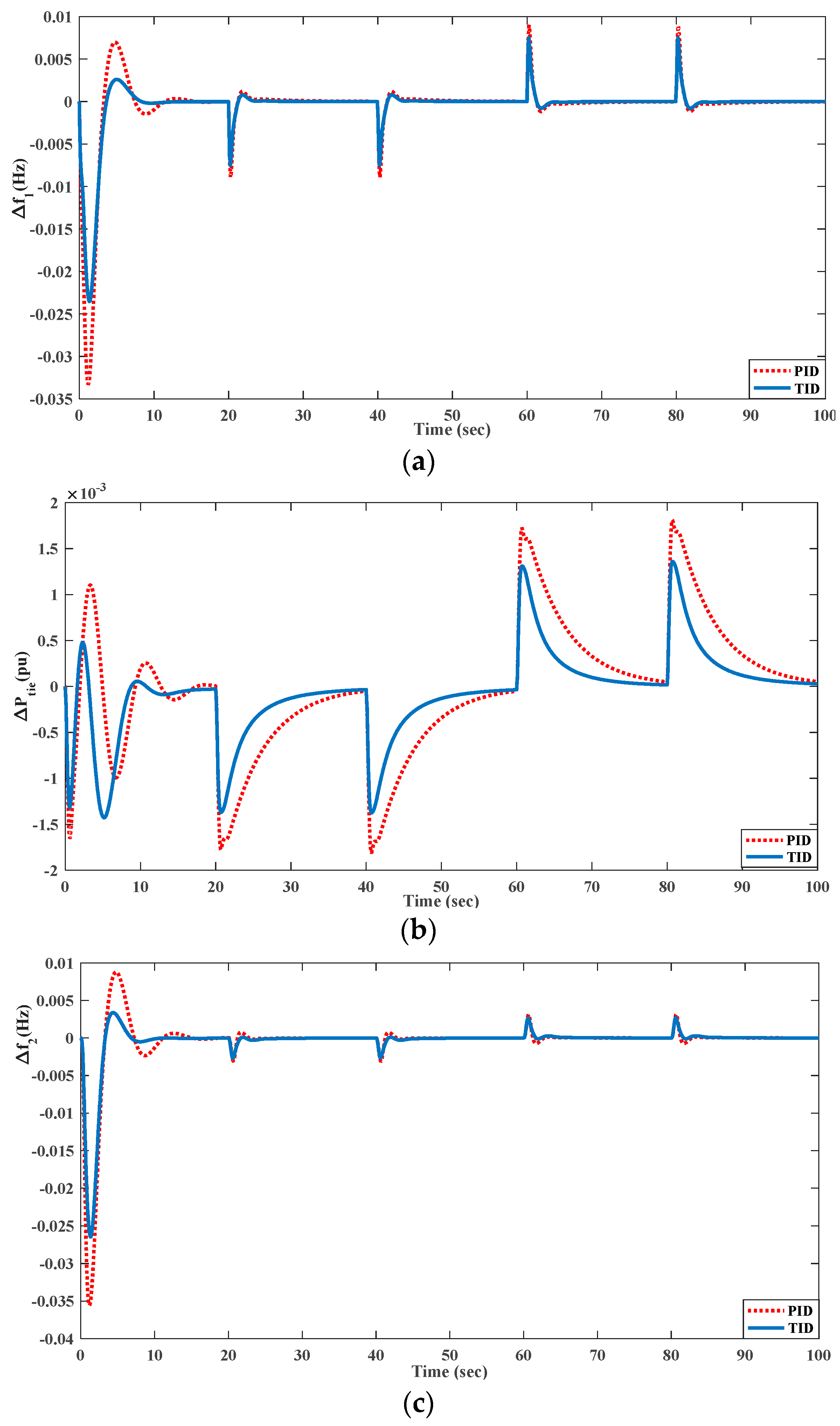
5.1.4. Randomized Load Pattern

As the load on the power system varies continuously, it is worthwhile to study the performance of the controller with random loads. To this end, a randomized load pattern (RLP), as shown in Figure 13, is assumed, and the performance of the PID and TID controllers is evaluated using the 1% SLD optimized values (Table 2 and Table 3). The results reveal enhanced dynamics of the TID controller relative to the PID controller in terms of dynamic measures, such as oscillation magnitudes and peak over- and undershoots (Figure 14).

5.1.5. With Non-Linearities

This study examines the effect of non-linearities, such as the reheat turbine (RT), generation rate constraints (GRCs), and governor dead band (GDB), on system dynamics in the presence of PID and TID controllers. The PSO technique is used to optimized the control parameters, and corresponding responses are shown in Figure 15. The optimized PID and TID controller values are given in

Table 5. PID controller parameters with non-linearities.

Parameter	KP	KI	KD
Area 1	0.0187	0.2536	0.6999
Area 2	0.1962	0.1999	0.5905

and

Table 6. TID controller parameters with non-linearities.

Parameters	KT	n	KI	KD
Area 1	0.5977	4.3453	0.6986	0.9999
Area 2	0.9984	2.1517	0.8569	0.9618

, respectively. The PID controller is unable to handle the system dynamics with RT, GRC, and GDB non-linearities, whereas the TID controller provides satisfactory performance, as shown in

Table 7. Comparison of dynamic measures with PID and TID controllers.

	Parameter	∆f1 (Hz)	∆f2 (Hz)	∆Ptie (pu)
PID	Peak Overshoot (in 10^(−3))	4.2	2.65	1.4
	Peak Undershoot (in 10^(−3))	15.24	8.56	5.64
	Settling Time(s)	-	-	-
TID	Peak Overshoot (in 10^(−3))	1.4	1.116	1.8
	Peak Undershoot (in 10^(−3))	8.45	3.6	2.98
	Settling Time(s)	15.1	17.3	15.3

.

5.1.6. With Time Delays

Here, it is assumed that the control signal travels from the remote point to the control center with a delay of 0.2 and 0.4 s. With these delays, the PSO approach is used to obtain the control parameters of the PID and TID controllers (

Table 8. PID controller parameters with a 0.2 s delay.

Parameter	KP	KI	KD
Area 1	0.5854	0.4321	0.6764
Area 2	0.6530	0.7517	0.8960

,

Table 9. TID controller parameters with a 0.2 s delay.

Parameter	KT	n	KI	KD
Area 1	0.5773	1.9058	0.4240	0.4195
Area 2	0.9999	1.3026	0.5228	0.2710

,

Table 10. PID controller parameters with a 0.4 delay.

Parameter	KP	KI	KD
Area 1	0.0477	0.6158	0.1237
Area 2	0.1741	0.5329	0.6851

and

Table 11. TID controller parameters with a 0.4 s delay.

Parameter	KT	n	KI	KD
Area 1	0.6562	1.1248	0.0171	0.156
Area 2	0.7948	2.764	0.7713	0.2199

), and dynamics are plotted in Figure 16 and Figure 17. The PID controller can only tolerate the delay effect up to 0.2 s, after which it provides unstable system dynamics. On the other hand, the TID controller achieves stabilized performance even with a delay of 0.4 s. Hence, TID controllers are preferred over PID controllers with larger system delays.

5.2. Second Test System (AVR)

5.2.1. Time Domain Analysis of AVR

Here, studies related to AVR are performed using PID and TID controllers, the parameters of which are obtained through the PSO technique (

Table 12. Optimized PID controller parameters for AVR.

Parameter	KP	KI	KD
AVR	0.7974	0.9999	0.8416

and

Table 13. Optimized TID controller parameters for AVR.

Parameter	KT	n	KI	KD
AVR	0.9103	3.11	0.2531	0.4903

). The dynamics of outputs corresponding to AVR, namely V_t1 and V_t2, are plotted in Figure 18. The TID controller shows superior dynamics measures, such as settling duration, as well as peak over- and undershoots (

Table 14. Comparative dynamic measures with PID and TID controllers.

	Parameter	Vt (pu)
PID	Peak Overshoot	1.346
	Peak Undershoot	NIL
	Settling Time(s)	11.3
TID	Peak Overshoot	1.23
	Peak Undershoot	NIL
	Settling Time(s)	5.1

).

5.2.2. Frequency Domain Analysis through Bode Plot

Here, the AVR system is analyzed with help of a Bode plot using PID and TID controllers. The transfer functions of AVR are given by Equations (19) and (20).

$${\mathrm{G}\left(\mathrm{s}\right)}_{PID}^{AVR}=\frac{{\mathrm{G}\left(\mathrm{s}\right)}_{PID}·{\mathrm{G}\left(\mathrm{s}\right)}_{Amf}·{\mathrm{G}\left(\mathrm{s}\right)}_{Exc}·{\mathrm{G}\left(\mathrm{s}\right)}_{Field}}{1+{\mathrm{G}\left(\mathrm{s}\right)}_{PID}·{\mathrm{G}\left(\mathrm{s}\right)}_{Amf}·{\mathrm{G}\left(\mathrm{s}\right)}_{Exc}·{\mathrm{G}\left(\mathrm{s}\right)}_{Field}}$$

(19)

$${\mathrm{G}\left(\mathrm{s}\right)}_{TID}^{AVR}=\frac{{\mathrm{G}\left(\mathrm{s}\right)}_{TID}·{\mathrm{G}\left(\mathrm{s}\right)}_{Amf}·{\mathrm{G}\left(\mathrm{s}\right)}_{Exc}·{\mathrm{G}\left(\mathrm{s}\right)}_{Field}}{1+{\mathrm{G}\left(\mathrm{s}\right)}_{TID}·{\mathrm{G}\left(\mathrm{s}\right)}_{Amf}·{\mathrm{G}\left(\mathrm{s}\right)}_{Exc}·{\mathrm{G}\left(\mathrm{s}\right)}_{Field}}$$

(20)

Bode plots provide information on the stability of the system via frequency response of a control system, with two plots, namely a magnitude plot and phase plot. A brief discussion of these plots is provided below.

Gain margin is the amount of gain that can be decreased or increased without causing the system to become unstable. The higher the gain margin, the greater the stability of the system. The standard unit of measurement for gain margin is dB.

Phase margin is the maximum value of the phase angle that can be decreased or increased without causing the system to become unstable. The larger the phase margin, the higher the degree of system stability. It is defined as the magnitude of the phase angle and is measured in degrees.

The Bode plots (magnitude and frequency) are shown in Figure 19 with the optimum values listed in Table 12 and Table 13 using the AVR system transfer functions corresponding to the PID and TID controllers. The TID controller achieves a higher value for both the gain margin (6 dB) and the phase margin (14.2 degrees) compared to the PID controller (1.16 dB and 5.29 degrees, respectively), indicating the superiority of the former in terms of stability.

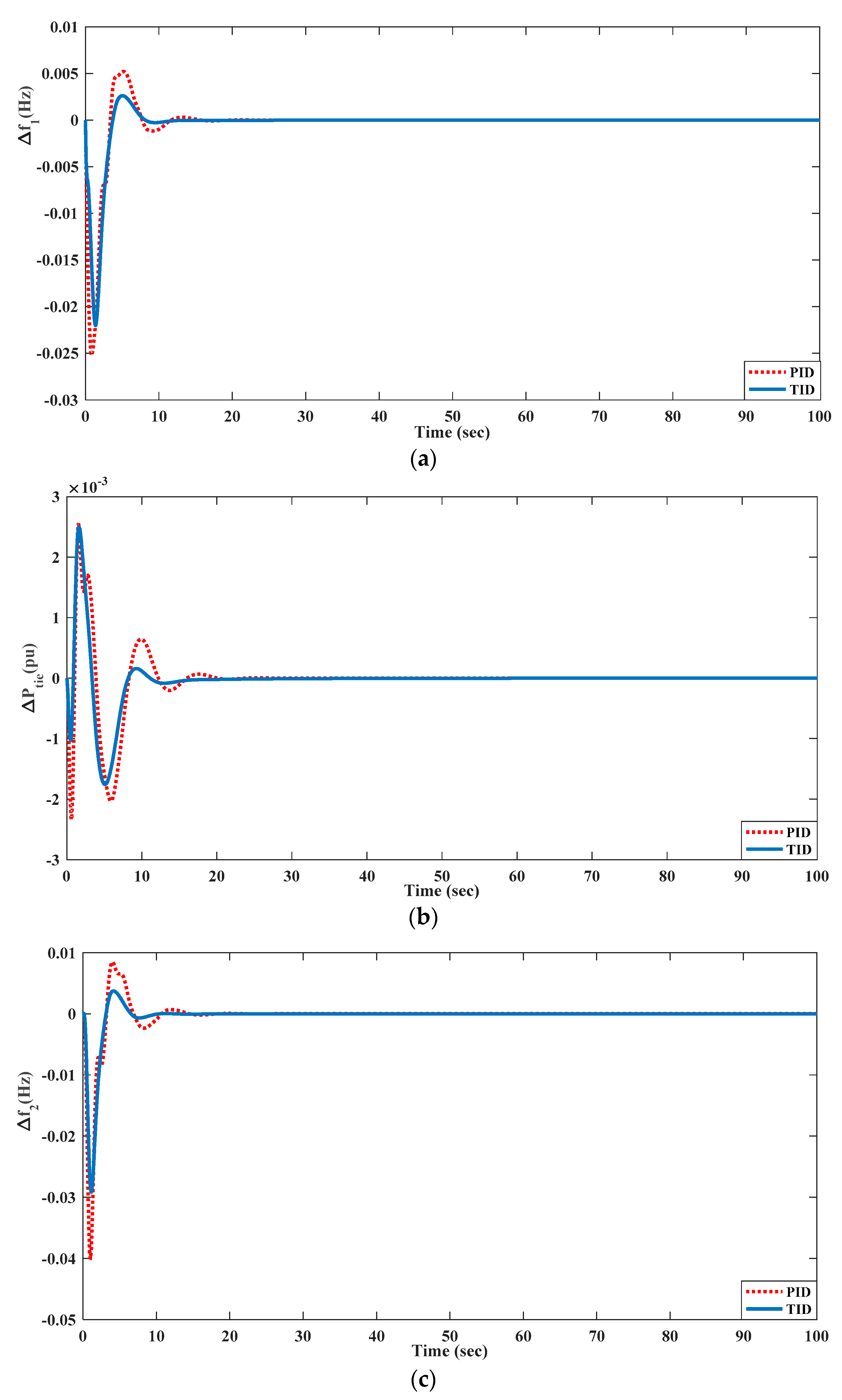
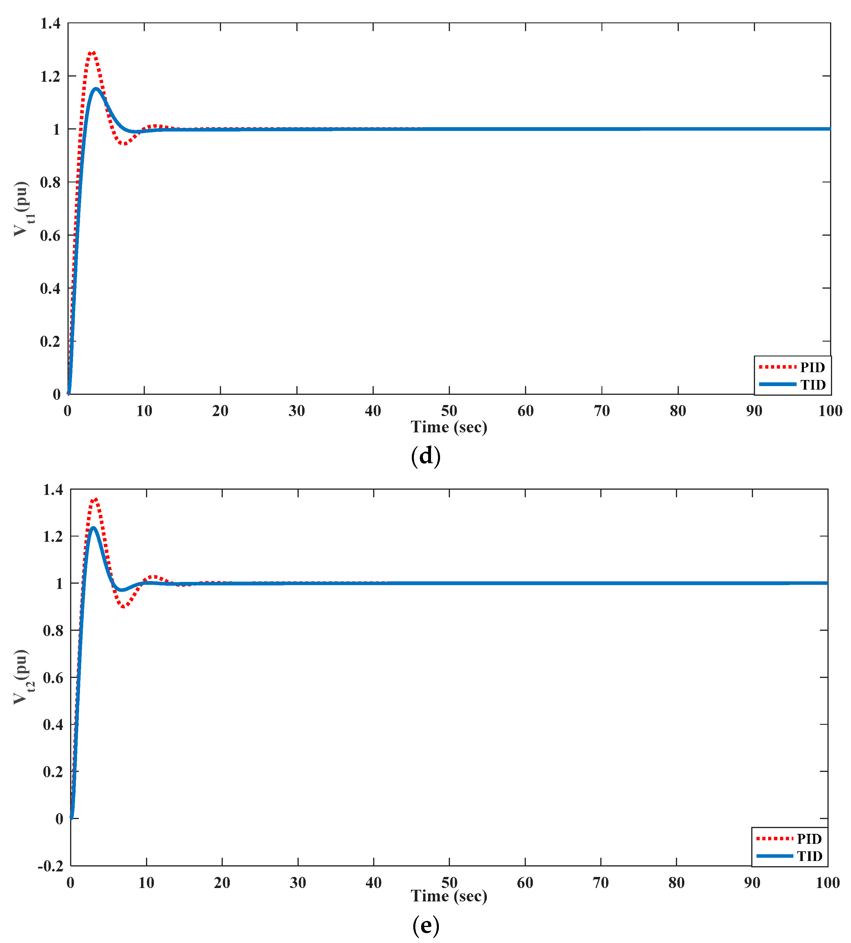
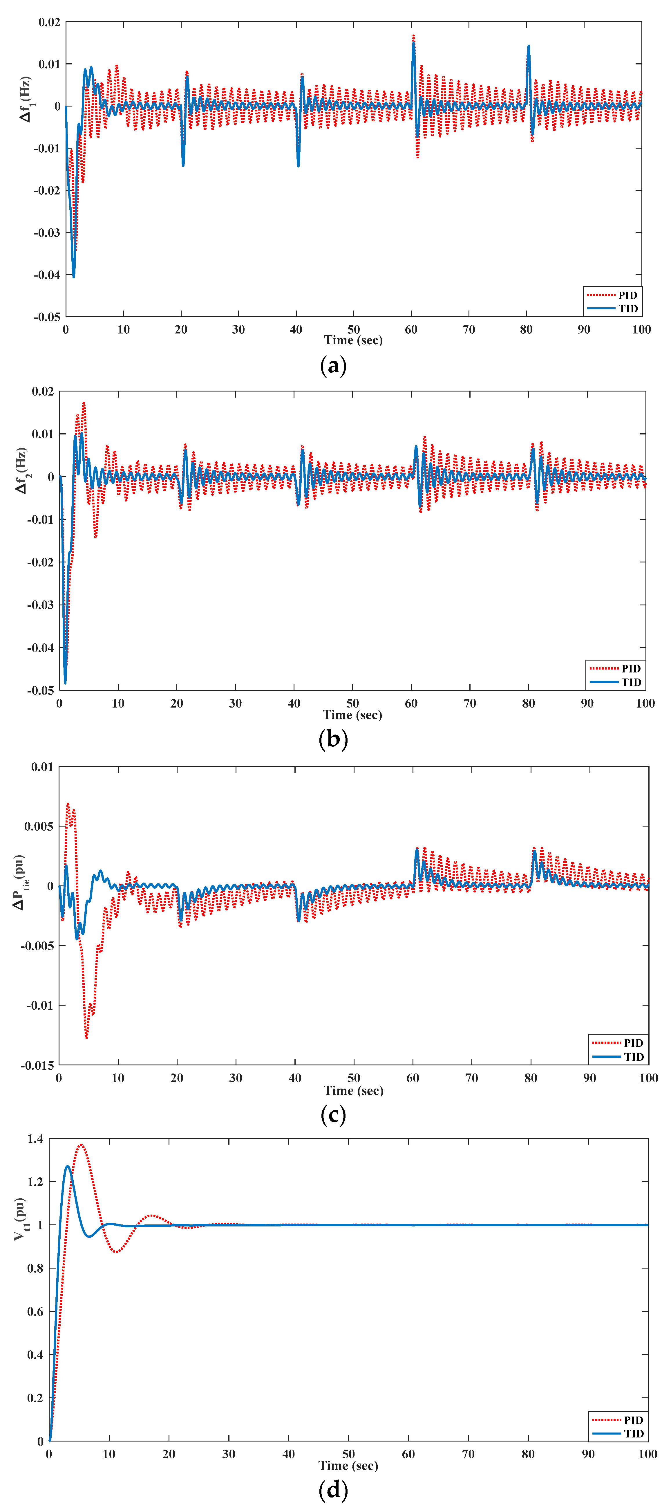
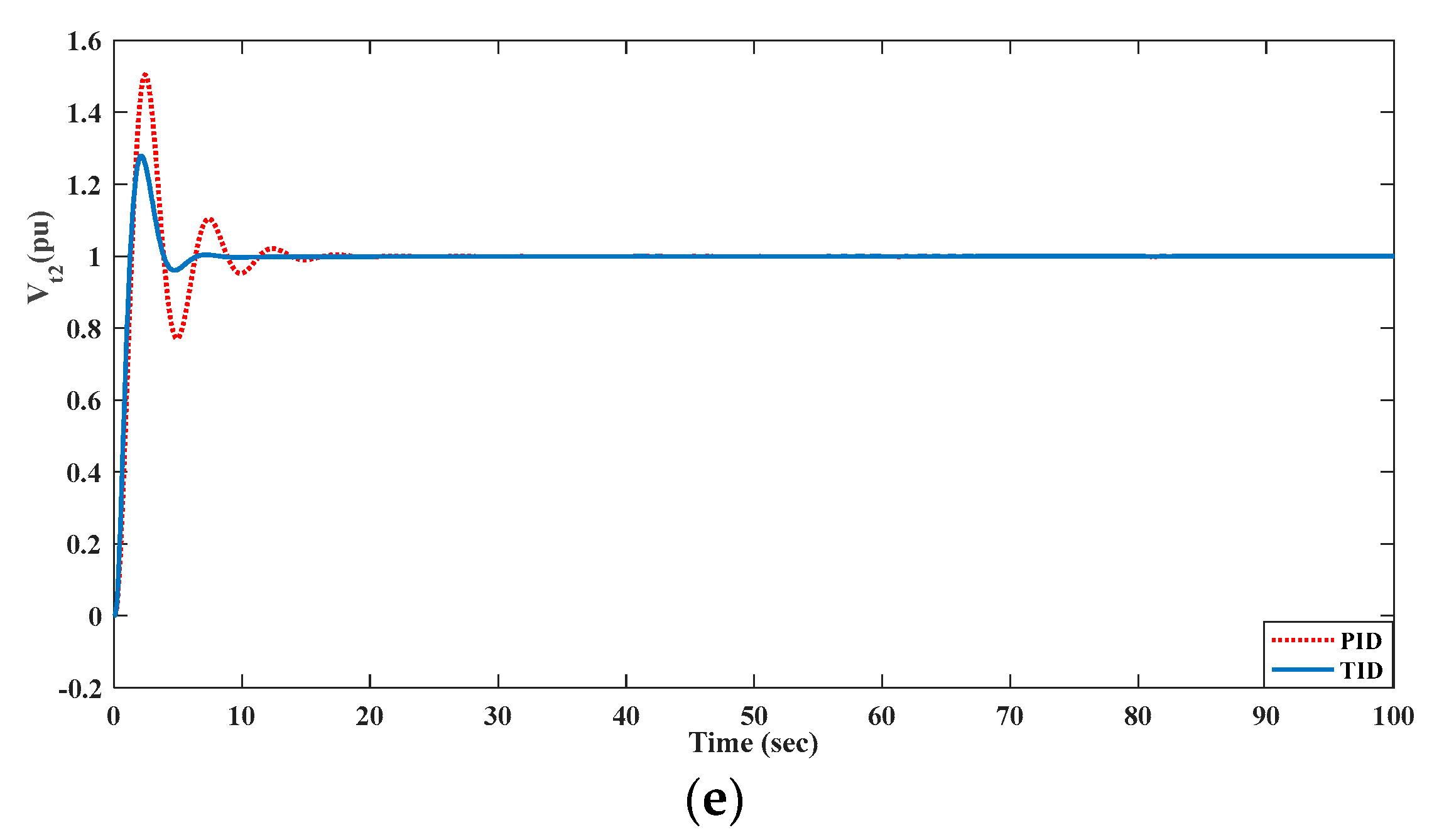
5.3. Third Test System (Combination of AGC and AVR)

5.3.1. With Step Load Disturbance

Here, a two-area interconnected combined control of frequency and voltage control problem is investigated, the model of which is shown in Figure 5. In this case, the PID and TID control parameters are tuned with the PSO technique, with optimum values depicted in

Table 15. PID parameters for the combined AGC and AVR system.

Parameter	KP	KI	KD
Area 1	0.2589	0.65649	0.6239
Area 2	0.0218	0.2297	0.485
AVR 1	0.7682	0.8001	0.7957
AVR 2	0.7723	0.998	0.9827

and

Table 16. TID parameters for the combined AGC and AVR system.

Parameter	KT	n	KI	KD
Area 1	0.9552	3.0699	0.8319	0.9255
Area 2	0.9399	2.909	0.8348	0.9453
AVR 1	0.8776	3.777	0.268	0.9696
AVR 2	0.957	2.999	0.3594	0.8492

, respectively. With these parameters, the dynamics of Δf₁, Δf₂, ΔP_tie, V_t1, and V_t2 are determined and compared between PID and TID controllers (Figure 20), with corresponding measures noted in Table 15 and Table 16, indicating the superiority of the TID controller over the PID controller in terms of various dynamic measures, as evidenced by the dynamic measures listed in

Table 17. Comparison of AGC dynamics for PID and TID controllers.

	Parameter	∆f1 (Hz)	∆f2 (Hz)	∆Ptie (pu)
PID	Peak Overshoot (in 10^(−3))	7	8.77	1.1
	Peak Undershoot (in 10^(−3))	33.3	35.5	1.654
	Settling Time(s)	16.8	16.3	22.7
TID	Peak Overshoot (in 10^(−3))	2.6	3.37	0.478
	Peak Undershoot (in 10^(−3))	23.5	26.45	1.43
	Settling Time(s)	10.1	7.2	19.6

and

Table 18. Comparison of AVR dynamics for PID and TID controllers.

	Parameter	Vt1 (pu)	Vt2 (pu)
PID	Peak Overshoot	1.293	1.36
	Peak Undershoot	NIL	NIL
	Settling Time(s)	12.43	15.1
TID	Peak Overshoot	1.151	1.235
	Peak Undershoot	NIL	NIL
	Settling Time(s)	8.51	7.88

.

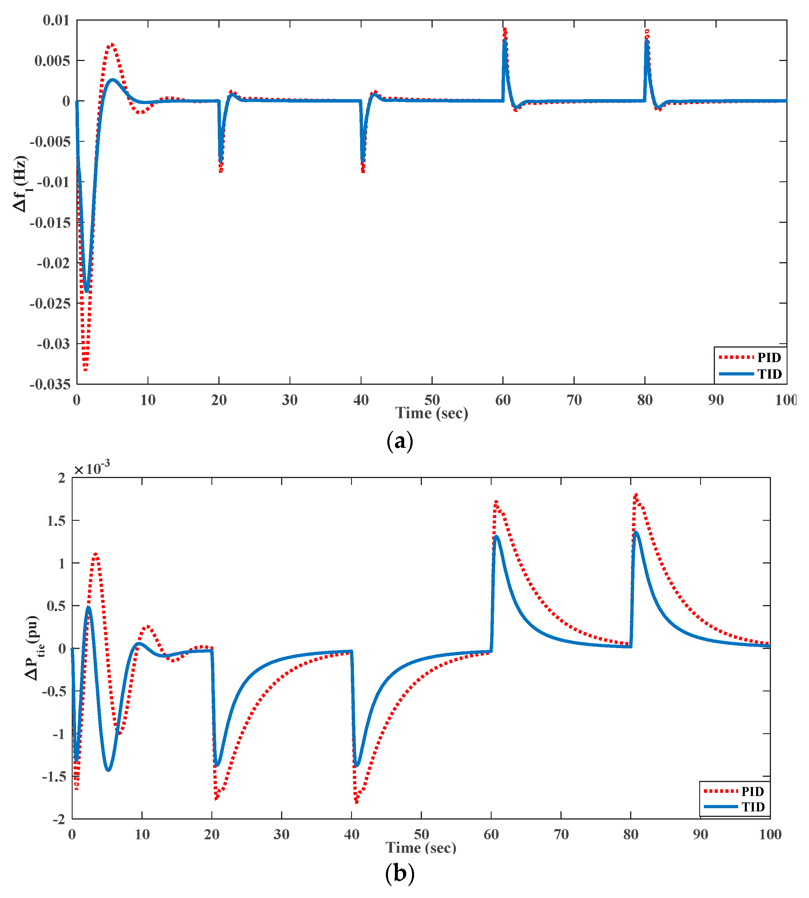
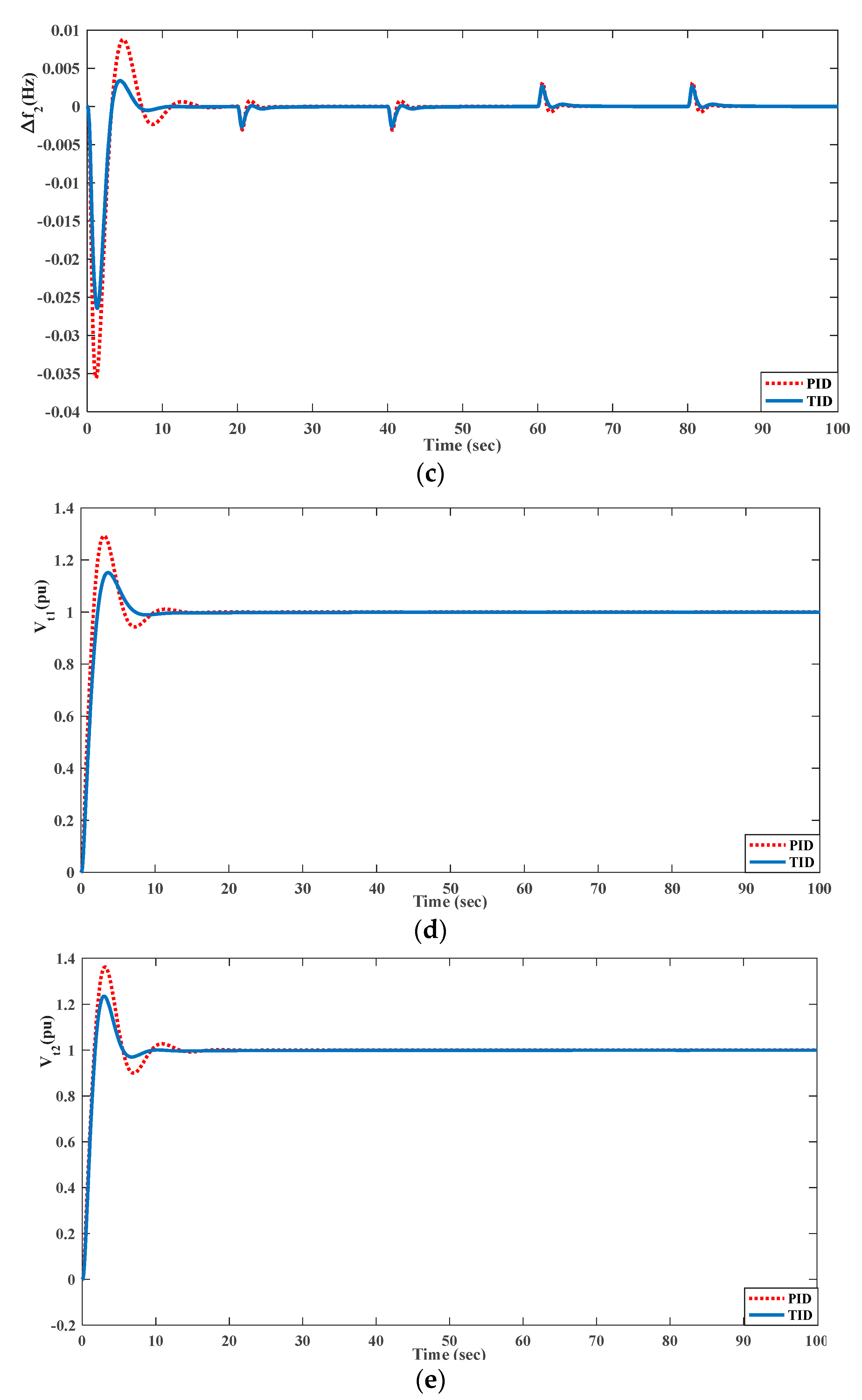
5.3.2. Randomized Load Pattern

The combined AGC and AVR problem was also tested against RLP, as shown in Figure 13. With RLP, the PID and TID controller performance is evaluated with the optimized values presented in Section 5.3.1 (Table 15 and Table 16). The TID controller achieves superior dynamic responses relative to those achieved with the PID controller (Figure 21).

5.3.3. Combined Effect of Non-Linearities and Time Delays against RLP

The combined AGC and AVR system with non-linearities (GDB, GRC, and RT) was tested to compare the performances of PID and TID controllers with a time delay (0.2 s) against RLP (Figure 13). The PSO-optimized PID and TID controller parameters are depicted in

Table 19. PID parameters for the combined AGC and AVR system with RLD, all non-linearities, and a 0.2 s delay.

Parameter	KP	KI	KD
Area 1	0.9260	0.8404	0.4653
Area 2	0.2083	0.5591	0.4756
AVR 1	0.3962	0.3576	0.7463
AVR 2	0.3156	0.6342	0.0663

and

Table 20. TID parameters for the combined AGC and AVR system with RLD, all non-linearities, and a 0.2 s delay.

Parameter	KT	n	KI	KD
Area 1	0.0743	1.087	0.82285	0.9255
Area 2	0.9567	3.6834	0.4888	0.9961
AVR 1	0.7247	2.5301	0.3014	0.6471
AVR 2	0.9999	3.6129	0.5001	0.4756

, respectively, with system dynamics plotted and compared in Figure 22. With the TID controller, the oscillations and peak over- and undershoots are lower than those observed with the PID controller.

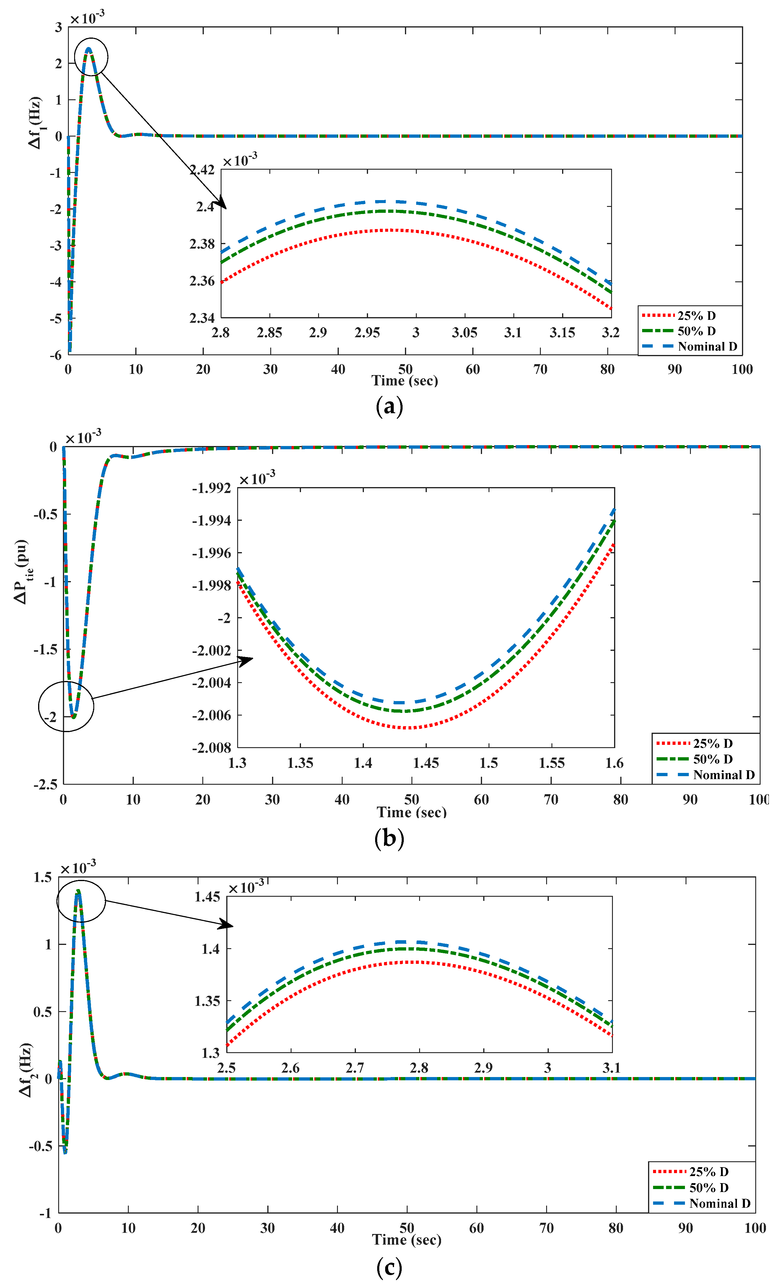
5.4. Insensitivity of the TID Controller

5.4.1. Insensitivity to Variation in D

For the AGC system shown in Figure 1, the frequency-dependent damping constant (D) is modified significantly, and its impact on system performance is studied. The value of D is altered by 25% and 50% relative to nominal values. Figure 23 shows that even if the D values are changed, the responses do not change at all, demonstrating that TID controller variables are resistant to changes in D.

5.4.2. Insensitivity to Variation in Time Constants of the AVR System

Here, the TID controller parameters of the third test system shown in Table 15 and Table 16 are tested for robustness by changing the AVR time constants (time constants of exciter, amplifier, generator field, and sensor) in both areas by ±30% of their nominal values shown in Table 1. The dynamics of various responses are plotted with changed and nominal values of time constants of the AVR system in Figure 24. In both the cases (changed and unchanged), the dynamics are similar, indicating the robustness of optimum TID controller parameters in response to considerable variations in the time constants of the AVR system.

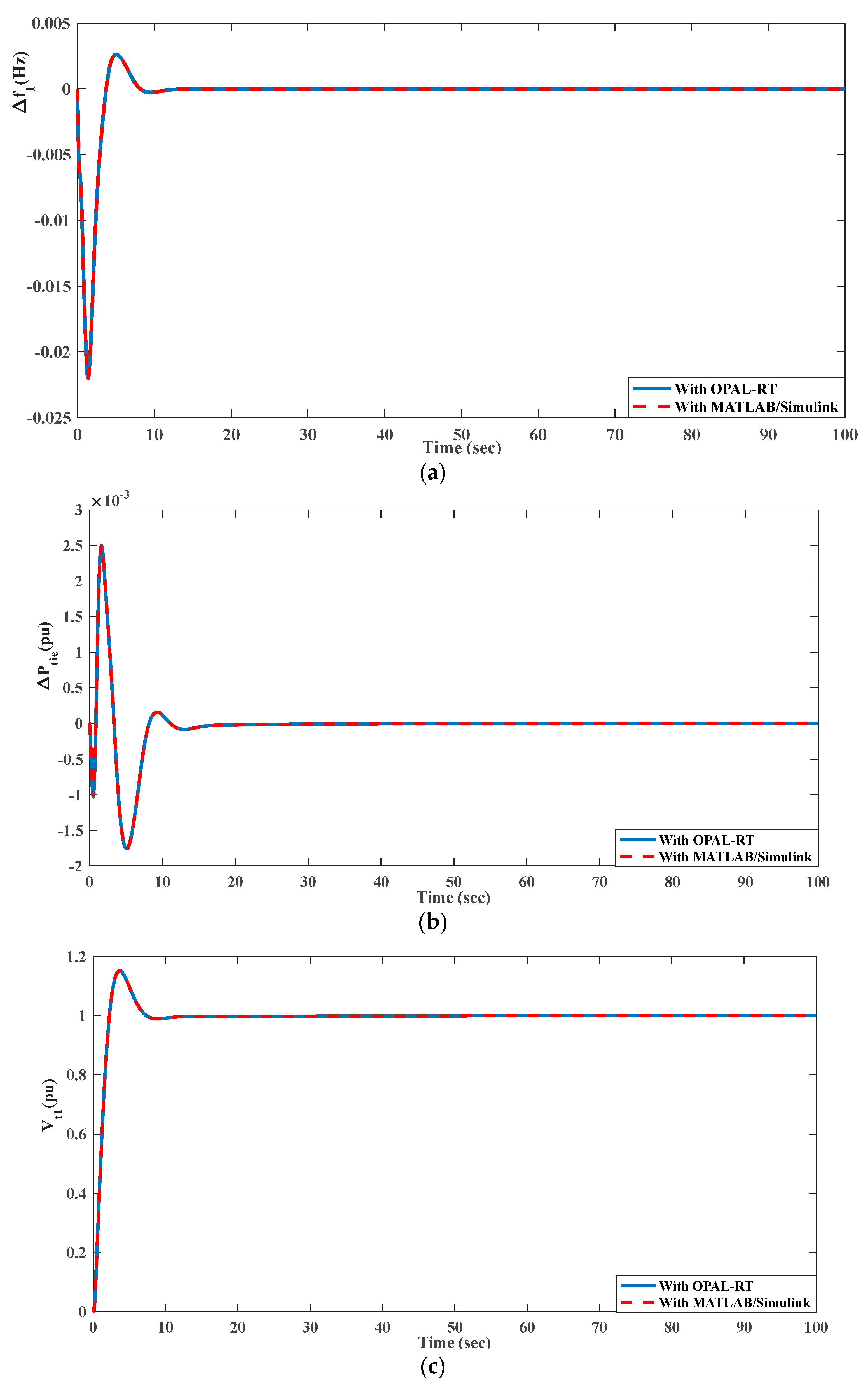
5.5. Validation of Results

The proposed combined automatic voltage regulator (AVR) and automatic generator control (AGC) system for two-area power plants is verified using an OPAL-RT OP4510 real-time digital simulator. The OP4510 uses the most up-to-date Intel generation Xeon 4-core processors and a robust Xilinx Kintex-7 FPGA platform. It is capable of performing real-time parallel processing; therefore, the outcomes are similar to those obtained with the hardware [23,29]. The OPAL-RT OP4510 laboratory setup includes a host PC running RT-Lab software, I/O ports, a TCP/IP connection, and the real-time digital simulator shown in Figure 25. In order to validate the proposed combined ALFC and AVR control problem, the system model is first constructed on the MATLAB/Simulink R2018 platform and fed to OPAL-RT OP4510 through RT-LAB software, which integrates MATLAB and runs in real time with multiple cores. The OPAL-RT platform findings (indicated in blue) are compared with the simulation results obtained in Section 5.3.1. Figure 26 shows that the findings obtained with MATLAB/Simulink and OPAL-RT OP4510 are almost identical, confirming the validity of the obtained results.

6. Conclusions

In the present study, the effectiveness of a TID controller was explored in comparison with a commonly employed PID controller to address the AGC and/or AVR problem in regulating frequency and/or voltage. The PID and TID controller parameters were optimized using the PSO technique. The TID controller outperformed the PID controller in terms of various dynamics measures, such as settling time, as well as peak overshoots and undershoots, in case studies with 1% SLD, 2% SLD, a randomized load pattern, non-linearities (GDB, GRC, and RT), etc. PSO achieved superior performance compared to genetic algorithm and ant colony optimization techniques. Investigations revealed that the PID controller is unable to provide stabilized oscillations with a delay of 0.4 s, whereas the TID controller achieved satisfactory performance. The PSO-tuned TID controller parameters are insensitive to wide variations in damping factor and time constants of the AVR system. The obtained simulation results were validated with the real-time OPAL-RT 4510 simulation platform.

7. Future Recommendations

The performance of PS-tuned TID controllers can be tested on the deregulated AGC or combined AGC-AVR problem with respect to the regulation of various system dynamics. The cascade combination of TID controllers can be tested to address the AGC and/or AVR problem to improve the regulation of system dynamics. A combination of fuzzy-based TID controllers can be designed to regulate frequency and/or voltage in an interconnected power system. The proposed optimization technique, which provides competitive global optimum results, can be applied to design the controllers mentioned above. The frequency-dependent factor, i.e., load-damping factor variation can be studied in the presence of a cascade TID or fuzzy-based TID controllers with electric vehicles [47,48] and/or wind turbine generators [49].

References

1. Kalyan, C.N.S.; Goud, B.S.; Reddy, C.R.; Bajaj, M.; Sharma, N.K.; Alhelou, H.H.; Siano, P.; Kamel, S. Comparative Performance Assessment of Different Energy Storage Devices in Combined LFC and AVR Analysis of Multi-Area Power System. Energies 2022, 15, 629. [Google Scholar] [CrossRef]
2. Moschos, I.; Parisses, C. A Novel Optimal PIλDND2N2 Controller Using Coyote Optimization Algorithm for an AVR System. Eng. Sci. Technol. Int. J. 2021, 26, 100991. [Google Scholar] [CrossRef]
3. Soliman, M.; Ali, M.N. Parameterization of Robust Multi-Objective PID-Based Automatic Voltage Regulators: Generalized Hurwitz Approach. Int. J. Electr. Power Energy Syst. 2021, 133, 107216. [Google Scholar] [CrossRef]
4. Sikander, A.; Thakur, P. A New Control Design Strategy for Automatic Voltage Regulator in Power System. ISA Trans. 2020, 100, 235–243. [Google Scholar] [CrossRef] [PubMed]
5. Ayas, M.S.; Sahin, E. FOPID Controller with Fractional Filter for an Automatic Voltage Regulator. Comput. Electr. Eng. 2021, 90, 106895. [Google Scholar] [CrossRef]
6. Eke, I.; Saka, M.; Gozde, H.; Arya, Y.; Taplamacioglu, M.C. Heuristic Optimization Based Dynamic Weighted State Feedback Approach for 2DOF PI-Controller in Automatic Voltage Regulator. Eng. Sci. Technol. Int. J. 2021, 24, 899–910. [Google Scholar] [CrossRef]
7. Rajbongshi, R.; Saikia, L.C. Combined Voltage and Frequency Control of a Multi-Area Multisource System Incorporating Dish-Stirling Solar Thermal and HVDC Link. IET Renew. Power Gener. 2018, 12, 323–334. [Google Scholar] [CrossRef]
8. Rajbongshi, R.; Saikia, L.C. Combined Control of Voltage and Frequency of Multi-Area Multisource System Incorporating Solar Thermal Power Plant Using LSA Optimised Classical Controllers. IET Gener. Transm. Distrib. 2017, 11, 2489–2498. [Google Scholar] [CrossRef]
9. Izadkhast, S.; Garcia-Gonzalez, P.; Frías, P. An Aggregate Model of Plug-In Electric Vehicles for Primary Frequency Control. IEEE Trans. Power Syst. 2015, 30, 1475–1482. [Google Scholar] [CrossRef]
10. Debbarma, S.; Dutta, A. Utilizing Electric Vehicles for LFC in Restructured Power Systems Using Fractional Order Controller. IEEE Trans. Smart Grid 2017, 8, 2554–2564. [Google Scholar] [CrossRef]
11. Khan, M.; Haishun, S. Complete Provision of MPC-Based LFC By Electric Vehicles With Inertial and Droop Support from DFIG-Based Wind Farm. IEEE Trans. Power Deliv. 2022, 37, 716–726. [Google Scholar] [CrossRef]
12. Magzoub, M.A.; Alquthami, T. Optimal Design of Automatic Generation Control Based on Simulated Annealing in Interconnected Two-Area Power System Using Hybrid PID—Fuzzy Control. Energies 2022, 15, 1540. [Google Scholar] [CrossRef]
13. Ullah, K.; Basit, A.; Ullah, Z.; Albogamy, F.R.; Hafeez, G. Automatic Generation Control in Modern Power Systems with Wind Power and Electric Vehicles. Energies 2022, 15, 1771. [Google Scholar] [CrossRef]
14. Mishra, D.K.; Złotecka, D.; Li, L. Significance of SMES Devices for Power System Frequency Regulation Scheme considering Distributed Energy Resources in a Deregulated Environment. Energies 2022, 15, 1766. [Google Scholar] [CrossRef]
15. Gupta, D.K.; Jha, A.V.; Appasani, B.; Srinivasulu, A.; Bizon, N.; Thounthong, P. Load Frequency Control Using Hybrid Intelligent Optimization Technique for Multi-Source Power Systems. Energies 2021, 14, 1581. [Google Scholar] [CrossRef]
16. Raju, M.; Saikia, L.C.; Sinha, N. Load frequency control of a multi-area system incorporating distributed generation resources, gate controlled series capacitor along with high-voltage direct current link using hybrid ALO-pattern search optimised fractional order controller. IET Renew. Power Gener. 2019, 13, 330–341. [Google Scholar] [CrossRef]
17. Raju, M.; Saikia, L.C.; Sinha, N. Maiden Application of Two Degree of Freedom Cascade Controller for Multi-Area Automatic Generation Control. Int. Trans. Electr. Energy Syst. 2018, 28, e2586. [Google Scholar] [CrossRef]
18. Raju, M.; Saikia, L.C.; Sinha, N. Load Frequency Control of Multi-Area Hybrid Power System Using Symbiotic Organisms Search Optimized Two Degree of Freedom Controller. Int. J. Renew. Energy Res. 2017, 7, 1664–1674. [Google Scholar]
19. Chorasiya, G.; Suhag, S. A Comparative study of MVO and SSA Optimized PID Controller for LFC in EV Integrated Multi Area Network. In Proceedings of the 2020 11th International Conference on Computing, Communication and Networking Technologies (ICCCNT), Kharagpur, India, 1–3 July 2020; pp. 1–7. [Google Scholar]
20. Asghar, R.; Ali, A.; Rehman, F.; Ullah, R.; Ullah, K.; Ullah, Z.; Sarwar, M.A.; Khan, B. Load Frequency Control for EVs based Smart Grid System using PID and MPC. In Proceedings of the 2020 3rd International Conference on Computing, Mathematics and Engineering Technologies (iCoMET), Sukkur, Pakistan, 29–30 January 2020; pp. 1–6. [Google Scholar]
21. Prabu, R.G. Effect of Plug-in Electric Vehicles on Load Frequency Control. In Proceedings of the 2018 8th IEEE India International Conference on Power Electronics (IICPE), Jaipur, India, 13–15 December 2018. [Google Scholar]
22. Kumar, M.; Agrawal, S.; Mohamed, T.H. Application of AGPSO Algorithm in Frequency Controller Design for Isolated Microgrid. In Proceedings of the 2021 IEEE Texas Power and Energy Conference (TPEC), College Station, TX, USA, 2–5 February 2021; pp. 1–6. [Google Scholar]
23. Ramoji, S.K.; Saikia, L.C. Maiden Application of Fuzzy-2DOFTID Controller in Unified Voltage-Frequency Control of Power System. IETE J. Res. 2021, 1–22. [Google Scholar] [CrossRef]
24. Ramoji, S.K.; Saikia, L.C. Utilization of Electric Vehicles in Combined Voltage-frequency Control of Multi-area Thermal-Combined Cycle Gas Turbine System Using Two Degree of Freedom Tilt-integral-derivative Controller. Energy Storage 2021, 3, e234. [Google Scholar] [CrossRef]
25. Prakash, A.; Parida, S.K. Combined Frequency and Voltage Stabilization of Thermal-Thermal System with UPFC and RFB. In Proceedings of the PIICON 2020 9th IEEE Power India International Conference, Sonepat, India, 28 February–1 March 2020. [Google Scholar] [CrossRef]
26. Nahas, N.; Abouheaf, M.; Sharaf, A.; Gueaieb, W. A Self-Adjusting Adaptive AVR-LFC Scheme for Synchronous Generators. IEEE Trans. Power Syst. 2019, 34, 5073–5075. [Google Scholar] [CrossRef]
27. Babu, N.R.; Kumar Sahu, D.; Saikia, L.C.; Kumar Ramoji, S. Combined Voltage and Frequency Control of a Multi-Area Multi-Source System Using SFLA Optimized TID Controller. In Proceedings of the 2019 IEEE 16th India Council International Conference, Rajkot, India, 13–15 December 2019; pp. 1–4. [Google Scholar] [CrossRef]
28. Rajbongshi, R.; Saikia, L.C.; Tasnin, W.; Saha, A.; Saha, D. Performance Analysis of Combined ALFC and AVR System Incorporating Power System Stabilizer. In Proceedings of the 2nd International Conference on Energy, Power and Environment: Towards Smart Technology, ICEPE 2018, Shillong, India, 1–2 June 2018; pp. 1–6. [Google Scholar] [CrossRef]
29. Ramoji, S.K.; Saikia, L.C. Optimal Coordinated Frequency and Voltage Control of CCGT-Thermal Plants with TIDF Controller. IETE J. Res. 2021, 1–18. [Google Scholar] [CrossRef]
30. Bulatov, Y.; Kryukov, A.; Suslov, K. Using Group Predictive Voltage and Frequency Regulators of Distributed Generation Plants in Cyber-Physical Power Supply Systems. Energies 2022, 15, 1253. [Google Scholar] [CrossRef]
31. Pan, I.; Das, S. Fractional Order AGC for Distributed Energy Resources Using Robust Optimization. IEEE Trans. Smart Grid 2016, 7, 2175–2186. [Google Scholar] [CrossRef] [Green Version]
32. Sharma, D.; Mishra, S. Impacts of System Non-Linearities on Communication Delay Margin for Power Systems Having Open Channel Communication Based Automatic Generation Control. In Proceedings of the 2018 IEEMA Engineer Infinite Conference, eTechNxT, New Delhi, India, 13–14 March 2018; pp. 1–5. [Google Scholar] [CrossRef]
33. Sharma, D.; Mishra, S.; Firdaus, A. Multi Objective Gain Tuning Approach for Time Delayed Automatic Generation Control. In Proceedings of the IEEE Region 10 Annual International Conference, Penang, Malaysia, 5–8 November 2017; pp. 2896–2900. [Google Scholar] [CrossRef]
34. Kalyan, C.H.N.S.; Suresh, C.V.; Rajesh, M. Performance Evaluation of Several Fuzzy Controllers in AGC of Dual Area System with Time Delays. In Proceedings of the 2021 2nd International Conference for Emerging Technology, INCET, Belagavi, India, 21–23 May 2021; pp. 1–6. [Google Scholar] [CrossRef]
35. Otchere, I.K.; Kyeremeh, K.A.; Frimpong, E.A. Adaptive PI-GA Based Technique for Automatic Generation Control with Renewable Energy Integration. In Proceedings of the 2020 IEEE PES/IAS PowerAfrica, Nairobi, Kenya, 25–28 August 2020; pp. 2020–2023. [Google Scholar] [CrossRef]
36. Cam, E.; Gorel, G.; Mamur, H. Use of the Genetic Algorithm-Based Fuzzy Logic Controller for Load-Frequency Control in a Two Area Interconnected Power System. Appl. Sci. 2017, 7, 308. [Google Scholar] [CrossRef] [Green Version]
37. Gharib, K.; Ebrahim, O.; Temraz, H.; Awadallah, M. Application of the Genetic Algorithm to Design an Optimal PID Controller for the AVR System. Int. Conf. Electr. Eng. 2008, 6, 1–11. [Google Scholar] [CrossRef]
38. Jagatheesan, K.; Anand, B.; Dey, N.; Gaber, T.; Hassanien, A.E.; Kim, T.H. A Design of PI Controller Using Stochastic Particle Swarm Optimization in Load Frequency Control of Thermal Power Systems. In Proceedings of the 2015 4th International Conference on Information Science and Industrial Applications (ISI), Busan, Korea, 20–22 September 2015; pp. 25–31. [Google Scholar] [CrossRef]
39. Shouran, M.; Alsseid, A. Particle Swarm Optimization Algorithm-Tuned Fuzzy Cascade Fractional Order PI-Fractional Order PD for Frequency Regulation of Dual-Area Power System. Processes 2022, 10, 477. [Google Scholar] [CrossRef]
40. Ahcene, F.; Bentarzi, H. Automatic Voltage Regulator Design Using Particle Swarm Optimization Technique. In Proceedings of the 2020 International Conference on Electrical Engineering (ICEE), Istanbul, Turkey, 25–27 September 2020; pp. 1–6. [Google Scholar] [CrossRef]
41. Kumar, V.; Sharma, V. Automatic Voltage Regulator with Particle Swarm Optimized Model Predictive Control Strategy. In Proceedings of the 2020 1st IEEE International Conference on Measurement, Instrumentation, Control and Automation (ICMICA), Kurukshetra, India, 24–26 June 2020; pp. 2–6. [Google Scholar] [CrossRef]
42. Genovesi, S.; Monorchio, A.; Manara, G. Particle Swarm Optimization for the Design of Frequency Selective Surfaces. IEEE Antennas Wirel. Propag. Lett. 2006, 5, 277–279. [Google Scholar] [CrossRef]
43. Eberhart, R.; Kennedy, J. A New Optimizer Using Particle Swarm Theory. In Proceedings of the Sixth International Symposium on Micro Machine and Human Science, Nagoya, Japan, 4–6 October 1995; pp. 39–43. [Google Scholar]
44. Honghai, K.; Fuqing, S.; Yurui, C.; Kai, W.; Zhiyi, H. Reactive Power Optimization for Distribution Network System with Wind Power Based on Improved Multi-Objective Particle Swarm Optimization Algorithm. Electr. Power Syst. Res. 2022, 213, 108731. [Google Scholar] [CrossRef]
45. Beltran, A.S.; Das, S. Particle Swarm Optimization with Reducing Boundaries (PSO-RB) for Maximum Power Point Tracking of Partially Shaded PV Arrays. In Proceedings of the Conference Record of the IEEE Photovoltaic Specialists Conference, Calgary, AB, Canada, 15 June–21 August 2020; pp. 2040–2043. [Google Scholar] [CrossRef]
46. Yang, Y.; Jiang, X.; Tong, Z. Optimization Design of Quad-Rotor Flight Controller Based on Improved Particle Swarm Optimization Algorithm. In Advances in Intelligent Systems and Interactive Applications, Proceedings of the Proceedings of the 4th International Conference on Intelligent, Interactive Systems and Applications (IISA2019), Bangkok, Thailand, 28–30 June 2019; Advances in Intelligent Systems and Computing; Springer: Cham, Switzerland, 2020; pp. 180–188. [Google Scholar] [CrossRef]
47. Akbari, M.S.; Asemani, M.H.; Vafamand, N.; Mobayen, S.; Fekih, A. Observer-Based Predictive Control of Nonlinear Clutchless Automated Manual Transmission for Pure Electric Vehicles: An LPV Approach. IEEE Access 2021, 9, 20469–20480. [Google Scholar] [CrossRef]
48. Allahmoradi, E.; Mirzamohammadi, S.; Bonyadi Naeini, A.; Maleki, A.; Mobayen, S.; Skruch, P. Policy Instruments for the Improvement of Customers’ Willingness to Purchase Electric Vehicles: A Case Study in Iran. Energies 2022, 15, 4269. [Google Scholar] [CrossRef]
49. Nasiri, M.; Mobayen, S.; Faridpak, B.; Fekih, A.; Chang, A. Small-Signal Modeling of PMSG-Based Wind Turbine for Low Voltage Ride-Through and Artificial Intelligent Studies. Energies 2020, 13, 6685. [Google Scholar] [CrossRef]
Figure 1. First test system undertaken for investigation.
Energies 15 08225 g001
Figure 2. The distributed generators in area 1 of Figure 1.
Energies 15 08225 g002
Figure 3. Aggregated model of EVs.
Energies 15 08225 g003
Figure 4. The second test system, AVR.
Energies 15 08225 g004
Figure 5. The combined AGC and AVR model.
Energies 15 08225 g005
Figure 6. The AVR model with cross-coupling coefficients.
Energies 15 08225 g006
Figure 7. Block diagram of a PID controller.
Energies 15 08225 g007
Figure 8. Block diagram of a TID controller.
Energies 15 08225 g008
Figure 9. Flow chart of particle swarm optimization.
Energies 15 08225 g009
Figure 10. Simulation results: comparison of the performance of the PID and TID controllers with 1% SLP in area 1. (a) Δf1; (b) ΔPtie; (c) Δf2.
Energies 15 08225 g010
Figure 11. Convergence characteristics of GA, ACO, and PSO.
Energies 15 08225 g011
Figure 12. System dynamics of the PID and TID controllers with 2% SLP in both areas. (a) Δf1; (b) ΔPtie; (c) Δf2.
Energies 15 08225 g012
Figure 13. Randomized load pattern (RLP).
Energies 15 08225 g013
Figure 14. System dynamics with random load perturbation (RLP) for the PID and TID controllers. (a) Δf1; (b) ΔPtie; (c) Δf2.
Energies 15 08225 g014
Figure 15. Comparison of PID and TID dynamics with non-linearities. (a) Δf1; (b) ΔPtie; (c) Δf2.
Energies 15 08225 g015
Figure 16. System dynamics for a time delay of 0.2 s. (a) Δf1; (b) ΔPtie; (c) Δf2.
Energies 15 08225 g016
Figure 17. System dynamics for a time delay of 0.4 s. (a) Δf1; (b) ΔPtie; (c) Δf2.
Energies 15 08225 g017
Figure 18. System dynamics of AVR, ΔVt1.
Energies 15 08225 g018
Figure 19. Bode plot analysis of PID and TID controllers.
Energies 15 08225 g019
Figure 20. System dynamics for the combined AGC and AVR system. (a) Δf1; (b) ΔPtie; (c) Δf2; (d) Vt1; (e) Vt2.
Energies 15 08225 g020aEnergies 15 08225 g020b
Figure 21. System dynamics for the combined AGC and AVR system with RLP. (a) Δf1; (b) ΔPtie; (c) Δf2; (d) Vt1; (e) Vt2.
Energies 15 08225 g021aEnergies 15 08225 g021b
Figure 22. System dynamics for the combined AGC and AVR system with non-linearities and time delays (0.2 s) against RLP. (a) Δf1; (b) Δf2; (c) ΔPtie; (d) Vt1; (e) Vt2.
Energies 15 08225 g022aEnergies 15 08225 g022b
Figure 23. Simulation results: system dynamics according to variations in D. (a) Δf1; (b) ΔPtie; (c) Δf2.
Energies 15 08225 g023
Figure 24. Simulation results: system dynamics for variation in time constants of the AVR system. (a) Δf1; (b) Δf2; (c) ΔPtie; (d) ΔVt1; (e) ΔVt2.
Energies 15 08225 g024aEnergies 15 08225 g024b
Figure 25. OPAL-RT test bench.
Energies 15 08225 g025
Figure 26. Comparison of OPAL-RT results with the results presented in Section 5.3. (a) Δf1; (b) ΔPtie; (c) Vt1.
Energies 15 08225 g026