1. Introduction
Modeling and simulation are the main techniques used to study and analyze ice accretion on wind turbines. Their main advantages are their low cost compared to the experimental approach, their efficiency, and the ease of studying multiple icing scenarios. However, modeling ice accretion on wind turbines requires a multidisciplinary approach involving aerodynamics, thermodynamics, heat, and mass transfer. To carry out these analyses, we usually depend on computer-aided engineering. Different tools and approaches are available for the numerical resolution of coupled differential equations using finite element and finite volume methods. Over the past two decades, several studies have been conducted to account for the impact of icing on wind turbines via simulation [
1,
2,
3,
4]. Computational fluid dynamics (CFD) is one of the most common tools for simulating ice accretion on airfoils in specific blade sections [
5]. Numerical models are developed to predict the ice accretion that affects the geometry of the airfoils and results in an aerodynamic performance drop [
6,
7,
8,
9,
10]. So far, due to their complexity and costly computer calculations, most CFD studies of wind turbine icing neglect the 3D rotating effect with the airflow along the radial direction. They only consider 2D blade airfoils for selected sections from the blade’s span [
11,
12]. Using a CFD-BEM approach, the resulting aerodynamic characteristics for the selected sections are extrapolated to estimate the power losses due to icing [
13]. Few attempts have been made to simulate the 3D model of a full-scale blade, taking rotation into account [
14,
15,
16]. However, these attempts still do not fulfill the intended role because this method requires substantial computer calculations when studying multiple icing scenarios. Given the above, turbulence modeling in the presence of ice is addressed in this article for the airflow over the blade tip airfoil, where ice accumulates the most.
Study of the literature showed that the well-known icing programs were initially developed to simulate icing in aeronautics [
17,
18,
19,
20]. These icing programs were specifically developed to simulate aircraft icing, which is different from wind turbines due to different operational and weather conditions. They are primarily reflected in the operating altitude, the angle of attack, the position of airfoils relative to the ground, the fixed wing toward rotating blades, and the air compressibility for different airspeeds [
21]. Some in-flight icing programs have been adapted, tested, and validated for wind turbine blades. These modifications are mainly related to operating atmospheric conditions and the rotation and geometry of the blades. As a result, the models used for aircraft icing simulation have incompatible behaviors when employed for wind turbine icing simulation [
20]. Therefore, testing and validating the available simulation models for wind turbine icing is essential. The most common software packages used to investigate icing are LEWICE from NASA and FENSAP-ICE from Newmerical Technologies, Inc., later integrated into the ANSYS software. These two programs have been widely used in aeronautical applications [
12]. However, several studies developed methodologies to simulate ice accretion on wind turbine blades using these two programs [
8,
22,
23,
24]. Before its integration into the ANSYS software, Homola et al. [
25] used FENSAP-ICE to predict ice formation along the blade airfoils of the NREL 5MW reference wind turbine. They used the FENSAP module included in FENSAP-ICE for the aerodynamic calculations and the ICE3D module in FENSAP-ICE for ice growth calculations. The results were compared with NREL-published data for the clean (no-ice) airfoils. Etemaddar and Hansen [
10] used FLUENT for the aerodynamic calculations and LEWICE for ice accretion. The
k-ε turbulence model was used to simulate flows around the airfoils. The resulting CL and CD were calculated using ANSYS FLUENT. The results were validated against experimental data from the purpose-built wind tunnel at LM Wind Power.
Recent developments in icing simulation software include an iteration of the following main modules [
5,
26,
27]:
Aerodynamic calculations of flow around the object (velocity field) using Navier–Stokes equations, turbulence, and roughness modeling;
Water droplet trajectory calculation based on a Lagrangian or Eulerian approach;
Thermodynamic calculations to determine the local ice growth rate over a given time interval;
A geometry model that permits updating the airfoil shape according to ice growth.
Ice accretion is a multiphase flow problem. The supercooled water droplet trajectories can be calculated using two different approaches. The supercooled water droplet trajectories are tracked in the Lagrangian approach as they cross the grid. Traditionally, most ice accretion software used the Lagrangian approach. In contrast, the recently developed software uses the Eulerian approach, which considers droplets in the air as a continuous phase and uses the droplet volume fraction to represent the amount of water within a given control volume [
28,
29]. The Eulerian approach is adopted in ANSYS-FENSAP-ICE.
The modeling theory of the aerothermodynamic calculations of ice accretion originating from aeronautics was detailed in a recently published review study, together with the approaches and techniques used for wind turbines [
5]. The effect of turbulence models on flow simulation around clean airfoils has been discussed in the literature within CFD applications for wind turbine aerodynamics [
30,
31,
32]. However, for iced airfoils the geometry generates more turbulence than for clean airfoils, which increases the possibility of boundary layer separation on the airfoil’s suction side, leading to aerodynamic stalls at lower angles of attack. In the presence of ice, the flow around wind turbine blades is extremely turbulent. Due to the phenomenon’s complexity, velocity fluctuations are highly unpredictable in turbulent flows. Therefore, turbulence is expressed as a stochastic process in the Reynolds-averaged Navier–Stokes (RANS) equations [
5].
In ANSYS CFD simulations, three models complete the RANS family (
k-ε, Spalart–Allmaras, and
k-ω SST) and are widely employed to account for turbulence evolution in aerodynamic flows [
33].
The Spalart–Allmaras model was initially developed for applications in aeronautics. However, it is widely used in wind turbines since it presents a compromise between acceptable computational cost and the required accuracy [
5]. According to Makkonen et al. [
34], this one-equation turbulence model is simple and appropriate for flow simulation during ice accretion on conductors, wind turbines, and aircraft. The
k-ε is a two-equation turbulence model that provides acceptable accuracy for simulating fully turbulent flows at a low computational cost [
35]. The shear stress transport turbulence model
k-ω SST combines the standard
k-ω model and the transformed
k-ε model. It uses the advantage of these two models in different flow regions: the standard
k-ω model is activated near the airfoil boundary layer and the
k-ε model is activated in the domain away from the airfoil. The
k-ω SST turbulence model has been extensively examined in the aerodynamic analysis of horizontal-axis wind turbines (HAWT) [
30,
32]. For wind turbines’ iced airfoil simulation, the
k-ω SST model efficiently analyzes the boundary layer’s laminar-to-turbulent transition at higher angles of attack [
5,
36].
To study the effect of icing parameters on the aerodynamic characteristics estimated via CFD simulation, Etemaddar and Hansen [
10] investigated ice accretion for a range of relative airspeeds from 20 to 100 m/s. They found that the stall angle for the NACA 64-618 is around 16 degrees. All the aerodynamic calculations were performed using ANSYS-FLUENT, including the lift and drag coefficient (CL and CD) estimation for both clean and iced airfoils. In contrast, LEWICE was used to perform the ice accretion calculations. Numerical validation against experimental tests for NACA 64-618 airfoils was presented. However, there was an uncertainty in the experimental drag coefficient measurement of the iced airfoil. Therefore, we considered only the results of the clean airfoil in this study. Homola et al. [
25] used the Spalart–Allmaras turbulence model to estimate performance losses due to ice accretion for the NREL 5MW, pitch-controlled reference wind turbine [
37]. Lift and drag results for both the clean and the iced NACA 64-618 airfoil were presented. The latter-cited studies have been used to evaluate the results of this work.
FENSAP-ICE software has been widely used for in-flight aircraft icing simulations, and interest has recently increased in using it for wind turbine icing due to its availability and integration with ANSYS. This integration allows the user to utilize, as an option, FLUENT or CFX software for the aerodynamic calculations, while the ice accretion is estimated using FENSAP-ICE modules. This 3D icing simulation tool is adapted to replicate ice accretion on structures other than aircraft. Prior to this work, a published article that covered the available wind turbine icing modeling approaches and simulation techniques discussed in detail this particularity and other software potentials [
5]. To assess some of our previous review findings, primarily concerning the effect of turbulence models on ice accretion estimation, this paper presents a numerical study of an iced NREL 5MW reference wind turbine NACA 64-618 airfoil using ANSYS FLUENT and FENSAP-ICE. The investigation of the accuracy of aerodynamic loss estimation for iced airfoils is presented throughout examining two turbulence models: the Spalart–Allmaras and the
k-ω SST, especially at high angles of attack. We also used the two turbulence models to compare the behavior of the pressure and velocity fields as well as streamlines for clean and iced airfoils.
The results were compared with numerical and experimental studies available in the literature. The comparison showed that the use of ANSYS-FLUENT for the aerodynamic calculations was more effective in estimating the losses than using the FENSAP module in FENSAP-ICE. The study also showed enhanced ice shape using the ice simulation technique available in ANSYS FENSAP-ICE. The following section presents the settings of the numerical simulation for both FLUENT and FENSAP-ICE;
Section 3 discusses the results of the aerodynamic parameter estimation for both the clean and the iced airfoil. In this section, we calculated aerodynamic losses due to ice accretion. The effect of considering roughness in each simulation shot was also discussed and evaluated.
2. Numerical Simulation Setup
In this section, ice accretion calculations are presented, with an estimation of the aerodynamic characteristics of the clean and iced airfoils and an evaluation of the performance losses under specific icing conditions.
To examine the effect of roughness on icing simulation, we conducted two series of simulations of ice accretion on an NACA 64-618 airfoil, one without considering roughness distribution throughout the phases of growing ice and the other using the Shin and Berkowitz [
38] model included in ANSYS FENSAP-ICE [
39]. The simulation setup data are presented in
Table 1.
After validating the flow around the clean airfoil using the Spalart–Allmaras model, we extended the study to investigate another turbulence model. The same conditions were considered using the
k-ω SST turbulence model. The
k-ω SST is a two-equation eddy-viscosity model described by Menter [
40]. It has been shown to perform better for flow separation with strong adverse pressure gradients [
41,
42], describing the generation of specific vortices at the trailing and leading edges [
40]. The use of the
k-ω SST model is justified by the fact that this method combines the
k-ω and
k-ε models. It uses the
k-ω model near the airfoil wall and changes it to a function of the
k-ε model when moving away from the wall.
FENSAP-ICE operates in a modular system: the FENSAP module is used for aerodynamic calculations, DROP3D is used for droplet impingement, and ICE3D is used for ice growth calculations. For aerodynamic calculations, ref. [
25] used FENSAP to estimate the aerodynamic performance losses, while in this paper we used ANSYS FLUENT for the aerodynamic calculations. For each module, the conditions are defined in
Table 2.
Once the simulation was completed, ICE3D generated the iced airfoil. In principle, this module can generate the displaced mesh. However, when we used the automatically generated mesh, there were error messages about the presence of degenerated elements while mapping in the iced region. Therefore, we used the geometry file (.tin) and performed the re-meshing process with ANSYS meshing, with the same parameters as the clean airfoil.
2.1. Geometrical Model and Meshing
The geometrical model was based on one of the airfoil types used in the NREL 5MW reference wind turbine blades [
37], namely the NACA 64-618 airfoil located at 95% of the radius, close to the tip’s blade. With a chord of length C = 1.419 m, this airfoil has the following specifications (Airfoil Tools [
43]):
Max thickness: 17.9% at 34.7% from the leading edge of the chord.
Max camber: 3.3% at 50% from the leading edge of the chord.
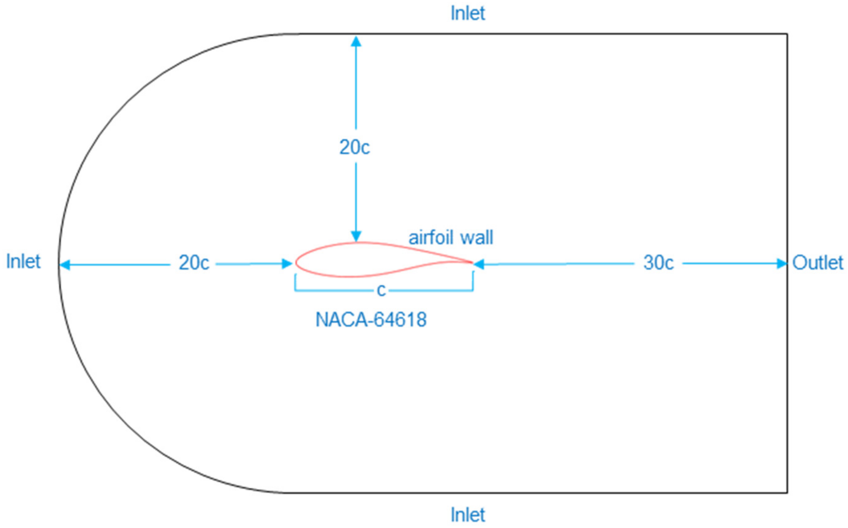
The DesignModeler software, available in ANSYS, was used to build the geometric model. As illustrated in
Figure 1, we considered a large computational domain to capture all essential flow disturbances, especially downstream. The boundary positions and the domain size are based on previous works, which showed good agreement with experimental and numerical data [
20,
44,
45]. Such distance is large enough to make sure that the boundary conditions assigned to the outer domain do not alter the flow next to it and affect the quality of results. The adequacy of the dimensions of domain control has been demonstrated through the resulting velocity streamlines and the pressure contours around the airfoil illustrated in the results section (Figure 13).
Once the geometric models were created, the mesh was generated. As illustrated in
Figure 2, the adopted mesh (no. 4 in
Table 3) has as its main characteristics tetrahedral elements throughout the domain and layers of prismatic elements close to the solid wall of the airfoil, allowing us to consider the boundary layer phenomena. In addition, a mesh with a dimensionless distance
y+ ≤ 1 was generated to address the viscous sublayer.
2.2. Mesh Independency Study
Five meshes were generated to perform a mesh convergence verification by modifying the number of elements. Local refinement of the mesh was chosen, i.e., the differences in the spatial discretization are localized around the airfoil. We started with a coarse discretization on the upper limit of the boundary layer and refined discretization on the profile wall (see
Table 3).
In all the meshes, the prismatic layer was composed of 30 layers (according to the literature consulted) whose initial height was 4.5 × 10
−6 m, derived by taking
y+ less than 1. The estimation of initial height was calculated using Equation (1) [
46].
where
is the initial height (wall distance),
is the dimensionless wall thickness parameter,
is the dynamic viscosity of air,
is the air density, and
is the friction velocity calculated using Equation (2):
where
is the wall shear stress, calculated using Equation (3):
where
is the skin friction calculated using the Schlichting skin-friction correlation represented in Equation (4):
The initial height was computed using the parameters in
Table 4. It is important to mention that the air properties have been considered for a temperature of −10 °C.
The CFD independency study involved calculations with different meshes to evaluate the convergence of the most relevant variables. In our case, the lift and drag coefficients were chosen. The validation results of the above five meshes are presented in
Table 5. The convergence error was calculated as a percentage of the difference between the coefficient results of two successive meshes.
As seen in
Table 5, the last two meshes have comparable errors; hence we can use either mesh 4 or 5. However, considering the computational cost (time required for the simulation), mesh no. 4 was chosen to continue the simulations. In addition, as can be seen in
Figure 3, the behavior of the lift and drag coefficients reached a constant value for the last three meshes, demonstrating that the solution is not mesh-dependent.
3. Results and Discussion
The presented results show the validation of the resulting NACA 64-618 aerodynamic parameters with experimental data and comparison with the results of a numerical study found in the literature for this airfoil [
10,
25]. In addition, the turbulence issue is addressed through CFD simulations in combination with two scenarios of roughness consideration.
Turbulence is described in the literature as a stochastic process. Flow is turbulent in practically all wind turbine applications, especially when ice is present. Because of the complexity of turbulent flows, no analytical solution can effectively predict airflow changes in turbulent zones. Turbulence modeling should consequently be consistent with the numerical solution of nonlinear partial differential equations of flow. It may be represented in terms of time-averaged equations of motion for fluid flow using statistical methods such as the Reynolds average statistical approach rather than merely the physical method. The CFD solution for turbulence modeling usually depends on the Reynolds-averaged Navier–Stokes (RANS) equations [
30].
Several models are often employed in CFD simulations to account for turbulence development in aerodynamic calculations, notably the Spalart–Allmaras,
k-ε,
k-ω, and
k-ω SST, which have been extensively utilized in flow modeling around icing-contaminated airfoils in wind turbines. These models correspond to the Reynolds-averaged Navier–Stokes (RANS) family [
47], which has been widely studied in the literature for wind turbines [
48,
49]. The
k-ε turbulence model is based on turbulent kinetic energy and dissipation rate. As a result, it is also known as the two-equation turbulence model. This model performs well for totally turbulent flows. It is used to compromise acceptable computing costs and needed accuracy in turbulent flow simulation [
35]. The
k-ω SST shear stress transport turbulence model combines the advantages of two models in different flow regions. The standard
k-ω model is activated near the airfoil’s walls, and the
k-ε model is away from the wall. The
k-ω SST benefits the modeling flows around wind turbine blades thanks to analyzing the boundary layer laminar-turbulent transition at high angles of attack [
36]. The Spalart–Allmaras model is a one-equation model. Initially created for aerospace, this turbulence model is frequently utilized in wind turbines due mainly to its acceptable computing cost and precision in modeling turbulent flow [
25,
50]. However, since this model has a disadvantage in the transition zone at high angles of attack compared to the
k-
w model, in this study we wanted to examine its performance with moderate ice accretion conditions, which increase turbulence at the suction side of the airfoil.
3.1. Clean Airfoil
To estimate the aerodynamic loss due to icing, we first had to estimate the aerodynamic parameters for the clean airfoil. Then, to validate the simulation, we compared the results with experimental data from [
10] for the same clean airfoil. The validation consists of verifying the clean airfoil’s aerodynamic behavior under different angles of attack. We also compared the results with the study by Homola et al. [
25] using the same turbulence model (Spalart–Allmaras).
As shown in
Figure 4, the lift coefficient agrees with the experimental data and is slightly lower than those presented by [
25]. This could be explained by the differences in the tools and the setup used for the simulation, such as mesh type, elements, number of nodes, and other mesh characteristics. Regarding the drag coefficient (
Figure 5), the results were in good agreement with both cases but slightly higher, with the exception of an angle of attack of 15°. In this case, the experimental result was significantly higher than the estimation obtained with CFD. This could be associated with a discrepancy in the measurement process due to the stall phenomenon. However, Etemaddar and Hansen [
10] mentioned that the uncertainty in experimental drag coefficient measurement is higher than for the lift coefficient. Therefore, the agreement with the experiments is not perfect but considered acceptable.
In the same way, it is also known that the Spalart–Allmaras turbulence model has drawbacks in areas of high-pressure gradients [
32]. However, the discrepancy between the experimental data and the numerical drag results for the clean airfoil at high angles of attack was considered less critical since it occurs outside the operating ranges of the referenced wind turbine [
25].
Given that icing increases the chance of flow separation, in the remainder of this paper we wanted to investigate the performance of the Spalart–Allmaras model in the presence of ice by comparing its results with those obtained using the k-ω SST turbulence model.
3.2. Iced Airfoil
The iced airfoil validation verified the ice shape obtained under the same icing conditions as in [
25]. Then, the validation of the lift and drag coefficients was performed.
As shown in
Figure 6, the ice accumulated at the leading edge was as expected. A small fraction of the collected supercooled water does not freeze immediately upon impact with the leading edge of the airfoil, causing the water to run back to freeze later at the trailing edge outside the impingement area as observed in [
51].
Figure 7 shows a small accumulation of ice occurred at the trailing edge, modifying the pointed shape of the airfoil.
Regarding the leading edge (see
Figure 8), the ice shape was similar to the one presented in [
25] with more details on the outer surface, which allows us to state that the model and the adopted simulation tools have good replicability. However, in this case it was impossible to validate with an experimental study due to insufficient information on how the experiment was conducted (temperature, velocity, LWC, MVD, etc.).
3.3. Effect of Surface Roughness Distribution
Roughness is a crucial factor for icing modeling accuracy. Multiple authors have mentioned the importance of roughness in icing simulation [
5,
39,
44]. Airfoil performance is very sensitive to roughness since it affects boundary layer transition, leading to flow separation [
44,
52]. In the presence of ice, even in small quantities, the airfoil’s aerodynamic performance is degraded. It is therefore important to account for roughness effects at every step of ice growth calculation [
52]. The roughness height is an essential parameter to consider when modeling wind turbine icing because it affects the calculation of the convective heat transfer coefficient, which is fundamental in heat transfer analysis [
53,
54]. Aircraft icing modelers employed CFD extensively to examine the local heat transfer coefficient across aircraft components, indicating that surface roughness may significantly enhance local heat transmission even with a thin coating of ice [
55].
Each research center usually describes roughness differently. For example, the conventional NACA roughness model is created by employing typical grain sizes dispersed equally from the leading edge downstream on the pressure and suction surfaces (typically to 7.5% of the chord length) [
56]. The Shin et al. [
38] sand-grain roughness model, developed initially for aeronautics, is one of the most-often used correlations for estimating ice surface roughness over wind turbine blades. The empirical correlation is based on the Shin and Bond formula, which calculates the height of small-scale surface roughness:
k/c (mm) as a function of static temperature
T (°C), airfoil chord length
c (m), median volume diameter (µm), liquid water content (g/m
3), and the relative wind speed
V (m/s). The beading model available in ANSYS-FENSAP-ICE performs implicit estimations of surface sand-grain roughness distribution. The computation of constant and variable sand-grain roughness distributions is incorporated into the three available turbulence models [
39]. When the beading model in ANSYS FENSAP-ICE is selected, the sand-grain roughness output is automatically activated [
39]. The Shin and Berkowitz [
38] sand-grain roughness is used as described in Equation (5) from FENSAP-ICE documentation [
39]. Almost all wind turbine icing CFD studies depend on this model for roughness calculations [
5,
57]. The empirical correlation estimates the small-scale surface roughness height
ks/
c (mm) as a function of airfoil chord length (m), the relative wind speed (m/s), the liquid water content (g/m
3), the median volume diameter (µm) and the air temperature (°K).
To examine the effect of considering roughness throughout the phases of growing ice simulation, we conducted a multi-shot simulation of ice growth around an NACA 64-618 airfoil using the beading model. We conducted simulations on a clean and iced NACA 64-618 for angles of attack of 0, 5, 10, and 15 degrees using the Spalart–Allmaras and
k-ω SST turbulence models separately.
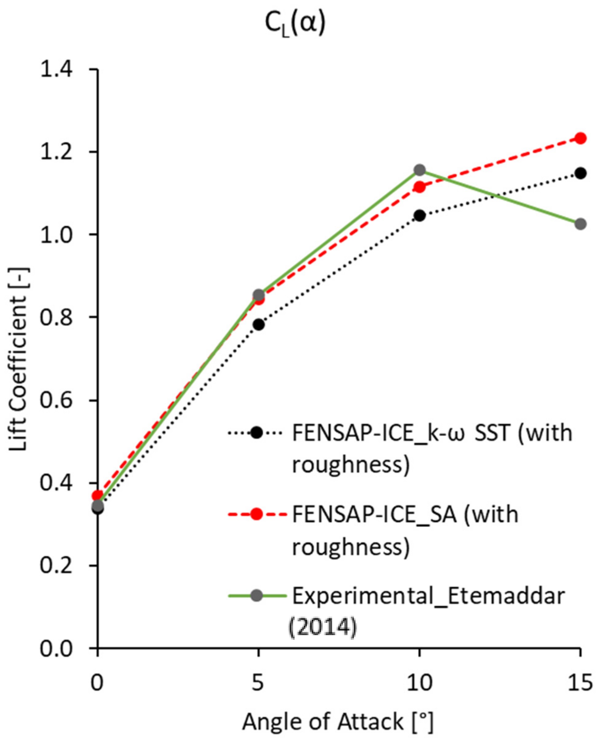
Figure 9 and
Figure 10 show the results for the lift and drag coefficients, respectively. We compare [
25] (plain line) with the lift and drag coefficients with no roughness (dashed black line), and with the Shin et al. [
58] roughness model available in FENSAP-ICE (dotted red line).
When the roughness was not considered in the simulation, the resulting lift coefficient was higher than its value with a no-ice airfoil, while the drag coefficient was lower. The results obtained when not considering the roughness led to results that were contrary to what is known in the literature. When roughness was considered, the results were convincing and closer to those obtained by [
25], with some differences at higher angles of attack. The average difference was about 9.42% for the lift coefficient and 19.51% for the drag coefficient for iced airfoils.
To evaluate the effect of considering roughness on the aerodynamic performance loss estimation, we calculated the percentage of aerodynamic losses of the iced airfoil compared to the clean airfoil for each case. As seen in
Table 6, when roughness was not included in the calculations, the average loss in lift coefficient was estimated at 7.50% using Spalart–Allmaras and at 1.96% using
k-ω SST. When considering roughness in the simulation (see
Table 7), the average loss in lift coefficient due to icing was estimated at −15.94% using Spalart–Allmaras and −22.54% using
k-ω SST. For the drag coefficient, the average gain for the iced airfoils (increase in drag) using Spalart–Allmaras was 9.30% for the case without roughness consideration and 140.93% with roughness consideration. For the
k-ω SST model, the increase in drag was 30.91% without roughness and 178.78% with roughness. Therefore, not considering roughness in the calculations seriously affects the simulation results and underestimates the effect of ice on aerodynamic performance.
3.4. Effect of Turbulence Model
The choice of turbulence model also influences the simulation results. Based on the conclusion of the previous subsection, the comparisons between the two turbulence models were made considering the roughness effect in the simulation. As seen in
Figure 11, the lift coefficient was lower with
k-ω SST. A 14.86% difference compared to Homola et al. [
25] is estimated. When comparing the results using
k-ω SST with those using the Spalart–Allmaras model, the difference was approximately 7.19%. Similar behavior was observed for the drag coefficient (see
Figure 12). In this case, the difference compared to Homola et al. [
25] was about 20.21%, while the difference between the two turbulence models was 3.13%. Except for the high angles of attack, the differences between the two turbulence models were minor, indicating that the influence of the choice of turbulence model on the resulting aerodynamic losses due to icing is limited compared with that related to roughness consideration. Once again, the discrepancy between the experimental data and the numerical results for the iced airfoil at high angles of attack was considered less critical since it occurs outside the operating ranges of the referenced wind turbine [
25].
To further investigate the turbulence model effect on the iced airfoil simulation, we used the two turbulence models to compare the behavior of the pressure and velocity fields as well as streamlines for clean and iced airfoils.
Figure 13 shows the flow patterns for the angle of attack of 5.824°, which is for the airfoil located at 95% spanwise (relative to the radial distance of the section position on the wind turbine blade). It demonstrates the velocity streamlines with pressure contours resulting from the use of each turbulence model:
k-ω SST (right) against Spalart–Allmaras (left). Concerning the pressure contours, with the
k-ω SST model, the pressure was lower at the suction side of the airfoil. The maximum pressure at the leading edge was also lower than that calculated with the Spalart–Allmaras turbulence model. Regarding the streamlines in the iced airfoil, both turbulence models presented a recirculation zone at the trailing and the leading edge (red circles). However, the
k-ω SST model showed better results in the leading-edge recirculation area than the Spalart–Allmaras (see
Figure 13e,f). The streamlines around the recirculation zone in
Figure 13f have been better detailed to demonstrate the model’s efficacy in simulating the turbulence zones.
3.5. Analysis of the Aerodynamic Performance of the Iced Airfoil
Figure 14 and
Figure 15 show comparisons between the aerodynamic coefficients for both clean and iced airfoils. As expected, with the presence of ice, the lift coefficient decreased (
Figure 14) while the drag coefficient increased (
Figure 15). This is in agreement with the results in the literature.
The predicted lift loss was more significant with the k-ω SST model, with an average difference of 7.19%. At the same time, the increase in drag was similar for both turbulence models, with an average difference of 3.13% between the two models. For the clean airfoil, the two turbulence models give similar results, with a slight difference in the drag prediction at an angle of attack of 15 degrees. This is due to the proximity to flow separation conditions at the suction side of the airfoil. As discussed, the Spalart–Allmaras turbulence model has drawbacks under boundary layer separation conditions, which manifest more in the presence of ice on the airfoil.


 ,
, 


