Mean Flow, Turbulent Structures, and SPOD Analysis of Thermal Mixing in a T-Junction with Variation of the Inlet Flow Profile

Abstract

This paper investigates the effects of different inlet flow profiles on thermal mixing within a T-junction using CFD simulations with the IDDES-SST turbulence model. The different combinations of inlet flow profiles are related to different stage in the flow entry region. The effects of the inlet flow profile on the mean and transient flow behaviour are assessed, while a spectral proper orthogonal decomposition and power spectral density analysis are performed to assess the underlying flow structures and the predominant frequency modes. It is found that the vortical structures associated with the horseshoe and hovering vortex systems consist of a single roll-up vortex for cases with uniformly distributed boundary conditions (BCs) at the branch inlet whereas a double roll-up vortex is observed for the other cases. The double roll-up vortex enhances the mixing locally due to the entrainment of fluid from the branch pipe in these vortical structures, which then results in a lower mean temperature distribution. The appearance of the secondary vortex pair and the nested vortices is delayed for cases with uniformly distributed BCs at the branch inlet, which again results in lower thermal mixing and consequently higher values of mean temperature when compared with the other cases. It is also found that the vorticity related to the counter-rotating vortex pair as well as to the second pair of vortices rotating in the opposite direction is higher for cases with uniformly distributed BCs at the branch inlet. Lastly, the combinations of inlet flow profiles lead to different coherent structures, and the dominant frequencies are of a Strouhal number of around 0.7 for uniformly distributed profiles at the branch inlet and in the range 0.4–0.5 for the other cases.

1. Introduction

The mixing of fluid streams with different temperature in system pipelines is of interest to many areas of engineering. In nuclear power plants (NPPs), T-junctions are one of the common components where fluids at different temperatures mix and can be found within primary and secondary nuclear thermal-hydraulic circuits, as well as safety lines [1]. The interaction between the two fluids is often highly turbulent and can result in an incomplete mixing and, on a larger scale, can lead to damage to the pipe structure induced by thermal fatigue [2,3,4]. The key factors that can cause thermal fatigue near the T-junction are (1) thermal cycling, which is the process of cycling of the interface of thermally stratified fluids [5], and (2) thermal striping, which is defined as a quasi-random temperature fluctuation produced by the incomplete mixing of fluids [6,7]. Several pipe failures and leakage incidents in NPPs have been attributed to thermal striping and fatigue [8,9,10], which highlights the need to better understand the flow physics underlying thermal fatigue for plant safety and long-term component reliability, as well as plant aging assessment and life extension (PLEX) [11,12].

T-junction flows have been the subject of studies in recent decades and represent considerable challenges due to the complexity of the phenomena involved. Flow visualization techniques, used to investigate different velocity ratios and Re numbers, reveal the presence of coherent vortical structures in the region between the incoming jet from the branch pipe and the crossflow from the main pipe with periodical shedding character, interlocking vortices and ring-like vortices produced by the shear-layer roll-up [13]. In this study, it is also shown the presence of a set of unsteady horseshoe vortices upstream of the T-junction on the left-hand side of a stagnation point, whose vortex lines bend around the jet. Flow visualisation techniques in jet-in-crossflow reveal coherent vortical structures similar to what it is found in T-junction flows [14,15,16,17], indicating a similarity between these types of flows. Horseshoe vortices originating just upstream of the jet are also observed in visualisation studies of jet-in-crossflow for different velocity ratios [18,19].

Flow reversal and recirculation phenomena are observed in T-junction flow studies downstream the jet entrance into the main pipe [13,20], together with the presence of bubble-type vortex breakdown phenomena [21]. The phenomenon of vortex breakdown, and associated flow reversal, are also observed in ref. [18] and found to be connected to the mixing properties of a jet-in-crossflow. In ref. [20], it is shown that the regions of concentrated vorticity are distributed in three pairs of counter rotating vortices, which is also observed in jet crossflow [22]. The primary counter-rotating vortex pair, CVP, known also as a ‘bound vortex’ in the jet-in-crossflow literature, forms the dominant structure further downstream of the T-junction. Visualizations of the wake of the jet in T-junction flows, and the jet-in-crossflow, reveal a resemblance to three-dimensional Karman vortex streets, where the jet acts similar to a solid body with respect to the main flow [13,18,19].

Computational fluid dynamics (CFD) methods have also been used to provide insights on T-junction flows. Detailed validations of the CFD methods are required to produce accurate models and simulations (M&S) of the complex phenomena in T-junction flows. Significant effort was devoted to generating validation benchmark datasets to improve the capability of the CFD methods to reproduce the complex phenomena in T-junction flow. The OECD/NEA-Vattenfall T-junction Benchmark is an example of validation benchmark test case conducted with water at mild temperature and adiabatic wall conditions [23,24]. The MOTHER project is a more recent example of validation benchmark test case conducted with water at similar temperature conditions which includes heat transfer and temperature measurements within the T-junction pipe wall [25,26].

The validation benchmark datasets provided by these benchmarks have been used to assess different CFD M&S approaches for mixing T-junction flows. In ref. [27], it was shown that simple Reynolds-Average Navier-Stokes (RANS) turbulence models fail to accurately capture the turbulent nature of these flows with poor agreement found in the predictions of temperature and velocity fluctuations. In contrast, predictions obtained from more sophisticated turbulence models, such as Large Eddy Simulations (LES), show good agreement with the experimental data [27,28,29]. In ref. [28,29], however, it was also shown that the use of a non-sufficient near-wall resolution in LES can result in poor temperature fluctuation predictions close to the wall. Results from wall-resolved LES simulations show better agreement close to the wall but at a higher computational cost due to the much finer mesh requirements [30]. Performances from alternative near-wall methods, such as a hybrid RANS-LES Detached Eddy Simulation (DES) were also investigated and compared with LES performances [27,28]. In these studies, DES predictions showed promising results, but still not as good as LES. Studies which use newer developments of the DES model, i.e., the Delayed DES (DDES) and the Improved DDES (IDDES), showed higher performances compared with the DES model [31,32,33,34,35]. Indeed, in ref. [33,34,35], predictions of the IDDES model agreed quite well with the experimental data, showing the ability of this model to accurately simulate thermal mixing in T-junctions.

Inlet flow profiles of the boundary conditions (BCs) need also to be correctly prescribed to avoid errors and inaccurate CFD predictions [36]. However, few studies present a comprehensive analysis for T-junction flows regarding the inlet flow profiles of the BCs. A common assumption is to use uniformly distributed or fully developed inlet flow profiles for the CFD simulations. These simple assumptions may lead to different mean and transient flow behaviours and hence result in different mean temperature distributions and temperature fluctuations at the pipe wall. These temperature fluctuations may lead to temperature oscillations with frequencies in the range of high cycle thermal fatigue as shown in our previous studies [33,34,35,37,38].

The aim of this paper is to systematically assess the effects of different combinations of inlet flow profiles on the mean flow and turbulent flow structures using CFD simulations with the IDDES-Shear Stress Transport (SST) model. A brief description of the computational model is presented in Section 2 and the general flow structure is given in Section 3. Finally, Section 4 presents the effects of different inlet flow profiles on the mean flow, vortex structure, turbulent quantities, and transient flow.

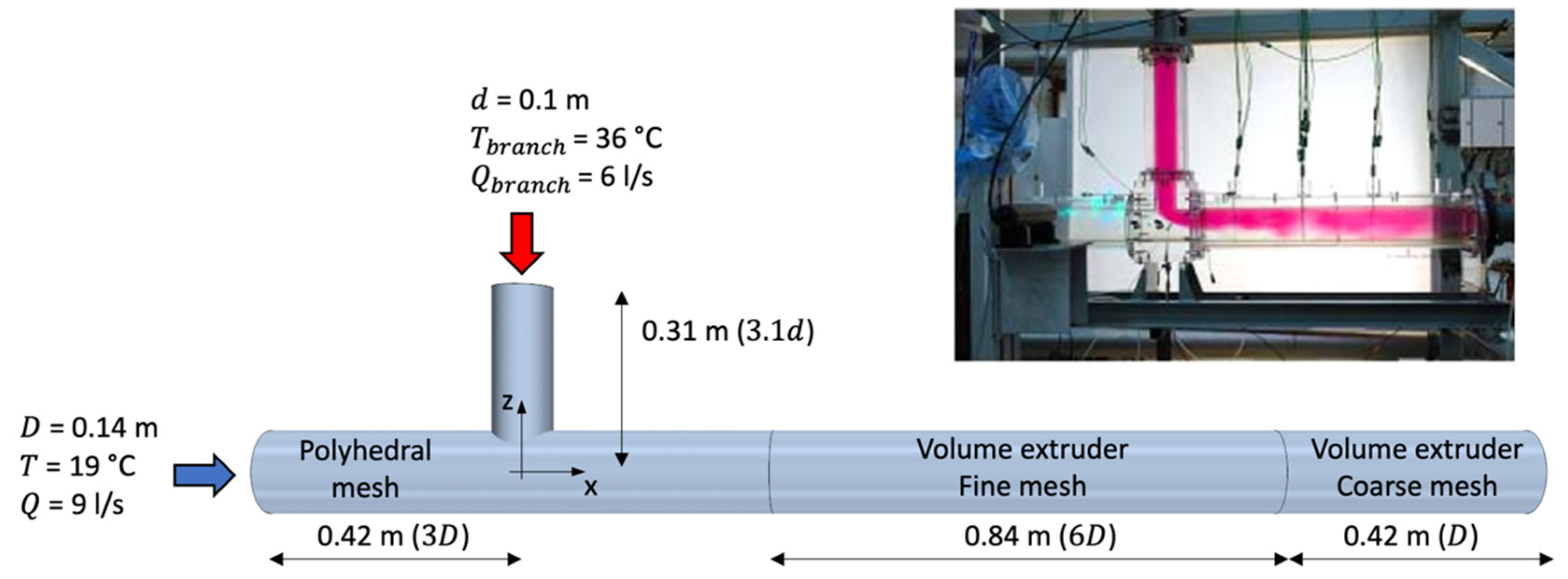
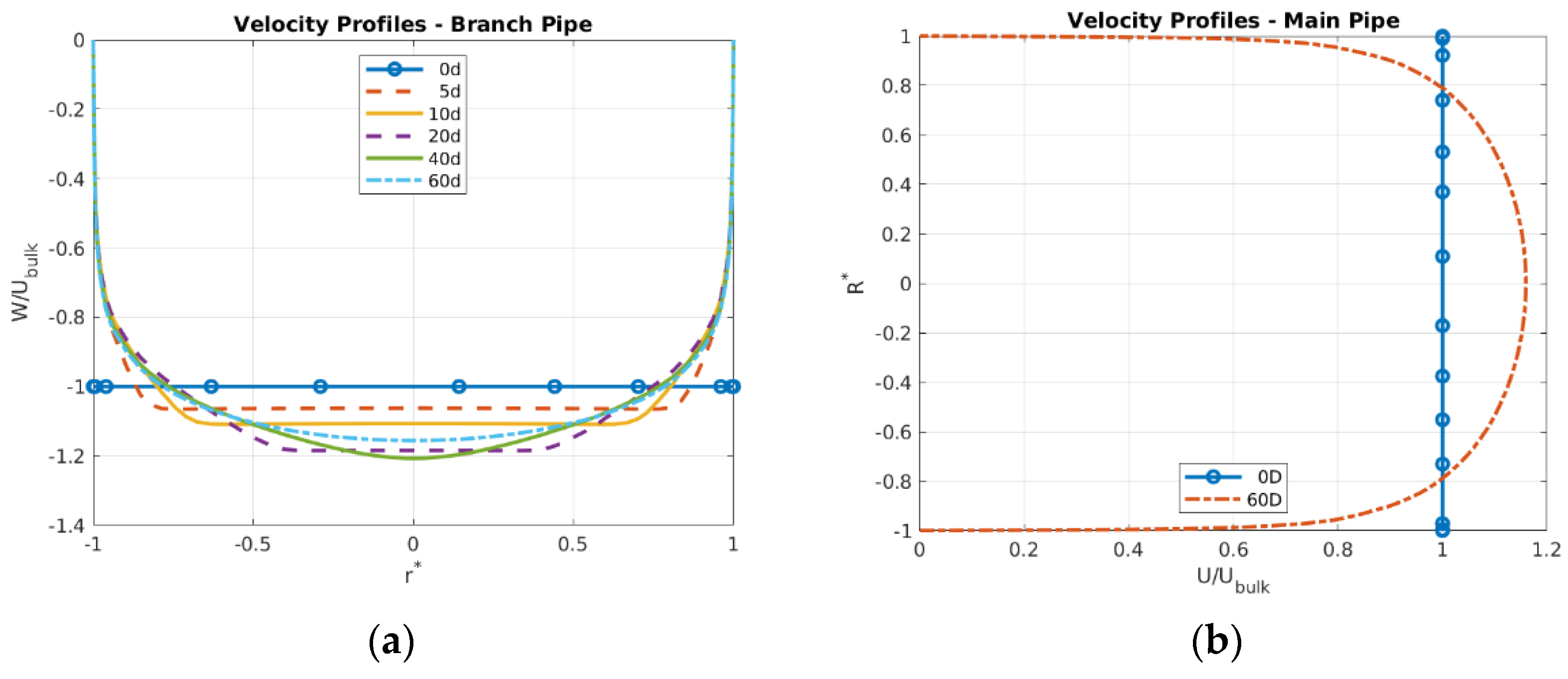
2. Description of the CFD Models

The T-junction test case, of reference for this study, is the experimental test rig used in the OECD/NEA-Vattenfall T-junction benchmark [23,24]. In our CFD model, the flow domain comprises two major components, the T-junction and outlet pipe. The T-junction, formed by the main pipe with diameter $D$ and branch pipe with diameter $d$, extends for 6$D$ in the x-direction, and 3.1$d$ in the z-direction, whereas the outlet pipe extends for a total length of 9$D$ (see Figure 1). For the sake of clarity, the CFD models will be named as the “T-junction model” in our following discussion.

A polyhedral and prism layer computational mesh is used in the T-junction section while other regions are meshed using the volume extruder available in the commercial CFD code Simcenter STAR-CCM+ version 2020.1.1 [39]. The turbulent flow is modelled using the IDDES-SST [40] turbulence model. The IDDES-SST is a hybrid RANS/LES model which uses RANS close to the wall and LES in the bulk flow. The RANS and LES regions across the computational model are shown in [33] for different mesh sizes and in [37] for different BCs.

A higher order discretization scheme, the MUSCL 3rd order central difference spatial discretization scheme, is used as suggested in [31]. The time step size is $5\times {10}^{-4}$ s, which yields to a CFL number that is in general, lower than 0.5. Three different set of meshes are assessed with a total number of cells of 2.08 million, 3.42 million, and 7.42 million which result in values of $y^{+}$ generally lower than 1 in all meshes and a maximum grid step for the finest mesh in the streamwise direction of ${\Delta }_x^{+} \approx$ 80. The results of the mesh sensitivity study and model validation are reported in [33]. To reduce the numerical error, the most refined computational mesh is used for the rest of the discussion.

The inlet flow profiles of the T-junction models are generated with separate CFD models, i.e., inlet flow profile generators for the main pipe and branch pipe. The flow in the inlet flow profile generators is modelled using RANS k-ω-SST [41] turbulence models. The bulk velocity for the inlet flow profile generator of the main pipe is 0.585 m/s, and it is 0.764 m/s for the inlet flow profile generator of the branch pipe. The inlet values for the turbulent kinetic energy and specific dissipation rate are assumed to be constant with values of 0.001 J/kg and $1\times {10}^{-4}$ s⁻¹, respectively. The inlet temperatures are 19 °C for the main pipe and 36 °C for the branch pipe. The computational domains of the inlet flow generator are meshed using the volume extruder from the T-junction inlet sections. The length of the pipes of the inlet flow profile generators is set as 80 diameters to assure that fully developed flow conditions can be achieved at the T-junction inlets. Fully developed flow is reached at around 60 diameters from the inlet section of the main and branch pipes.

The inlet flow profiles of velocity, turbulent kinetic energy, and specific dissipation rate obtained at different developing stages are then supplied as BCs to the inlets of the T-junction computational model. Uniformly distributed flow profiles are also considered. These uniformly distributed velocity profiles are set to the bulk velocities of the respective inlets. Fully developed conditions refer instead to the profiles extracted at 60 diameters downstream the inlets of the inlet flow profile generators. In ref. [33], it is shown that the inlet flow profiles of the BCs at the branch inlet have the most significant impact on the thermal mixing downstream of the T-junction. To further understand the flow physics behind this observation, uniformly distributed BCs, indicated with the index ‘0’, and profiles extracted at 5, 10, 20, 40, and 60 diameters from the inlet flow profile generator of the branch inlet pipe are considered as the inlet of the branch pipe of the T-junction (branch inlet for short). Only uniformly distributed BCs and fully developed profiles are considered at the inlet of the main pipe of the T-junction inlet (main inlet for short). The velocity profiles used for the main and branch T-junction inlets are shown in Figure 2 with respect to the non-dimensional radius $R^{*}=2r/D$ for the main pipe, and $r^{*}=2r/d$ for the branch pipe, where $r$ is the radial coordinate. The combinations of BCs for the sets of inlet flow profiles investigated in this study (12 in total) are summarised in

Table 1. Summary of inlet flow profiles of the BCs. Each simulation is identified with a pair of indices; the first index represents the inlet flow profiles used at the main T-junction inlet, and the second index refers to the inlet flow profiles applied to the branch T-junction inlet.

Case	Main Inlet BC	Branch Inlet BC	Case	Main Inlet BC	Branch Inlet BC
‘0-0’	0D	0d	‘60-0’	60D	0d
‘0-5’	0D	5d	‘60-5’	60D	5d
‘0-10’	0D	10d	‘60-10’	60D	10d
‘0-20’	0D	20d	‘60-20’	60D	20d
‘0-40’	0D	40d	‘60-40’	60D	40d
‘0-60’	0D	60d	‘60-60’	60D	60d

. Each simulation is identified with a pair of indices; the first index represents the inlet flow profiles used at the main T-junction inlet, and the second index refers to the inlet flow profiles applied to the branch T-junction inlet.

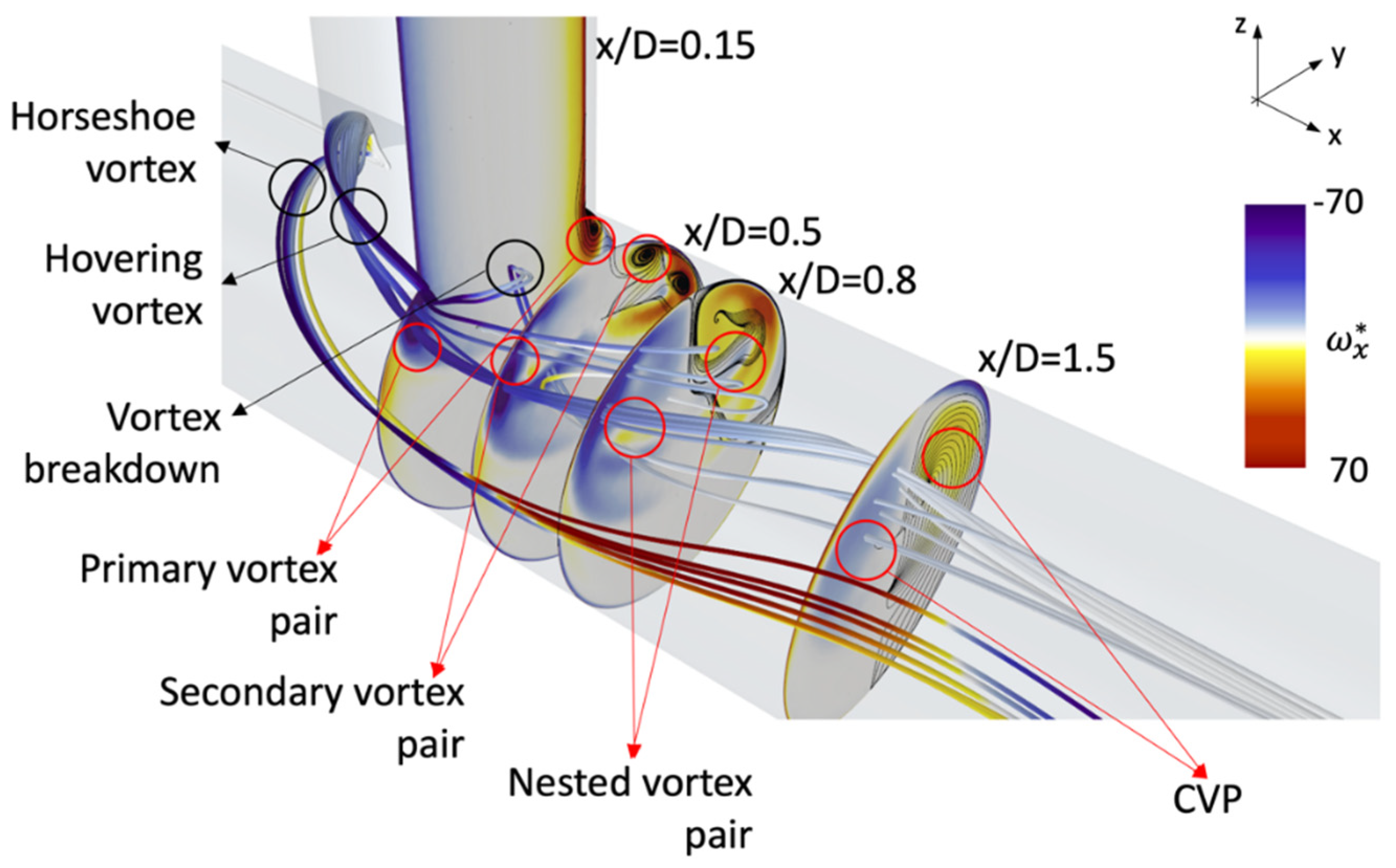
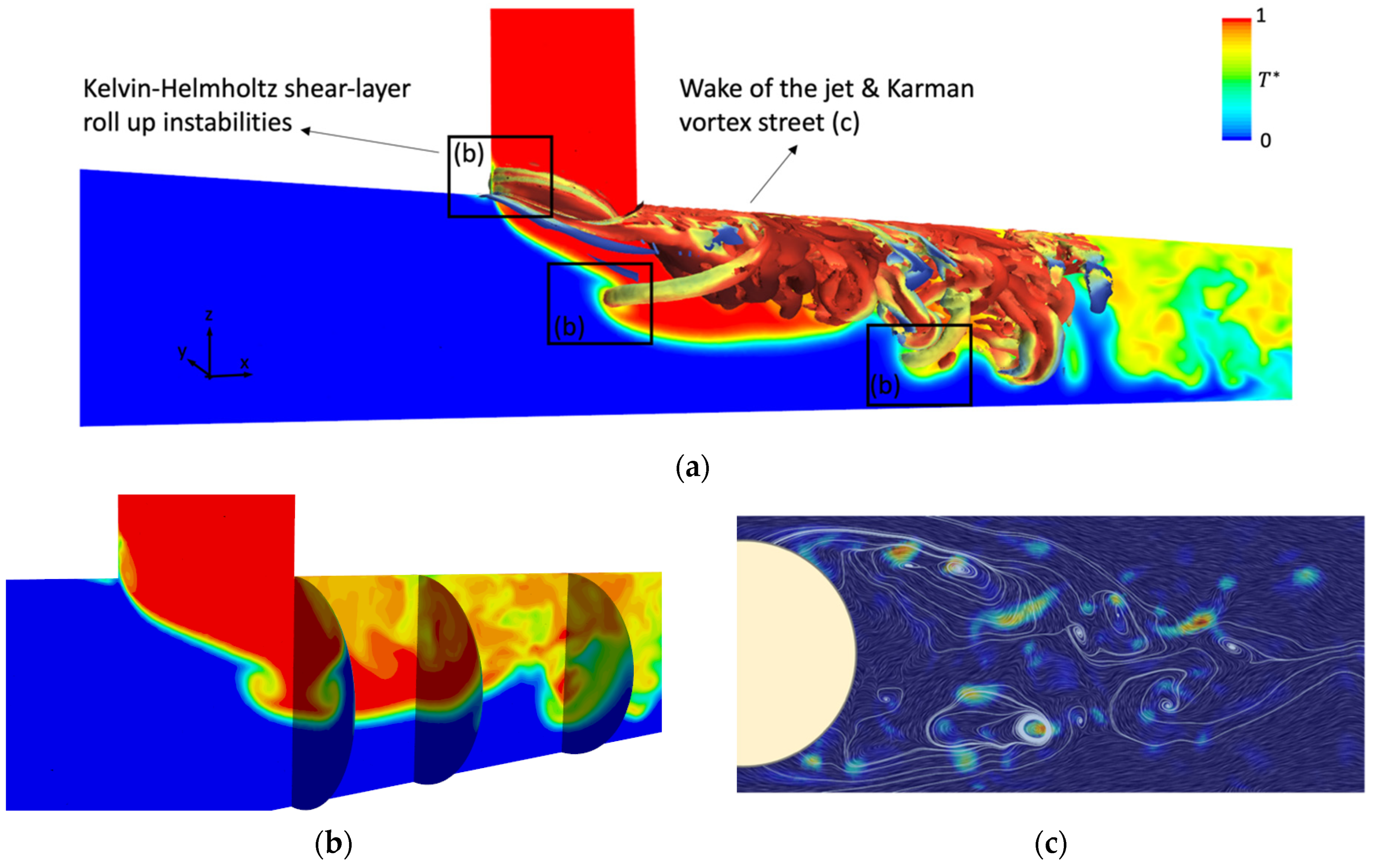
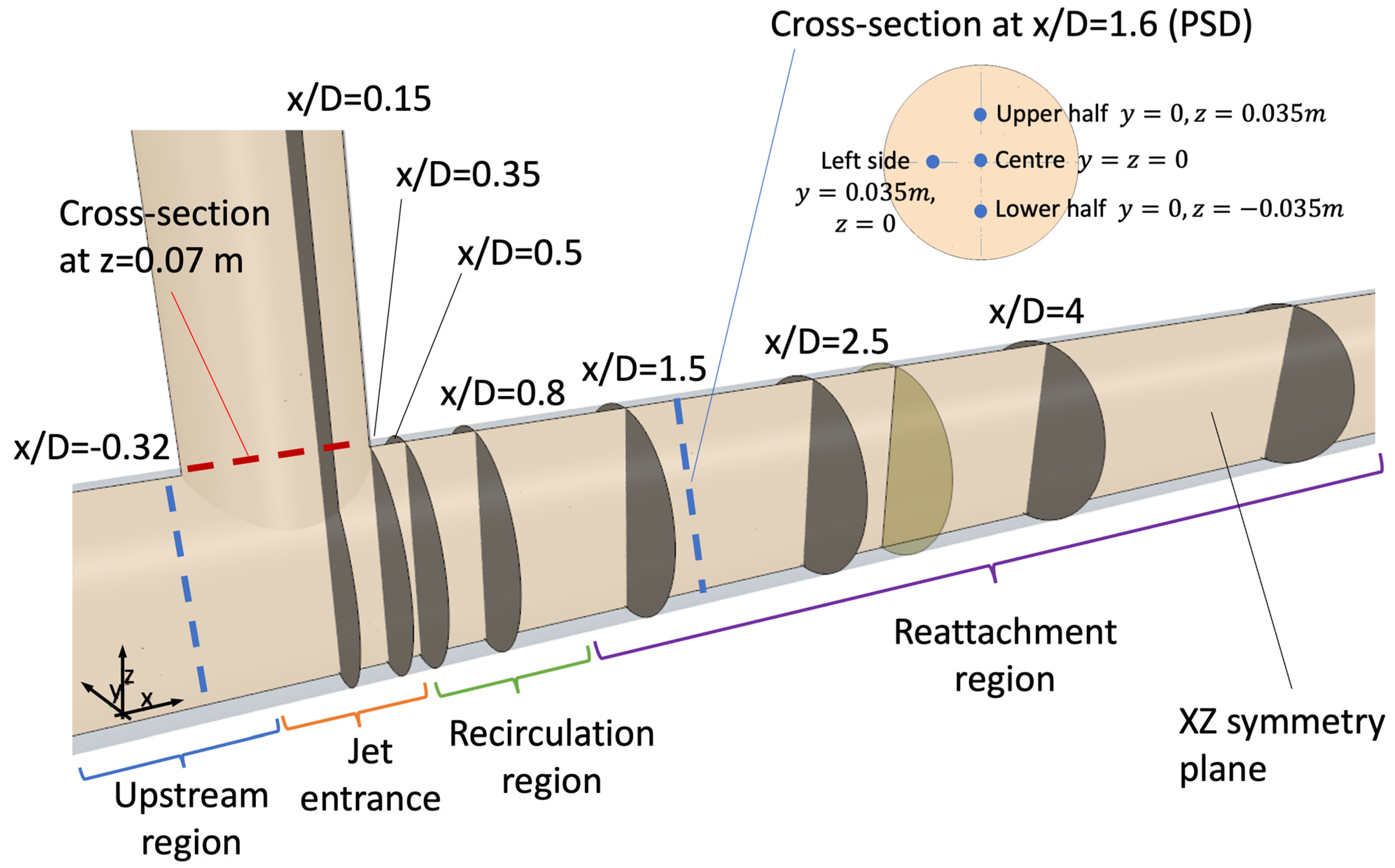
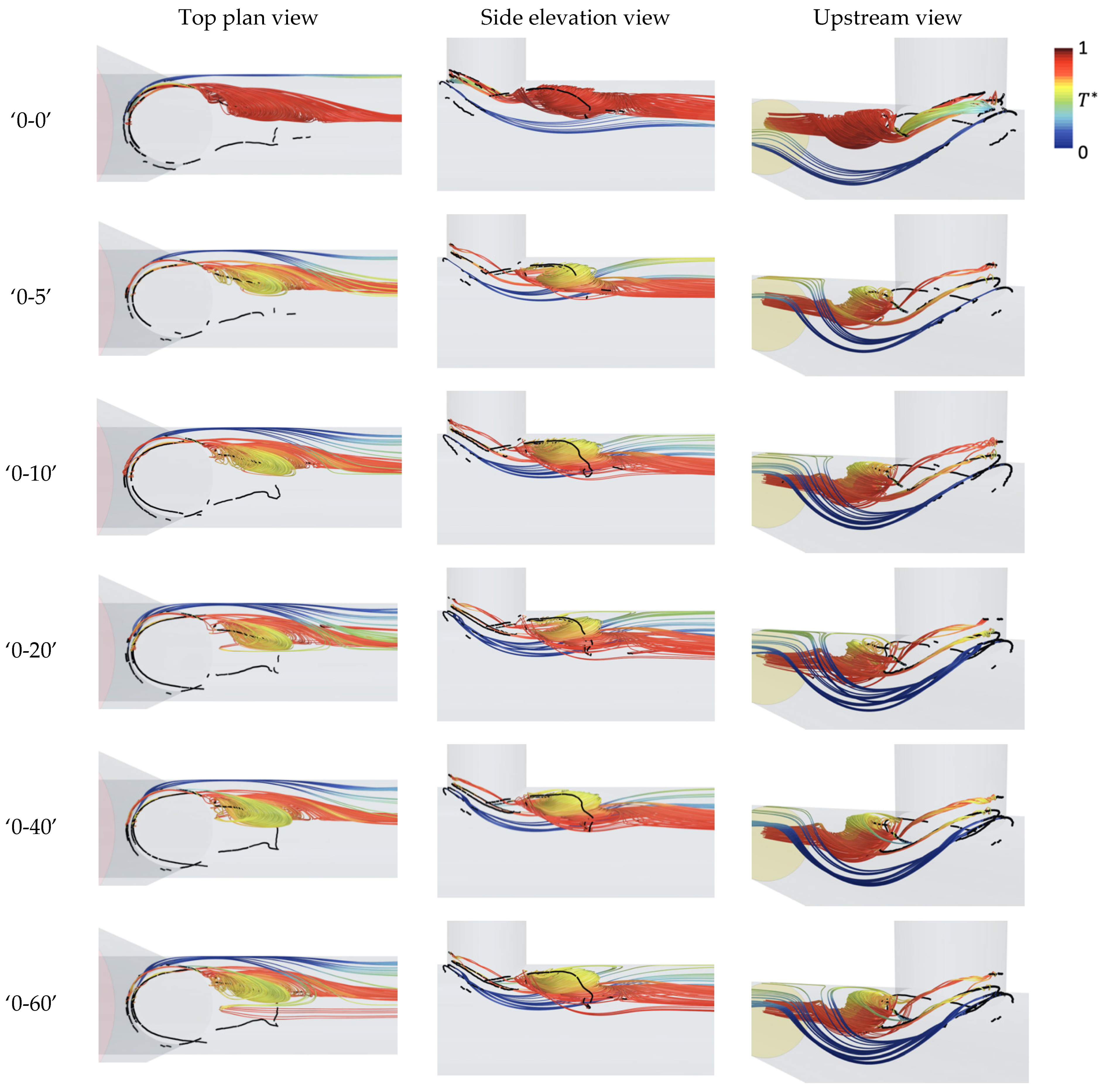
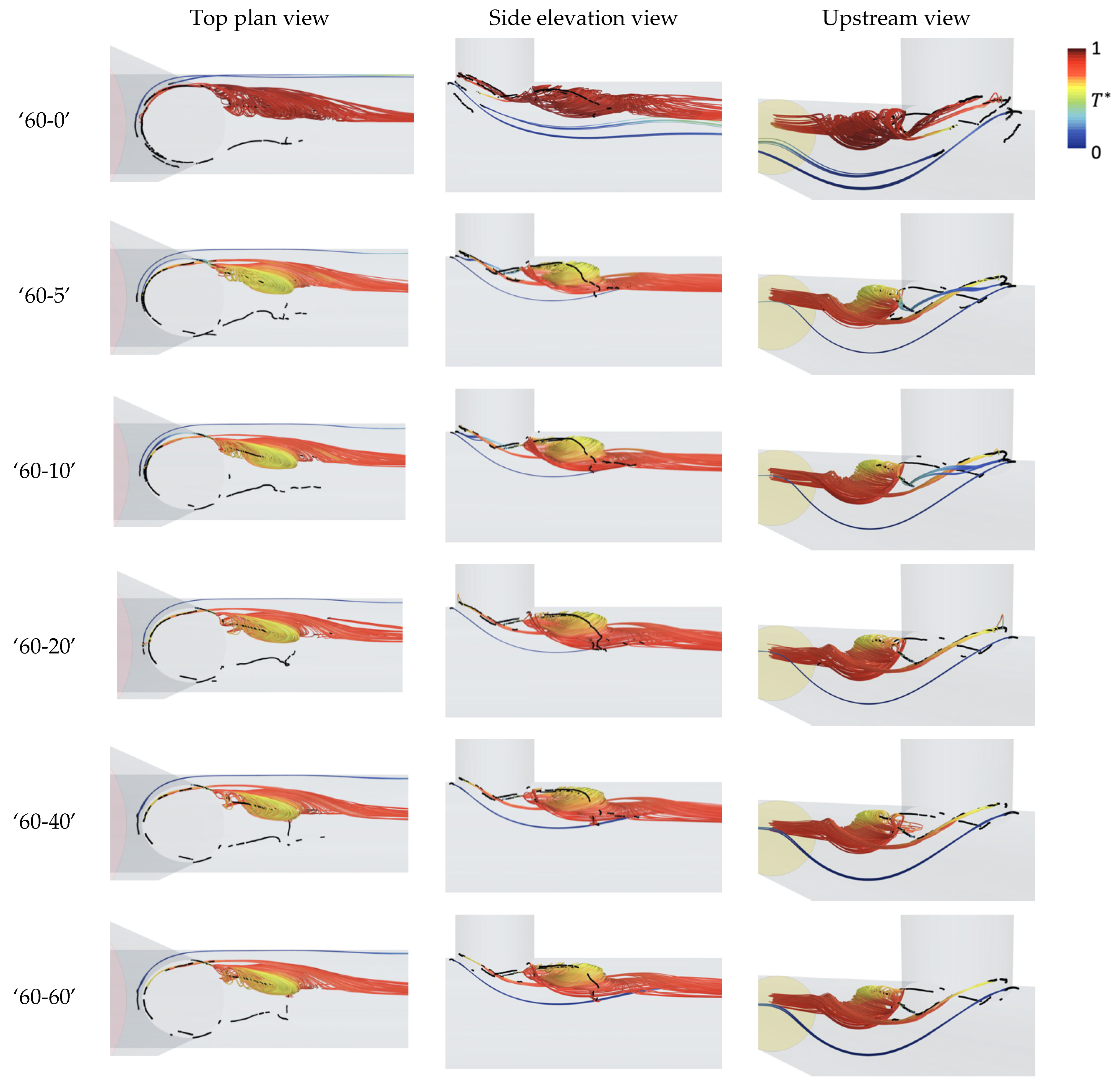
3. Overview of the Flow Structure

The jet flow pattern is characterised by the value of the momentum ratio [42,43], $M_R$, which represents the ratio between the momentum of the main pipe, $m$, and the momentum of the branch pipe, $b$, defined as:

$$M_R=\frac{D_m{D}_b{\rho }_m{V}_m^2}{\pi {\left(\frac{D_b}{2}\right)}^2{\rho }_b{V}_b^2}.$$

(1)

The values of $M_R$ and of the velocity ratio of the test facility used in the OECD/NEA-Vattenfall Benchmark are 1.05 and 1.3, respectively. According to [42,43], the jet from the branch pipe, in this study, can be classified as a deflecting jet. The jet from the branch pipe detaches at the downstream edge and flows mainly in the central part of the main pipe, bending in the direction of the main flow. To assess the mean flow and turbulent structures, the computational domain is divided into four regions as shown in Figure 3: the upstream region, the jet entrance region, the recirculation region, and the reattachment region.

The mean flow structures for each region are presented in Figure 3 using the streamlines and vectors contours of the mean velocity field. In the upstream region, as the jet enters the main pipe, it produces an adverse pressure in the vicinity of the upstream edge of the entrance of the jet. This adverse pressure causes the main flow to separate from the upper wall and a vortical structure with a horseshoe vortex-like shape is formed just upstream the jet entrance (see Figure 3a,b). This horseshoe vortex structure is observed for T-junction flows with values of velocity ratios between 1.2 and 1.5 [20]. Part of the fluid from the main pipe is entrained in the recirculation region formed in the branch pipe just above the jet entrance. The resulting vortex structure is equivalent to the hovering vortex system close to the upstream branch wall (see Figure 3a,b) observed in jet-in-crossflow visualisation studies [18]. Both horseshoe and hovering vortex systems are created by the crossflow from the main pipe.

At the downstream edge of the jet entrance, past the jet entrance region, the jet detaches from the wall and generates a separation region, also called a separation bubble, in the wake area of the jet (Figure 3a,c). The phenomenon of vortex breakdown is also observed in these regions, see Figure 3a,c. The vortex breakdown phenomenon indicates a slender straight vortex undergoing breakdown due to, for example, the recirculation region and reversal flow [20,21]. The vortex is stopped and circulates back in the recirculation region, similarly to a tornado-like vortex. The mean flow structure in the jet entrance and recirculation region is very complex, and it results in the dominant flow feature represented by the CVP (Figure 3d). When the jet enters the main pipe, it bends in the direction of the main flow, which then causes the formation of the CVP. In the reattachment region, further downstream of the T-junction, the dominant flow structure is a pair of counter rotating vortices which rotate in the opposite direction to that of the CVP, represented by the second pair of vortices in Figure 3e. These vortices are caused by the upward motion of the main flow developed because of the flow blockage created by the incoming jet. These vortices move the fluid from the side wall toward the bottom of the pipe.

The complex flow structures originated in the jet entrance and recirculation regions that lead to the formation of the CVP are presented in Figure 4, which shows the regions of mean vorticity (see Equations (2) and (3)) at different cross-sections. Figure 4 presents also the streamlines generated by the horseshoe and hovering vortex systems, over half pipe cross-section, coloured by the streamwise vorticity. The regions of concentrated vorticity are arranged over a triple pair of counter-rotating vortices as also observed in T-junction and jet-in-crossflow studies [20,22], which then lead to the formation of the CVP further downstream of the T-junction. The vorticity originated in the branch pipe is firstly carried into the main flow by the jet via two regions of concentrated streamwise vorticity with opposite sign, i.e., the primary vortex pair, observed at the jet entrance at the sides of the branch pipe at cross-section at $x/D=$ 0.15. Initially, the distribution of the mean vorticity on the cross-section assumes a kidney-shaped distribution with the convex part directed toward the bottom of the pipe. Further downstream of the T-junction, the distribution of the mean vorticity starts to transition to two kidney-shaped regions, one in each half plane created by cutting the pipe with the XZ symmetry plane. Compared with the initial distribution of vorticity, the two kidney-shaped regions are rotated with respect to the x-axis and the concave sides are oriented towards the centre of the pipe. Embedded in the concave side of the primary vortex, additional regions of concentrated vorticity appear, the nested vortex pairs, which have vorticity with sign opposite to the primary vortex (see Figure 4, cross-sections $x/D=0.5$ and $x/D=0.8$). The nested vortex pair deforms and eventually split the kidney-shaped vorticity regions as described above. The nested vortex pair has a tornado-like feature (see Figure 3a–c) that lead to the formation of the secondary vortex pair which carries vorticity with the same sign of the primary vortex pair, visible at cross-sections $x/D=0.5$ and $x/D=0.8$ in Figure 4. The nested vortices are observed for both T-junction flow and jet-in-crossflow, though the origin of this vortex pair is different in these two types of flow. As suggested in ref. [20], the nested vortex pair in T-junction flows originates from the primary vortex pair, and it is carried downstream into the wake of the jet by the recirculation flow, as opposed to the jet-in-crossflow where the nested vortex pair originates from the crossflow boundary layer separation [44].

The transient flow structures are shown in Figure 5. Between the incoming jet and the main flow from the main pipe, i.e., the shear-layer jet-main flow, the shear-layer of the jet starts to roll-up through a Kelvin-Helmholtz instability similar to that observed for a jet-in-crossflow at the same velocity ratio [18], see Figure 5a,b. The shear-layer roll-ups are periodic and of large scale. In the recirculation region, the wake of the jet is also characterised by vortex shedding, similar in structure to a Karman vortex street, which sheds from the jet acting similar to a solid body with respect to the main flow [13], see Figure 5c.

4. Results and Discussion

To assess the different flow structures, different locations for each region are chosen along the computational domain as shown in Figure 6. As described above, the upstream region is characterised by the horseshoe and hovering vortex systems. The jet entrance region shows how the vorticity generated in the branch pipe is carried in the main flow. The recirculation region is characterised by the triple pairs of counter-rotating vortices of the streamwise vorticity. Finally, the reattachment region shows the CVP and the pair of counter rotating vortices which rotate in the opposite direction of the CVP.

Results of non-dimensional mean velocity components, normalised mean temperature, $T^{*}$, non-dimensional mean streamwise and spanwise vorticity, ${\omega }_x^{*}$ and ${\omega }_y^{*}$, turbulent kinetic energy, $k^{*}$, and the Reynolds normal stresses, $u^{\prime }{u^{\prime }}^{*}$, $v^{\prime }{v^{\prime }}^{*}$, and $w^{\prime }{w^{\prime }}^{*}$, are presented in this section. The mean velocity components are non-dimensional quantities and are normalised by the bulk velocity, $U_{bulk}$. The other quantities are defined as:

$${\omega }_x^{*}=\frac{D}{U_{bulk}}{\overline{\omega }}_x=\left(\frac{\partial W}{\partial y}-\frac{\partial V}{\partial z}\right)\frac{D}{U_{bulk}}.$$

(2)

$${\omega }_y^{*}=\frac{D}{U_{bulk}}{\overline{\omega }}_y=\left(\frac{\partial U}{\partial z}-\frac{\partial W}{\partial x}\right)\frac{D}{U_{bulk}}.$$

(3)

$$T^{*}=\left(\overline{T}-T_{branch}\right)/\Delta T.$$

(4)

$$k^{*}=\frac{\overline{u^{\prime }{u}^{\prime }}+\overline{v^{\prime }{v}^{\prime }}+\overline{w^{\prime }{w}^{\prime }}}{2U_{bulk}^2}.$$

(5)

$$u^{\prime }{u^{\prime }}^{*}=\overline{u^{\prime }{u}^{\prime }}/U_{bulk}^2.$$

(6)

$$v^{\prime }{v^{\prime }}^{*}=\overline{v^{\prime }{v}^{\prime }}/U_{bulk}^2.$$

(7)

$$w^{\prime }{w^{\prime }}^{*}=\overline{w^{\prime }{w}^{\prime }}/U_{bulk}^2.$$

(8)

where ${\overline{\omega }}_x$ and ${\overline{\omega }}_y$ are the mean streamwise and spanwise vorticity, $U$, $V$, and $W$ represent the components of the mean velocity, $\overline{T}$ is the mean temperature and $\Delta T$ is the temperature difference between the main and branch pipe, $u^{\prime }$, $v^{\prime }$, and $w^{\prime }$ are the fluctuating components of the velocity.

The profiles of the normalised mean temperature $T^{*}$ are first shown in Section 4.1 and compared with the measurements from the OECD/NEA-Vattenfall T-junction Benchmark. In Section 4.1, the different velocity profiles obtained with the 12 combinations of BCs are also compared at the jet entrance region. Section 4.2 shows the effect of different BCs on turbulent quantities, such as $k^{*}$, $u^{\prime }{u^{\prime }}^{*}$, $v^{\prime }{v^{\prime }}^{*}$, and $w^{\prime }{w^{\prime }}^{*}$. Section 4.3 shows the effect of the different BCs on the mean flow structures. In this section, contours of streamlines generated by the mean velocity and coloured by ${\omega }_x^{*}$ and ${\omega }_y^{*}$ are shown at different locations along the computational domain (see Figure 6). The different vortex structures extracted with the vortex core option within STAR-CCM+ and coloured by $T^{*}$ are also presented for each case. Lastly, Section 4.4 shows the results for the transient flow structures analysed using a power spectral density of the time-signal of the streamwise velocity and a spectral proper orthogonal decomposition.

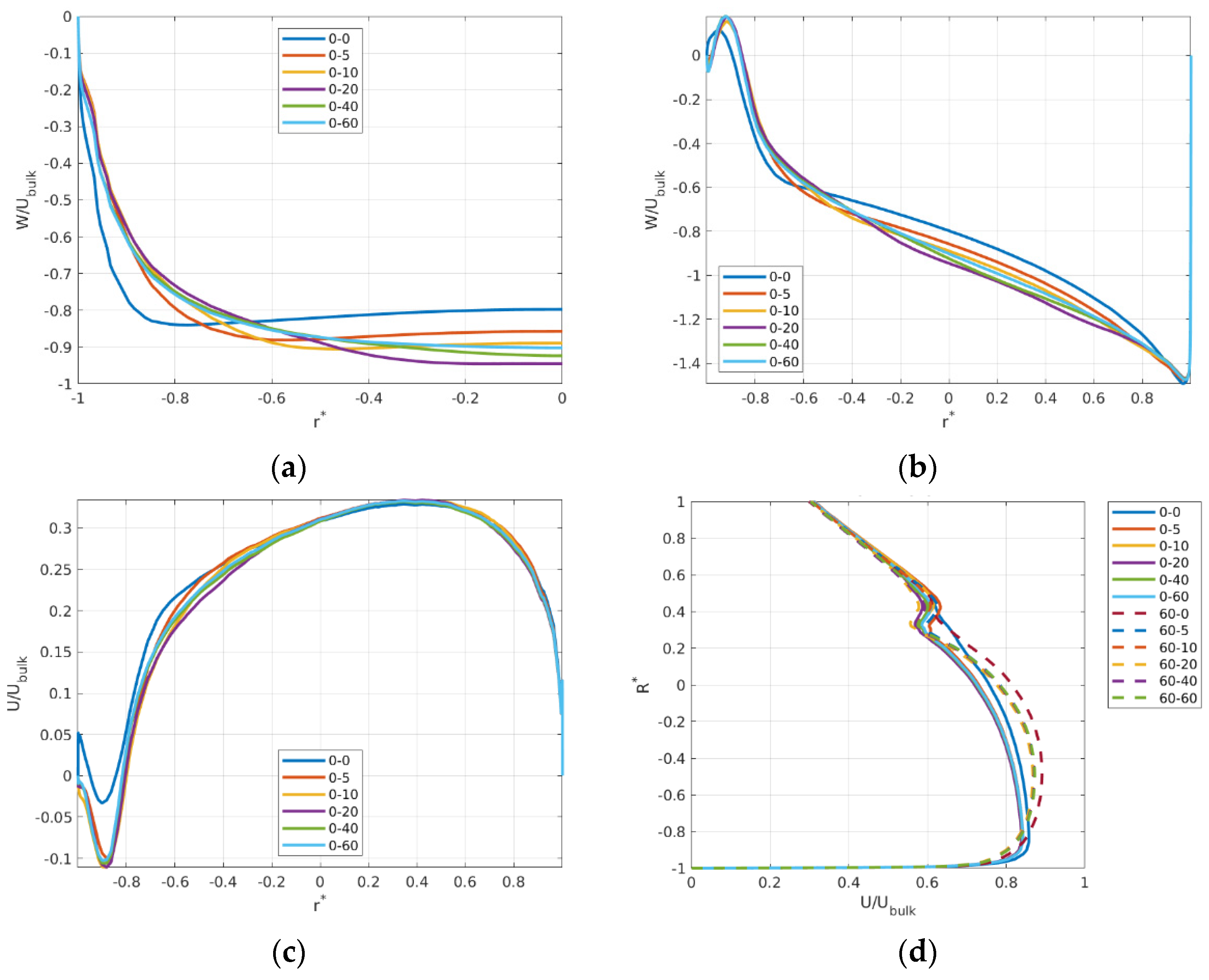
4.1. Profiles of Mean Temperature and Velocity

Profiles of $T^{*}$, $U/U_{bulk}$, and $W/U_{bulk}$ are compared in Figure 7 and Figure 8. Figure 7 shows the profiles of $T^{*}$ 1 mm away from the wall for top, side, and bottom walls to match the positions of the thermocouples used in the OECD/NEA-Vattenfall T-junction Benchmark. The highest temperature at the top and side of the pipe is reached with a combination of ‘0-0’ and ‘60-0’, whereas cases ‘0-20’ and ‘60-20’ present the lowest values at the same locations.

Comparing the cases with uniformly distributed profiles at the main pipe with the cases with fully developed profiles at the main inlet, the overall values are slightly higher than the ones obtained with uniformly distributed BCs. At the top of the pipe (Figure 7a–c), the profiles suddenly drop due to the backflow of fluid and vortex breakdown in the proximity of the T-junction. Afterwards, $T^{*}$ increases for cases from ‘0-0’ to ‘0-10’ and from ‘60-0’ to ‘60-10’, up to 2$D$ downstream of the T-junction, before gradually decreasing again and flattening at around 10$D$. Cases from ‘0-20’ to ‘0-60’ and from ‘60-20’ to ‘60-60’ show a different behaviour downstream the recirculation region, with a very small increase, followed by a mild decline and a flattening at around 5$D$ downstream of the T-junction. Specifically, cases ‘0-60’ and ‘60-60’ present an almost constant value of $T^{*}$ after 2$D$.

Figure 8a shows the profiles of $W/U_{bulk}$ on the axis $x=$ 0 at a cross-section located just above the entrance region, i.e., at $z=0.07\mathrm{m}$, as indicated in Figure 6. Since the profiles are symmetric on this axis, only the values of half of the pipe are shown. From Figure 8a, the velocity is maximum at the sides of the pipe for cases ‘0-0’, ‘0-5’, and ‘0-10’, with the peaks gradually moving towards the centre of the pipe as the inlet flow profiles at the branch pipe becomes fully developed. Case ‘0-0’ presents the highest velocity at the sides of the pipe among all cases. Cases ‘0-20’, ‘0-40’, and ‘0-60’ show similar profiles, with the velocity peaking at the centre of the pipe. The fact that case ‘0-20’ presents the highest velocity among all cases could explain the lower value of $T^{*}$ at the top and side of the pipe for this case (see Figure 7b–d) as also suggested in [33].

Figure 8b shows the profiles of $W/U_{bulk}$ on $y=$ 0 at the same cross-section, i.e., at $z=0.07\mathrm{m}$. Close to the upstream edge, $W/U_{bulk}$ for the case ‘0-0’ is positive and directed upward. This upward motion is due to the recirculation and entrainment in the branch pipe related to the hovering vortex system. For cases from ‘0-5’ to ‘0-60’, however, $W/U_{bulk}$ is first directed downward before this upward motion. This means that a small recirculation and entrainment is present for these cases close to the upstream edge of the entrance region. Away from this edge, cases ‘0-0’, ‘0-5’, and ‘0-10’ present similar profiles. The lowest value of $W/U_{bulk}$ is observed for the case ‘0-0’ in the centre of the pipe. Cases ‘0-20’, ‘0-40’, and ‘0-60’ exhibit similar behaviours, with slightly higher values of $W/U_{bulk}$ at the centre of the pipe reached for the case ‘0-20’. The values of $U/U_{bulk}$ are also shown on the same axis and at the same cross-section in Figure 8c. From Figure 8c, close to the upstream edge, $U/U_{bulk}$ is first positive and directed downstream, and it then changes sign for case ‘0-0’, whereas for cases from ‘0-5’ to ‘0-60’ it is directed upstream. This is due again to the recirculation and entrainment related to the hovering vortex system.

The vertical profiles of $U/U_{bulk}$ are presented in Figure 8d for all cases at a cross-section at $x/D=0$. The upper half of the pipe is not influenced by the inlet flow profiles at the main inlet at this location and only the profiles on the lower half present differences. Specifically, in cases from ‘0-5’ to ‘0-60’ the velocity profile is much flatter and the gradient at the shear-layer jet-main flow seems lower compared with the cases from ‘60-5’ to ‘60-60’. The values of $U/U_{bulk}$ for cases ‘0-0’ and ‘60-0’ are instead more uniform for the whole pipe cross-section. Overall, cases with fully developed BCs at the main inlet present slightly higher values of $U/U_{bulk}$ in the lower half of the pipe which might explain the less strong recirculation and mixing observed downstream of the T-junction, resulting, therefore, in slightly higher distribution of $T^{*}$ compared with the respective cases with uniformly distributed BCs at the main inlet, Figure 7.

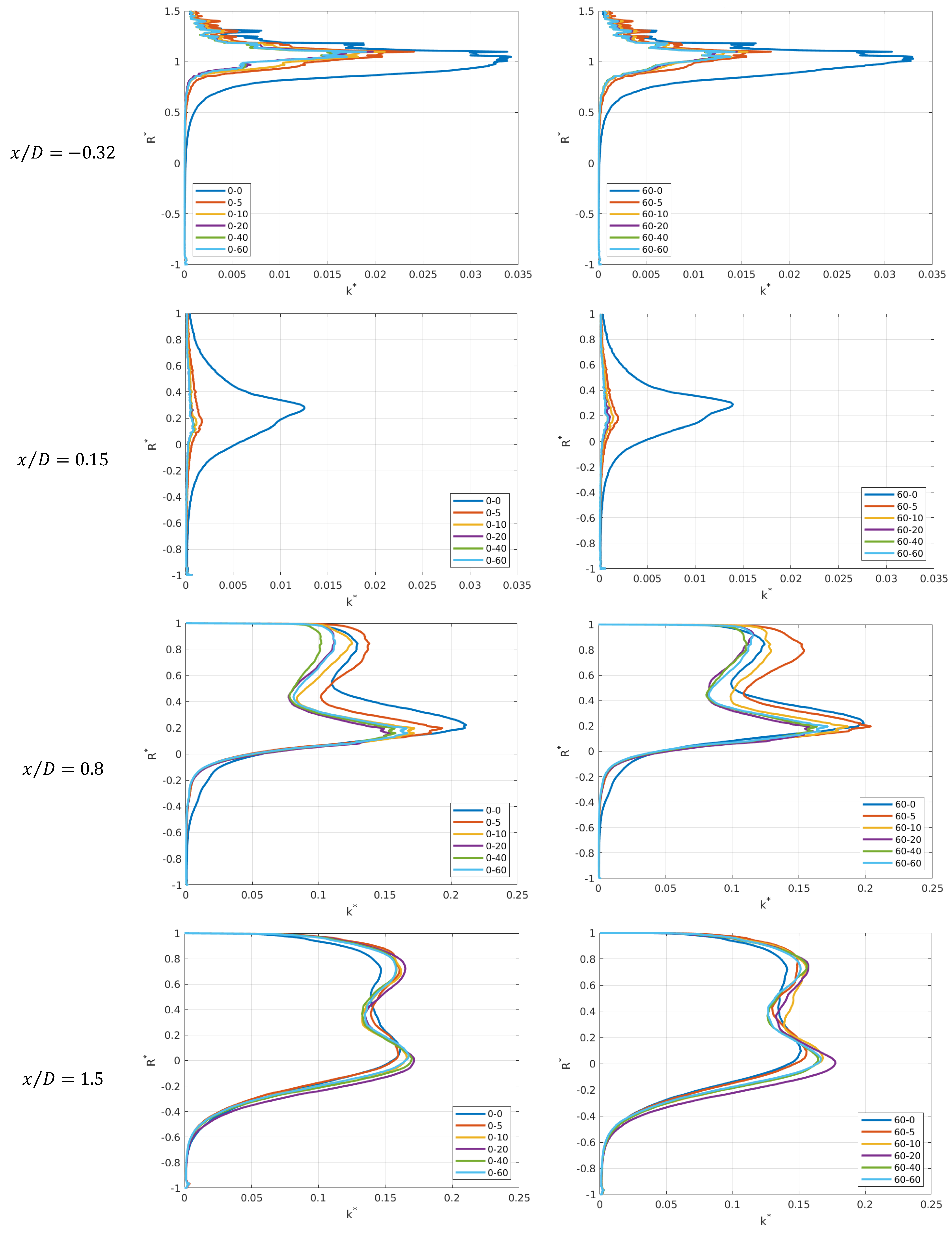
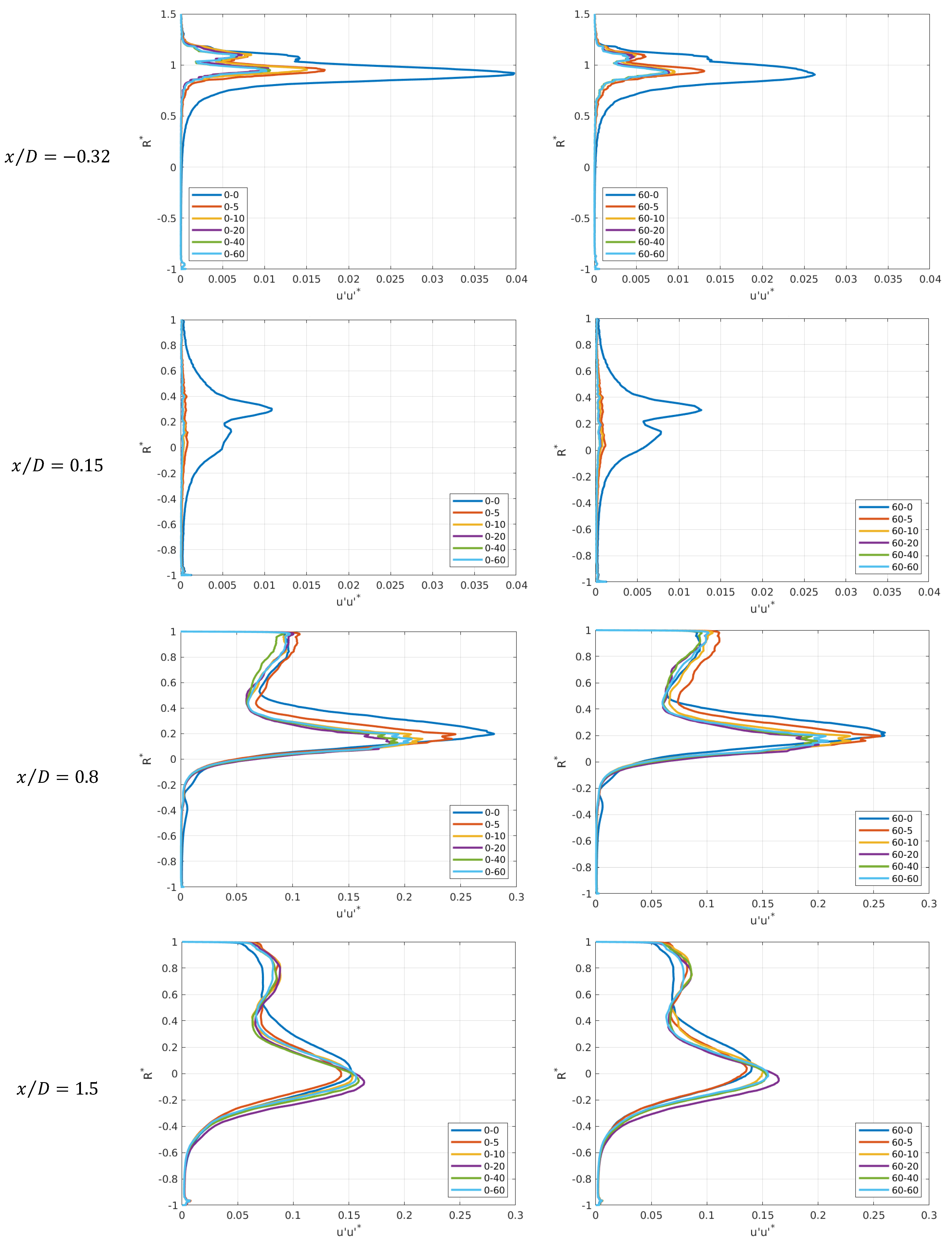
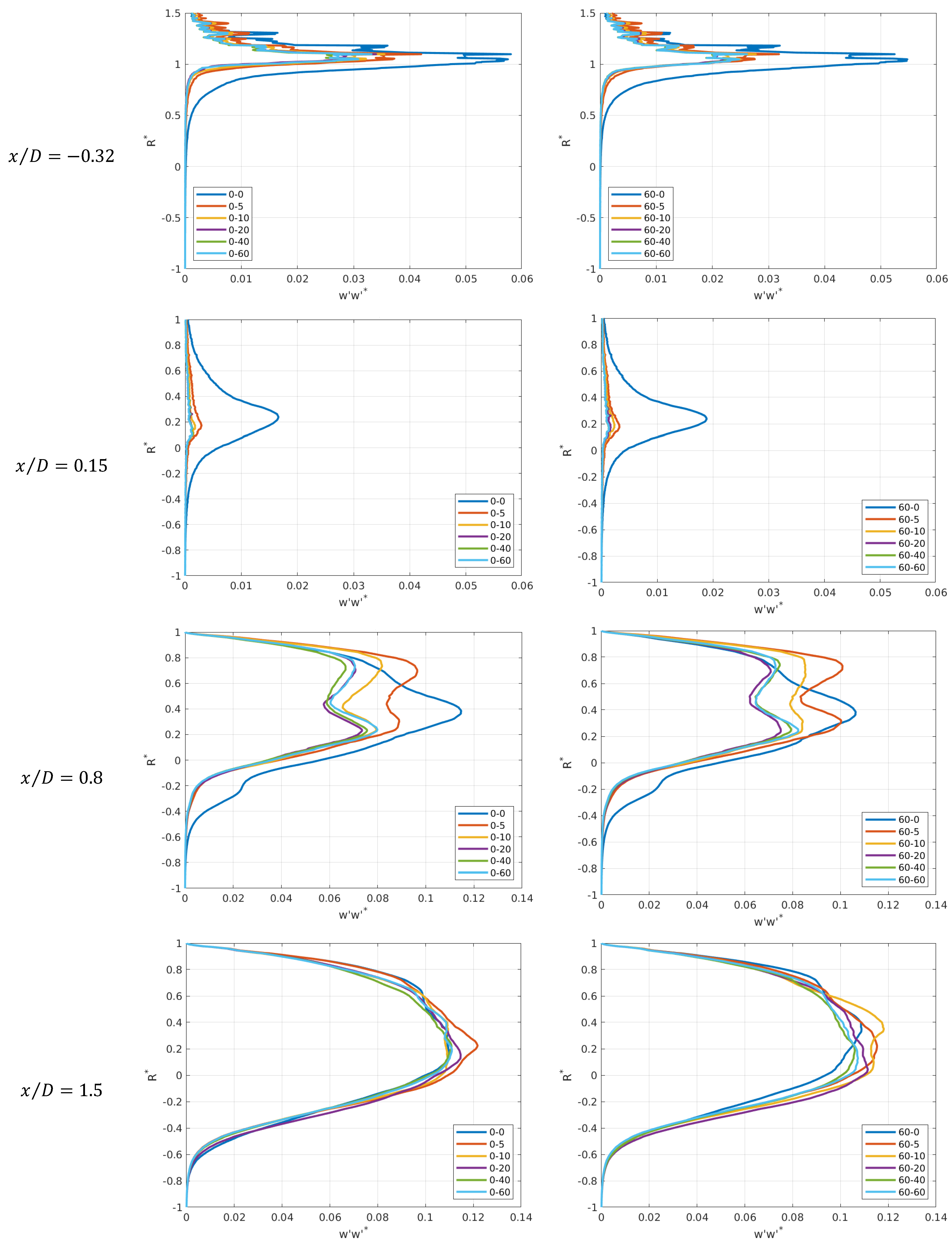
4.2. Effects of Different Inlet Flow Profiles on Turbulent Quantities

Vertical profiles of $k^{*}$, $u^{\prime }{u^{\prime }}^{*}$, $v^{\prime }{v^{\prime }}^{*}$, and $w^{\prime }{w^{\prime }}^{*}$ are shown at different cross-sections along the computational domain from Figure 9, Figure 10, Figure 11 and Figure 12. Figure 9 shows a peak in the vertical profile of $k^{*}$ at $x/D=-0.32$ whose value is almost double in cases ‘0-0’ and ‘60-0’ compared with the others. The peaks are located in the branch pipe just above the jet entrance and correspond to the position of the hovering vortex system. This result agrees with the observation about the higher vorticity of the hovering vortex system for the cases ‘0-0’ and ‘60-0’ discussed in Section 4.3 (see also Figure 13). The plots of $k^{*}$ show peaks for these two cases also at $x/D=0.15$ at the shear-layer jet-main flow, whereas almost no peaks are present for the other cases. The profiles of $k^{*}$ in the recirculation region, $x/D=0.8$, show an ‘S’ shape in all cases. The peaks are located at the shear-layers, the one between the recirculation bubble and the jet and the other between the jet and main flow. Additionally, peaks at shear-layer formed between the jet and main flow are higher due to the development of the mixing layer at $x/D=0.8$. The S-shaped profile is also maintained at $x/D=1.5$ where the top peak corresponds instead to the CVP.

Normal stresses at the same locations are illustrated in Figure 10, Figure 11 and Figure 12. The profiles differ the most in the upstream region, e.g., $x/D=-0.32$, and at the jet entrance, e.g., $x/D=0.15$. In the upstream region, peaks of $u^{\prime }{u^{\prime }}^{*}$ and $w^{\prime }{w^{\prime }}^{*}$ are higher in cases ‘0-0’ and ‘60-0’. Also, uniformly distributed BCs at the main inlet led to higher $u^{\prime }{u^{\prime }}^{*}$ and $w^{\prime }{w^{\prime }}^{*}$, i.e., cases from ‘0-5’ to ‘0-60’. Values of $v^{\prime }{v^{\prime }}^{*}$ in this region are instead much lower compared with the values of the other normal stresses for all cases. Moving to the jet entrance region, e.g., $x/D=0.15$, only cases ‘0-0’ and ‘60-0’ exhibit peaks of $u^{\prime }{u^{\prime }}^{*}$ and $w^{\prime }{w^{\prime }}^{*}$, whereas values of $v^{\prime }{v^{\prime }}^{*}$ are still low for all cases. Higher values of the normal stresses can be found in the recirculation region and in the reattachment region. The profiles of the normal stresses at $x/D=0.8$ and $x/D=1.5$ are similar among the cases. Peaks of $u^{\prime }{u^{\prime }}^{*}$ can be found at the shear-layer jet-main flow, whereas peaks of $v^{\prime }{v^{\prime }}^{*}$ are located close to the top wall. The profiles of $w^{\prime }{w^{\prime }}^{*}$ at $x/D=0.8$ assume a saddle-like shape for cases from ‘0-5’ to ‘0-60’ and from ‘60-5’ to ‘60-60’. For cases ‘0-0’ and ‘60-0’ instead, the profiles of $w^{\prime }{w^{\prime }}^{*}$ at the same location assume a single-peak-shape. Further downstream at $x/D=1.5$, all cases present a maximum of $w^{\prime }{w^{\prime }}^{*}$ in correspondence of the CVP.

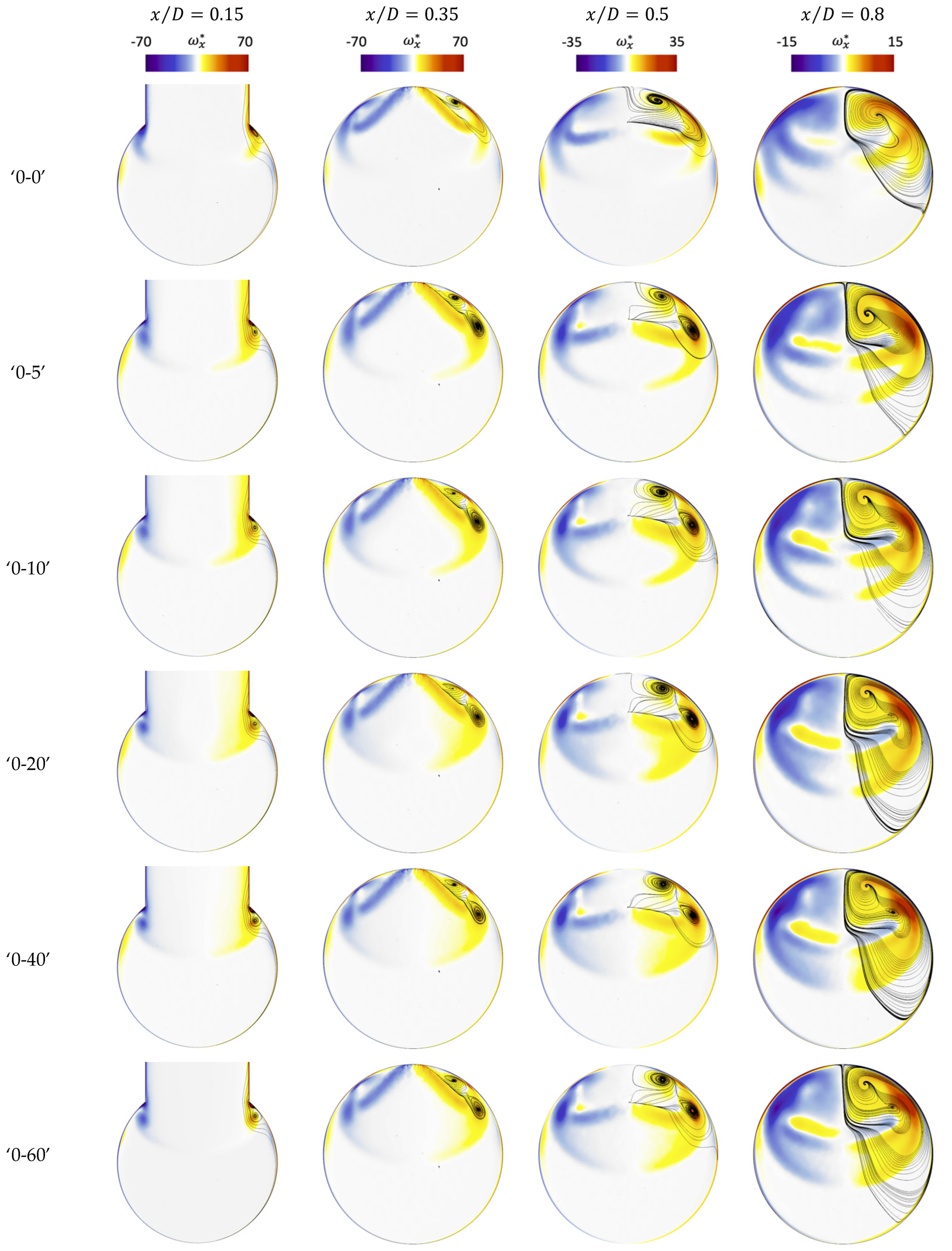
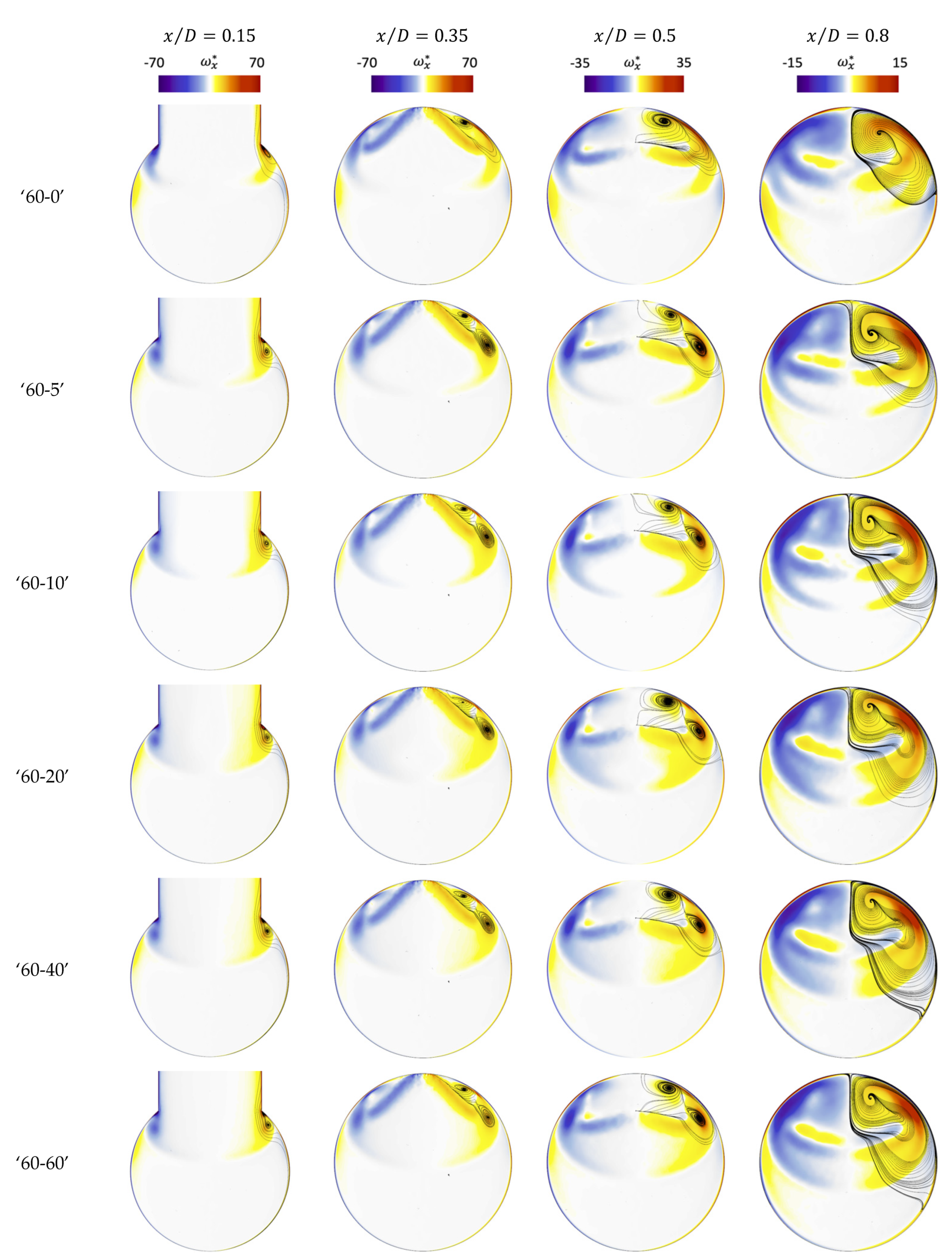
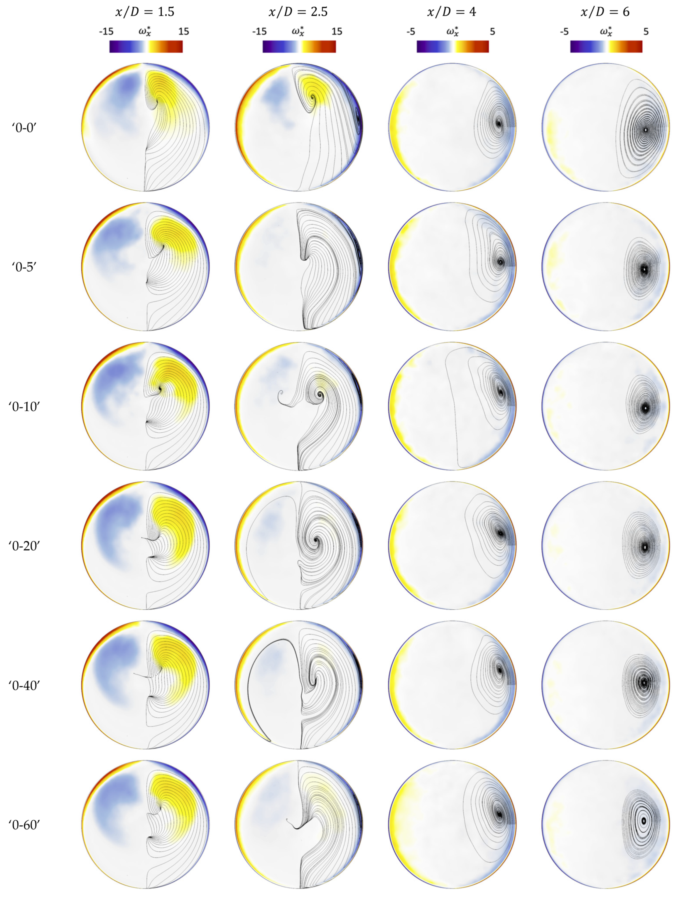
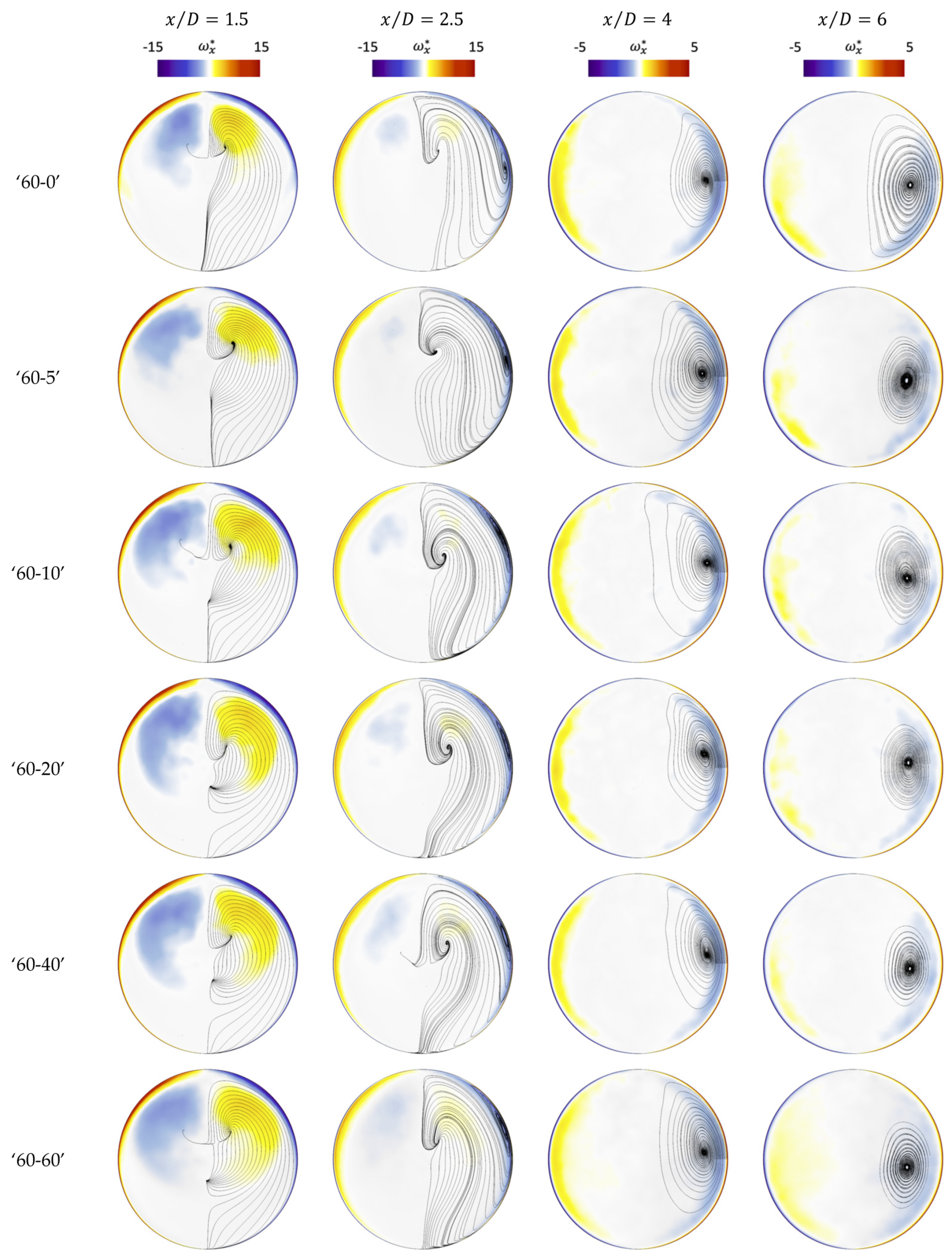
4.3. Effects of Different Inlet Flow Profiles on the Mean Flow Structure

The contours of ${\omega }_y^{*}$ and the streamline of the in-plane mean velocity, namely the velocity vector projected on the plane, are presented in Figure 13. These contours show the distribution of the horseshoe and hovering vortex systems among the different cases on the XZ symmetry plane. The vortical structure related to the hovering vortex and the recirculation region in the branch pipe, close to the upstream vertical wall, consists of a single vortex for cases ‘0-0’ and ‘0-60’ with associated higher values of ${\omega }_y^{*}$ compared with the other cases. Cases from ‘0-5’ to ‘0-60’ and ‘60-5’ to ‘60-60’ show instead an additional area of concentrated ${\omega }_y^{*}$ just above the jet entrance region that creates a double roll-up of the shear-layer between the jet-main flow. For these cases, the double roll-up structure seems to be induced by the horseshoe vortex that reaches the vertical wall of the branch pipe, pushing the fluid further away from the upstream edge of the branch pipe. In cases ‘0-0’ and ‘60-0’, the horseshoe vortex does not enter the branch pipe and remains instead closer to the main pipe wall, limiting its influence on the hovering vortex, which results in a single roll-up vortex. Consequently, the roll-up structure in cases ‘0-0’ and ‘60-0’ carries mainly hot water from the branch pipe and contributes less to the thermal mixing of the fluids (see Figure 7).

The vortical structure related to the horseshoe vortex and the recirculation region in the main pipe, close to the horizontal upper wall, consists also of a single vortex roll-up for cases ‘0-0’ and ‘0-60’ with associated higher values of ${\omega }_y^{*}$ compared with the other cases. For cases ‘0-20’, ‘0-40’, and ‘0-60’, additional vortex roll-ups appear at the upstream edge of the jet entrance. These roll-ups enhance the mixing locally due to the entrainment of fluid from the branch pipe in these vortical structures, which then result in a lower $T^{*}$ distribution as discussed in Section 4.1. Compared with cases with uniformly distributed BCs at the main inlet, i.e., from ‘0-5’ to ‘0-60’, the additional areas of ${\omega }_y^{*}$ seem smaller, resulting in an overall weaker double roll-up structure for the hovering vortex and horseshow vortex systems for cases with fully developed BCs at the main inlet, i.e., from ‘60-5’ to ‘60-60’. The thermal mixing associated with the horseshoe and hovering vortex system is lower in cases from ‘60-5’ to ‘60-60’ compared with cases from ‘0-5’ to ‘0-60’, producing overall higher $T^{*}$ distribution, which agrees with the discussion in Section 4.1.

Cross-sections located at $x/D=0.15$ and $x/D=0.35$ are selected for the jet entrance region. The contours of ${\omega }_x^{*}$ and the streamlines generated by the in-plane mean velocity are shown in Figure 14 and Figure 15. The streamlines are symmetric with respect to the z-axis and are shown for simplicity over half pipe cross-section. At $x/D=0.15$, two regions of concentrated streamwise vorticity with opposite sign, i.e., the primary counter-rotating vortex pair, located at the jet entrance at the sides of the branch pipe are observed. The primary vortex pair is still observed at the section $x/D=0.35$, where it starts to transition to two kidney-shaped regions. For cases with non-uniformly distributed BCs at the branch inlet, i.e., from ‘0-5’ to ‘0-60’ and from ‘60-5’ to ‘60-60’, the contours of ${\omega }_x^{*}$ at $x/D=0.15$ show additional regions of concentrated vorticity just below the jet entrance next to the main pipe wall. These additional regions represent the secondary counter-rotating vortex pair (Figure 14 and Figure 15). The presence of the secondary counter-rotating vortex pair indicates an earlier transition of the distribution of ${\omega }_x^{*}$ to the kidney-shaped compared with cases with uniformly distributed BCs. The double pairs of counter-rotating vortices, i.e., the primary and secondary vortex pairs, are maintained even further downstream at $x/D=0.35$. At this cross-section, the nested vortices embedded in the double pairs of counter-rotating vortices are also shown. Compared with the cases ‘0-0’ and ‘60-0’, the double pairs of counter-rotating vortices observed at $x/D=0.15$ improve the thermal mixing at the sides of the pipe and prevent hot fluid moving toward the wall. Specifically, the primary vortex pair improves the mixing at the top of the pipe, whereas the secondary vortex pair increases the mixing at the sides. Due to the lack of these double pairs in cases ‘0-0’ and ‘0-60’, the primary vortex pair carries only water from the branch pipe, resulting in a higher value of $T^{*}$ at the top of the pipe (see also discussion in Section 4.1).

Considering the effects of the inlet flow profiles at the main pipe, it can be observed that, overall, uniformly distributed BCs result in vortices with higher vorticity which increase the mixing locally and lead to lower values of $T^{*}$ across the cross-sections (see also discussion in Section 4.1). It is worth mentioning that the nested vortices are not observed for cases ‘0-0’ and ‘60-0’ at $x/D=0.35$.

Cross-sections located at $x/D=0.5$ and $x/D=0.8$ are chosen to show the flow structure in the recirculation region. The contours of ${\omega }_x^{*}$, Figure 14 and Figure 15, clearly show the nested vortex pair for all cases which deforms and finally splits the kidney-like shaped vorticity in each half plane. The secondary vortex pair in cases ‘0-0’ and ‘60-0’ is not as strong as the ones observed in the other cases. The nested vortex pair moves downwards and pushes the secondary vortex pair radially, at $x/D=0.5$, until the secondary vortex pair almost disappears at $x/D=0.8$. For cases from ‘0-5’ to ‘0-60’ and from ‘60-5’ to ‘60-60’ the secondary vortex pair is barely present at the sides of the pipe whereas the primary vortex pair occupies the upper part of the pipe cross-section. The resulting vortex structure at the end of the recirculation region represents the CVP which is the dominating flow structure up to almost 3$D$ downstream of the T-junction. The CVP mainly carries the flow from the side of the jet into the recirculation region, Figure 14 and Figure 15, resulting in a lower mixing quality in cases ‘0-0’ and ‘60-0’ when compared with the other cases (see also Section 4.1).

The reattachment region is characterized by the CVP and the second pair of vortices rotating in the opposite direction to the CVP. The second pair of vortices is induced by the upward motion of the main flow overcoming the blockage caused by the jet and the recirculation zone, Figure 16 and Figure 17. The contours of ${\omega }_x^{*}$ show that the CVP is still present at $x/D=1.5$, whereas it disappears at $x/D=4$, where only the second pair of vortices with opposite vorticity sign appears. The streamline contours show the presence of the CVP at cross-sections $x/D=1.5$ and $x/D=2.5$ for all cases. The second pair of rotating vortices are also evident at $x/D=2.5$ for cases ‘0-0’ and ‘60-0’. On the other hand, this pair is still weak for cases from ‘0-5’ to ‘0-60’ and from ‘60-5’ to ‘60-60’. Cross-sections $x/D=4$ and $x/D=6$ show the development of the second pair of rotating vortices further downstream as it moves towards the centre of the pipe.

The resulting vortex structures for the upstream region, the jet entrance and the recirculation region are shown in Figure 18 and Figure 19. These vortical structures are extracted with the vortex core option available in STAR-CCM+ [45,46,47]. These vortex lines, shown in black in Figure 18 and Figure 19, are then used as a source to generate the streamlines of mean velocity which are coloured by $T^{*}$. From these figures, it is possible to clearly visualise the vortical structures associated with the horseshoe and hovering vortex systems, the vortices generated by the interaction at the shear-layer jet-main flow in the entrance region, the flow reversal in the recirculation region, and the CVP which dominates the region further downstream. For all cases, the phenomena of vortex breakdown can be observed just below the downstream edge of the entrance region, which agrees with the observations regarding the distribution of ${\omega }_x^{*}$ in the pipe cross-sections and the nested vortex pair (see Figure 14 and Figure 15). When the crossflow from the main pipe meets the jet from the branch pipe, it flows around the jet and goes into the recirculation region, i.e., in the wake region in front of the jet, and due to recirculation and flow reversal, it is pushed back toward the jet entrance region. From here, it flows downstream and follows the curvature of the jet just below the recirculation region.

For cases from ‘0-5’ to ‘0-60’ and from ‘60-5’ to ‘60-60’ (Figure 18 and Figure 19), the vortex core lines of the vortical structures in the recirculation area, shown with black lines, suddenly bend downwards at the end of the recirculation regions. This results in the CVP moving downward as well, leaving space for the streamlines originated from the horseshoe vortex in the upstream region to go around the jet and upwards, close to the top wall. This motion allows a larger portion of the colder fluid from the upstream region to be entrained in the recirculation region, flows back to the jet entrance, and finally follows the curvature of the jet just below the recirculation region, similarly to what happens with the vortex breakdown phenomenon. The resulting temperature distribution in these cases is therefore lower compared with cases ‘0-0’ and ‘60-0’ due to the improved mixing in the recirculation region, as shown in ref. [33,34,35,37,38]. The reason of the different configuration of the vortical structures in the recirculation region among the cases can be attributed to the momentum of the jet. In ref. [33], it is shown that fully developed BCs at the branch produce higher momentum at the centre of the branch pipe compared with uniformly distributed BCs (see also Figure 8a). On the other hand, uniformly distributed BCs at the branch inlet result in higher momentum at the sides of the branch pipe compared with fully developed BCs (Figure 8a). This can be interpreted as a jet of a smaller cross-section when using fully developed BCs at the branch inlet, which allows more space for cold fluid to flow around the jet itself (see also Figure 18 and Figure 19 top plan views).

It must be pointed out that the streamlines originated from the vortex systems in the upstream region for cases with fully developed BCs at the main inlet, Figure 19, do not show any entrainment of cold fluid in the recirculation region. This is because the vorticity related to the horseshoe and hovering vortex is lower compared with cases with uniformly distributed BCs at the main inlet as shown from the ${\omega }_y^{*}$ distribution in the cross-sections (see Figure 13). The vortex core algorithm can filter weaker lines which is why they are not shown in Figure 19. Another consequence of the different momentum distribution is that the streamlines originated in the hovering vortex systems join with the vortical structure formed at the shear-layer jet-main flow in the entrance region. It is reasonable to claim, according to Figure 14 and Figure 15, that this results in the predominant primary vortex pair and a delayed formation of the secondary vortex pair for cases ‘0-0’ and ‘60-0’ compared with the other cases. This could explain the two regions of concentrated ${\omega }_x^{*}$ shown in the cross-sections in the jet entrance region for cases ‘0-0’ and ‘60-0’ and the double pairs of counter-rotating vortices structure observed instead for cases from ‘0-5’ to ‘0-60’ and from ‘60-5’ to ‘60-60’.

4.4. Effects of Different Inlet Flow Profiles on Transient Flow Behaviours

Figure 20 shows a snapshot in time of the time-dependent normalised temperature for cases ‘0-0’, ‘0-60’, ‘60-0’, and ‘60-60’. Videos of over 1 s of simulation time are available in (https://doi.org/10.5281/zenodo.7299325). As discussed in ref. [33], it can be observed that there are similarities between the pair ‘0-0’ and ‘60-0’, and the pair ‘0-60’ and ‘60-60’, see Figure 20. More specifically, it is possible to identify instabilities such as Kelvin-Helmholtz instabilities at the shear-layer jet-main flow on the XZ symmetry plane for cases ‘0-0’ and ‘60-0’ (see Figure 20a,b). These instabilities are periodic and seem to start at the upstream wall of the branch pipe with the shear-layer roll-up induced possibly by the horseshoe and hovering vortex systems and entrainment of flow from the main pipe.

The shear-layer roll-up is also observed on the cross-sections close to the jet entrance region where it resembles a mushroom-like eddy (also observed in T-junction flow [48]). It seems this might be originated by the vorticity generated by the fluid flowing around the jet. The frequency of this roll-up is the same as the Kelvin-Helmholtz instabilities on the symmetry plane. For cases ‘0-60’ and ‘60-60’, the Kelvin-Helmholtz instabilities on the symmetry plane are not witnessed (see Figure 20c,d). However, periodical oscillations can be observed at the edges of the jet just below the jet entrance region. Just downstream of the entrance region, hot fluid from the jet edges start to shed upward and inward toward the recirculation bubble. Further downstream, this becomes more chaotic and resembles large roll-up vortices.

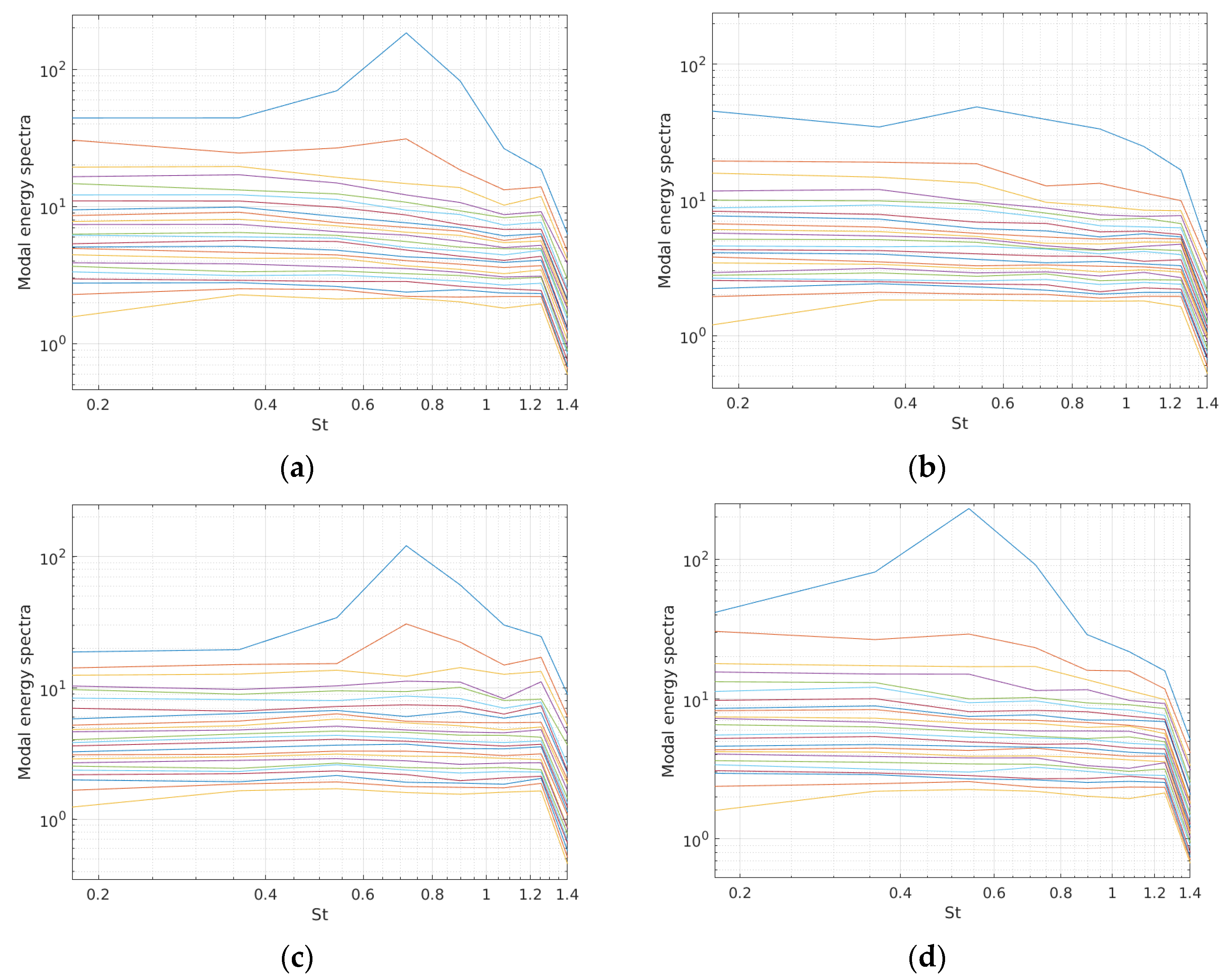
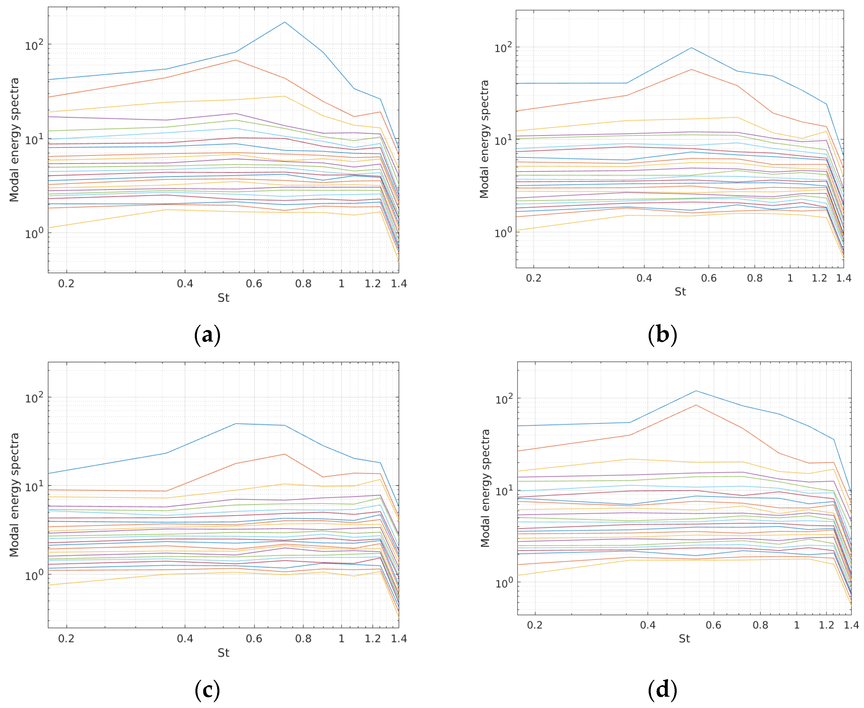
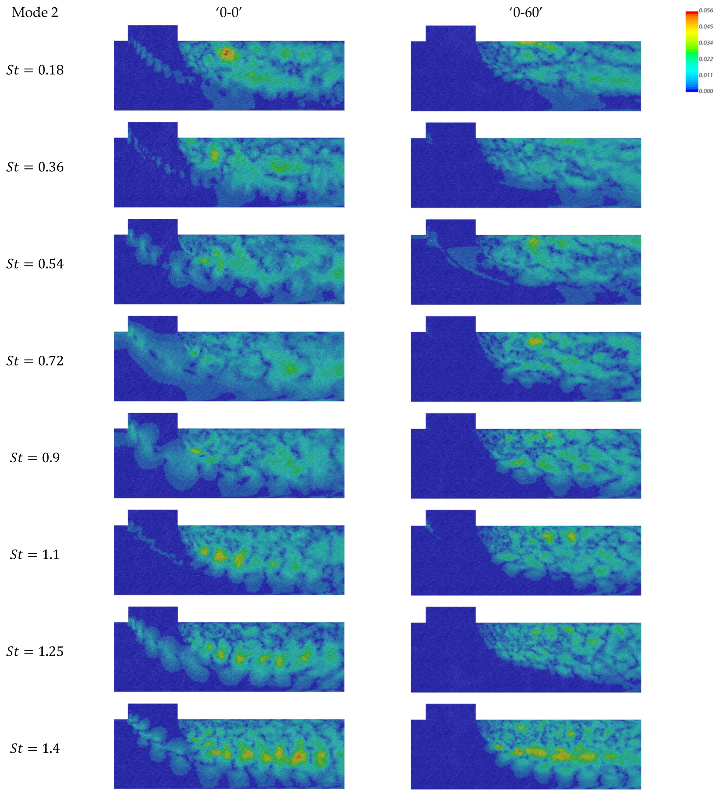
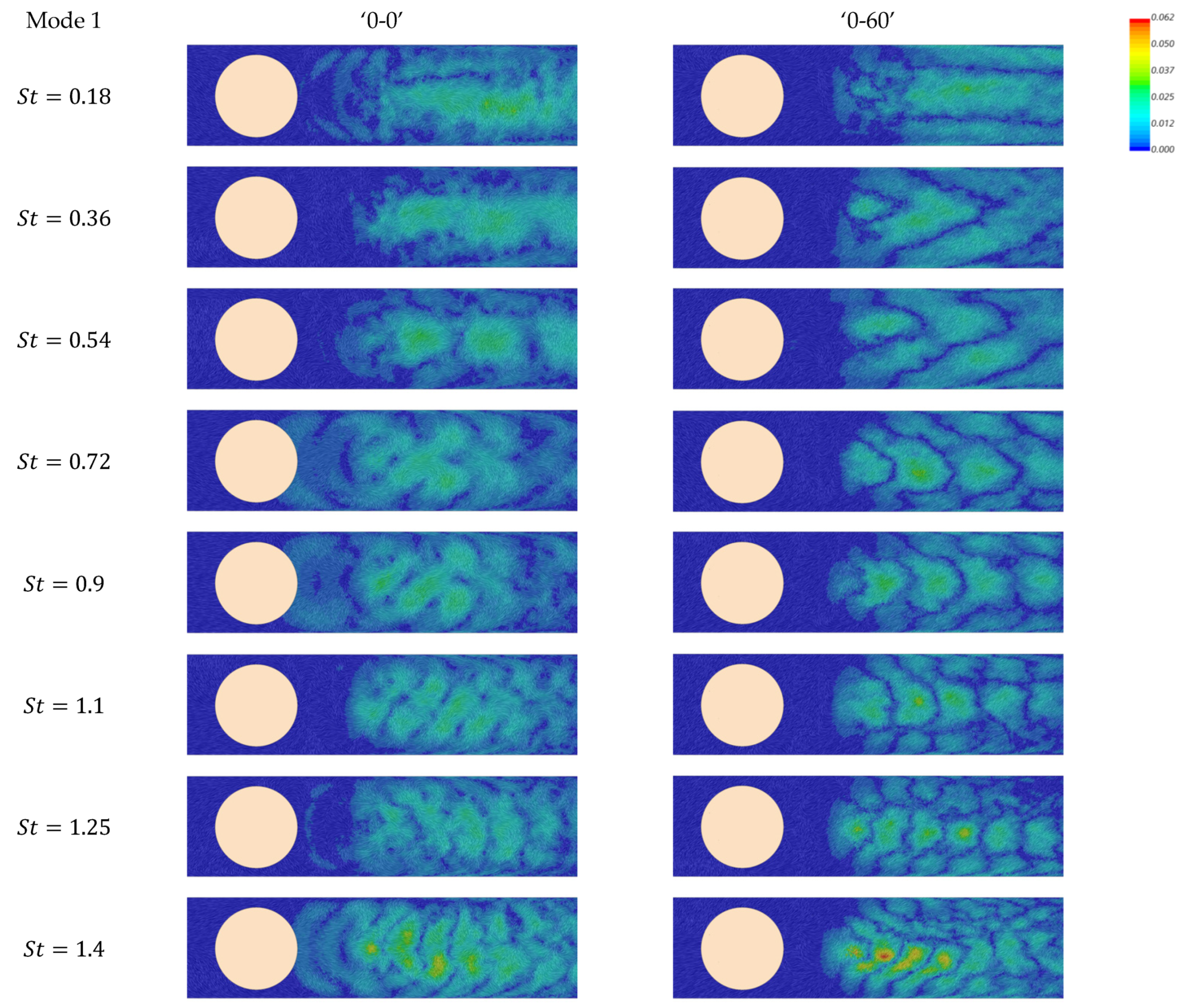
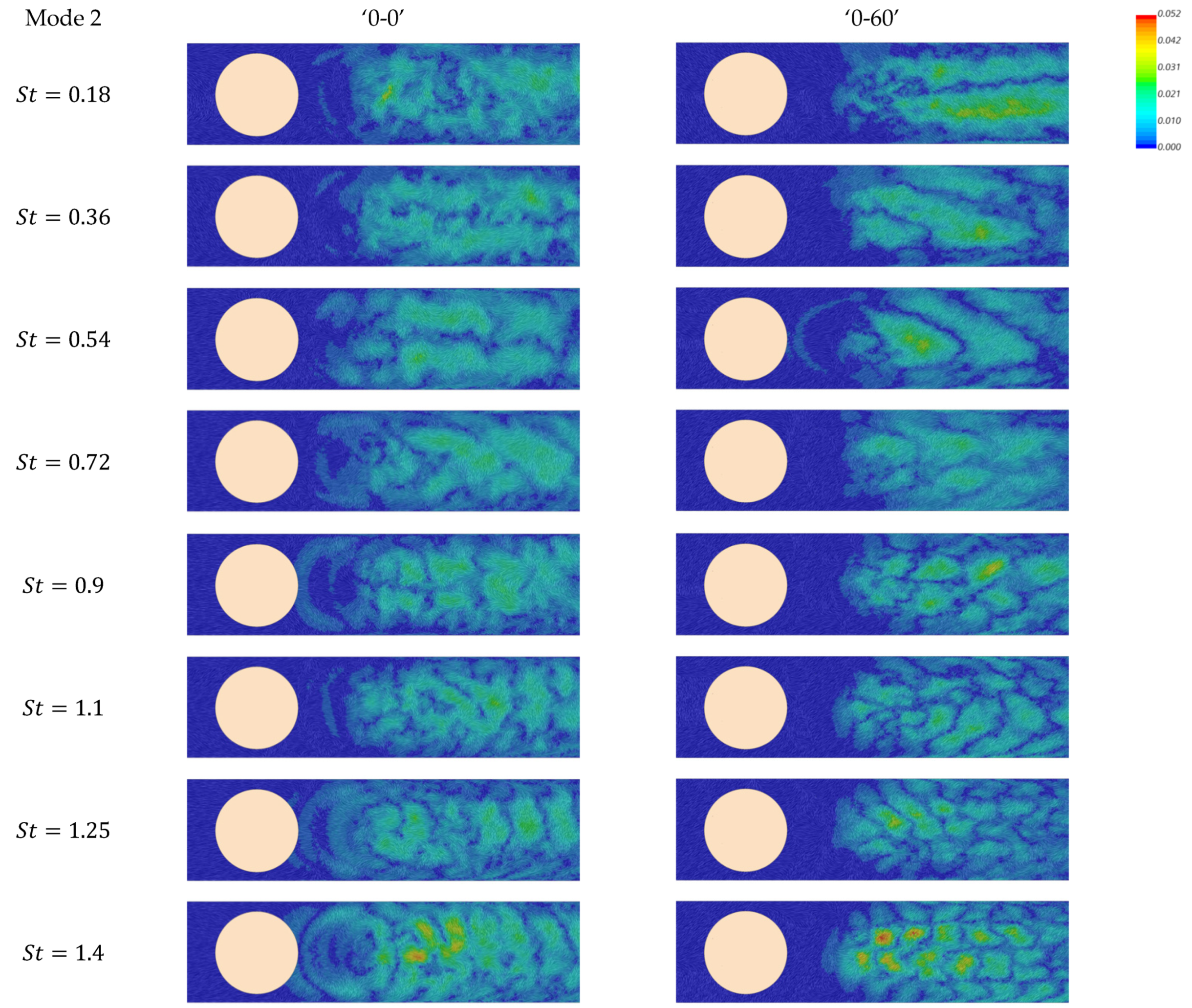
4.4.1. Spectral Proper Orthogonal Decomposition (SPOD) Analysis

The SPOD analysis [49], applied to the velocity field is used to extract and analyse the coherent structures of the flow. As opposed to standard POD, the modes calculated with SPOD are orthogonal both in space and time. Therefore, this makes SPOD a better method to extract spatial-temporal structures in the data [50]. The time-history of the velocity signal is recorded with a frequency of 0.05 s for a total of 10 s, which gives 200 snapshots overall. Since the transient behaviour is quite similar for the pair ‘0-0’ and ‘60-0’, and the pair ‘0-60’ and ‘60-60’, only the results of the cases ‘0-0’ and ‘0-60’ are shown.

The MATLAB spod.m subfunction [51,52] is used for the SPOD analysis with 16 snapshots analysed per block and a block overlap of 8 snapshots. The total number of blocks is 24, which gives a total of 24 modes and 9 frequencies. The frequency $f$ is normalised by $U_{bulk}$ and the diameter of the main pipe, $D$, using the Strouhal number $St$ defined as:

$$St=fD/U_{bulk}.$$

(9)

The modes energy for cases ‘0-0’ and ‘0-60’ obtained for the velocity signal at the symmetry planes XZ and XY are shown in Figure 21 and Figure 22. The first and second modes contain most of the energy. Therefore, only the vector contours of the first two modes are shown on the XZ and XY symmetry planes. The dominant frequency modes for the case ‘0-0’ is of $St=$ 0.72 for the velocity on the XZ symmetry plane and in the range 0.54–0.72 for velocity on the XY plane, whereas it is of 0.54 for the velocity on the XZ and XY planes for case ‘0-60’.

Figure 23 and Figure 24 present contour plots of the first and second modes on the XZ plane of the x- and z-component of velocity coloured by the mode’s magnitude. Figure 23 reveals several periodical vortical structures at the shear-layer jet-main flow in the entrance region for case ‘0-0’ at all frequencies, which are instead not present for case ‘0-60’. For the case ‘0-0’, at low $St$ numbers, very small vortices start to shed from the upstream edge of the jet entrance and follow the jet curve downstream the T-junction. They seem to extend for the entire thickness of the mixing layer and therefore can be generated by the shear-layer between the jet and the main flow. At higher $St$ number, the vortex shedding from the upstream edge becomes bigger and more aligned along the jet curve.

From the position of the most upstream vortex, for the case ‘0-0’, it seems that the vortex shedding at $St=$ 0.36 is originated in the branch pipe and the ones observed up to $St=$ 0.72 are generated by the horseshoe vortex and hovering vortex systems. At higher $St$ numbers, vortex pairing appears at both lower and upper jet shear-layers and originates once again at the upstream edge of the branch pipe. However, for the case ‘0-60’, larger alternating regions, with respect to the x-direction, can be observed at low $St$ number. These seem not to be originated at the upstream corner but seem to come instead from the downstream edge. Larger vortical structures are observed at around $St=$ 0.54 at the upper shear-layer between jet-recirculation bubble. Moving toward higher values of $St$, these large vortical structures move downwards and double-vortex are seen at the shear-layer jet-main flow. Finally, large vortices can be seen downstream the recirculation region periodically organised along the shear-layer jet-main flow. The second mode contour plots are similar to the ones related to the first mode for both cases and do not show additional structures, and it is shown for completeness in Figure 24.

Figure 25 and Figure 26 present contour plots of the first mode for the x- and y-components of velocity on the XY plane. From Figure 25, at low $St$, small and non-ordinate vortical structures located at the sides of the pipe can be observed. These structures seem to be originated by the interaction of the shear-layer between the jet and the main flow moving at the sides of the incoming jet. At $St=$ 0.72, bigger vortices originate close to the T-junction and are symmetrically located with respect to the y-axis. This double-vortex structure is periodically repeated along the x-axis. For $St>$ 1.25, an additional vortex is formed on the symmetry axis, forming a three-vortex structure arranged on a semi-circular line that is periodically repeated along the x-axis. For the case ‘0-60’, no vortical structures can be observed along the x-axis. For this case, regions of high mode magnitude can be observed alternating along the y-axis at low $St$ and along the x-axis at medium and high $St$.

The contour plots of the second mode for the case ‘0-0’ show an alternating behaviour along the y-axis for low $St$ (up to $St=$ 0.72), which is not seen in the first mode (Figure 26). This is also observed to a lesser extent in case ‘0-60’. The distribution of these regions and the symmetry with respect to the y-axis might suggest that this alternating behaviour could be attributed to the CVP and the second pair of vortices, which rotates in the opposite direction to the CVP and are created by the upward motion of the main flow past the recirculation region. In Section 4.3, it was pointed out that this second pair of vortices has higher vorticity for cases with uniformly distributed BCs at the branch inlet compared with the other cases, which might explain the weaker alternating structure observed for the second mode of case ‘0-60’.

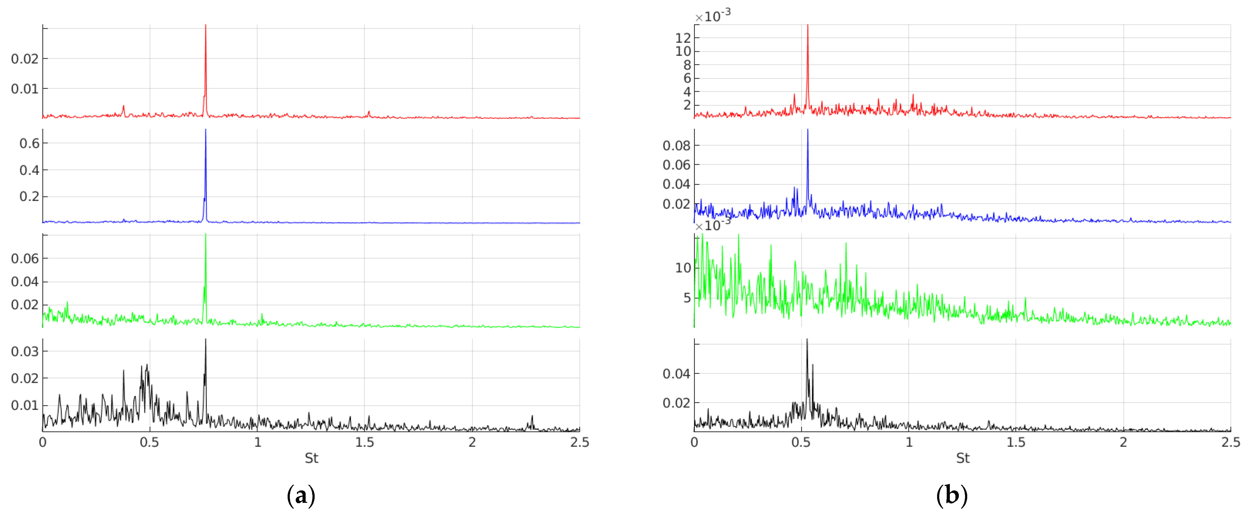
4.4.2. Power Spectral Density (PSD) Analysis

PSD analysis is used in this study to assess the time-history of the streamwise velocity signal and identify the dominant frequency modes in the flow. PSD contour plots of the streamwise velocity component are computed at cross-section $x/D=1.6$ for different points, as shown in Figure 6. For the sake of simplicity, only the results of cases ‘0-0’ and ‘0-60’ are presented. For the case ‘0-0’, the PSD contour plots of the streamwise velocity at cross-section $x/D=1.6$ show a distinct peak at around $St=$ 0.7 for all cross-sectional positions (see Figure 27). The vortical structure associated with a $St$ value of 0.7 comes from the interaction horseshoe-hovering vortex upstream the junction, as shown in Figure 23. The converted oscillation frequency related to $St=$ 0.7 is around 5 Hz which is in the range of concern for thermal fatigue [53]. In [33], it is shown that cases with uniformly distributed BCs at the branch inlet, i.e., ‘0-0’ and ‘60-0’, present peaks at around 5 Hz close to the top and side wall, which are not observed for cases with fully developed BCs at the branch inlet (cases ‘0-60’ and ‘60-60’). This might indicate that the vortical structures observed at this frequency are responsible for the higher temperature distribution at the top wall as well as for the oscillation in temperature for cases ‘0-0’ and ‘60-0’.

For the case ‘0-60’, no peaks are present at the upper half of the pipe, whereas peaks appear at the centre of the pipe and in the lower half of the pipe, for $St$ between 0.4 and 0.5 (see Figure 27). These peaks can also be observed at the left side of the pipe. The frequencies related to $St=$ 0.4 and 0.5 are between 2 and 3 Hz and are again in the range of concern for thermal fatigue. Peaks in the same range of frequencies at the sides of the pipe are also observed in other studies [31] and found to be linked to the spanwise oscillations in the temperature signal similar to vortex shedding behind a solid body. Peaks at these frequencies are also observed in the PSD plots of temperature for cases ‘0-60’ and ‘60-60’ at the sides of the pipe, as shown in [33]. Therefore, it can be said that the oscillations in streamwise velocity occurring in the lower half of the pipe and at the centre of the pipe might be responsible for oscillations in temperature close to the side wall. From Figure 27a, it can be observed that case ‘0-0’ also shows a peak at $St=$ 0.5 at the left side, which can cause the oscillations in the temperature at the sides of the wall at this cross-section, also observed in [33]. Higher frequency modes peaks can be found only for the case ‘0-0’ at around $St=$ 1.4, namely, frequency of 10 Hz, in the lower half of the pipe, Figure 27. This corresponds to the large structure observed in the SPOD modes at XZ symmetry plane and are not seen for the case ‘0-60’ (Figure 23). A peak at this frequency, i.e., 10 Hz, is also observed in the PSD of temperature at the sides of the pipe for these two cases [33]. This might be due to the shear-layer roll-up observed in the cross-section which is also shown in the first mode of the SPOD at XY symmetry plane (Figure 25).

5. Conclusions

This paper analyses the effects of different inlet flow profiles on thermal mixing within a T-junction. The flow domain is modelled using the IDDES-SST turbulence model implemented within the commercial CFD software STAR-CCM+ 2020.1.1. Different combinations of inlet flow profiles are considered. These inlet flow profiles are related to different stages in the flow entry region and range from uniformly distributed to fully developed. The influence of the inlet flow profiles on the mean and transient flow structures is assessed. The mean flow structures in the T-junction can be characterised by the horseshoe and hovering vortex systems in the upstream region, the primary, secondary and nested vortex pairs generated in the entrance and recirculation regions, as well as the CVP and the second pair of vortices in the reattachment region. The transient flow structures can be summarised in the Kelvin-Helmholtz instabilities, shear-layer roll-up, and Karman vortex street phenomena.

It is shown that the hovering and horseshoe vortex systems present higher vorticity for cases with uniformly distributed BCs at the main inlet compared with the ones with fully developed BCs at the main inlet. The use of fully developed BCs at the main inlet causes more cold fluid to be entrained in the recirculation zone in the branch pipe, and hence improves the thermal mixing in the branch pipe. For cases with non-uniformly distributed BCs at the branch inlet, the hovering vortex assumes a double roll-up shape as opposed to a single roll-up in cases with uniformly distributed BCs at the branch inlet. The double roll-up shape also increases the mixing in the branch pipe, resulting in a lower mean temperature distribution. In the jet entrance and recirculation regions, the appearance of the secondary vortex pair and the nested vortex pair is delayed for cases with uniformly distributed BCs at the branch inlet. This delay results in a lower thermal mixing and a higher mean temperature distribution in cases with uniformly distributed BCs at the branch inlet compared with the other cases. In the reattachment region, the CVP and the second pair of vortices are also different among the cases. Specifically, for cases with uniformly distributed BCs at the branch inlet the CVP and the second pair of vortices present higher vorticity compared with the other cases.

The SPOD analysis revealed a series of shear-layer roll-ups and Kelvin-Helmholtz instabilities originated from the shear-layer jet-main flow and the hovering and horseshoe systems for cases with uniformly distributed BCs at the branch inlet. Shear-layer roll-ups are also observed at the shear-layer jet-recirculation bubble for all cases. The dominant frequency modes observed in the PSD plots are in the range of concern for high cycle thermal fatigue and seem to be affected by the different inlet flow profiles used. For cases with uniformly distributed BCs at the branch inlet, the dominant frequency mode is at $St$ of around 0.7, which corresponds to a frequency of 5 Hz. In a previous study, this was shown to be the predominant frequency of the temperature near the top and sides wall for cases with uniformly distributed BCs at the branch inlet. For the other cases, the dominant frequency mode is at $St$ between 0.4 and 0.5, which is equivalent to 2–3 Hz, and same dominant frequencies were found for the temperature close to the side wall for cases with fully developed BCs at the branch inlet.

References

1. Kim, J.H.; Roidt, R.M.; Deardorff, A.F. Thermal stratification and reactor piping integrity. Nucl. Eng. Des. 1993, 139, 83–95. [Google Scholar] [CrossRef]
2. Jawad, M.H. Stress in ASME Pressure Vessels, Boilers, and Nuclear Components; Wiley-ASME Press Series; 2017. Available online: https://www.wiley.com/en-ae/Stress+in+ASME+Pressure+Vessels,+Boilers,+and+Nuclear+Components-p-9781119259282 (accessed on 10 October 2022).
3. Radu, V. Stochastic modelling of fatigue crack growth. In Applied Condition Monitoring Volume 1; Springer: Cham, Switzerland, 2015. [Google Scholar]
4. Weronski, A.; Hejwowski, T. Thermal Fatigue of Metals; Marcel Dekker: New York, NY, USA, 1991. [Google Scholar]
5. Sohn, H.; Yang, J.; Lee, H.; Park, B. 20—Sensing Solutions for Assessing and Monitoring of Nuclear Power Plants (NPPs); Woodhead Publishing: Sawston, UK, 2014; pp. 605–637. [Google Scholar] [CrossRef]
6. Brunings, J. LMFBR Thermal-Striping Evaluation; United States, 1982. Available online: https://www.osti.gov/servlets/purl/6887039 (accessed on 10 October 2022).
7. Jones, I.S. Thermal striping fatigue damage in multiple edge-cracked geometries. Fatigue Fract. Eng. Mater. Struct. 2006, 29, 123–134. [Google Scholar] [CrossRef]
8. Gelineau, O.; Sperandio, M.; Martin, P.; Ricard, J.B.; Martin, L.; Bougault, A. Thermal Fluctuation Problems Encountered in LMFRs (IWGFR–90); International Atomic Energy Agency (IAEA): Vienna, Austria, 1994. [Google Scholar]
9. Gelineau, O.; Sperandio, M.; Simoneau, J.P.; Hamy, J.M.; Roubin, P.H.L. Thermomechanical and Thermohydraulic Analyses of a T-Junction Using Experimental Data (IAEA-TECDOC–1318); International Atomic Energy Agency (IAEA): Vienna, Austria, 2002. [Google Scholar]
10. Chapuliot, S.; Gourdin, C.; Payen, T.; Magnaud, J.; Monavon, A. Hydro-thermal-mechanical analysis of thermal fatigue in a mixing tee. Nucl. Eng. Des. 2005, 235, 575–596. [Google Scholar] [CrossRef]
11. Shah, V.N.; MacDonald, P.E. (Eds.) Aging and Life Extension of Major Light Water Reactor Components; Elsevier Science Publishers: Amsterdam, The Netherlands, 1993. [Google Scholar]
12. IAEA. Assessment and Management of Ageing of Major Nuclear Power Plant Components Important to Safety: Primary Piping in PWRs; IAEA-TECDOC 1361; IAEA: Vienna, Austria, 2003. [Google Scholar]
13. Bartmann, B.; Neikes, R.; Leweke, T.; Limberg, W.; Krause, E. Vortex Formation in a T-Junction; Tanida, Y., Miyashiro, H., Eds.; Springer: Berlin/Heidelberg, Germany, 1992; pp. 102–106. [Google Scholar] [CrossRef]
14. Perry, A.E.; Lim, T.T. Coherent structures in coflowing jets and wakes. J. Fluid Mech. 1978, 88, 451–463. [Google Scholar] [CrossRef]
15. Perry, A.E.; Tan, D.K.M. Simple three-dimensional vortex motions in coflowing jets and wakes. J. Fluid Mech. 1984, 141, 197–231. [Google Scholar] [CrossRef]
16. Andreopoulos, J. On the structure of jets in a crossflow. J. Fluid Mech. 1985, 157, 163–197. [Google Scholar] [CrossRef]
17. Andreopoulos, J.; Rodi, W. Experimental investigation of jets in a crossflow. J. Fluid Mech. 1984, 138, 93–127. [Google Scholar] [CrossRef]
18. Kelso, R.M.; Lim, T.T.; Perry, A.E. An experimental study of round jets in cross-flow. J. Fluid Mech. 1996, 306, 111–144. [Google Scholar] [CrossRef]
19. Fric, T.F.; Roshko, A. Vortical structure in the wake of a transverse jet. J. Fluid Mech. 1994, 279, 1–47. [Google Scholar] [CrossRef] [Green Version]
20. Brücker, C. Study of the three-dimensional flow in a T-junction using a dual-scanning method for three-dimensional scanning-particle-image velocimetry (3-D SPIV). Exp. Therm. Fluid Sci. 1997, 14, 35–44. [Google Scholar] [CrossRef]
21. Brucker, C.; Althaus, W. Study of vortex breakdown by particle tracking velocimetry (PTV). Exp. Fluids 1992, 13, 339–349. [Google Scholar] [CrossRef]
22. Abramovich, G.N. The Theory of Turbulent Jets; Schindel, L., Ed.; The MIT Press: Cambridge, MA, USA, 2003. [Google Scholar] [CrossRef]
23. Smith, B.L.; Mahaffy, J.H.; Angele, K.; Westin, J. Report of the OECD/NEA-Vattenfall T-Junction Benchmark Exercise; OECD: Paris, France, 2011; pp. 1–92. [Google Scholar]
24. Smith, B.; Mahaffy, J.; Angele, K. A CFD benchmarking exercise based on flow mixing in a T-junction. Nucl. Eng. Des. 2013, 264, 80–88. [Google Scholar] [CrossRef]
25. Braillard, O.; Howard, R.; Angele, K.; Shams, A.; Edh, N. Thermal mixing in a T-junction: Novel CFD-grade measurements of the fluctuating temperature in the solid wall. Nucl. Eng. Des. 2018, 330, 377–390. [Google Scholar] [CrossRef] [Green Version]
26. Shams, A.; Edh, N.; Angele, K.; Veber, P.; Howard, R.; Braillard, O.; Chapuliot, S.; Severac, E.; Karabaki, E.; Seichter, J.; et al. Synthesis of a CFD benchmarking exercise for a T-junction with wall. Nucl. Eng. Des. 2018, 330, 199–216. [Google Scholar] [CrossRef]
27. Westin, J.; Alavyoon, F.; Andersson, L.; Veber, P.; Henriksson, M.; Andersson, C. Experiments and Unsteady CFD-Calculations of Thermal Mixing in a T-Junction. In Proceedings of the OECD/NEA/IAEA Workshop on the Benchmarking of CFD Codes for Application to Nuclear Reactor Safety (CFD4NRS), Munich, Germany, 5–7 September 2006; pp. 1–15. [Google Scholar]
28. Westin, J.; Veber, P.; Andersson, L.; Mannetje, C.; Andersson, U.; Eriksson, J.; Henriksson, M.E.; Alavyoon, F.; Andersson, C. High-Cycle Thermal Fatigue in Mixing Tees: Large-Eddy Simulations Compared to a New Validation Experiment. In Proceedings of the 16th International Conference on Nuclear Engineering, Orlando, FL, USA, 11–15 May 2008; pp. 515–525. [Google Scholar] [CrossRef] [Green Version]
29. Odemark, Y.; Green, T.M.; Angele, K.; Westin, J.; Alavyoon, F.; Lundström, S. High-Cycle Thermal Fatigue in Mixing Tees: New Large-Eddy Simulations Validated Against New Data Obtained by PIV in the Vattenfall Experiment. In Proceedings of the 17th International Conference on Nuclear Engineering, Brussels, Belgium, 12–16 July 2009; pp. 775–785. [Google Scholar] [CrossRef]
30. Evrim, C.; Laurien, E. Large-Eddy Simulation of turbulent thermal flow mixing in a vertical T-Junction configuration. Int. J. Therm. Sci. 2020, 150, 106231. [Google Scholar] [CrossRef]
31. Gritskevich, M.; Garbaruk, A.; Frank, T.; Menter, F. Investigation of the thermal mixing in a T-junction flow with different SRS approaches. Nucl. Eng. Des. 2014, 279, 83–90. [Google Scholar] [CrossRef]
32. Kang, D.G.; Na, H.; Lee, C.Y. Detached eddy simulation of turbulent and thermal mixing in a T-junction. Ann. Nucl. Energy 2019, 124, 245–256. [Google Scholar] [CrossRef]
33. Lampunio, L.; Duan, Y.; Eaton, M.D. The effect of inlet flow conditions upon thermal mixing and conjugate heat transfer within the wall of a T-Junction. Nucl. Eng. Des. 2021, 385, 111484. [Google Scholar] [CrossRef]
34. Lampunio, L.; Duan, Y.; Issa, R.; Eaton, M.D. Thermal Stripping Analysis in T-junctions with Different Entry Flow Profiles. In Proceedings of the Advances in Thermal Hydraulics 2020 (ATH2020), Palaiseau, France, 20–23 October 2020; pp. 895–906. [Google Scholar]
35. Lampunio, L.; Duan, Y.; Issa, R.; Eaton, M.D. Effects of inlet velocity profiles for thermal stripping phenomena in T-junctions. J. Phys. Conf. Ser. 2021, 2116, 12026. [Google Scholar] [CrossRef]
36. Schmidt, J. (Ed.) Process and Plant Safety Applying Computational Fluid Dynamics; Wiley-VCH Verlag & Co. KGaA: Weinheim, Germany, 2012. [Google Scholar]
37. Lampunio, L.; Duan, Y.; Eaton, M.D. Effects of different entry flow profiles on thermal striping in mixing T-junction. In Proceedings of the UK Heat Transfer Conference (UKHTC 2022), Manchester, UK, 3–5 April 2022. [Google Scholar]
38. Lampunio, L.; Duan, Y.; Eaton, M.D. Surrogate modelling and uncertainty quantification for the analysis of turbulent thermal mixing phenomena within a T-junction. In Proceedings of the 19th International Topical Meeting on Nuclear Reactor Thermal Hydraulics (NURETH-19), Brussels, Belgium, 6–11 March 2022. [Google Scholar]
39. Siemens Industries Digital Software. Simcenter STAR-CCM+, version 2020.1.1; Siemens: Waltham, MA, USA, 2020.
40. Gritskevich, M.S.; Garbaruk, A.V.; Schütze, J.; Menter, F.R. Development of DDES and IDDES formulations for the K-ω shear stress transport model. Flow Turbul. Combust. 2012, 88, 431–449. [Google Scholar] [CrossRef]
41. Menter, F.R. Two-equation eddy-viscosity turbulence models for engineering applications. AIAA J. 1994, 32, 1598–1605. [Google Scholar] [CrossRef] [Green Version]
42. Igarashi, M.; Tanaka, M.; Kawashima, S.; Kamide, H. Experimental Study on Fluid Mixing for Evaluation of Thermal Striping in T-Pipe Junction. In Proceedings of the 10th International Conference on Nuclear Engineering, Arlington, VA, USA, 14–18 April 2002; pp. 383–390. [Google Scholar] [CrossRef]
43. Kamide, H.; Igarashi, M.; Kawashima, S.; Kimura, N.; Hayashi, K. Study on mixing behavior in a tee piping and numerical analyses for evaluation of thermal striping. Nucl. Eng. Des. 2009, 239, 58–67. [Google Scholar] [CrossRef]
44. Foss, J.F. Interaction Region Phenomena for the Jet in a Crossflow Problem; SFB Report SFB 80/E/161; University Karlsruhe: Karlsruhe, Germany, 1984. [Google Scholar]
45. Sujudi, D.; Haimes, R. Identification of swirling flow in 3-D vector fields. In Proceedings of the AIAA 12th Computational Fluid Dynamics Conference, San Diego, CA, USA, 19–22 June 1995. [Google Scholar] [CrossRef] [Green Version]
46. Haimes, R.; Kenwright, D. On the velocity gradient tensor and fluid feature extraction. In Proceedings of the AIAA 14th Computational Fluid Dynamics Conference, Norfolk, VA, USA, 1–5 November 1999. [Google Scholar] [CrossRef]
47. Siemens Industries Digital Software. Simcenter STAR-CCM+ User Guide, version 2020.1.1; Siemens: Waltham, MA, USA, 2020.
48. Hirota, M.; Mohri, E.; Asano, H.; Goto, H. Experimental study on turbulent mixing process in cross-flow type T-junction. Int. J. Heat Fluid Flow 2010, 31, 776–784. [Google Scholar] [CrossRef]
49. Sieber, M.; Paschereit, C.O.; Oberleithner, K. Spectral proper orthogonal decomposition. J. Fluid Mech. 2016, 792, 798–828. [Google Scholar] [CrossRef] [Green Version]
50. Schmidt, O.; Colonius, T. Guide to Spectral Proper Orthogonal Decomposition. AIAA J. 2020, 58, 1023–1033. [Google Scholar] [CrossRef]
51. Towne, A.; Schmidt, O.T.; Colonius, T. Spectral proper orthogonal decomposition and its relationship to dynamic mode decomposition and resolvent analysis. J. Fluid Mech. 2018, 847, 821–867. [Google Scholar] [CrossRef] [Green Version]
52. Nekkanti, A.; Schmidt, O.T. Frequency–time analysis, low-rank reconstruction and denoising of turbulent flows using SPOD. J. Fluid Mech. 2021, 926, A26. [Google Scholar] [CrossRef]
53. Wakamatsu, M.; Nei, H.; Hashiguchi, K. Attenuation of Temperature Fluctuations in Thermal Striping. J. Nucl. Sci. Technol. 1995, 32, 752–762. [Google Scholar] [CrossRef]
Figure 1. Side elevation schematic of the computational domain and photographic image of the Vattenfall test rig. Reproduced with permission from ref. [24].
Energies 15 08415 g001
Figure 2. Inlet flow profiles at the branch T-junction inlet (a) and main T-junction inlet (b). Note: ‘0D’ and ‘0d’ indicate the uniformly distributed BCs at the main and branch inlet, respectively.
Energies 15 08415 g002
Figure 3. Mean flow structures (a), Horseshoe and hovering vortex (b), Vortex breakdown & tornado-like vortices (c), CVP at x / D = 1.5 (d), Second pair of vortices at x / D = 4 (e). For (ac), streamlines plots are generated with mean velocity coloured by mean velocity magnitude; for (d,e), arrows plots are generated with in-plane mean velocity and the contours are coloured by mean streamwise vorticity.
Energies 15 08415 g003
Figure 4. Distribution of regions of concentrated mean streamwise vorticity, ω x * , on different cross-sections and mean velocity streamlines coloured by mean streamwise vorticity.
Energies 15 08415 g004
Figure 5. Transient flow structures (a), Kelvin-Helmholtz instabilities (b), Karman vortex street—Top view (c). Contours (a,b) are coloured by transient temperature; contour (c) is coloured by transient Q-criterion > 0. Contour (a) shows the isosurface of Q-criterion = 50 s−1; streamlines in contour (c) are generated by transient velocity.
Energies 15 08415 g005
Figure 6. Side elevation visualisation of different regions and locations along the computational domain.
Energies 15 08415 g006
Figure 7. Profiles of T * at top, bottom, and side pipe for cases with uniformly distributed BCs and experimental data [23,24] at the main inlet, (a,b), and cases with fully developed BCs at the main inlet, (c,d).
Energies 15 08415 g007
Figure 8. Profiles of (a) W / U b u l k at z = 0.07 m and x = 0 and (b) W / U b u l k at z = 0.07 m and y = 0, (c) U / U b u l k at z = 0.07 m and y = 0—Cases with uniformly distributed BCs at the main inlet. Subplot (d): vertical profiles of U / U b u l k at x / D = 0 for all cases.
Energies 15 08415 g008
Figure 9. Vertical profiles of k * at different cross-sections.
Energies 15 08415 g009
Figure 10. Vertical profiles of u u * at different cross-sections.
Energies 15 08415 g010
Figure 11. Vertical profiles of v v * at different cross-sections.
Energies 15 08415 g011
Figure 12. Vertical profiles of w w * at different cross-sections.
Energies 15 08415 g012
Figure 13. Contour plots of in-plane mean velocity streamlines coloured by ω y * on the XZ symmetry plane for cases with uniformly distributed BCs and with fully developed BCs at the main inlet—Upstream region.
Energies 15 08415 g013
Figure 14. Contour plots of ω x * with in-plane mean velocity streamlines (black lines) on different cross-sections for cases with uniformly distributed BCs—Jet entrance and recirculation region.
Energies 15 08415 g014
Figure 15. Contour plots of ω x * with in-plane mean velocity streamlines (black lines) on different cross-sections for cases with fully developed BCs—Jet entrance and recirculation region.
Energies 15 08415 g015
Figure 16. Contour plots of ω x * with in-plane mean velocity streamlines (black lines) on different cross-sections for cases with uniformly distributed BCs—Reattachment region.
Energies 15 08415 g016
Figure 17. Contour plots of ω x * with in-plane mean velocity streamlines (black lines) on different cross-sections for cases with fully developed BCs—Reattachment region.
Energies 15 08415 g017
Figure 18. Cases with uniformly distributed BCs at the main inlet—Streamlines generated by vortex core lines (indicated in black) and coloured by T * . Left: top plan view, centre: side elevation view, right: upstream view.
Energies 15 08415 g018
Figure 19. Cases with fully developed BCs at the main inlet—Streamlines generated by vortex core lines (indicated in black) and coloured by T * . Left: top plan view, centre: side elevation view, right: upstream view.
Energies 15 08415 g019
Figure 20. Contour plots of transient temperature for cases ‘0-0’ (a), ‘60-0’ (b), ‘0-60’ (c), and ‘60-60’ (d). The full videos are available via the link: https://doi.org/10.5281/zenodo.7299325.
Energies 15 08415 g020
Figure 21. Modal energy spectra for case ‘0-0’ of x-component (a) and z-component (c) of velocity and for case ‘0-60’ x-component (b) and z-component (d) of velocity on XZ symmetry plane. The different colour lines represent the different modes.
Energies 15 08415 g021
Figure 22. Modal energy spectra for case ‘0-0’ of x-component (a) and y-component (c) of velocity and for case ‘0-60’ x-component (b) and y-component (d) of velocity on XY symmetry plane. The different colour lines represent the different modes.
Energies 15 08415 g022
Figure 23. Contour plots of mode 1 of in-plane velocity vector coloured by mode magnitude for XZ plane.
Energies 15 08415 g023
Figure 24. Contour plots of mode 2 of in-plane velocity vector coloured by mode magnitude for XZ plane.
Energies 15 08415 g024
Figure 25. Contours plots of mode 1 of in-plane velocity vector coloured by mode magnitude for XY plane.
Energies 15 08415 g025
Figure 26. Contour plots of mode 2 of in-plane velocity vector coloured by mode magnitude for XY plane.
Energies 15 08415 g026
Figure 27. PSD plots of streamwise velocity recorded at x / D = 1.6 for (a) case ‘0-0’ and (b) ‘0-60’. Red: lower half, y = 0 , z = 0.035   m ; Blue: centre, y = 0 , z = 0 ; Green: upper half, y = 0 , z = 0.035   m ; Black: left side, y = 0.035   m , z = 0 .
Energies 15 08415 g027