Applying the Geodetic Adjustment Method for Positioning in Relation to the Swarm Leader of Underwater Vehicles Based on Course, Speed, and Distance Measurements

Abstract

The research consisted of simulating the movement of a single vehicle in relation to the swarm leader on a square-shaped path, taking into account measurement errors characteristic of typical cheap navigation devices and the hydroacoustic system. The research showed that these methods allow for estimating position coordinates with an accuracy of about 0.5 m (RMS) in the case of a calibrated navigation system and about 3.6 m (RMS) in the case of a non-calibrated navigation system. It also showed that it can provide a higher accuracy of estimating position coordinates in terms of abeam angles of the swarm leader (relative bearing equal to approximately ±90°), as well as while ensuring minimizing systematic errors values and proper estimation of mean errors values concerning course and speed measurements.

1. Introduction

The navigation system of professional underwater vehicles is currently most often based on on-board devices such as DVL (Doppler Velocity Log) and FOG (Fiber Optic Gyroscope), as well as an external hydroacoustic system such as USBL (Ultra Short Baseline), SBL (Short Baseline), or LBL (Long Baseline) [1,2,3,4,5,6,7,8]. Combining on-board navigation equipment with an external system provides for the possibility of positioning a vehicle at a similar level of accuracy over an unlimited period of time. In its essence, this positioning consists of performing cyclical prediction processes—carried out, for example, with the use of the DR (Dead Reckoning) method at very short time intervals (based on the results of measurements of spatial orientation angles and speed components); and correction—carried out, for example, with the use of an external Kalman filter (EKF), unscented Kalman filter (UKF), particle filter (PF), or central difference Kalman filter (CDKF) methods, or geodetic sequential adjustment at long time intervals (based on the results of distance and angle measurements, distance, or distance differences) [9,10,11,12,13,14].

Unfortunately, using such a navigation system for vehicles in a swarm is not necessarily a good solution for several reasons: first of all, because of its very high costs; secondly, due to the need for an infrastructure of the hydroacoustic system as well as limiting the possibility of using it to only one vehicle at a time; thirdly, due to the specificity of positioning vehicles in a swarm, in which maintaining an exact position in relation to the leader rather than the earth is more important.

Precisely for these reasons, two navigation systems differing in the measurement accuracy class of the used navigation devices, and thus in their price, were proposed for a swarm of vehicles. The first one was dedicated to the leader and based on expensive DVL and FOG (for accurate positioning in relation to the earth using the DR method) as well as a hydroacoustic transceiver. The second navigation system dedicated to other vehicles in the swarm was based on cheap INS (Inertial Navigation Systems), log, and a hydroacoustic transponder. It was assumed that the hydroacoustic transceiver will be used by the leader to determine the distance to the transponder of a single vehicle and sending it with the position to all vehicles in the swarm.

The article presents two proprietary methods of positioning in relation to the swarm leader of underwater vehicles on the basis of the following measurements: course, speed (performed with cheap navigation devices), and distance (performed with a hydroacoustic system). Their operation was verified in simulation tests, assuming the values of measurement errors that are characteristic of a specific cheap navigation device. In order to facilitate the interpretation of the obtained test results, it was assumed that all vehicles move at the same depth (on the x–y plane). The test was repeated one hundred times for each verified case to increase the reliability of the obtained results.

In the first part, the problem of underwater positioning was formulated as part of an ideological navigation measurement system in the individual vehicle—leader relation. In relation to this, two proprietary methods for estimating the position coordinates in relation to the leader and the accuracy analysis of positioning determined by the geometric shape of the navigation measurement system were presented.

The second part describes research involving simulating the movement of a single vehicle in relation to the swarm leader along a square-shaped path, taking into account measurement errors characteristic of typical cheap navigation devices and the hydroacoustic system.

The third part constitutes an analysis of the obtained test results carried out in terms of the positioning accuracy assessment. On its basis, in the final part, generalized conclusions were drawn in terms of the use, disadvantages, and advantages of the proposed positioning methods.

2. Materials and Methods

Taking into account the proposed concept of two navigation systems, i.e., one dedicated to the leader and one dedicated to other vehicles in a swarm, it is possible to define the following schematic diagram of the navigation measurement system functioning in the relation between the leader and a single vehicle from a given swarm (Figure 1).

A vehicle from swarm F and a leader L from the $k$ moment to the $k+n$ moment move in a distorted manner trying to maintain a constant course $C$ and a constant speed $S$ maintaining the same position in relation to one another (distance and relative bearing). In successive, consecutive times, $k, k+1, k+2,\dots ,k+n-1$ the on-board equipment determines the values $C$ and $S$ with mean errors ${\sigma }_C$ and ${\sigma }_S$. At the same time, on their basis, the position coordinates $X_{DR}\left(k+i\right)={\left[\begin{array}{cc}x\left(k+i\right)& y\left(k+i\right)\end{array}\right]}^T\mathrm{for} i=1,2,\dots ,n$ are estimated using the DR method describing a non-linear model of vehicle traffic, in accordance with the relationship (1):

$$\begin{array}{ll}{X}_{DR}\left(k+i\right)=\left[\begin{array}{c}\begin{array}{c}x\left(k+i-1\right)\\ y\left(k+i-1\right)\end{array}\end{array}\right]& +\left[\begin{array}{c}\begin{array}{c}∆t\left(k+i\right)·\mathrm{S}\left(k+i-1\right)·\sin \mathrm{C}\left(k+i-1\right)\\ ∆t\left(k+i\right)·\mathrm{S}\left(k+i-1\right)·\cos \mathrm{C}\left(k+i-1\right)\end{array}\end{array}\right]+\\ & +\left[\begin{array}{c}\begin{array}{c}{w}_{\mathrm{x}}\left(k+i-1\right)\\ w_{\mathrm{y}}\left(k+i-1\right)\end{array}\end{array}\right],\end{array}$$

(1)

where:

$x\left(k+i-1\right),y\left(k+i-1\right)$—coordinates of the vehicle’s position at the moment $k+i-1$,

$\mathrm{C}\left(k+i-1\right)$—course of the vehicle at the moment $k+i-1$,

$\mathrm{S}\left(k+i-1\right)$—vehicle speed at the moment $k+i-1$,

$∆t\left(k+i\right)$—time from the moment $k+i-1$ to the moment $k+i$,

$w_x\left(k+i-1\right),w_y\left(k+i-1\right)$—so-called random disturbances in determining coordinates at moment $k+i-1$ (expressed in the form of errors with a zero expected value and with a normal distribution N [0.1]).

Coordinates of the position of vehicle F may also be estimated at the time $k+n$ taking into account the distance $D_h$. For this purpose, the geodetic adjustment (GA) method—based on the least squares method—can be used. Unfortunately, due to only one redundancy measurement and two possible equation solutions (two positions), this method does not guarantee computational stability (iterative convergence). That is why its modification was proposed, which consists of the position of vehicle F being determined only from among the positions located at a distance $D_h$ from vehicle L, assuming that the distance $D_h$ is measured with a hydroacoustic system with very high accuracy (to the centimetre), especially at small distances between vehicles.

With assumptions formulated in such a manner, two positions of vehicle F can be assumed for the calculation as fixed: the initial $X_{DR}^F\left(k\right)={\left[x_F\left(k\right), x_F\left(k\right)\right]}^{\mathrm{T}}$—from the moment $k$ and the final $X_{DR}^F\left(k+n\right)={\left[x_F\left(k+n\right), x_F\left(k+n\right)\right]}^{\mathrm{T}}$—calculated using the DR method (see (1)) at the moment $k+n$ as well as one fixed position of vehicle L: $X_{DR}^L\left(k+m\right)={\left[x_L\left(k+m\right), x_L\left(k+m\right)\right]}^{\mathrm{T}}$—calculated using the DR method (in $m$ steps) and sent using the hydroacoustic system together with distance $D_h$ at moment $k+n$ to vehicle F. The equations of corrections $v_{B_r},v_{D_r},v_{D_h}$ to the results of measurements $B_r, D_r, D_h$ made in relation to these items can be reduced to a linear form by expanding the Taylor series as follows (2):

$$\begin{array}{c}{v}_{B_r}={\mathbf{a}}_{B_r}{\widehat{d}}_x+l_{B_r}\\ v_{D_r}={\mathbf{a}}_{D_r}{\widehat{d}}_x+l_{D_r}\\ v_{D_h}={\mathbf{a}}_{D_h}{\widehat{d}}_x+l_{D_h}\end{array}\}\iff V=A{\widehat{d}}_x+L ,$$

(2)

where:

${\mathbf{a}}_{B_r}=\left[\begin{array}{cc}\frac{\partial B_{Fo}}{\partial x_{Fo}}& \frac{\partial B_{Fo}}{\partial y_{Fo}}\end{array}]=[\begin{array}{cc}\frac{∆x_{Fo}}{D_{Fo}{D}_{Fo}}& -\frac{∆y_{Fo}}{D_{Fo}{D}_{Fo}}\end{array}\right]$,

${\mathbf{a}}_{D_r}=\left[\begin{array}{cc}\frac{\partial D_{Fo}}{\partial x_{Fo}}& \frac{\partial D_{Fo}}{\partial y_{Fo}}\end{array}]=[-\begin{array}{cc}\frac{∆y_{Fo}}{D_{Fo}}& -\frac{∆x_{Fo}}{D_{Fo}}\end{array}\right]$,

${\mathbf{a}}_{D_h}=\left[\begin{array}{cc}\frac{\partial D_{Lo}}{\partial x_{Lo}}& \frac{\partial D_{Lo}}{\partial y_{Lo}}\end{array}]=[-\begin{array}{cc}\frac{∆y_{Lo}}{D_{Lo}}& -\frac{∆x_{Lo}}{D_{Lo}}\end{array}\right]$,

${\widehat{d}}_x={[\begin{array}{cc}{x}_{Fo}-x_F\left(k+n\right)& y_{Fo}-y_F\left(k+n\right)\end{array}]}^{\mathrm{T}}$,

$l_{B_r}=B_{Fo}-B_r$,

$l_{D_r}=D_{Fo}-D_r$,

$l_{D_h}=D_{Lo}-D_h$,

$B_{Fo}=\mathrm{atan}\frac{x_F\left(k\right)-x_{Fo}}{y_F\left(k\right)-y_{Fo}}$,

$D_{Fo}=\sqrt{{\left(x_F\left(k\right)-x_{Fo}\right)}^2+{\left(y_F\left(k\right)-y_{Fo}\right)}^2}$,

$D_{Lo}=\sqrt{{\left(x_L\left(k+m\right)-x_{Fo}\right)}^2+{\left(y_L\left(k+m\right)-y_{Fo}\right)}^2}$,

$B_r=\mathrm{atan}\frac{x_F\left(k\right)-x_F\left(k+n\right)}{y_F\left(k\right)-y_F\left(k+n\right)}$,

$D_r=\sqrt{{\left(x_F\left(k\right)-x_F\left(k+n\right)\right)}^2+{\left(y_F\left(k\right)-y_F\left(k+n\right)\right)}^2}$,

$D_h=\sqrt{{\left(x_L\left(k+m\right)-x_F\left(k+n\right)\right)}^2+{\left(y_L\left(k+m\right)-y_F\left(k+n\right)\right)}^2}$.

Then, on the basis of the estimated vector ${\widehat{d}}_{\mathrm{x}}$, it is possible to determine the position of $X_{GA}^F\left(k+n\right)=X_{DR}^F\left(k+n\right)+{\widehat{d}}_{\mathrm{x}}$ of vehicle F at a distance $D_{h }$ from vehicle L taking advantage of the GA method modified in two ways (in two variants), based on a (proprietary) functional model in the first and classic stochastic model and the classic adjustment criterion—hereinafter referred to as GA1 (3):

$$\begin{array}{c}\mathbf{V}=\mathbf{A}{\widehat{d}}_x+\mathbf{L} ,\mathrm{while} \\ \left[\begin{array}{c}{x}_{Fo}\\ y_{Fo}\end{array}\right]=\left[\begin{array}{c}{x}_L\left(k+m\right)·D_h·\sin \phi \\ y_L\left(k+m\right)·D_h·\cos \phi \end{array}\right]\\ for \phi \in ⟨0;2\pi )-\mathrm{functional\; model}\\ C_x={\delta }_0^2{P}^{-1}-\mathrm{stochastic\; model}\\ V^{\mathrm{T}}PV=\mathit{min}-\mathrm{adjustment}\mathrm{criterion}\end{array}\}$$

(3)

and a simplified (proprietary) functional model in the second variant and not taking into account the matrix of coefficients in its operation $A$—hereinafter referred to as GA2 (4):

$$\begin{array}{c}\mathbf{V}=\mathbf{L} ,\mathrm{while}\\ \left[\begin{array}{c}{x}_{Fo}\\ y_{Fo}\end{array}\right]=\left[\begin{array}{c}{x}_L\left(k+m\right)·D_h·\sin \phi \\ y_L\left(k+m\right)·D_h·\cos \phi \end{array}\right]\\ for \phi \in ⟨0;2\pi )-\mathrm{functional\; model}\\ C_x={\delta }_0^2{P}^{-1}-\mathrm{stochastic\; model}\\ V^{\mathrm{T}}\mathbf{P}\mathbf{V}=\mathit{min}-\mathrm{adjustment}\mathrm{criterion}\end{array}\}$$

(4)

where:

${\delta }_0^2=V^{\mathrm{T}}PV$—variance coefficient,

$P=\left[\begin{array}{ccc}\frac{1}{{\delta }_{B_r}{\delta }_{B_r}}& 0& 0\\ 0& \frac{1}{{\delta }_{D_r}{\delta }_{D_r}}& 0\\ 0& 0& \frac{1}{{\delta }_{D_h}{\delta }_{D_h}}\end{array}\right]$-weight matrix,

${\delta }_{B_r}$—mean error value of measuring $B_r$,

${\delta }_{D_r}$—mean error value of measuring $D_r$,

${\delta }_{D_h}$—mean error value of measuring $D_h$.

A significant role in the operation of both GA1 and GA2 methods is played by the ${\delta }_{B_r}, {\delta }_{D_r}, {\delta }_{D_h}$ mean error values adopted for the calculation—most often, recognized as constant and, as a rule, corresponding to values provided in technical documentation by manufacturers of navigation devices and the hydroacoustic system. However, such a manner of initializing these values in the considered navigation measurement system would not be a good solution due to the changing measurement accuracy of $B_r$ and $D_r$, especially due to disturbances in vehicle movement (e.g., caused by sea current) and possible different time period of determining the position using the DR method (between successive measurements of $D_h$). Therefore, it is proposed that the values of the mean errors ${\sigma }_{Dr}$ and ${\sigma }_{Br}$ be determined using the covariance matrix $C_{DR}\left(k+n\right)$ of coordinates $X_{DR}^F\left(k+n\right)$ of vehicle F determined using the DR method on the basis of measurement results $C\left(k+i\right)$ and $S\left(k+i\right)$ carried out at $n$ subsequent times $\left(k+i-1\right)\mathrm{for} i=1,2,\dots ,n$. In this case, matrix $C_{DR}\left(k+n\right)$ is equal to the sum of covariance matrixes ${\sum }_{i=1}^{i=n}\Delta C_{DR}\left(k+i\right)$ of position coordinate increments calculated according to relation (5):

$$\Delta C_{DR}\left(k+i\right)=\left[\begin{array}{cc}{{\sigma }_x}^2& {\sigma }_{xy}\\ {\sigma }_{yx}& {{\sigma }_y}^2\end{array}\right]$$

(5)

where:

${{\sigma }_x}^2=∆t{\left(k+i\right)}^2·{\left(S\left(k+i-1\right)·{\sigma }_C·\cos C\left(k+i-1\right)\right)}^2+∆t^2·{\left({\sigma }_S·\sin C\left(k+i-1\right)\right)}^2$,

${{\sigma }_y}^2=∆t{\left(k+i\right)}^2·{\left(S\left(k+i-1\right)·{\sigma }_C·\sin C\left(k+i-1\right)\right)}^2+∆t^2·{\left({\sigma }_S·\cos C\left(k+i-1\right)\right)}^2$,

${\sigma }_{xy}={\sigma }_{yx}=∆t{\left(k+i\right)}^2·\sin \left(2·C\left(k+i-1\right)\right)·\left({{\sigma }_S}^2-{\left(S\left(k+i-1\right)·{\sigma }_C\right)}^2\right)/2$,

${\sigma }_C$—mean error value of measuring course $C$ (accepted arbitrarily),

${\sigma }_S$—mean error value of measuring speed $S$ (accepted arbitrarily).

The covariance matrix trace $C_{DR}\left(k+n\right)$ allows one to calculate the value of the mean error of $M_{xy}$ coordinates of $X_{DR}^F\left(k+n\right)$ for vehicle F determined at time $k+n$ in accordance with relation (6):

$$M_{xy}=\sqrt{{{\sigma }_x}^2+{{\sigma }_y}^2}$$

(6)

Ultimately, the values of the mean errors $B_r$ and $D_r$ can then be dependent on $M_{xy}$ as follows: ${\sigma }_{Dr}=M_{xy }$, and ${\sigma }_{Br }=\mathrm{atan}\frac{M_{xy }}{Dr}$.

A significant problem in the discussed navigation measurement system related to the positioning accuracy also consists of the manner of locating vehicles in relation to each other. Because vehicle F should maintain a fixed position (distance and relative bearing) in relation to vehicle L with the greatest possible accuracy, it becomes important to determine which of these positions will be the most advantageous for performing this task. In order to solve this problem, it may be useful to take advantage of the so-called horizontal dilution of precision (HDOP) coefficient, characterizing the accuracy level of determining the position depending on the geometry of the measurement system (angles of intersecting position lines, in the considered case of two circles and a straight line), calculated in accordance with relations ((7) and (8)):

$$D={\left(A^{\mathrm{T}}A\right)}^{-1}=\left[\begin{array}{cc}{D}_{xx}& D_{xy}\\ D_{yx}& D_{yy}\end{array}\right]$$

(7)

$$\mathrm{HDOP}=\sqrt{D_{xx}+D_{yy}} .$$

(8)

Figure 2 presents the distribution of the HDOP coefficient of the considered measurement system in the relation swarm leader–single vehicle. It was assumed that vehicle L is always in the middle of the distribution, while vehicle F determines its position $X_{DR}^F\left(k+n\right)$ using the DR method by moving with the speed of $S=1 \mathrm{m}/\mathrm{s}$ and following the course $C=90°$ ($D_r=10 m$, $B_r=90°$), then receiving the distance $D_h$ and position $X_{DR}^L\left(k+m\right)$ sent from of vehicle L.

The distribution presented in Figure 2 shows that the most favourable position of vehicle F in relation to L is located on the abeam angles (relative bearing $=\pm 90°$), and the worst on the bow and stern angles (relative bearing $=0°\bigvee 180°$). Therefore, it can be expected that vehicles moving side by side could maintain their relative position with the highest accuracy and one following the other with the lowest accuracy. Very good values of the HDOP coefficient for relative bearing equal to ±90 ° are the result of obtaining a very favourable shape of the measurement system in which the angles of intersection of two circles of measured distances and the designated course line amount to about 90°.

3. Results

In order to assess the accuracy of positioning using the DR method in combination with modified GA1 and GA2 methods described in Section 2, simulation tests were carried out. They consisted of a software simulation of the movement of vehicle L and vehicle F moving side by side (relative bearing = 90°) as well as one following the other (relative bearing = 180°) on the same course and at the same speed along a path in the shape of a square. At the same time, it was assumed that vehicle L moves along the reference path, transmitting its position and distance to vehicle F with a given frequency. Alternatively, vehicle F determines the position basing on measuring the course and speed using the DR method and adjusts this position on the basis of additional distance position measurements of vehicle L, at given intervals, using modified GA1 and GA2 methods. It was assumed that the simulated coordinate values of the position of vehicle L sent to vehicle F are equal to their reference values. Each simulated value of measuring the course, speed, and distance is equal to the sum of the measurement reference value and two corrections (i.e.,: $C=C^R+{\xi }_C^1+{\xi }_C^2$; $S=S^R+{\xi }_S^1+{\xi }_S^2$; $D_h=D_h^R+{\xi }_{D_h}^1+{\xi }_{D_h}^2$). The first correction ${\xi }^1$ represents the mean measurement error in the form of the value of a random variable with a normal distribution $\mathsf{{\rm N}}\left[0,1\right]$ generated by a computer [15]. The second correction ${\xi }^2$ represents the systematic measurement error. In the case of the course, it is treated as the value of magnetic deviation.

The reference values of the course $C^R$ and speed $S^R$ are equal to their set values, while the reference value of distance $D_h^R$ is equal to the distance between the reference positions of vehicles L and F. The limit value of the first correction corresponds to the value of the mean error characterizing the accuracy of the measurement performed with a given navigation device or hydroacoustic system. In order to make the simulation more realistic, it was assumed that the navigation system of vehicle F performs the following measurements:

• course $C$, measured with the INS "VN-100" with a frequency of $f_C=10$ Hz and ${\sigma }_C=2°$ (value provided by the manufacturer in the documentation) [16],
• speed $S$, measured with the "Alize" logo with the frequency of $f_S=10$ Hz and ${\sigma }_S=0.3 m/s$ (value provided by the manufacturer in the documentation) [17],
• distance $D_h$, measured with the underwater acoustic modem "HS" with a frequency of $f_{D_h}=0.2$ Hz and ${\sigma }_{D_h}=$ 0.1 m (value adopted arbitrarily) [18].

In order to carry out simulation tests in accordance with the adopted assumptions, a proprietary software application prepared in the integrated development environment C++ Builder [19] with an installed template library for linear algebra Eigen suite [20] was used. During its operation, it simultaneously performs five main tasks:

• simulating successive reference positions of the trajectory of movements concerning vehicles L and F using the DR method with a constant time step $∆t$ on the basis of initial, constant (reference) values of the course $C^R$ and speed $S^R$ and calculating the reference distance $D_h^R$;
• simulating the values of the first corrections:

  ○

  ${\xi }_C^1\in \langle -2°;2°\rangle$, added to the reference course value $C^R$,

  ○

  ${\xi }_S^1\in \langle -0.3 m/s;0.3 m/s\rangle$, added to the reference speed value $S^R$,

  ○

  ${\xi }_{D_h}^1\in \langle -0.1 m;0.1 m\rangle$, added to the reference distance value $D_h^R;$

• estimating the coordinates of the position of vehicle F using the DR method on the basis of:

  ○

  $C=C^R+{\xi }_C^1+{\xi }_C^2$,

  ○

  $S=S^R+{\xi }_S^1+{\xi }_S^2$;

• estimating the coordinates of the position of vehicle F using the DR method in combination with GA1 and GA2 methods on the basis of:

  ○

  $C=C^R+{\xi }_C^1$+${\xi }_C^2$,

  ○

  $S=S^R+{\xi }_S^1+{\xi }_S^2$,

  ○

  $D_h=D_h^R+{\xi }_{D_h}^1$+${\xi }_{D_h}^2$;

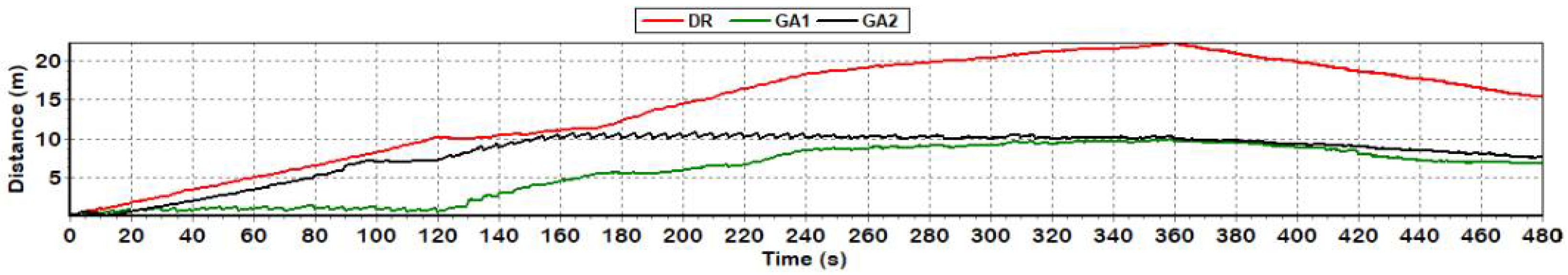
• processing the resulting data into reference drawings with the reference and estimated trajectories of vehicle F, graphs of the distance to the reference position from the estimated position, as well as statistical parameters, i.e., maximum values, arithmetic means, standard deviations of the distance to the reference position from the estimated position.

In terms of the conducted research, many tests have been carried out (assuming various values of measurement parameters), out of which the three most representative were selected, presented below.

3.1. Test No. 1

This test consisted of simulating the movement of vehicle L and vehicle F side by side (relative bearing = 90°) following the same course at the same speed along a path in the shape of a square (i.e., with a simultaneous change of the course by 90° every 120 s). The simulations were carried out assuming the following values concerning the measurement parameters:

• $C^R=45°$ (initial), $f_C=10$ Hz, ${\xi }_C^2=\{\begin{array}{l}4, C^R\in ⟨0,90)\\ 8, C^R\in ⟨90,180)\\ 0, C^R\in ⟨180,270)\\ 2, C^R\in ⟨270,360)\end{array}$;
• $S^R=1m/s$, $f_S=10$ Hz, ${\xi }_S^2=0.05m/s$;
• $D_h^R=10m$, $f_{D_h}=0.2$ Hz, ${\xi }_{D_h}^2=0.025.$

At this point, it should be noted that assuming such significant values of systematic errors ${\xi }_C^2$, ${\xi }_S^2, {\xi }_{D_h}^2$ was intended to simulate the results of measurements performed using navigation devices poorly calibrated for operation in terms of the navigation system on the vehicle.

Figure 3 shows the estimated paths of vehicle F against a background of a reference path obtained as a result of conducting a single (Figure 3a) and a hundred (Figure 3b) test samples as part of test No. 1.

Figure 4 presents graphs of the distance of the reference position from the positions estimated using DR, GA1, and GA2 methods as part of a single test sample (example) in terms of test No. 1.

Table 1. Statistical parameters describing the change of distance to the reference position from positions estimated using the DR, GA1, and GA2 methods.

Positioning Method	Maximum Distance to the Reference Position (m)		Arithmetic Mean of the Distance to the Reference Position (m)		Standard Deviation Distance to Reference Position (m)
	Single Test Sample	100 Test Samples	Single Test Sample	100 Test Samples	Single Test Sample	100 Test Samples
DR	22.31	23.70	14.26	14.13	6.44	6.34
GA1	8.39	8.57	3.42	3.48	2.39	2.41
GA2	15.36	15.36	7.90	7.70	3.68	3.63

presents statistical parameters describing the distance of the reference position from the positions estimated using the DR, GA1, and GA2 methods.

3.2. Test No. 2

This test consisted of simulating the movement of vehicle L and vehicle F one after the other (relative bearing = 180°) following the same course at the same speed along a path in the shape of a square (i.e., a simultaneous change of the course by 90° every 120 s). The simulations were carried out assuming the same values regarding the measurement parameters as in test No. 1.

Figure 5 presents the estimated paths of vehicle F against a background of a reference path obtained as a result of conducting a single (Figure 5a) and a hundred (Figure 5b) test samples as part of test No. 2

Figure 6 presents graphs of the distance of the reference position from the positions estimated using the DR, GA1, and GA2 methods as part of a single test sample (example) in terms of test No. 2.

Table 2. Statistical parameters describing the change of distance to the reference position from positions estimated using the DR, GA1, and GA2 methods.

Positioning Method	Maximum Distance to the Reference Position (m)		Arithmetic Mean of the Distance to the Reference Position (m)		Standard Deviation Distance to Reference Position (m)
	Single Test Sample	100 Test Samples	Single Test Sample	100 Test Samples	Single Test Sample	100 Test Samples
DR	22.31	23.71	14.25	14.13	6.43	6.34
GA1	9.98	10.77	5.78	6.57	3.43	3.81
GA2	10.81	10.89	8.12	8.20	2.99	2.89

presents statistical parameters describing the distance of the reference position from the positions estimated using the DR, GA1, and GA2 methods as part of test No. 2.

3.3. Test No. 3

This test consisted of simulating the movement of vehicle L and vehicle F side by side (relative bearing = 90°) following the same course at the same speed along a path in the shape of a square (i.e., with a simultaneous change of the course by 90° every 120 s). However, the simulations were carried out, in contrast to tests No. 1 and No. 2, assuming very small values of systematic errors:

• ${\xi }_C^2=\{\begin{array}{l}0.4, C^R\in ⟨0,90)\\ 0.8, C^R\in ⟨90,180)\\ 0, C^R\in ⟨180,270)\\ 0.2, C^R\in ⟨270,360)\end{array}$,
• ${\xi }_S^2=0.005m/s$,
• ${\xi }_{D_h}^2=0.0025$,

in order to simulate the results of measurements carried out using navigation equipment correctly calibrated to work in terms of the on-board navigation system.

Figure 7 presents the estimated paths of vehicle F against a background of the reference path obtained as a result of conducting a single (Figure 7a) and a hundred (Figure 7b) test samples as part of test No. 3.

Figure 8 presents graphs of the distance of the reference position from the positions estimated using the DR, GA1, and GA2 methods as part of a single test sample (example) in terms of test No. 3.

Table 3. Statistical parameters describing the change of distance to the reference position from positions estimated using the DR, GA1, and GA2 methods.

Positioning Method	Maximum Distance to the Reference Position (m)		Arithmetic Mean of the Distance to the Reference Position (m)		Standard Deviation Distance to Reference Position (m)
	Single Test Sample	100 Test Samples	Single Test Sample	100 Test Samples	Single Test Sample	100 Test Samples
DR	2.52	3.79	1.56	1.46	0.72	0.78
GA1	0.91	2.55	0.39	0.73	0.21	0.50
GA2	1.6	3.19	0.69	0.77	0.40	0.52

presents statistical parameters describing the distance of the reference position from the positions estimated using the DR, GA1, and GA2 methods in terms of test No. 3.

4. Discussion

When analysing all the results obtained in tests No. 1 and No. 2 carried out assuming poorly calibrated navigation devices (high values of systematic errors ${\xi }_C^2$, ${\xi }_S^2,{\xi }_{D_h}^2$) it can be stated that the GA1 method turned out to be the best in terms of accuracy, and the DR method turned out to be the worst. On the one hand, this may be evidenced by the closest arrangement of paths estimated using the GA1 method in relation to the reference path shown in Figure 3 and Figure 5. This is also confirmed by the graphs in Figure 4 and Figure 6 as well as the statistical parameters in Table 1 and Table 2. It is precisely in the case of vehicle positions estimated using the GA1 method that the most frequent smallest distances from the reference position can be seen on the graphs. The statistical parameters characterizing this distance are also the most favourable for positions estimated using the GA1 method:

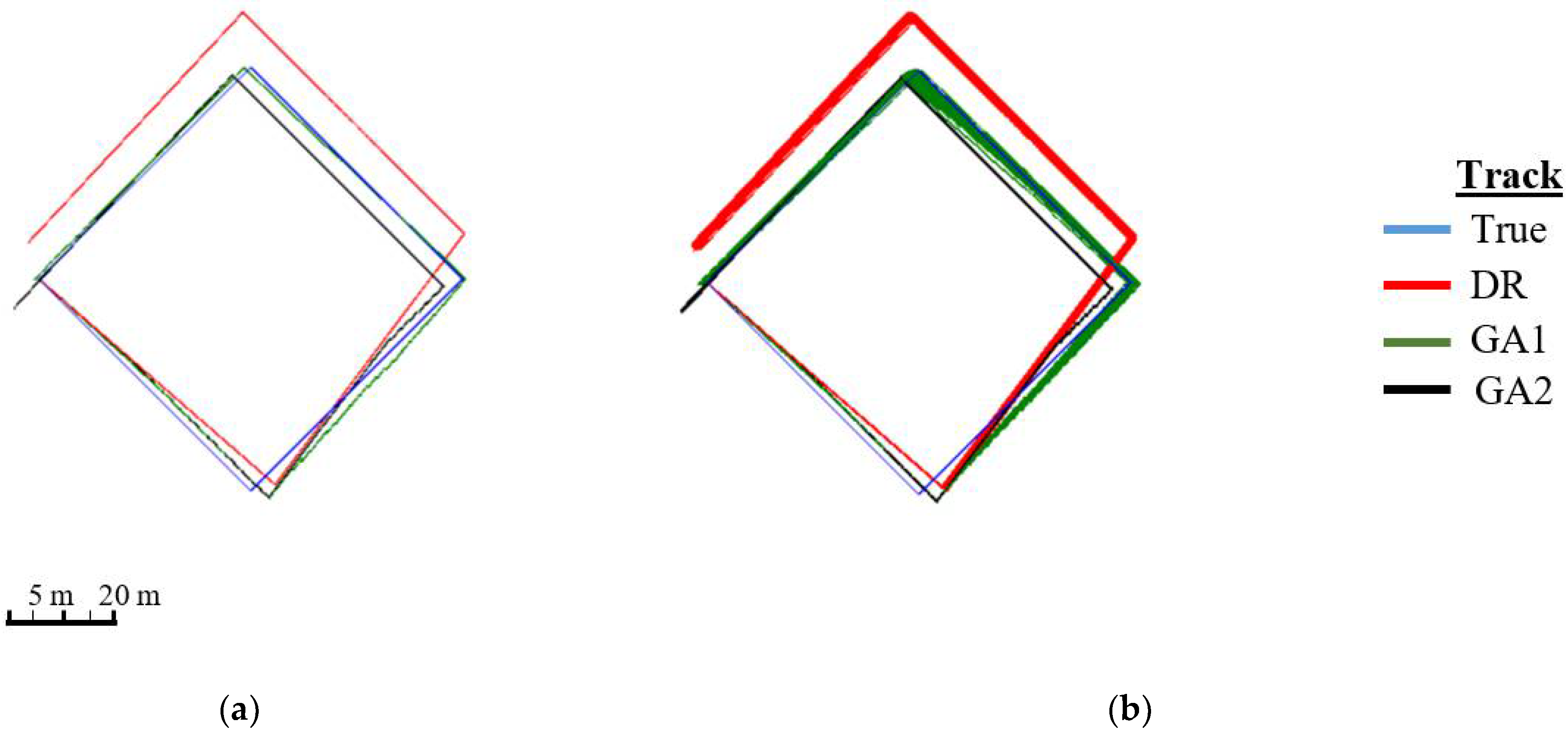
• Test No. 1 (vehicles moving side by side, correct HDOP coefficient) showed that the maximum value, the arithmetic mean, and the standard deviation of the distance to the reference position in the case of positions estimated using the GA1 method are about two times smaller when compared to the distance from positions estimated using the GA2 method, and about three times smaller when compared to the distance from positions estimated using the DR method.
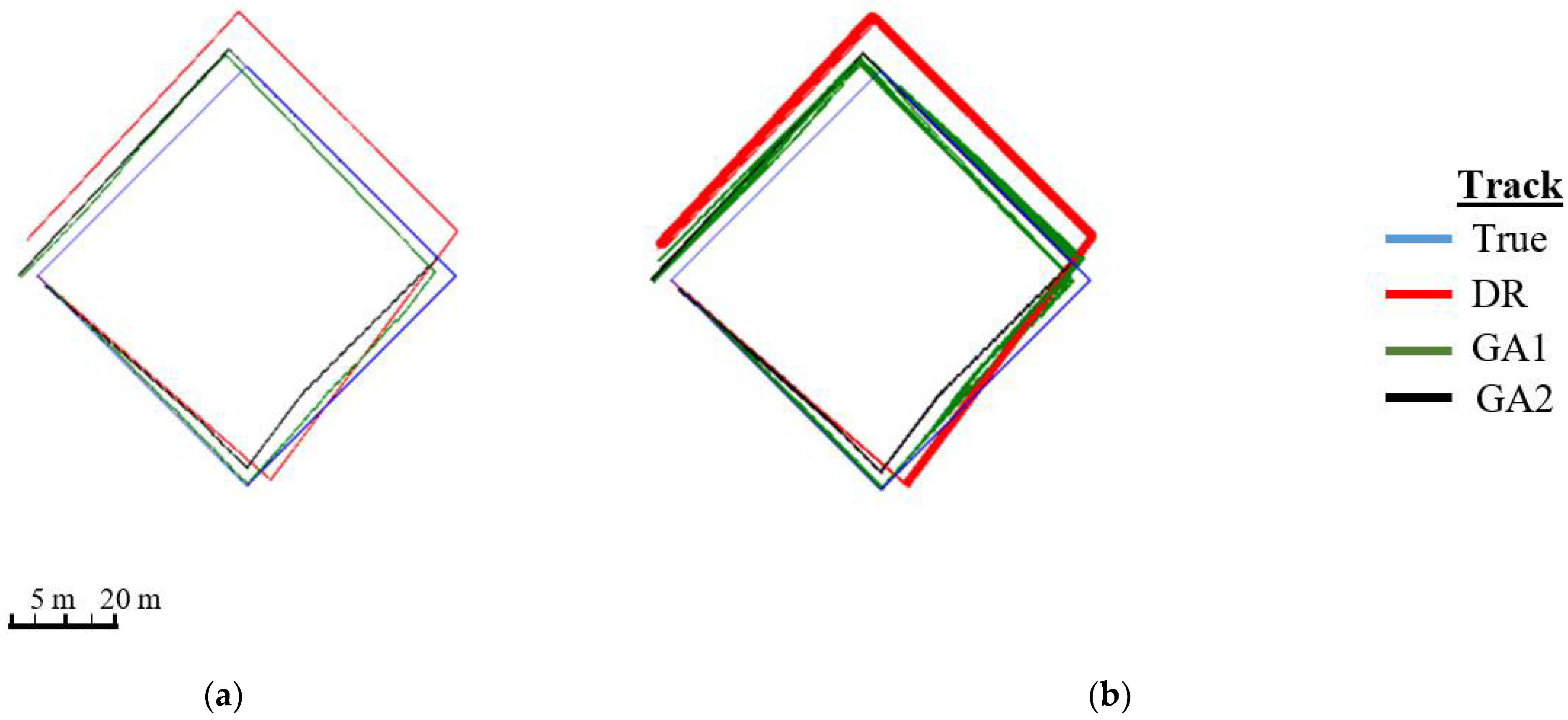
• Test No. 2 (vehicles moving one after the other, incorrect HDOP coefficient) showed that in the case of positions estimated using the GA1 and GA2 methods, the maximum value, the arithmetic mean, and the standard deviation of the distance to the reference position are approximately equal, even though still two times smaller when compared to the distance from the positions estimated with the DR method.

On the other hand, analysing all the results obtained in terms of test No. 3 (vehicles moving next to each other, with a correct HDOP coefficient) carried out with the assumption of properly calibrated navigation devices (small values of systematic errors ${\xi }_C^2$, ${\xi }_S^2, {\xi }_{D_h}^2$), it can be stated that the best and, at the same time, very similar accuracy can be determined for positions estimated using the GA1 and GA2 methods, while positions estimated using the DR method had the worst accuracy.

However, it should be emphasized that the values of statistical parameters of the results of test No. 3 (Table 3) are significantly better compared to the values of statistical parameters of the results of test No. 1 (Table 1). This is illustrated especially by statistical results based on 100 test samples, including the arithmetic mean and the standard deviation of the distance to the reference position from the positions estimated using the GA1 and GA2 methods, equal to approximately:

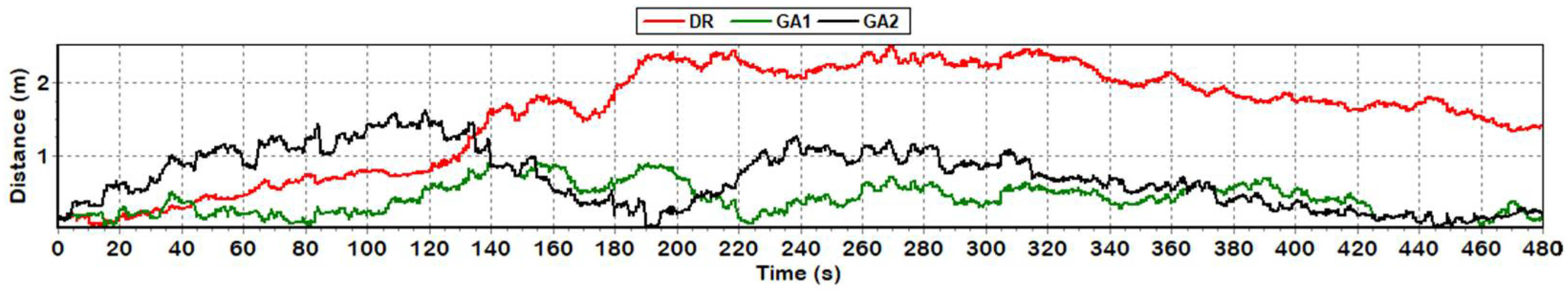
• 0.73 m and 0.5 m for GA1 as well as 0.77 m and 0.52 m for GA2—in the case of test No. 3,
• 3.48 m and 2.41 m for GA1 and 7.7 m and 3.63 m for GA2—in the case of test No. 1.

5. Conclusions

The obtained research results confirmed that it is possible to estimate position coordinates in relation to the leader of the swarm of underwater vehicles with high accuracy, based solely on the results of course and speed measurements, performed with cheap navigation devices, in combination with distance measurement, performed with a hydroacoustic transponder. For this purpose, it is possible to successfully take advantage of the proposed GA1 and GA2 methods (based on geodetic adjustment using the least squares method), taking into account the specificity of their operation. On the basis of the obtained research results, a number of generalized conclusions were drawn in the form of helpful guidelines concerning the optimal use of both methods:

• the GA2 method is most impacted by systematic measurement errors, most often occurring in the case of poorly calibrating navigation devices for working in terms of the on-board navigation system,
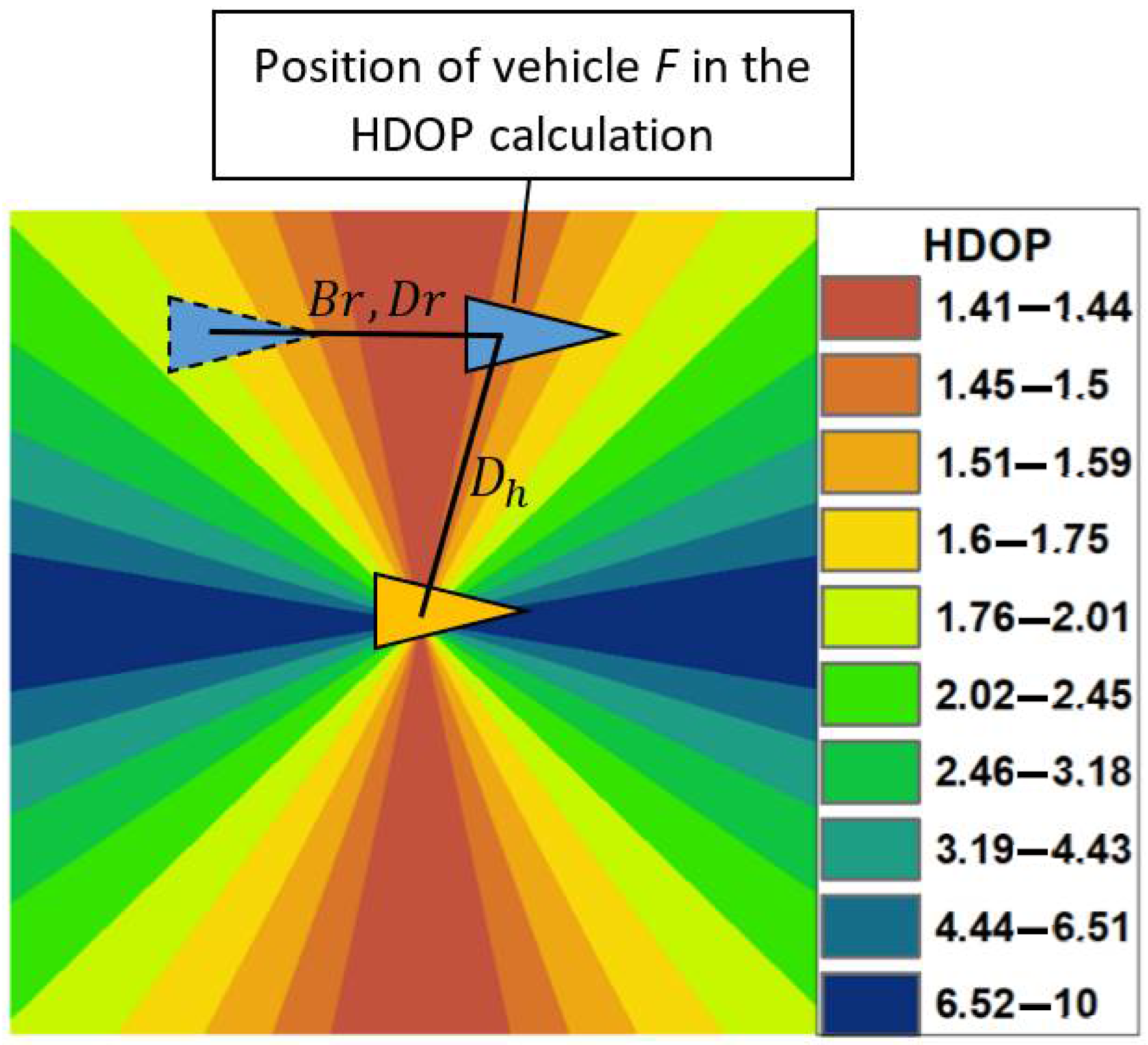
• both methods provide a higher accuracy of estimating position coordinates on abeam angles of the swarm leader (relative bearing equal to approximately ±90°),
• in order to significantly increase the accuracy of estimating position coordinates using both methods, the values of systematic errors of measurements should be minimized (e.g., by calibrating navigation devices to work in terms of the on-board navigation system using a satellite compass and a GNSS RTK receiver),
• the accuracy of estimating coordinates using both methods can also be increased (although to a much lesser extent than in the case of systematic errors) by very accurately and frequently determining the mean error values of the course and speed measurements (e.g., before the start of each task performed by a swarm of vehicles).

Undoubtedly, the main advantages of the proposed methods are:

• estimating position coordinates taking into account course, speed, and distance measurement errors (in the case of the GA 2 method),
• estimating position coordinates taking into account course, speed, and distance measurement errors as well as the geometric shape of the measurement system (in the case of the GA1 method),
• short calculation time and guaranteeing iterative convergence.

However, the main disadvantage concerning the optimal use of the proposed methods consists primarily of the high dependence of the obtained accuracy of estimating position coordinates on the accuracy of estimating the value of course and speed measurement errors. Due to this, further development research relating to both methods should be focused on developing a method of calibrating low-cost navigation equipment measuring the course and speed for working in terms of the described navigation system carried out with the maximum frequency directly on the vehicle.

References

1. Krzysztof, N.; Aleksander, N. The Positioning Accuracy of BAUV Using Fusion of Data from USBL System and Movement Parameters Measurements. Sensors 2016, 16, 1279. [Google Scholar] [CrossRef] [PubMed] [Green Version]
2. Rigby, P.; Pizarro, O.; Williams, S. Towards Geo-Referenced AUV Navigation Through Fusion of USBL and DVL Measurements. In Proceedings of the OCEANS 2006, Boston, MA, USA, 18–21 September 2006; pp. 1–6. [Google Scholar]
3. Lee, P.; Shim, H.; Baek, H.; Kim, B.; Park, J.; Jun, B.; Yoo, S. Navigation System for a Deep-sea ROV Fusing USBL, DVL, and Heading Measurements. J. Ocean Eng. Technol. 2017, 31, 315–323. [Google Scholar] [CrossRef] [Green Version]
4. Barisic, M.; Vasilijevic, A.; Nad, D. Sigma-point Unscented Kalman Filter used for AUV navigation. In Proceedings of the 2012 20th Mediterranean Conference on Control & Automation (MED), Barcelona, Spain, 3–6 July 2012; pp. 1365–1372. [Google Scholar]
5. José, M.; Aníbal, M. Survey on advances on terrain based navigation for autonomous underwater vehicles. Ocean Eng. 2017, 139, 250–264. [Google Scholar]
6. Zhang, T.; Shi, H.; Chen, L.; Li, Y.; Tong, J. AUV Positioning Method Based on Tightly Coupled SINS/LBL for Underwater Acoustic Multipath Propagation. Sensors 2016, 16, 357. [Google Scholar] [CrossRef] [PubMed] [Green Version]
7. Chen, Y.; Zheng, D.; Miller, P.A.; Farrell, J.A. Underwater Inertial Navigation With Long Baseline Transceivers: A Near-Real-Time Approach. IEEE Trans. Control Syst. Technol. 2016, 24, 240–251. [Google Scholar] [CrossRef]
8. Lee, P.-M.; Jun, B.-H. Pseudo long base line navigation algorithm for underwater vehicles with inertial sensors and two acoustic range measurements. Ocean Eng. 2007, 34, 416–425. [Google Scholar] [CrossRef]
9. Jianhua, B.; Daoliang, L.; Xi, Q.; Rauschenbach, T. Integrated navigation for autonomous underwater vehicles in aquaculture: A review. Inf. Process. Agric. 2020, 7, 139–151. [Google Scholar]
10. Karimi, M.; Bozorg, M.; Khayatian, A.R. A comparison of DVL/INS fusion by UKF and EKF to localize an autonomous underwater vehicle. In Proceedings of the 2013 First RSI/ISM International Conference on Robotics and Mechatronics (ICRoM), Tehran, Iran, 13–15 February 2013; pp. 62–67. [Google Scholar]
11. Dajun, S.; Cuie, Z.; Miao, Y.; Yixian, S. Research and Implementation on Multi-beacon Aided AUV Integrated Navigation Algorithm Based on UKF. In Proceedings of the 2nd International Conference on Vision, Image and Signal Processing (ICVISP 2018), Association for Computing Machinery, New York, NY, USA, 27 August 2018; pp. 1–5. [Google Scholar] [CrossRef]
12. Almeida, J.; Matias, B.; Ferreira, A.; Almeida, C.; Martins, A.; Silva, E. Underwater Localization System Combining iUSBL with Dynamic SBL in ¡VAMOS! Trials. Sensors 2020, 20, 4710. [Google Scholar] [CrossRef] [PubMed]
13. Miller, A.; Miller, B.; Miller, G. Navigation of Underwater Drones and Integration of Acoustic Sensing with Onboard Inertial Navigation System. Drones 2021, 5, 83. [Google Scholar] [CrossRef]
14. González-García, J.; Gómez-Espinosa, A.; Cuan-Urquizo, E.; García-Valdovinos, L.G.; Salgado-Jiménez, T.; Cabello, J.A.E. Autonomous Underwater Vehicles: Localization, Navigation, and Communication for Collaborative Missions. Appl. Sci. 2020, 10, 1256. [Google Scholar] [CrossRef]
15. Normal_Distribution Class Template. Available online: https://cplusplus.com/reference/random/normal_distribution/ (accessed on 29 September 2022).
16. IMU VN-100 User Manual. Available online: https://www.vectornav.com/products/detail/vn-100 (accessed on 29 September 2022).
17. Electromagnetic Speed Log Alize. Available online: https://cdn.echomastermarine.co.uk/assets/Uploads/Ben-Marine-ALIZE-EM-Log.pdf (accessed on 20 September 2022).
18. HS Underwater Acoustic Modems. Available online: https://evologics.de/acoustic-modem/hs (accessed on 23 September 2022).
19. C++Builder. Available online: https://www.embarcadero.com/products/cbuilder (accessed on 25 September 2022).
20. Eigen is a C++ Template Library for Linear Algebra. Available online: https://eigen.tuxfamily.org/index.php?title=Main_Page (accessed on 20 September 2022).
Figure 1. Idea diagram of the navigation measurement system in the leader–single swarm vehicle relation.
Energies 15 08472 g001
Figure 2. Distribution of the HDOP coefficient in the swarm leader–single vehicle relation (a proprietary app has been prepared with the use of the inverse distance weighting interpolation method).
Energies 15 08472 g002
Figure 3. Reference and DR, GA1, GA2 estimated paths of vehicle F obtained in the course of conducting: (a) A single test sample; (b) A hundred test samples.
Energies 15 08472 g003
Figure 4. Distance to reference position from positions estimated using DR, GA1, GA2 methods as a function of time (single test sample).
Energies 15 08472 g004
Figure 5. Reference and DR, GA1, GA2 estimated paths of vehicle F obtained in the course of conducting: (a) single test sample; (b) hundred test samples.
Energies 15 08472 g005
Figure 6. Distance to reference position from positions estimated using DR, GA1, GA2 methods as a function of time (single test sample).
Energies 15 08472 g006
Figure 7. Reference and DR, GA1, GA2 estimated paths of vehicle F obtained in the course of conducting: (a) single test sample; (b) hundred test samples.
Energies 15 08472 g007
Figure 8. Distance to reference position from positions estimated using DR, GA1, GA2 methods as a function of time (single test sample).
Energies 15 08472 g008