Abstract
A recloser requires a fast operating time in the first shot to optimally clear a temporary fault. The operating time is dependent on the time-dial, the pick-up settings, and the fault current. The recloser detects the fault current from the grid supply; however, the connection of the generators in the distribution system can contribute to the fault current. Depending on the location of the generators and the direction of the current, the fault current can decrease and cause an increase in the operating time. Therefore, the optimal settings that can minimize the operating time may need to be determined. This paper simulates the behavior of a recloser in its first shot for clearing a temporary fault and tests its performance in an active distribution system that has two types of distributed generators. It then uses the differential evolution algorithm to find the optimal settings in the active distribution voltage conditions. It also applies modifications to the differential evolution algorithm and uses these modifications to find robust settings. It then uses an exponential scale factor to balance the exploration and exploitation of the algorithm chosen. Simscape power systems in Matlab Simulink is used to construct the active distribution system and simulate the cases, while the Matlab script is used to run the code for the differential evolution algorithm. Six cases are performed to find the optimal settings of the recloser. The results show that the selected settings and the differential evolution algorithm modification can optimize the operation of the recloser.
1. Introduction
Distribution systems are traditionally radial and passive. The settings of reclosers are based on the assumption of the grid supply, and the recloser clears a temporary fault optimally as set [1]. However, the recent advancements in improving the voltage profile and deregulating the grid through the connection of distributed generation required a reassessment of the settings of the recloser and its optimal operation. This is because there is another fault current contributor when the distributed generation operates in a grid-connected mode [2]. A prevailing practice was to isolate the distributed generators during a fault; however, a substantial rise in distributed generation penetration has led to a standard requiring distributed generation to remain grid-connected during a fault. The connection of distributed generators introduces a new fault current and a different direction of the fault current compared to the conventional downstream direction in the fault current detected by the recloser. The recloser can have a varied operating time because of the varied magnitude and change in direction of the fault current. The varied operating time is caused by the inverse time-current characteristic of the recloser. The varied operating time can lead to a shorter response or longer response of the recloser compared to the operating time that it was set to have in the passive distribution system [3,4].
In the case of a recloser having a longer operating time, a population-based algorithm or metaheuristic optimization algorithm can be used in searching for optimal settings and reducing the operating time [5]. These settings can improve the operation of the recloser when distributed generators are grid-connected during a temporary fault. Population-based algorithms provide a method of obtaining optimal solutions through the formulation of linear or non-linear optimization problems and through iterative steps. Research has shown that the differential evolution algorithm is one of the best-performing population-based algorithms for solving an optimization problem. The advantage of using this technique is that it performs a stochastic search through the feasible region of solutions, it is capable of handling non-linear and non-differentiable functions, and it can easily escape from a local optimum [6].
Therefore, to enable a fast reconnection during a temporary fault, appropriate settings need to be set for the recloser. This is to optimize the operation of the recloser when the distributed generators are grid-connected [7,8]. With this regard, the paper explores the feasibility of designing and using a differential evolution algorithm scheme with a balanced exploration and exploitation scale factor. This scheme is for searching and selecting the global optimal settings of the recloser in a distribution system connected with distributed generation. The variation in the voltage profile is assessed, and the selection of the optimal settings is automated. This paper modifies the differential evolution algorithm to obtain the best-performing scheme under the system’s conditions and solves the exploration and exploitation of the selected algorithms. After the introduction, the study is organized as follows: Section 2 presents a literature review, Section 3 presents materials and methods, Section 4 presents the results, Section 5 presents the discussion, and conclusions are drawn in Section 6.
2. Literature Review
Distributed generators were initially configured to adhere to the IEEE 1547 grid code requirement during temporary faults or temporary disturbances. They were to be disconnected from the grid quickly during these disturbances. However, according to [9], with the increasing penetration of distributed generation, grid codes are changed in some high and extra-high voltage grid connection standards (i.e., 1 kV to 60 kV) to have them remain grid-connected during these disturbances. This makes the penetration level very important in fault conditions. The distributed generation penetration level in the distribution system can be determined by using (1).
where PDG and PLoad are the power from the distributed generation and the power consumed by the loads.
The modes that can result in the voltage profile of the distribution system caused by the penetration of distributed generation are given below [5]:
- Flat voltage profile: the penetration level is equal to 100%, (i.e., the power consumed equals the power of the distributed generation, and the voltage profile is the same for the entire distribution system).
- Rising voltage profile: the penetration level exceeds 100%. More power penetrates the upstream system and causes a rising voltage to the distribution system toward the end of the feeder.
- Falling voltage profile: The penetration level is below 100%. The voltage decreases toward the end of the feeder in the distribution system.
In [10], the relationship between the voltage profile and the fault conditions is investigated. Faults are initiated in the different nodes of an active distribution system, and it is determined that the distributed generation added a 2% voltage improvement at any severely affected node. In [11], it is stated that the contribution of synchronous-based distributed generators to the fault current level ranges from five to six times its rated current and the contribution of the inverter-based distributed generation to the fault current level ranges from 1.1 to 2 times its rated current.
2.1. Recloser Operation Time
In the setting of reclosers to act on a suitable curve for an optimal fast operating time, suitable settings must be designed for the recloser to have successful operations and limit the effects of mal-operations such as protection blinding and the recloser losing coordination with the fuse. In [12], the operating time of the recloser is expressed as an inverse function of the fault current flowing through it. The recloser operates with an IEC/IEEEE very inverse curve in the fast mode and an IEC/IEEE extremely inverse curve in the delayed mode. A time-current curve has three main operating regions; the overload region, the adjustable instantaneous region, and the instantaneous region. The last two regions are needed to clear faults while the overload region protects the system in cases of emergencies. An optimal fast operating time of the recloser should be between 100 milliseconds to 200 milliseconds within the instantaneous and adjustable instantaneous region [13]. The variation of the operating time is subject to the type, location, and penetration of the distributed generators. A double-fed induction generator wind turbine generates a high sub-transient fault current but gradually drops after the first cycle, requiring a fast operation time of the recloser for temporary faults within the first cycle [14].
2.2. Differential Evolution Algorithm
Optimal settings can be obtained by solving the recloser’s increase in operating time as an optimization problem. Particle swarm optimization, ant colony, and differential evolution algorithms can be applied to obtain Pareto solutions for these settings [15,16]. The selection of a robust algorithm is dependent on the convergence and global optimal solution search. Among these three algorithms, the particle swarm optimization only continues the search with the same particles and no other particles are substituted during iterations, which can limit the global search for the optimal solution [17]. The ant colony optimization’s convergence speed is low, and this algorithm performs better for a local search than for a global search [15,18]. The differential evolution is an algorithm that was proposed by Kenneth V. Price and R. Storn in 1997 to solve optimization problems [19]. It is a child of the genetic algorithm by the addition of the differential mutation operator. The differential evolution algorithm was proposed for minimizing non-linear functions; it is a simple and efficient meta-heuristic algorithm in solving for global optimal solutions. The algorithm continues the search with the best vectors through mutation and selection operations for the computation of an optimal solution. Joymala Moirangthem et al. [11] apply it to search for the global optimum relay coordination settings in a distributed generation system. A design of the differential evolution algorithm scheme can be applied with a balanced exploration and exploitation scale factor to quickly compute global optimum settings and improve robustness and convergence.
Different authors have highlighted the use of the differential evolution algorithm, stating its advantages and disadvantages. They have also tested the performance against other optimization algorithms to show the robustness and computational efficiency of the differential evolution algorithm. In [19], a relay coordination problem is formulated to obtain the minimum possible operating time for optimal coordination. The fitness function is the summation of operating times of the primary overcurrent relays. The optimization problem is solved using the differential evolution algorithm, and the optimal relay settings are obtained with a standard inverse time-current characteristic model. The time-dial and pick-up settings are optimized for this model. The overcurrent relays had a long operating time when there was the solar photovoltaic system connection, but they were optimized with the model used to obtain optimal settings. In [20], the coordination of the inverse definite minimum time overcurrent relays is formulated as a constrained optimization problem, the objective is to minimize the total operating time of all the directional overcurrent relays. The optimization problem has twelve decision variables in the first case and twenty-eight decision variables in the second case; the optimal settings are obtained by the differential evolution algorithm. The differential evolution algorithm converges before the iterations are completed, and this can limit it from determining the best global solution; because of this, it can be modified. In [21], the differential evolution algorithm is consistently ranked as one of the best search algorithms for solving global optimization problems. A mutation to the differential evolution algorithm is presented for five modified schemes; the modification is made on the weighted difference, and the scaling factor is varied following the Laplace distribution. The differential evolution variant can be denoted as DE/X/Y/Z, where X is the vector mutated, Y is the number of the difference vectors used, and Z is the crossover of the scheme. One of the performance metrics considered to determine the scheme that is robust and efficient is the fitness function value. In [22], the differential evolution algorithm is compared to the genetic algorithm in terms of accuracy, robustness, and computational efficiency for the design of a radial flux permanent magnet generator. The differential evolution algorithm had a higher fitness value and a lower standard deviation from a stochastic point of view, meaning it performed better than the genetic algorithm; it also had a better convergence rate when the population was decreased.
2.3. Exponential Scale Factor
The differential mutation step is varied by applying a varied scale factor. This is to guarantee that the search for the best-performing decision variables is maximized. The exploration and exploitation of the differential evolution algorithm needs to be balanced. The differential evolution algorithm has to be able to explore the global time-dial and pick-up settings while having an optimal ability to refine the identified search area and find the optimal settings. To ensure a balanced exploration and exploitation ability, the scale factor is modified according to (2). High values of the scale factor will enhance the exploration of the search area; as the scale factor decreases exponentially, the exploitation will be enhanced [23].
where Itmax is the maximum number of iterations and It is the current iteration.
3. Materials and Methods
The settings should minimize the operating time compared to the conventional settings. The time-dial and pick-up decision variables are subject to design constraints that limit the search within their minimum and maximum parameter setting.
3.1. Problem Formulation
The change in the operating time of the recloser is a non-linear optimization problem since the recloser’s operation time is determined from a non-linear function expressed in (3). Only the TD and IP are unknown independent decision variables. A, B, p, and IR are known.
where i is the recloser identifier, TR is the operating time of the recloser; TD is the time-dial setting, IR is the current detected by the recloser, IP is the pick-up setting, and A, B, and p are the constants for a particular time-current characteristic curve.
The objective is to minimize the operating time of the fast curve. The form of the objective function is expressed in (4)
OF = Min TRi
3.2. Recloser Settings Constraints
The range of the recloser settings from which feasible solutions are selected is presented as constraints in (5) and (6); these are the constraints of the time-dial and pick-up settings of the recloser.
where TDmin is the minimum limit of the time dial settings, TDmax is the maximum limit of the time dial setting, IPmin is the minimum limit of the pick-up setting, and IPmax is the maximum limit of the pickup setting.
3.3. Differential Evolution Algorithm Pseudo-Code
The algorithm used is the DE/rand/1/bin. The inputs of the differential evolution algorithm are the fitness function (), lower bound (, upper bound ( of the decision variables, population size (), number of generations (), scaling factor (), and cross-over the property () [21,24,25].
Step 1: Initializing the differential evolution parameters (random).
The target vectors in (7) are initialized randomly in (8) to create a random population. This is the random selection of the initial population for optimal solutions of the decision variables. These values are selected between their minimum and maximum limits.
where, g = 1, 2, ……., G is the maximum number of generations, = 1, 2, ……., D is the problem dimension, and is the uniformly distributed random variable within the range of (0, 1).
Step 2: Differential mutation (one differential operator)
For g = 1 to G do Loop for generation.
For k = 1 to P do Loop for the population size.
The mutated vectors of the time dial and pick-up decision variables are generated by using (9).
where, r1, r2 and r3 ϵ {1, 2.…. P} are random integers, different from each other and the running index [24,25].
The mutated decision variables are presented in (10).
Step 3: Crossover
In the crossover, a trial vector is generated using an if statement. A trial vector is selected by (11).
end → end loop for the population size.
Step 4: Selection (binomial)
For i = 1 to D do
To generate a new population with optimal solutions, the differential evolution algorithm replaces the target vector with the trial vector using (12).
end → end loop for selection.
end → end loop for generation.
3.4. Differential Evolution Algorithm Modified Schemes
The recloser should trip within 100 to 200 msec from the start of the fault and reclose after the dead time. It should operate optimally to extinguish the fault, prohibiting the operation of downstream protection devices. The differential evolution algorithm can be modified to design three schemes that should each individually enhance the performance of the recloser and meet these requirements. This is to find the optimal settings for the different voltage profiles. The schemes use the weighted difference between the two points. The mutation strategies and modifications are presented in Table 1.

Table 1.
Differential Evolution Algorithm Modified Schemes.
3.5. Methodology
To select and test the optimal settings for different voltage profiles. The IEEE 34-node distribution feeder is adopted as a passive distribution system with an existing load flow and system conditions. The feeder is supplying voltage to three-phase, two-phase, and single-phase loads. This system operates with a 12 MVA, 60 Hz, 60/24.9 kV step-down transformer in the sub-station. The components of the system are protected by recloser R for selecting temporary faults. The single-line diagram of the distribution system is depicted in Figure 1. The nodes where the distributed generators are connected and the three-phase fault are shown. The rest of the nodes can be observed in the reference provided. The data for the feeder can be found in the IEEE Distribution Analysis Subcommittee article. The wind turbine and solar photovoltaic systems are integrated as a phase-to-phase in the ungrounded three-phase section of the feeder. The energy storage system is integrated as a single phase into the second phase of the distribution. These active distribution system conditions are simulated in MATLAB Simulink [18,19].
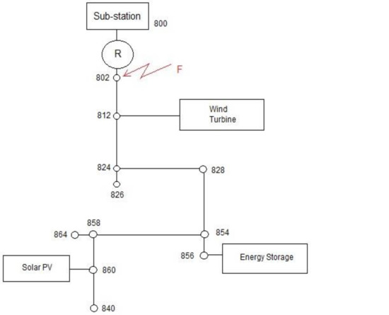
Figure 1.
Application of a recloser in a radial distribution feeder with distributed generation integrated [26,27].
The distributed generators connected to the distribution system depicted in Figure 1 cause the voltage profile to vary depending on the type of distributed generation. The investigation shall be conducted for the three types of voltage profiles that are caused by the connection of these distributed generators. The cases are simulated to observe the performance of the recloser when the recloser uses conventional settings or the differential evolution algorithm selected settings for the voltage profiles shown in Figure 2. Each voltage profile in Figure 2 represents a flat voltage profile, rising voltage profile, or falling voltage profile, which form the bases of the cases studied for determining a scheme that is best for optimizing the recloser setting and applying it for obtaining the settings. The voltage profiles show a variance between 0.6 p.u. to 0.8 p.u along the distribution feeder.
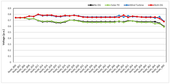
Figure 2.
Active Distribution system voltage profiles.
4. Results
To facilitate an optimal recloser operation, the recloser should trip and reclose before the temporary fault can cause damage; it should operate to extinguish the fault prohibiting the operation of the downstream protection devices. The recloser should act selectively to clear the temporary fault on the first shot. The new line current and fault current detected by the recloser in the presence of distributed generation are used to obtain the optimal time-dial and pick-up settings. The differential evolution algorithm in Section 3 is implemented in MATLAB; the results of the algorithm for each scheme are given in Table 2. To adjust the operating time and the pick-up of the recloser, a time-dial setting can be adjusted by a step size of 0.05 s and the pick-up can be adjusted by a step size of 25%. The curves obtained through the conventional settings and differential evolution algorithm-selected settings can be shown in Figure 3. As can be seen, the differential evolution algorithm provides better settings which can improve the operating time. The differential evolution algorithm is further modified into schemes. The schemes should provide an improved differential evolution algorithm to meet the objective function. The fault is at node 802, and the conventional settings and optimal settings are presented in Table 2. The control signals of the recloser using conventional settings and the settings obtained through the differential evolution algorithm are shown in Figure 4 and Figure 5. These show the peak of the fault current and the responses of the recloser when the fault is temporary or permanent. The figures show when the fault was initiated, the duration, and when it ceased. The duration for the temporary fault is 0.1 s. The results show that the recloser can be optimized for both temporary and permanent faults, but the recloser is mainly needed to be optimized for a temporary fault and improve its speed, selection, and sensitivity to clear temporary faults before they can cause mal-operations in the protection scheme.
Table 2.
Time Dial and Pickup settings for Conventional, DE and MDE schemes.
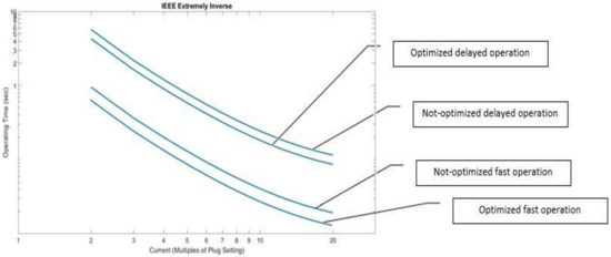
Figure 3.
Comparison of the fast and delayed curves for the recloser using conventional settings and differential evolution algorithm settings.
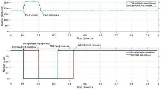
Figure 4.
Comparison of the non-optimized and optimized operations for the recloser during a temporary fault.
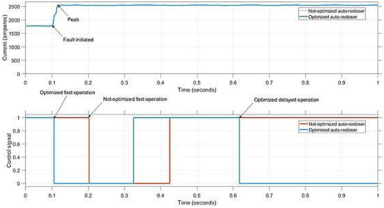
Figure 5.
Comparison of the non-optimized and optimized operations for the recloser during a permanent fault.
The line current and fault current passing between node 800 to node 802 is altered when there is a connection of distributed generation. When there is a solar photovoltaic system, the current is almost the same as when there is no distributed generator connected, but when there is a wind turbine connected, the fault increases the current from 0.02 p.u. to 0.08 p.u. When both the distributed generators are connected, the current increases from 0.02 p.u. to 0.07 p.u.
4.1. Case 1 Temporary Fault Clearance for No Distributed Generation Voltage Profile
The recloser response to the fault for the voltage profile when there is no distributed generator connected is simulated in this case study. The performances of the conventional and optimal protection settings of the recloser are simulated. Figure 6 depicts the response of the recloser when the fault strikes node 802. It can be observed that the magnitude of the current rises to 2370 A at 0.1 s. The fault is temporary and lasts for 0.2 s. It begins at 0.1 s and ends at 0.3 s. The recloser’s conventional settings operate the recloser in a time of 0.1318 s after the fault is initiated. The DE settings have an operation time of 0.1970 s, the MDE settings give an operation time of 0.0340 s, the MDE1 settings give an operation time of 0.0540 s, and the MDE2 settings give an operation time of 0.0820 s. As depicted in Figure 6, the two sets of settings that optimize the performance of the recloser are MDE1 and MDE3 for a fast trip command. The settings impact on the dead-time before the reclosure of the circuit breaker. The recloser has a successful reclosing after the temporary fault has self-cleared [27].
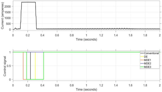
Figure 6.
Fault clearance with conventional and optimum settings for no distributed generation voltage profile.
4.2. Case 2 Temporary Fault Clearance for a Falling Voltage Profile Mode in F1
The operation of the recloser in the falling voltage profile mode is simulated in this case study. This falling voltage profile mode is caused by the penetration level of the solar photovoltaic system. Figure 7 depicts the response of the recloser. The performances of the conventional and optimal protection settings are simulated. The fault is temporary with a duration of 0.2 s. The fault current level rises to 2370 A at 0.1 s. The time taken to send the trip signal from the recloser’s control circuit using the conventional settings is 0.1318 s. When the settings are changed from conventional to DE, the time is 0.1977 s. When the settings are changed from conventional to MDE1, the time is 0.0342 s. When the settings are changed from conventional to MDE2, the time is 0.5464 s, and when the settings are changed from conventional to MDE3, the time is 0.0850 s. In this case, MDE 1 and MDE3 show an optimal performance for the recloser. They can isolate the fault faster than the conventional settings. However, the dead time of the recloser seems to vary.
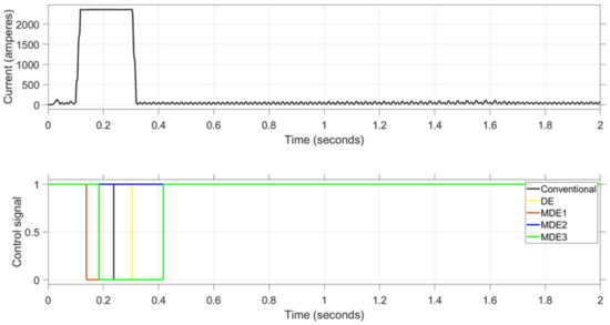
Figure 7.
Fault clearance with conventional and optimized settings for a falling voltage profile mode.
4.3. Case 3 Temporary Fault Clearance for a Rising Voltage Profile Mode in F1
The recloser operates in a rising voltage profile of the distribution system. The rising voltage profile is caused by the penetration of the wind turbine system. Figure 8 depicts the response of the recloser. It can be observed that the fault strikes at 0.1 s. It is a temporary fault and has a duration of 0.2 s. The distributed generator is assumed to have a low voltage ride-through during the temporary fault. The magnitude of the current rises to 2358 A due to the fault. The recloser sends a trip signal to the circuit breaker after a fast operating time dictated by the settings. The operating time of the recloser for the conventional settings is 0.1800 s, for the DE, it is 0.1959, for the MDE1, it is 0.0331 s, for the MDE2, it is 0.5437 s, and for the MDE3, it is −0.0640 s. MDE3 shows increased sensitivity to transient fluctuations in the line current. It responds before the fault begins. The optimal settings, in this case, are provided by MDE1. MDE3 also provides the optimal settings, but it is sensitive to the changes in the current. It can be observed that the dead time varies in response to changes in the settings.
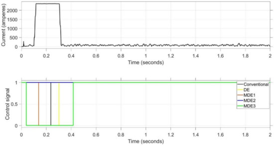
Figure 8.
Fault clearance with conventional and optimum settings for a rising voltage profile.
4.4. Exponential Scale Factor Application for Case 1
The two best-performing schemes that have been identified are MDE1 and MDE3. For the MDE1 the new time-dial and pick-up settings using the exponential scale factor are 0.05 and 175, and for MDE3, the new time dial and pick-up settings are 0.15 and 100. Figure 9 depicts the response of the recloser when the settings applied are obtained through a scale factor varied exponentially. The magnitude of the current rises to 2370 A at 0.1 s; this is caused by the fault. The fault is temporary, with a duration of 0.2 s. The exponential scale factor application produced a fast operating time of 0.0847 s using the MDE1 settings and a fast operating time of 0.0856 s using the MDE3 settings. The recloser sends trip commands to the circuit breaker after these time delays. It can be observed that the dead-time does not vary. The auto-recloser recloses the circuit breaker after the dead-time.
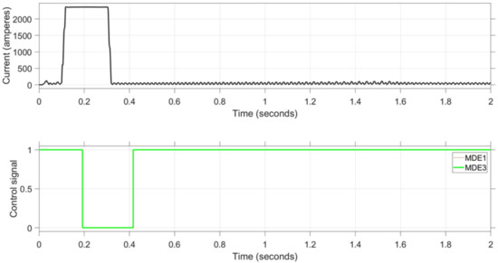
Figure 9.
Recloser response for MDE1 and MDE3 in case 1.
4.5. Case 5 Exponential Scale Factor Application for Case 2
Figure 10 depicts the response of the recloser when the settings applied are obtained from MDE1 and MDE3 with an exponentially varied scale factor. The fault occurs at 0.1 s with a duration of 0.2 s. The current rises to a magnitude of 2370 A when the fault begins. The fast-operating time of the recloser is 0.0800 s when the settings of MDE1 are used. When the settings of MDE 3 are used, the recloser operates with a fast operating time of 0.1024 s. The dead time is fixed on 0.2 s with a slight variation in MDE1.
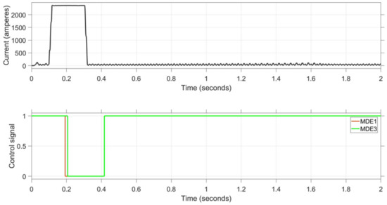
Figure 10.
Recloser response for MDE1 and MDE3 in case 2.
4.6. Case 6 Exponential Scale Factor Application for Case 3
Figure 11 depicts the response of the recloser for the settings obtained using MDE1 and MDE3 when the scale factor is exponentially varied. The fault begins at 0.1 s, and the current level rises to 2370 A. The fault is temporary and has a duration of 0.2 s. The time that the recloser responds with is 0.0847 s when using the settings obtained by the MDE1 algorithm. The operating time of the recloser is 0.1091 s using the MDE3 algorithm. MDE1 performs better than MDE3, giving a set of optimal settings that can be used to minimize the recloser operating time.
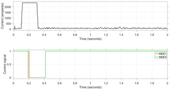
Figure 11.
Response for MDE1 and MDE3 in Case 3.
5. Discussion
Three case studies with different voltage profiles of the distribution system have been simulated. The voltage profiles are a result of the integration of the distributed generation. The case studies optimize and analyze the clearance of a temporary fault by the recloser using five different sets of time-dial and pick-up settings. These five sets of settings are from the conventional method, differential evolution algorithm, and modified differential evolution algorithms. In each case, node 802 of the distribution system presented in Figure 1 had a fault initiated. The fault is a three-phase-to-ground, and the response of the current was taken from a single phase to observe what the current level rises to. The three-phase-to-ground represents the worst-case scenario. The control circuit signal was also observed.
Figure 12 presents the comparison of the recloser operating times when simulated with the conventional settings and settings obtained from differential evolution algorithm schemes. The response of the recloser is determined during the sub-transient state of the fault current. DE and MDE2 schemes computed a set of results that showed a delayed response; this can be due to the premature convergence of the schemes. The conventional, MDE1, and MDE3 schemes showed a faster response, not surpassing the optimal 0.2 s fast-operating time. This keeps the recloser fault clearance within the instantaneous and adjustable instantaneous operating region. The connection of the solar photovoltaic system and wind turbine systems showed variations in the operating times. MDE3 became sensitive to the intermittency introduced by the wind turbine system and operated before the fault started. This needed a better selection of settings from this scheme.
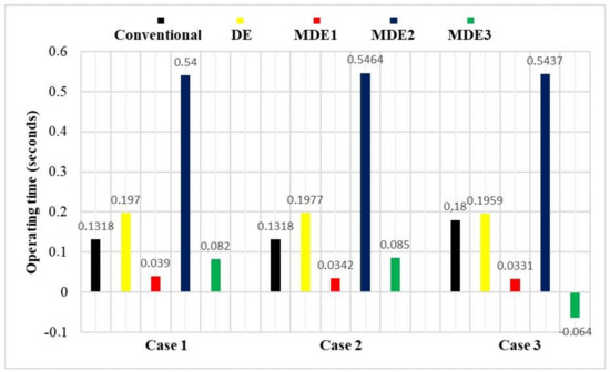
Figure 12.
Recloser operating time for the different settings.
MDE1 and MDE3 are compared with each other in Figure 13. The application of an exponential scale factor was to obtain the most optimal settings and operation of the recloser for this active distribution system between MDE1 and MDE3. In case 1, case 2, and case 3, the MDE1 computes a lower operating time of the recloser than the MDE3. MDE3 shows an increasing operating time as the type of distributed generation system and voltage profile of the distribution system changes. The MDE1 settings prove to be superior and enhance the response of the recloser.
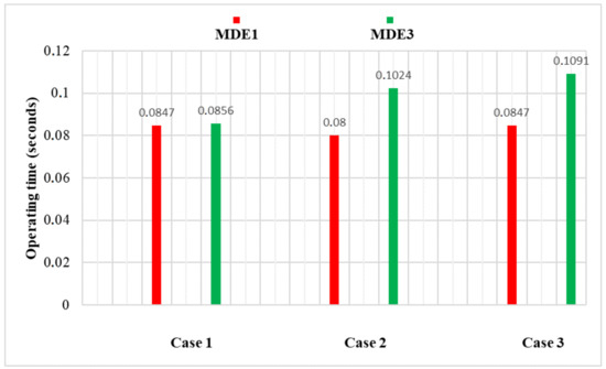
Figure 13.
MDE1 and MDE3 settings’ performance with an exponentially varied scale factor.
6. Conclusions
The three-voltage profiles that can result from the integration of distributed generation formed a foundation to test and analyze the operation of the recloser. The connection of the different types of distributed generation systems into the IEEE 34 node distribution system presented voltage and current level conditions that required a design of settings to produce an optimal operating time for a temporary fault. The recloser was applied in this distribution system for automated responses in protecting it against temporary faults. The requirement for optimal protection from the recloser is that the fast operating time should not surpass the range of 0.1 s to 0.2 s. This is to keep it from having issues such as protection blinding and mis-coordination with other protection devices. Five settings were tested and analyzed in three case studies. Two of the settings from the differential evolution algorithms showed superior performance when compared to the other three settings.
The two modified schemes of the differential evolution algorithm demonstrated the capability to search and select optimal settings that can optimize the operation of the recloser when there is a connection of distributed generation. They maintained an optimal performance when the distribution system was connected with the solar photovoltaic system however some sensitivity issues needed to be mitigated when there was an integration of the wind turbine system. Varying the scale factor of the two schemes aimed to refine the search area and balance the exploration and exploitation of the modified schemes. This was tested under the three cases and MDE1 proved to compute better-performing settings than MDE3.
Author Contributions
Conceptualization, S.B.G. and A.K.S.; methodology, S.B.G. and A.K.S.; software, S.B.G.; validation, S.B.G. and A.K.S.; formal analysis, S.B.G. and A.K.S.; investigation, S.B.G.; resources, S.B.G. and A.K.S.; data curation, S.B.G.; writing—original draft preparation, S.B.G.; writing—review and editing, A.K.S.; visualization, S.B.G. and A.K.S.; supervision, A.K.S.; project administration, A.K.S. All authors have read and agreed to the published version of the manuscript.
Funding
This research received no external funding.
Data Availability Statement
Not applicable.
Conflicts of Interest
The authors declare no conflict of interest.
References
- Lilla, A.D.; Khan, M.A.; Barendse, P. Comparison of Differential Evolution and Genetic Algorithm in the design of permanent magnet Generators. In Proceedings of the 2013 IEEE International Conference on Industrial Technology (ICIT), Cape Town, South Africa, 25–28 February 2013; pp. 266–271. [Google Scholar] [CrossRef]
- Atteya, A.I.; El Zonkoly, A.M.; Ashour, H.A. Optimal Relay Coordination of an Adaptive Protection Scheme using Modified PSO Algorithm. In Proceedings of the 2017 Nineteenth International Middle East Power Systems Conference (MEPCON), Cairo, Egypt, 19–21 December 2017; pp. 689–694. [Google Scholar] [CrossRef]
- Chandra, A.; Singh, G.K.; Pant, V. Protection of AC microgrid integrated with renewable energy sources—A research review and future trends. Electr. Power Syst. Res. 2021, 193, 107036. [Google Scholar] [CrossRef]
- Abbasi, A.; Dehghani, R.; Haghifam, M. An adaptive protection scheme in active distribution networks based on integrated protection. In Proceedings of the 22nd International Conference on Electricity Distribution (CIRED 2013), Stockholm, Sweden, 10–13 June 2013; pp. 1–4. [Google Scholar] [CrossRef]
- Fani, B.; Hajimohammadi, F.; Moazzami, M.; Morshed, M.J. An adaptive current limiting strategy to prevent fuse-recloser miscoordination in PV-dominated distribution feeders. Electr. Power Syst. Res. 2018, 157, 177–186. [Google Scholar] [CrossRef]
- Patnaik, B.; Mishra, M.; Bansal, R.C.; Jena, R.K. AC microgrid protection—A review: Current and future prospective. Appl. Energy 2020, 271, 115210. [Google Scholar] [CrossRef]
- Dai, F. Impacts of Distributed Generation on Protection and Autoreclosing of Distribution Networks. In Proceedings of the 10th IET International Conference on Developments in Power System Protection (DPSP 2010), Managing the Change, Manchester, UK, 29 March–1 April 2010; pp. 1–5. [Google Scholar] [CrossRef]
- Zeineldin, H.H.; Sharaf, H.M.; Ibrahim, D.K.; El-Zahab, E.E.-D.A. Optimal Protection Coordination for Meshed Distribution Systems with DG Using Dual Setting Directional Over-Current Relays. IEEE Trans. Smart Grid 2014, 6, 115–123. [Google Scholar] [CrossRef]
- Yazdanpanahi, H.; Li, Y.W.; Xu, W. A New Control Strategy to Mitigate the Impact of Inverter-Based DGs on Protection System. IEEE Trans. Smart Grid 2012, 3, 1427–1436. [Google Scholar] [CrossRef]
- Moirangthem, J.; Krishnanand, K.R.; Saranjit, N. Optimal coordination of overcurrent relay using an enhanced discrete differential evolution algorithm in a distribution system with DG. In Proceedings of the 2011 International Conference on Energy, Automation and Signal, Bhubaneswar, India, 28–30 December 2011; pp. 1–6. [Google Scholar] [CrossRef]
- Gutierres, L.; Cardoso, G.; Marchesan, G. Recloser-Fuse Coordination Protection for Distributed Generation Systems: Methodology and priorities for optimal disconnections. In Proceedings of the 12th IET International Conference on Developments in Power System Protection (DPSP 2014), Copenhagen, Denmark, 31 March–3 April 2014; pp. 1–6. [Google Scholar] [CrossRef]
- Hidayat, M.N.; Li, F. Impact of Distributed Generation Technologies on Generation Curtailment. In Proceedings of the 2013 IEEE Power & Energy Society General Meeting, Vancouver, BC, Canada, 21–25 July 2013; pp. 1–5. [Google Scholar] [CrossRef]
- Tejeswini, M.; Sujatha, B.C. Optimal protection coordination of voltage-current time based inverse relay for PV based distribution system. In Proceedings of the 2017 Second International Conference on Electrical, Computer and Communication Technologies (ICECCT), Coimbatore, India, 22–24 February 2017; pp. 1–7. [Google Scholar] [CrossRef]
- Velasquez, M.A.; Cadena, A.; Tautiva, C. Optimal planning of recloser-based protection systems applying the economic theory of the firm and evolutionary algorithms. In Proceedings of the IEEE PES ISGT Europe 2013, Lyngby, Denmark, 6–9 October 2013; pp. 1–5. [Google Scholar] [CrossRef]
- Lee, M.-G.; Yu, K.-M. Dynamic Path Planning Based on an Improved Ant Colony Optimization with Genetic Algorithm. In Proceedings of the 2018 IEEE Asia-Pacific Conference on Antennas and Propagation (APCAP), Auckland, New Zealand, 5–8 August 2018; pp. 1–2. [Google Scholar] [CrossRef]
- Li, N.; Zhu, S. Modified Particle Swarm Optimization and Its Application in Multimodal Function Optimization. In Proceedings of the International Conference on Transportation, Mechanical, and Electrical Engineering (TMEE), Changchun, China, 16–18 December 2011; pp. 375–378. [Google Scholar] [CrossRef]
- Mohammadi, P.; El-Kishyky, H.; Abdel-Akher, M.; Abdel-Salam, M. The Impacts of distributed generation on fault detection and voltage profile in power distribution networks. In Proceedings of the 2014 IEEE International Power Modulator and High Voltage Conference (IPMHVC), Santa Fe, NM, USA, 1–5 June 2014; pp. 191–196. [Google Scholar] [CrossRef]
- Jangra, R.; Kait, R. Analysis and comparison among Ant System; Ant Colony System and Max-Min Ant System with different parameters setting. In Proceedings of the 3rd International Conference on Computational Intelligence & Communication Technology (CICT), Ghaziabad, India, 9–10 February 2017; pp. 1–4. [Google Scholar] [CrossRef]
- Thangaraj, R.; Pant, M.; Abraham, A. New mutation schemes for differential evolution algorithm and their application to the optimization of directional over-current relay settings. Appl. Math. Comput. 2010, 216, 532–544. [Google Scholar] [CrossRef]
- Agarwal, R.; Sharma, H.; Sharma, N. Exponential Scale-Factor based Differential Evolution Algorithm. In Proceedings of the 2017 International Conference on Computer, Communications ane Electronics (Comptelix), Jaipur, India, 1–2 July 2017; pp. 354–359. [Google Scholar] [CrossRef]
- Chabanloo, R.M.; Maleki, M.G.; Agah, S.M.M.; Habashi, E.M. Comprehensive coordination of radial distribution network protection in the presence of synchronous distributed generation using fault current limiter. Int. J. Electr. Power Energy Syst. 2018, 99, 214–224. [Google Scholar] [CrossRef]
- Ogden, R.; Yang, J. Impacts of Distributed Generation on Low-Voltage Distribution Network Protection. In Proceedings of the 2015 50th International Universities Power Engineering Conference (UPEC), Stoke on Trent, UK, 1–4 September 2015; pp. 1–6. [Google Scholar] [CrossRef]
- Das, S.; Ray, A.; De, S. Optimum combination of renewable resources to meet local power demand in distributed generation: A case study for a remote place of India. Energy 2020, 209, 118473. [Google Scholar] [CrossRef]
- De Bruyn, S.; Fadiran, J.; Chowdhury, S.; Kolhe, P. The impact of wind power penetration on recloser operation in distribution networks. In Proceedings of the 2012 47th International Universities Power Engineering Conference (UPEC), Uxbridge, UK, 4–7 September 2012; pp. 1–6. [Google Scholar] [CrossRef]
- Ding, S. Logistics network design optimization based on differential evolution algorithm. In Proceedings of the 2010 International Conference on Logistics Systems and Intelligent Management (ICLSIM), Harbin, China, 9–10 January 2010; pp. 1064–1068. [Google Scholar] [CrossRef]
- Gumede, S.B.; Saha, A.K. A Comparison of a Recloser Performance in a Passive and Active Distribution System. In Proceedings of the 2021 International Conference on Electricl, Computer, Communications and Mechatronics Engineering (ICECCME), Mauritius, Mauritius, 7–8 October 2021; pp. 1–6. [Google Scholar] [CrossRef]
- Telukunta, V.; Central Power Research Institute; Pradhan, J.; Agrawal, A.; Singh, M.; Srivani, S.G.; R V College of Engineering. Protection challenges under bulk penetration of renewable energy resources in power systems: A review. CSEE J. Power Energy Syst. 2017, 3, 365–379. [Google Scholar] [CrossRef]
Publisher’s Note: MDPI stays neutral with regard to jurisdictional claims in published maps and institutional affiliations. |
© 2022 by the authors. Licensee MDPI, Basel, Switzerland. This article is an open access article distributed under the terms and conditions of the Creative Commons Attribution (CC BY) license (https://creativecommons.org/licenses/by/4.0/).