Article

Ensemble-Based Flow Field Estimation Using the Dynamic Wind Farm Model FLORIDyn

by
Marcus Becker
1,*,
Dries Allaerts
2 and
Jan-Willem van Wingerden
1,*
1
Delft Center for Systems and Control, TU Delft, Mekelweg 2, 2628 CD Delft, The Netherlands
2
Faculty of Aerospace Engineering, TU Delft, Kluyverweg 1, 2629 HS Delft, The Netherlands
*
Authors to whom correspondence should be addressed.
Energies 2022, 15(22), 8589; https://doi.org/10.3390/en15228589
Submission received: 7 October 2022 / Revised: 3 November 2022 / Accepted: 7 November 2022 / Published: 16 November 2022
(This article belongs to the Special Issue Fast-Running Engineering Models of Wind Farm Flows)

Abstract

:
Wind farm control methods allow for a more flexible use of wind power plants over the baseline operation. They can be used to increase the power generated, to track a reference power signal or to reduce structural loads on a farm-wide level. Model-based control strategies have the advantage that prior knowledge can be included, for instance by simulating the current flow field state into the near future to take adequate control actions. This state needs to describe the real system as accurately as possible. This paper discusses what state estimation methods are suitable for wind farm flow field estimation and how they can be applied to the dynamic engineering model FLORIDyn. In particular, we derive an Ensemble Kalman Filter framework which can identify heterogeneous and changing wind speeds and wind directions across a wind farm. It does so based on the power generated by the turbines and wind direction measurements at the turbine locations. Next to the states, this framework quantifies uncertainty for the resulting state estimates. We also highlight challenges that arise when ensemble methods are applied to particle-based flow field simulations. The development of a flow field estimation framework for dynamic low-fidelity wind farm models is an essential step toward real-time dynamic model-based closed-loop wind farm control.

Graphical Abstract

1. Introduction

Wind turbines are frequently positioned in a wind farm in such a way as to minimize electrical cabling costs and to utilize given space as efficiently as possible. In this context, wake effects can have a significant impact on the power generated by the wind farm: as one turbine extracts energy from the flow, a downstream turbine experiences lower wind speeds and generates less energy [1]. The impact of wakes can be reduced by wind farm layout optimization and by changing the way wind turbines are controlled. Wind farm control (WFC) methods utilize the degrees of freedom a wind turbine provides in order to improve the wind farm’s performance [2]. This can be performed, for instance, to increase power generated or to reduce loads on the turbines to extend their lifetime.
Model-based WFC methods utilize a surrogate model to find the optimal control inputs for the wind farm. This has shown to be successful in steady state, for instance with the method of wake steering [1], where turbines are purposefully misaligned with the main wind direction to deflect their wake. For steady-state conditions, set points can be calculated offline and are then applied using a look-up table during operation. More recent publications iterate on the approach and aim to also include dynamic effects, some of which are discussed here:
Dynamic wake effects can be approximated at a low computational cost by reducing the underlying physics. One example is the free-vortex method, which reduces the simulation scope to vortices shed by the rotor and their interaction with one another. Recent work has shown that the free-vortex method, paired with an adjoint-optimization, can be used for model predictive control [3]. In the presented work, the algorithm is applied to a two-turbine wind farm during a wind direction change, where the flow field conditions are prescribed on a global scale. While successful at a small scale, the method is currently limited to low numbers of turbines. This is due to a steep increase in computational cost and numerical instabilities. The free-vortex method further has inherent difficulties to accurately describe the wake behavior once the wake does break down. The distance at which the free vortex method begins to become inaccurate is subject to ongoing research and can vary across different implementations. Another way of approximating dynamic effects in wind farms is to decrease the time scale at which steady-state models are used. In [4], the authors use a steady-state model but adapt it to take changing atmospheric conditions on a longer time scale into account (minutes to hours). This way, they achieved dynamic closed loop control with a steady-state model across a full diurnal cycle. The model does not feature a dedicated flow field model but rather averages the environmental conditions over time. On a shorter time scale of seconds to minutes, there are only a few models which aim to simulate the flow behavior in a wind farm at a low computational cost in order to provide control inputs in real time.
One such model is the FLOw Redirection and Induction Dynamics (FLORIDyn) model, originally published in [5] and more recently revised in [6,7]. The model can take heterogeneous and transient flow conditions into account and can simulate the propagation of turbine state changes through the wake. This is achieved by creating particles, so-called Observation Points (OPs), at the rotor plane. These inherit the turbine state and the wind field state at the time of their creation. Each OP then proceeds to propagate downstream according to the wind speed and direction it has inherited. The turbine state, together with the wind field state and the OP location, provide enough information to approximate the influence of the turbine wake in the proximity of the OP. The FLORIDyn model uses a parametric wake model, designed for steady state, to calculate the wind speed deficit. The model therefore adds flow and advection dynamics to a computationally cheap steady-state wake model. Multiple similar models have been published recently, which are briefly described below.
The FOWFSim-Dyn model presented by [8] provides a basis for a dynamic description of floating wind farms. It couples a parametric wake model with turbines on floaters, constrained by mooring lines. Based on the inflow, the turbines change their location and the wakes adapt. The inflow is assumed to be uniform throughout the domain and is modeled as an imposed function of time. The model UFLORIS is presented in [9]. It makes similar design choices as FLORIDyn, in its switch from [6] to [7]: instead of using multiple OP chains to cover the entire wake, the model employs only one chain of OPs along the center line. UFLORIS employs a 2D wake and models the wind speed as part of the Observation Point’s state. The model presented in [10] takes a different approach and models the wind field as its own set of ambient OPs which propagate at a different speed than the wake OPs. The model also incorporates crosswind components at the rotor plane and is able to show meandering effects in the wake. Similarly, Ref. [11] also employs a set of wake-OPs and ambient-OPs to differentiate between the background flow behavior and the wake dynamics.
The emergence of various dynamic parametric wake models shows that the field is maturing and different design choices are being explored. A common goal for these models is to be applied in a wind farm context for real-time control purposes. To achieve this, an estimation framework is needed to identify the current wind field state. The identified state can then be used to simulate into the near future and to decide on the best control actions. Without estimation, the model does not have knowledge of the real-life circumstances and does not lead to useful predictions. In previous work [12], a Kalman filter is proposed to estimate the wind speed in FLORIDyn with promising results. However, the work is lacking a wind direction estimation, and this approach does not estimate the uncertainty of the system states but rather assumes prior knowledge of it.
An alternative estimation method is the Ensemble Kalman Filter (EnKF) [13]. The EnKF follows an ensemble-based data assimilation approach and aims to estimate the state by simulating many different versions of the model. Each realization of the model has its own state and forms one ensemble. The states differ across all ensembles and diverge over time if not corrected. During the correction step, the differences between the ensemble states are used to approximate the state-error-covariance matrix, which allows the calculation of the Kalman gain matrix. The capability to approximate the state-error-covariance matrix is the property of the EnKF which simplifies what is a major tuning effort in other Kalman filter implementations. Therefore, the state estimation of nonlinear systems with the EnKF is relatively easy compared to other methods, which might require more system information, such as derivatives. The reduced mathematical effort comes at the cost of more computational effort in the simulations. As a result of increasing computational capacities and the parallelizable nature of the EnKF, this trade-off has become more tolerable. The method can be used to estimate the state of complex nonlinear systems as well as the uncertainty of an identified state, a property which is useful for solving control problems in a robust manner. Successful applications of the EnKF include flow problems [14,15,16,17,18,19], which make it particularly interesting for wind farm flow field estimation.
In a similar problem setting to FLORIDyn, an EnKF is used in [16] with the wind farm model WFSim to estimate the state of the flow. The EnKF returns promising results including the uncertainties of the states in addition to a computational setup which can easily be adopted to keep the computational cost low. However, an elementary difference between the work of [16] and FLORIDyn is that WFSim has states at fixed locations, whereas FLORIDyn propagates its states and is essentially a particle simulation. This requires an adaptation on how the EnKF can be applied compared to its textbook examples. The work of [14] pioneered the application of the EnKF in an adaptive mesh simulation, something which has been further developed in [15,17]. A recent publication [19] adapts the problem statement by incorporating Lagrangian particles in a mesh simulation. This work presents characteristics close to FLORIDyn and shows that the EnKF can be applied for particle simulations. The mere fact that an EnKF framework can be applied to a dynamic-low-fidelity model has been shown by [18]: based on the power generated, an EnKF corrects the wind speed deficit and the wake expansion.
Similar estimation techniques to the EnKF are the Unscented Kalman Filter (UKF) [20], and variational data assimilation, such as the Four-Dimensional Variational method (4D-Var) [21]. The UKF propagates selected versions of the state vector, called sigma vectors (or sigma points). The sigma vectors are created based on the state covariance. They are then propagated in time using the system equation and the weighted mean of the resulting states is the estimate. The error covariance between the sigma vectors and the outputs is then used to calculate the Kalman Gain matrix and to correct the estimate. This allows the UKF to perform state estimation for nonlinear systems [22]. The difference to the EnKF is that the sigma vectors are then reseeded, based on the new state covariance. The EnKF, on the other hand, propagates the same ensembles further in time. A downside of the UKF is the number of sigma vectors, which is typically twice the number of states. For FLORIDyn, this would result in hundreds to thousands of sigma vectors. Variational data assimilation methods optimize an initial state to fit the past outputs produced by the model over an assimilation window. The identified state can then be used to predict future model behavior. In particular, 4D-Var is used with success for meteorological and flow simulations [23], similar to the EnKF. This frequently leads to the question when to choose one over the other [24]. What makes 4D-Var unsuited for FLORIDyn is that the OPs with the identified state leave the system boundaries and are disregarded. As a result, the algorithm would put effort into estimating states which do not have an influence anymore at the current time step nor in the future. We conclude that the EnKF remains the most practical and promising approach for the simulation circumstances of this work.
To summarize, dynamic–parametric analytical wake models, such as FLORIDyn, grow in popularity. They can approximate dynamic flow behavior within a wind farm at a low computational cost, which makes them suitable for real-time closed-loop wind farm control. In order to make meaningful control decisions, the model state needs to be equal to the real wind farm state. To align the two states, an estimation framework is needed. The review of existing methodologies suggests that the Ensemble Kalman Filter is the most suitable estimation framework but requires some adaptation.
The main contribution of this paper is an Ensemble Kalman Filter framework to jointly estimate the background wind speed and wind direction in a wind farm, using the dynamic parametric wind farm model FLORIDyn. The presented framework is innovative, as wind speed and wind direction estimation are generally treated as separate problems. The work further contributes to the recent efforts to explore how the Ensemble Kalman Filter as a method can be used to estimate the states of Lagrangian particle simulations. The estimation is based on already available turbine data such as the power generated and wind vane measurements. The results and insights of this work are also relevant for other dynamic parametric wind farm models mentioned earlier [8,9,10,11] as well as for other Lagrangian particle simulations.
The remainder of the paper is structured as follows. Section 2 discusses FLORIDyn’s properties and presents the resulting Ensemble Kalman Filter framework. Results obtained with the new framework are presented in Section 3. Section 4 draws conclusions and gives an outlook for future work.

2. Materials and Methods

In order to implement the proposed Ensemble Kalman Filter approach, FLORIDyn needs to be described as a state-space system. We will approach this problem by first discussing the properties of the FLORIDyn algorithm and the resulting differences to other simulation types in Section 2.1. Following these insights, we present different ways to formulate the Ensemble Kalman Filter framework in Section 2.2. We will also discuss extensions of its formulation. The mathematical notation of the paper is as follows: italic, non-bold letters denote scalars (e.g., x , C P ), bold, lowercase letters denote column vectors (e.g., x OP , μ WF ), column vectors with hats denote state estimates (e.g., x ^ WF ), with bars averages (e.g., x ¯ WF ). Bold, uppercase letters denote matrices (e.g., A , C ), matrices with tilde represent matrices modified by weighting or localization (e.g., A ˜ , C ˜ ). Square brackets organize equations or define matrices and vectors, round brackets are function inputs, properties or units.

2.1. Properties of the FLORIDyn Approach

FLORIDyn is a particle simulation approach to model the dynamic behavior of wind turbine wakes given environmental conditions. In practice, so-called Observation Points (OPs) are created at every time step and propagate downstream with the free wind speed and along the main wind direction. The term free wind speed refers to the assumed background wind speed, unaffected by the wakes. The OPs inherit the state of the turbine at their time of creation. This allows them to calculate the wake of the turbine at and around their location. The detailed process is described in [7]. The wind field states used for propagation (wind speed, direction and ambient turbulence intensity) are also part of the states of an OP. The full state of an OP is given by its location x L , OP , the turbine states attached to it x T , OP and the wind field states x WF , OP . Combining all OP states, the system is then propagated as follows:
x L ( k + 1 ) x T ( k + 1 ) x WF ( k + 1 ) = A L , L 0 A L , WF ( x WF ( k ) ) 0 A T , T 0 0 0 A WF , WF x L ( k ) x T ( k ) x WF ( k ) + δ ( x L ( k ) , x T ( k ) , x WF ( k ) ) 0 0 + B L 0 0 0 B T 0 0 0 B WF l T ( k ) x T , 0 ( k ) x WF , 0 ( k )
where x L refers to all OP location states, while x T and x WF refer to all stored turbine states and the stored wind field states, respectively. The matrices A L , L , A T , T and A WF , WF have a similar lower-diagonal block structure which ensures that one state is propagated to the next row for each turbine and its OPs. The propagation of the OPs following the main wind direction and wind speed is described by the matrix A L , WF ( x WF ( k ) ) . The nonlinear term δ ( x L ( k ) ,   x T ( k ) ,   x WF ( k ) ) describes the centerline deflection, as the model presented in [7] describes only OPs moving along the centerline. This term is zero in the presented work, as yaw-misalignment is not part of the later presented case studies. A detailed description can be found in [25]. As inputs, there are the turbine rotor locations l T ( k ) , the current turbine state x T , 0 ( k ) and the current wind field state at the turbine locations x WF , 0 ( k ) . The turbine rotor locations are used to determine where the OPs are created, and the remaining inputs serve as information stored in those newly created OPs. The full system is described in more detail in Appendix A.1.
In order to estimate the wind field states, they have to be observable. This depends on the way the output of the simulation is defined. We assume that we can only measure at the locations of the turbines and treat the turbines as sensors in our framework. For the wind direction, we assume to have a wind vane available at the turbine location. To estimate the background wind speed, we can utilize the power generated. This way, the algorithm requires the least input from the turbine and utilizes already available data. On the FLORIDyn side, the power generated is estimated by calculating the effective wind speed at the turbine location and the power coefficient C P :
P turbine = ! P ^ FLORIDyn = 1 2 A rot ρ C P u ^ eff 3
u ^ eff = u ^ free i = 1 n T [ 1 r i ] ,
where u ^ free is the estimate of the free/background wind speed, stored in the OPs, and all other variables with hat symbol are derived estimates. The rotor area is A rot , ρ denotes the air density, and r i denotes the wind speed reduction by the i-th wind turbine wake. The power coefficient C P = 4 a ( 1 a ) 2 is calculated based on the actuator disc theory, which in this work is solely based on the axial induction factor as yaw is not part of the study [26]. We assume greedy control for all turbines and set a to the Betz limit of 1 / 3 . The wind speed reduction is based on the Gaussian wake model [25] and implemented as described in [6]. Note that the power generated is dependent on u ^ eff 3 , which makes an estimation of the wind speed, and its uncertainties, even more relevant. Equation (3) uses the free wind speed at the turbine locations, which is based on the OP state x WF . It is necessary to understand how all states are connected to the few estimates at the turbine locations to ensure observability. In the model presented in [7], the states of the closest upstream and downstream OP would be used to interpolate the free wind speed. This was motivated by a similar approach in the initial FLORIDyn implementation [5]. If we define a vector u ^ free as (intermediate) output of our system at every turbine location, the output matrix could look as follows:
u ^ free = C ( k ) x WF , u
C ( k ) = 1 0 0 0 0 w 1 w 2 0 0 ,
where C ( k ) is the time-varying output matrix of the state-space system and w 1 , w 2 are the non-zero interpolation weights. Note that Equation (5) is formulated for a two-turbine case where the first turbine is uninfluenced and the second one is in the wake of the first one. The free wind speed at the second turbine is estimated from two OPs in the wake of the first turbine, based on the weights w 1 and w 2 . Note that we only use the velocity entries of x WF . This formulation creates a very sparse C matrix. Figure 1 visualizes this by coloring the OPs which are used to determine u ^ free .
It is here where the inherent issue lies of applying the Ensemble Kalman Filter framework. The EnKF will be discussed in more detail in Section 2.2, but the main idea is that the estimator works by employing multiple versions of the model, all evolving slightly differently over time. As this is the case, the wind speed states of different ensembles diverge and so do the locations of the OPs. Since the formulation of C is so sparse, different OPs and therefore different states contribute to the wind speed estimate in each ensemble. The estimator framework is built around the premise to estimate and correct the same state across all ensembles, which is no longer the case. Therefore, the formulation of C has to be altered and its non-zero entries have to be wider spread, which leads to more robustness across different ensembles. Furthermore, it has to be ensured that the same states are identified across all ensembles. To solve this task, a method from a very similar model is utilized: Lejeune et al. [10] employ a spatio-temporal averaging approach to weight the wind field states. We adopt this approach in FLORIDyn by weighting every OP based on its downwind and crosswind distance to the location of interest and based on the time passed since its creation. At the location of interest, the weighted average of all OPs’ states returns the free wind speed estimate. We calculate the weights using a Gaussian function [10]:
w ( d dw , d cw , t OP ) = exp d dw 2 2 σ w , dw 2 + d cw 2 2 σ w , cw 2 exp [ t t OP ] 2 2 σ w , t 2 ,
where d dw and d cw are the downwind and crosswind distance to the location of interest, t OP is the time at which the OP was created and t is the current time. Figure 1 indicates how a broader range of OPs is now considered. This weighting also introduces three new tuning constants σ w , dw , σ w , cw and σ w , t , which control the downwind, crosswind, and temporal width of the Gaussian weighting function, respectively.
This way of calculating the weights is applied in two places. First, the calculation of the C matrix is adapted. Its entries become larger for close and younger OPs, and they become smaller for older, further away OPs. The same method is now also applied to the calculation of the propagation distance of the OPs, which is represented by A L , WF ( x WF ( k ) ) in Equation (1). This change overcomes the issue of one OP overtaking the other and preserves the low-frequency changes in the wind field. In addition to the weight parameters used in [10] for the wind speed, a new set of weight parameters are introduced for the wind direction state. This allows for a more adaptive tuning. As discussed in Section 3, we assume the wind direction to have a much larger area of ”validity” than the wind speed, which we assume to be more local. Additionally, we also assume that wind direction measurements change more uniformly, which is why we decrease the weight with time stronger than with the wind speed estimates. To implement this change, the matrix A L , WF ( x WF ) in Equation (1) has to be extended by a weighting matrix W WF , as well as weighting its input:
A ˜ L , WF ( k , x L , x WF ) = A L , WF ( W WF ( k , x L ) x WF ) W WF ( k , x L ) .
The structure of W WF ( k , x L ) is given in Appendix A.2. The changed version of Equation (1) is given in Equation (8). A visual representation of the weights can be seen as part of the results in Figure 11.

2.2. Ensemble Kalman Filter Formulation

The Ensemble Kalman Filter works by employing a model multiple times with varying starting states [13]. Additionally, it is assumed, as with all Kalman Filter formulations, that both the states and the measurements are corrupted with a Gaussian white noise disturbance. This randomly generated noise, along with the different starting states, ensures that the states of the different ensembles diverge over time. The average of a state across all ensembles is its estimate and the variance is its uncertainty.
Equation (1) is adapted as follows:
x L ( k + 1 ) x T ( k + 1 ) x ^ WF ( k + 1 ) x ( k + 1 ) = A L , L 0 A ˜ L , WF ( k , x L , x ^ WF ) 0 A T , T 0 0 0 A WF , WF A 1 x L ( k ) x T ( k ) x ^ WF ( k ) x ( k ) + δ ( x L ( k ) , x T ( k ) , x ^ WF ( k ) ) 0 0     A 2 B L 0 0 0 B T 0 0 0 B WF B l T ( k ) x T , 0 ( k ) x ^ WF , 0 ( k ) u 0 0 μ WF µ ,
where μ WF is the added noise to the wind field state. The noise combines the noise for wind speed μ u N ( 0 , Q u ) and wind direction μ φ N ( 0 , Q φ ) , which are assumed to be Gaussian noise. All ensembles are propagated in time using Equation (8) with individually generated noise.
Due to the fact that x ^ WF is perturbed individually for all ensembles, and that the values of x ^ WF are coupled to x L , this state also changes differently for all ensembles. Depending on how far the ensembles have diverged from one another, the x ^ WF states are at different locations in the different ensembles. The EnKF framework, however, assumes the states to describe the same location. This is an inherent characteristic for all simulations which include, or consist of, Lagrangian markers, particles traveling based on their own state. In the literature, there are two proposed ways to address this issue: The first option is to map the ensemble states to a common grid. The state correction is then applied at common locations. The corrected states are then mapped back onto the individual ensemble states. An alternative is to enhance the state with the markers position. These are then also estimated and corrected. The idea is that the location of the OPs is correlated with the states causing the propagation. This method can significantly increase the size of the problem, but it also returns more information. In the case of FLORIDyn, this framework would then also correct the location of the wake. To decrease the complexity of the problem, we apply the former method. Rather than creating a new grid, we first calculate the mean position of the OPs x ¯ L across all ensembles and then apply the weighting (Equation (6)) to find the representative state of the ensemble at x ¯ L . This can be seen as a coordinate transformation from the states of the ensemble to the mean states of all ensembles. The corrected state would then need to be projected back onto the ensemble states; however, an inversion of the weighting matrix is numerically difficult. We therefore further simplify this step by assuming that the inverse is equal to an identity matrix. This assumption is supported by the fact that the weighting matrix has a diagonally dominant structure for the OPs which are in the wind field area. It is to be expected that this assumption cannot hold for more diverging wind directions and for areas where no state correction is possible.
From this point onwards, we will refer to the resulting state of Equation (8) as a forecast state, which is marked by an f as the upper left index. If measurements are available, the forecast state f x ^ WF , e i of ensemble e i is corrected using the difference in predicted outputs and measured outputs with Equation (9). The result is the analysis state a x ^ WF , e i . The general formulation of the analysis step is as follows:
a x ^ WF , e i = f x ^ WF , e i + K d e i g x L , e i , x T , f x ^ WF , e i
a x ^ WF , e i = f x ^ WF , e i ,
where K is the Kalman gain matrix, g x L , e i , x T , f x ^ WF , e i describes the nonlinear output function which converts the ensemble field state to the predicted measurements and d e i is a set of polluted system measurements. We assume x T to be equal across all ensembles. If no measurements are available, Equation (10) is used to determine the analysis state instead of Equation (9).
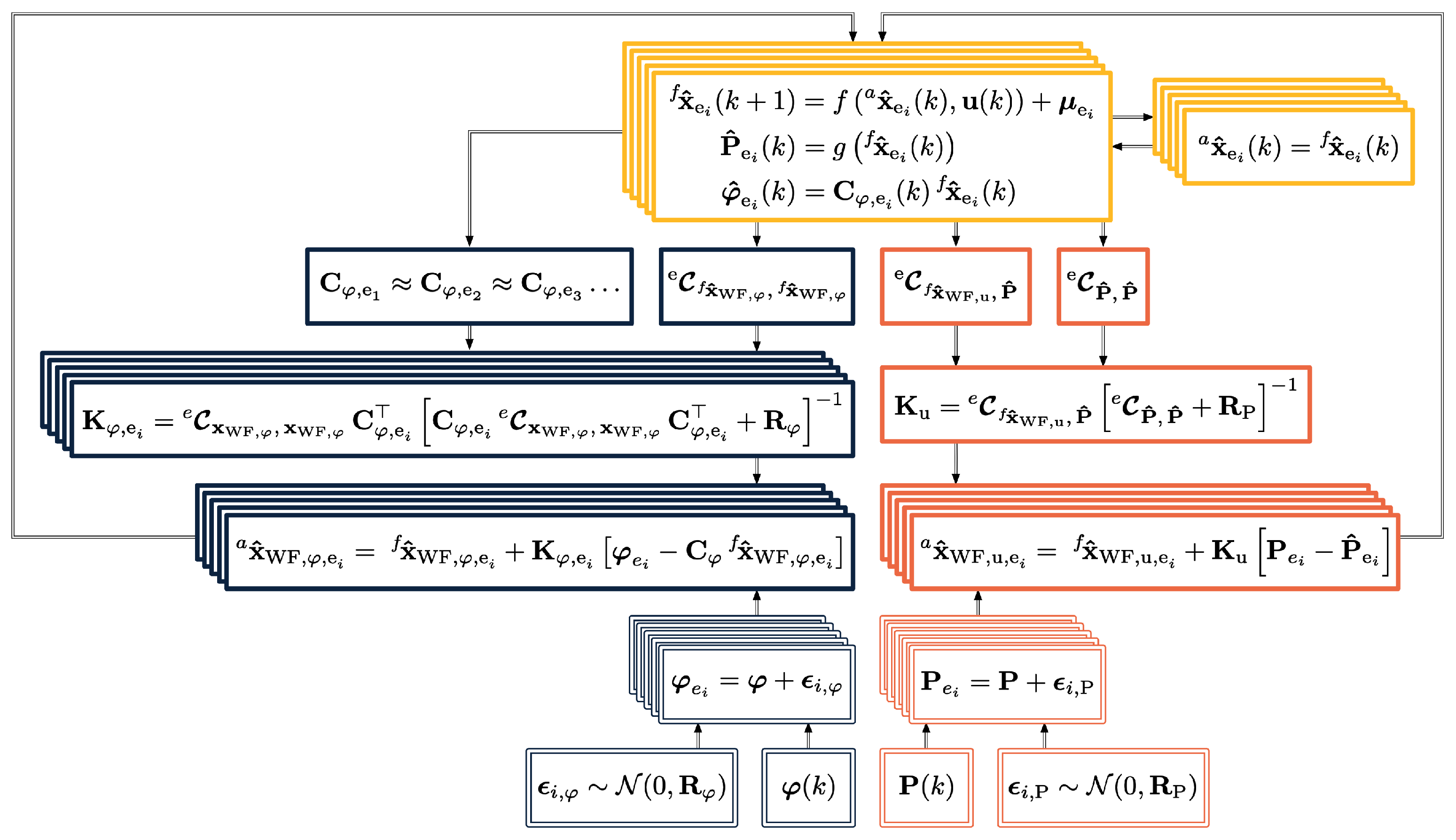
We assume that the wind direction and wind speed are uncorrelated and can be corrected independently. Therefore, the calculation of the Kalman gain matrix is split into K u to correct the wind speed and K φ to correct the wind direction. For the correction of the wind speed, the power generated is used as a nonlinear output. For the wind direction, we assume a direct measurement at the turbine location. Therefore, the output function also varies and K u and K φ have to be calculated in a similar yet different manner. This will be discussed in Section 2.2.1 and Section 2.2.2, respectively. Figure 2 shows a block diagram of the correction from the point of view of a single ensemble.
It visualizes how the estimated wind field states are converted into estimates at the turbine location. The wind direction is determined by a time-varying output matrix, and the wind speed is determined by a nonlinear function which converts the wind speed into power generated. Both estimates are then compared to the polluted measurements. The difference is multiplied with the respective Kalman gain matrix and the forecast states are corrected and fed back into the ensemble. Figure 3 visualizes which calculations are executed for all ensembles and which calculations are used only once. The calculations are mainly based on the EnKF literature and adapted for this case; for more information on the EnKF, see [13,27].

2.2.1. EnKF Correction of the Wind Speed

To calculate the Kalman gain matrix K u , we follow an approach also used in [19], which allows the use of a nonlinear output function. First, the averaged state error matrix f E x ^ WF , u is calculated:
E f x ^ WF , u = 1 n e 1 f x ^ WF , u , e 1 f x ¯ WF , u , f x ^ WF , u , e 2 f x ¯ WF , u , , f x ^ WF , u , e n e f x ¯ WF , u ,
where f x ^ WF , u , e i describes the wind speed estimate of the i-th ensemble and f x ¯ WF , u describes the average across all n e ensembles. The same is calculated for the output of the ensembles:
E P ^ = 1 n e 1 P ^ e 1 P ¯ , P ^ e 2 P ¯ , , P ^ n e P ¯ ,
where P ^ e i denotes the estimation of power generated by the i-th ensemble, which is directly dependent on f x ^ WF , u as shown in Equations (2) and (3). We can now calculate the state-output error correlation covariance matrix, Equation (13), and the output error covariance matrix, Equation (14):
e C f x ^ WF , u , P ^ = E f x ^ WF , u E P ^
e C P ^ , P ^ = E P ^ E P ^ ,
In parallel, the power measurements P from the wind turbines have to be polluted:
P e i = P + ϵ i , P ϵ i , P N ( 0 , R P )
where ϵ i , P is an artificial error with a Gaussian distribution, an average of 0 and the covariance matrix R P . The matrix R P is a parameter which needs to be set based on prior knowledge and tuning. If no random perturbations are added to the measurements, the variance of the analyzed ensembles becomes too low [28]. The wind speed is then corrected as follows:
K u = e C f x ^ WF , u , P ^ e C P ^ , P ^ + R P 1
a x ^ WF , u , e i = f x ^ WF , u , e i + K u P e i P ^ e i ( f x ^ WF , u , e i ) .

2.2.2. EnKF Correction of the Wind Direction
We assume to have a measurement of the wind direction available at the turbine locations. The state error f E x WF , φ is calculated equivalently to Equation (11). Contrary to the wind speed estimation, it is then used to calculate the state error covariance matrix:
e C x WF , φ , x WF , φ = f E x WF , φ f E x WF , φ .
To obtain the relation between the states and the output, the output matrix C φ , e i is needed. It is given by the rows of the weighting matrix W WF ( k , x L ) which combine f x WF , φ to a wind direction estimate at the OP at the rotor plane; see Equation (7). Due to the fact that OPs are slightly differently located in each ensemble, C φ , e i is slightly different in each ensemble. We assume that C φ , e 1 C φ , e 2 C φ , e n e to a degree where the basic assumptions of the EnKF still hold. However, we are diverging from the traditional calculation by generating individual K φ , e i for each ensemble, based on the different C φ , e i matrices. The wind direction measurements φ are also polluted with an error ϵ i , φ N ( 0 , R φ ) , which is equal to the power measurements in Equation (15). As with R P , R φ is a parameter that needs to be set. The resulting analysis step is described by:
K φ , e i = e C x WF , φ , x WF , φ C φ , e i C φ , e i e C x WF , φ , x WF , φ C φ , e i + R φ 1
a x ^ WF , φ , e i = f x ^ WF , φ , e i + K φ , e i φ e i C φ f x ^ WF , φ , e i .
Note how the Equation pair (19) and (20) differs from (16) and (17): Equation (19) uses the state-error-covariance matrix and a linear output matrix, where Equation (16) uses the output-error-covariance matrix and the output-to-state-error-covariance matrix. As a result, Equation (20) corrects based on a linear relation of the output to the estimated state, while Equation (17) compares outputs with a nonlinear relation to the estimated state.
Figure 3 shows the difference between the single K u for the wind speed reduction and the multiple matrices to correct the wind direction. Generally, this approach is not desirable as it requires more calculations and therefore more computational effort. We chose it as we had access to the exact output matrices and were therefore able to reduce the number of approximations in the correction. Furthermore, the later discussed test case is a nine-turbine case, which means that the to-be-inverted part of the Kalman gain calculation is a 9 × 9 matrix, which resembles a manageable computational cost. As the number of turbines grows, a single K u matrix becomes much more desirable.
Figure 3. Block diagram of the correction across all ensembles. The yellow, top boxes describe all ensembles, running in parallel. If no measurements are given, the forecast state is used as an analysis state, and the ensembles diverge further. If measurements are given, the wind speed (orange) and direction (dark blue) states are corrected. The measurements and their perturbations are given at the bottom of the figure with thin double lined frames. Without perturbation, the variance of the ensembles would become too low [28].
Energies 15 08589 g003

2.2.3. Localization

The EnKF works under the premise that enough ensembles are simulated to approximate the correlation among the states and measurements. In order to decrease the number of ensembles needed for the error covariance approximation, prior knowledge of the system can be used to modify the covariance matrices. In practice, this is completed by calculating an additional covariance matrix based on the distance of the state to each other. This covariance matrix is then multiplied with the state-error covariance matrix and the output-to-state error covariance matrix.
e C ˜ x WF , φ , x WF , φ = C x L , x L e C x WF , φ , x WF , φ e C ˜ f x ^ WF , u , P ^ = C x L , x L , T e C f x ^ WF , u , P ^ e C ˜ P ^ , P ^ = C x L , T , x L , T e C P ^ , P ^ ,
where ∘ is the Hadamard product, C x L , x L is the localization covariance between all states, C x L , x L , T is the localization covariance between all states and the OPs at the turbine locations, and C x L , T , x L , T is the localization covariance between the OPs at the turbine locations among each other. As the initial OPs are placed at the turbine location, C x L , T , x L , T and C x L , x L , T are subsets of C x L , x L . To calculate the localization covariance, we follow [29] and use a piece-wise defined polynom with a characteristic cut-off length l. Every element c i , j ( d , l ) of the covariance matrix connecting OP i and OP j is then calculated as follows, based on their distance d to one another:
c i , j ( d , l ) = 1 d = 0 1 4 d l 5 + 1 2 d l 4 + 5 8 d l 3 5 3 d l 2 + 1 0 < d l 1 12 d l 5 1 2 d l 4 5 8 d l 3 5 3 d l 2 5 d l + 4 2 3 d l 1 l < d 2 l 0 2 l < d .
The equation is based on the work of [30], which also offers alternative functions. The state and output covariance matrices in Equations (16) and (19) are subsequently replaced by their modified equivalents, which are defined in Equation (21).

3. Results and Discussion

This section presents the results of the introduced framework. The parameters chosen for the simulation are discussed in Section 3.1. In Section 3.2, we apply the framework to a test case where FLORIDyn is used as both the reference system and the ensemble system. In a second step, Section 3.3 showcases a setup where an LES simulation is used as reference.

3.1. Ensemble Kalman Filter and Localization Parameters

Table 1 lists the used parameters for the EnKF framework and the new weighting method introduced in FLORIDyn. For the other FLORIDyn parameters, see [7]. The number of ensembles defines how well the covariance matrices are approximated, but with every ensemble, also a new FLORIDyn simulation has to run. Preliminary tests suggested that using 50 ensembles yields acceptable results: the estimate becomes noisy for a few ensembles (<20), and the results do not change significantly for higher numbers (tested up to 150). The correction frequency Cf determines how often the framework is called and has to be a multiple of the FLORIDyn simulation frequency, which is set to 0.25 s 1 . The noise on the measurements and states is assumed to be uncorrelated and is therefore described by an identity matrix, which is multiplied by a factor. The factors were chosen based on the variance of the measurements in the LES simulation. The noise perturbation for the wind direction had to be increased to allow for a faster correction. The cut-off length for the localization function was set in accordance to be roughly double the spatial component of the weighted average function, scaled by 10 / 3 , which is motivated by the findings of [31]. The values for the weighted average calculation of the wind speed are inspired by [10] but were modified. The initial values were lower for σ w , t , u and higher for σ w , dw , u . This led to unreasonable weighting areas during major wind direction changes. Therefore, we adapted the values to hold value longer but over shorter downwind distance. The weight for the crosswind distance σ w , cw , u was also set lower, which led to very little interaction between downstream turbines and passing wakes. The value was therefore increased. The wind direction weights are set by manual tuning and intuition: as the wind direction changes, the entire flow field changes, and we can assume a more global effect than with wind speed. If the age of the OPs would not be punished more heavily by the weighting, old wind direction measurements would prohibit a change. We therefore chose to give the wind direction state a wide influence area but a short lifespan. All values should be seen as educated estimates and not necessarily as part of a final parameter set.

3.2. FLORIDyn as Validation Platform

To understand the behavior of the developed algorithm, we first use FLORIDyn itself as a validation platform. This allows us to model flow conditions, which could be hard to generate in high-fidelity simulations. We also can carve out the differences of the FLORIDyn model by itself and FLORIDyn within the EnKF framework. This gives us an idea about the contribution of the EnKF framework. To this end, we consider a nine-turbine case subject to heterogeneous wind speed and wind direction changes. The 3 × 3 wind farm layout is described in Figure 4. All nine DTU 10 MW turbines [32] are placed with equidistant spacing of 900 m , which is roughly equivalent to f i v e turbine diameters. The FLORIDyn model is propagated as described in Equation (8), excluding the noise term. During the 1200 s simulation duration, both the wind direction and speed change heterogeneously throughout the field. The wind direction is initialized with 255 deg and then changes at rates between 0.2 deg s 1 and 0.05 deg s 1 to 280 deg . Figure 4 shows the start and end directions as well as the transitions for the different turbines. The wind speed is changed in a similar manner from 8 to 10 m s 1 at rates between 0.02 and 0.01 m s 2 . Yaw misalignment is not part of the presented case.
Figure 5 depicts the power generated by the center row turbines, T3, T4 and T5. The leftmost turbine, T3, experiences only free stream conditions, and the only change in power generated stems from the increase of wind speed. As the EnKF needs to adapt to the changing wind speed, the predicted power generated trails the reference with a delay of ≈ 10 s . The other two turbines, T4 and T5, are subject to upstream wakes and show a reduction in power generated due to passing wakes during the wind direction change. Both also show that the EnKF predicts the reduction in power generated, but contrary to the prior case, and counter intuitively, the EnKF does not follow the reference simulation but leads it. To understand this effect, we have to look at the state correction: the EnKF has the capability to change the states of shed OPs whereas the FLORIDyn simulation only adds new data to the OPs at the turbine locations. As a result, downstream OPs in the EnKF simulation correct their state while they initially remain unaffected in the FLORIDyn simulation. The effect is that the wake in the EnKF adapts sooner to the new wind direction and crosses the downstream turbines earlier than in the FLORIDyn simulation.
This difference can be seen in Figure 6 where the reference state is compared to the EnKF estimate along with the respective wake locations in white and black. The EnKF simulation shows a similar heterogeneous state distribution as the reference but at a higher value. The resulting difference shows that the EnKF is uniformly at the same or higher value than the reference simulation. The difference plot also shows how the EnKF wake has progressed further south than in the reference case. Figure 7 depicts a similar behavior where the reference states show bigger differences in the background wind speed than the estimated state. The estimated state is more uniform and suggests a more steady change of the wind speed throughout the flow field.
To conclude, the framework creates smoother, low-pass filtered flow fields. The EnKF adds a spatial connection to the FLORIDyn simulation that it, in this implementation, would not have otherwise. This is due to the correction capabilities of the EnKF: the state-error-correlation calculation and the wider localization area connect and change states which are not necessarily connected by the spatio-temporal averaging alone, which is applied in FLORIDyn. This could be changed by narrowing the localization window or by widening the spatio-temporal average influence. The EnKF is furthermore able to track heterogeneous flow field changes.

3.3. SOWFA as Validation Platform

We now consider a more realistic and complex setting, in which we use the developed EnKF FLORIDyn framework to estimate the flow field state during a 60 degree wind direction change. We use a high-fidelity large-eddy simulation performed with SOWFA (Simulator fOr Wind Farm Applications) [33] as ground state. Section 3.3.1 describes the simulation setup and case. The wind speed and direction state estimation results are discussed in Section 3.3.2 and Section 3.3.3, respectively. Section 3.3.4 highlights the influence of spatial weighting on the state correction. Finally, Section 3.3.5 looks at the power generated.

3.3.1. Simulation Case

The wind farm layout is identical to the case discussed in the previous Section 3.2 and is shown in Figure 4. Differences are that the wind direction changes from 255 degrees before t = 600 s to 195 degrees at t = 900 s and afterwards. In SOWFA, the turbines are subject to turbulent inflow at roughly 6 % ambient turbulence intensity and an average wind speed of 8.2 m s 1 . The case has been used in previous FLORIDyn publications, such as [7] and has been described in greater detal in [6]. The SOWFA setup files and output data are available at [34].
For the evaluation, two snapshots are considered: one at t 1 = 600 s , when the wakes are fully developed within the wind farm boundaries, and one at t 2 = 840 s , during the wind direction change. Animations of the full simulation are available at [35] along with data to recreate the flow field plots and power generated.

3.3.2. Wake Location and Estimated Wind Speed

Figure 8 shows the SOWFA flow field at t 1 and t 2 , as well as the SOWFA flow field overlaid with the FLORIDyn OPs and contour lines. The estimated flow field overlaps well with the SOWFA simulation and follows the curved wakes, which are caused by the wind direction change. At its current development stage, FLORIDyn cannot model wake-meandering effects, which are present in the SOWFA flow field.
The estimated FLORIDyn wind speed state is depicted in Figure 9, along with the standard deviation, calculated by the relation between the ensembles. The wind speed estimate is relatively uniform, which is also the case in the SOWFA simulation. Coarser patterns of lower and higher wind speeds can be seen for the three turbine rows. The lower row of T6, T7 and T8 does also show the same lower wind speeds in the SOWFA simulation (consider Figure 4 as reference for the turbine numbering). The standard deviation is below 0.3 m s 1 and does not show a meaningful pattern. During the wind direction change, the standard deviation rises for some downstream areas but remains bounded. The filter properties of spatio-temporal averaging strongly contribute to this result, as small-scale changes are averaged out. The area influenced by the averaging is discussed in detail in Section 3.3.4.

3.3.3. Wind Direction States

The wind direction changes uniformly throughout the wind farm and is not subject to turbulent changes, such as the wind speed. Therefore, noise is only introduced by means of system noise and added measurement noise. If these are chosen too low, the EnKF trusts the model state too much and adapts too slow during the actual state change. Knowledge about the flow field effects is crucial to set the noise magnitude: in this simulation, the wind direction changes with 0.2 deg s 1 . Consequently, the system noise and measurement noise have to be chosen higher. The Gaussian noise is set to 0.75 deg s 1 for both the measurement and the system noise. In steady state, however, the difference between the estimated and true state is minimal. This can be seen in Figure 10.
During the wind direction, the error increases, but due to the introduced noise, the states are corrected and the error remains within small bounds within the wind farm. Outside of the wind farm, little to no corrections are made, and the states keep diverging across all ensembles, which are visible in Figure 11. This is also mirrored in the standard deviation plot in Figure 10, where the areas between the wind turbines, with wake overlap, show the lowest values.

3.3.4. Weighting and Corrections

The previous results underlined the importance of the applied spatio-temporal weighting as well as the localization. The results also show how the weighting changes the way FLORIDyn acts as a simulation and how it defines boundaries to what the EnKF can correct. This section looks at a part of the simulation in detail to quantify and understand these implications.
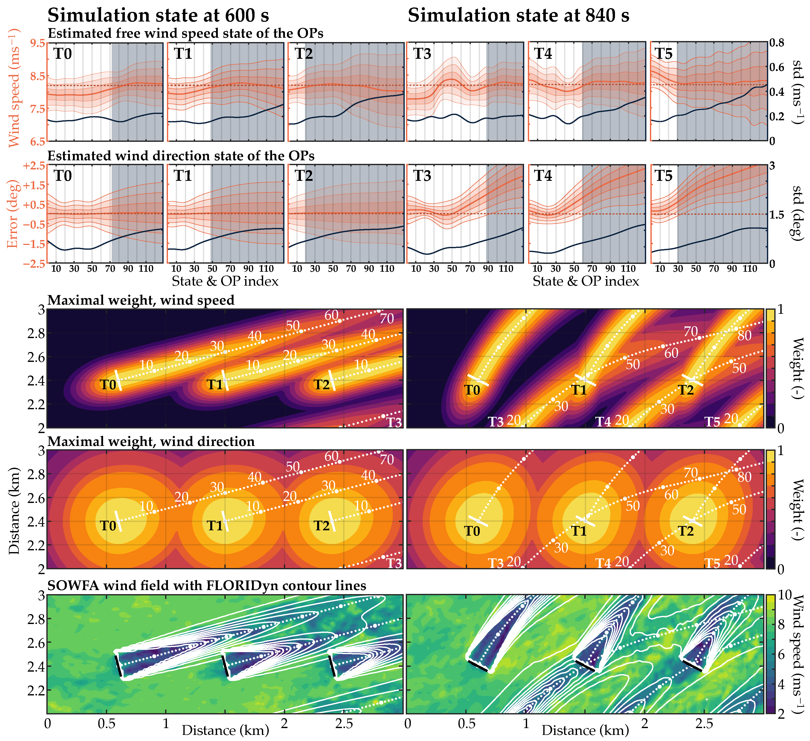
Figure 11 focuses on the upper third of the wind farm area and the states within it. During steady state, the focus lies on the OP states of the turbines T0, T1 and T2. During the wind direction change, the wakes of T0, T1 and T2 leave the observed area, which is why the now more present wakes of T3, T4 and T5 are discussed instead. The displayed metrics from top to bottom are the wind speed state of the OPs, the wind direction state of the OPs, the weights for the wind speed averaging, the weights for the wind direction averaging and the SOWFA flow field overlapped with the FLORIDyn contour lines.
Figure 11. This figure compares the simulation state at the start and during the wind direction change. The top two figure rows visualize the states of all OPs connected to Turbine 0 to 2, at t 1 = 600 s and of all OPs connected to Turbine 3 to 5, at t 2 = 840 s . The figures show the state value of the OPs with 1 , 2 and 3 standard deviations (std) as orange plot and y-axis, and the std alone as black plot and y-axis. A gray area marks the OPs which have left the wind farm boundaries. The x-axis denotes the state index, e.g., 10 relates to the 10th OP. The dotted lines mark a reference value: for the wind direction, this is the true value; for the wind speed, this is the average precursor speed. Below the OP states are three rows of flow field plots. They show a third of the wind farm to allow for a more detailed look. The upper two show the weights used for the weighted average calculation; see Equation (6). These figures also show the state indexes in the wakes of the referenced turbines. The lower row shows the SOWFA flow field overlapped with the contour lines of the FLORIDyn simulation. The dataset [35] provides animations of the state figures for all cases and animations of the flow field.
Energies 15 08589 g011
The wind speed state plots show the estimate of all OP states for three turbines with ± 1 , 2 , 3 standard deviations, as well as a reference line at 8.2 m s 1 . The reference is the mean wind speed across the wake free flow field and only gives an indicator of where the estimate should be. The figures also show the development of the standard deviation separately as a black line. The leftmost states are closest to the turbine, while the rightmost are furthest away. The gray areas indicate where the states leave the wind farm boundaries. Every 10th state (or OP) is marked in the weight plots to aid the interpretation across the plots.
Looking at the wind speed state, it is notable that the standard deviation remains rather constant at or below 0.2 m s 1 within the wind farm bounds, but it then increases as the OPs move farther away from the wind farm region. This means that within the wind farm, the turbines and their measurements keep the variance bounded. As the OPs leave the wind farm bounds, this effect diminishes, and the system noise leads to a divergence of the ensembles. A noticeable difference between the variance of the wind speed states and the later discussed wind direction states is the fact that the wind speed variance does not significantly decrease within the wind farm bounds. This might be expected as the OPs travel past downstream turbines, which act as correcting sensors. The lack of significant correction can be explained by the wind speed weight plot. It shows the influence by the OPs based on the spatio-temporal weighting. Due to the weighting parameters chosen for the wind speed, the area of the influence of an OP has very little overlap with a neighboring wake. The states within a wake therefore tend to develop more independently from other wakes in this wind direction. During the wind direction change, however, the wakes cross and areas of locally lower variance can be seen in the wakes of T3 and T4. These OPs with lower variance are roughly in the direct neighbourhood of the wind turbines T1 and T2. For instance, the OPs of T3 passed T2 60 s (=15 time steps) prior to the snapshot—this reduced the variance of the OPs in the proximity of T2, which then traveled further. The lowered variance can now be seen around OP 70 in the wake of T3.
The reduction of the variance is more dominant with the wind direction states, as the framework assumes a wide area of influence of OPs due to the spatio-temporal weighting. This allows the EnKF to cross-correct from one wake to another. The weighting plot also shows how the wide area of influence decreases with the age of the OPs: OPs close to their turbine have high values, but already, the weights of OP 10 and 20 have decreased significantly. In contrast, the wind speed state weights remain longer at a high level. The wind direction weights therefore encourage corrections of OPs close to the turbines. Thus, the estimated variance decreases in the proximity of the turbines, which is an effect that is also visible in Figure 9. The weights and therefore the connection of measurement-to-state decreases rapidly outside of the wind farm boundaries and the ensembles diverge. During the wind direction change, the states within the wind farm are successfully corrected, while states outside of the wind farm are not. Different from the wind speed states, the wind direction reference resembles the true state, which is why the value is given in absolute difference rather than absolute values.

3.3.5. Power Generated

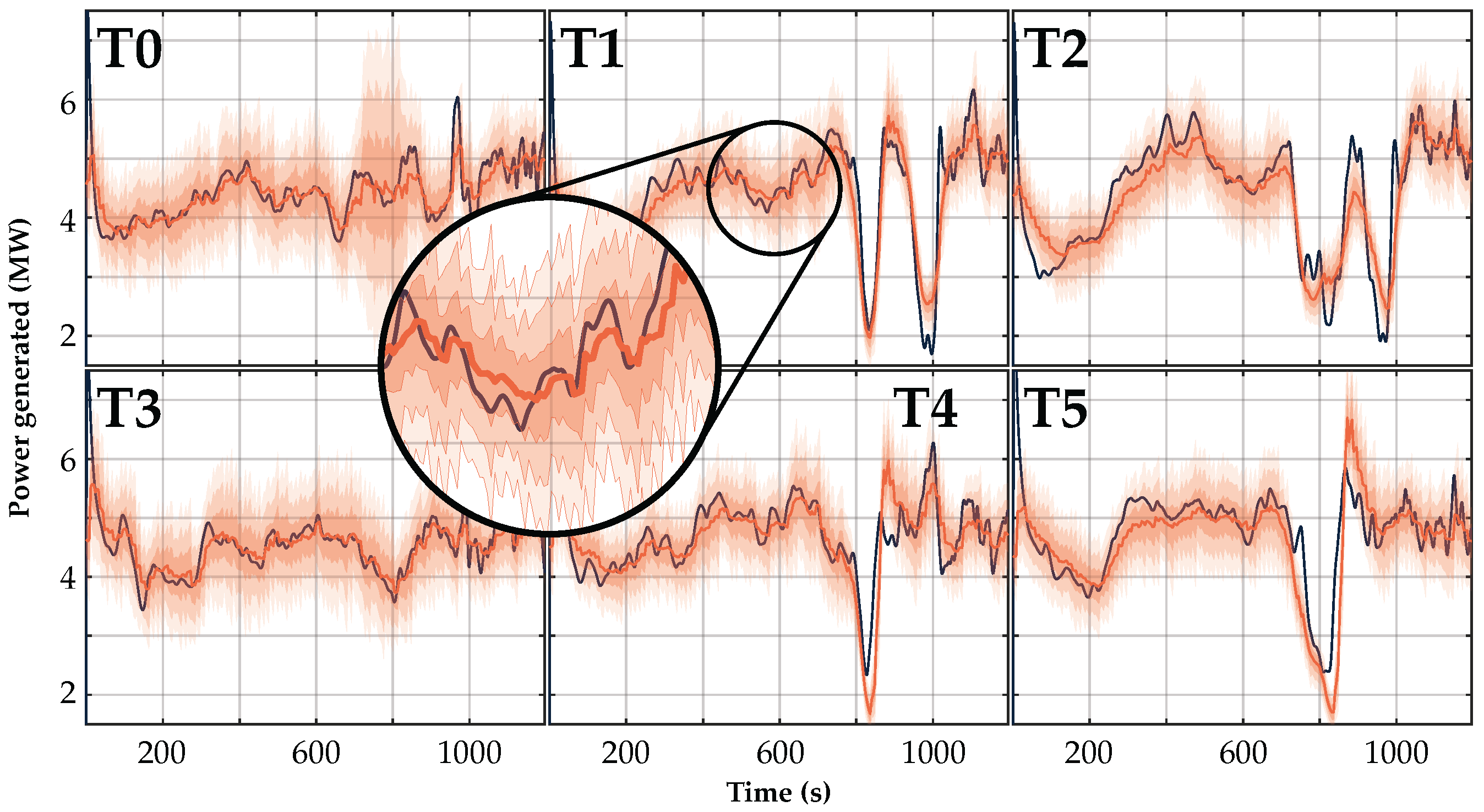
The power generated is not one of the estimated states, but it is inherently linked to them, as shown in Equation (2). Figure 12 depicts the power for six out of the nine turbines in the EnKF framework and SOWFA.
The EnKF estimates the power generated 2700 times during the simulation, 300 values per turbine, every 4 s . Out of these, 73.5 % are within one standard deviation (as estimated by the EnKF) from the SOWFA value, 90.7 % are within two, and 95 % are within three. This does not quite match the Gaussian ideal distribution of 68 % , 95 % and 99.7 % . The mean error lies at 0.0452 MW , about 1 % of the absolute power, while the root-mean squared error lies at 0.4936 MW , which is about 11 % . The small mean error seems to justify the assumption that the surrogate model is error-free on average, which is a necessary assumption for the EnKF. However, the wind speed state noise might be underpredicted. Another metric which is sometimes used for the EnKF is how often the estimate is above or below the measured value. If we understand the true system as another ensemble, the ratio should be about 50 % . For the power generated, this value lies at 53.56 % in favor of an underestimate. Note that these simulations have been run without parameter tuning of the underlying analytical wake model, which would influence these results.
Figure 13 shows a comparison of the same EnKF setup with different correction times, once where the state is corrected every 12 s and once every 60 s . The vertical lines mark the times at which the states are corrected. Note that the time window has been reduced to the last 600 s of the simulation to allow for a clearer picture.
The simulation with the larger correction step shows a much wider variance cone than the simulation with a shorter step, as the ensembles have more time to diverge. Nevertheless, the EnKF is able to track the reference signal under most conditions. A significant decrease of the estimation quality becomes apparent during the wake passing, which is much delayed compared to the SOWFA simulation. In a dynamic wind farm control scenario, this could result in delayed actions which try to improve on a situation that already happened. The delay stems from the fact that FLORIDyn as a surrogate model assumes a steady-state input—during the estimation, the wind direction and speed do become corrected but are then held until the next correction. This could be exchanged for a momentum-driven approach, which continues to change the state based on the previous rate of change. This is subject to further research. Whether such an extension would be valuable can only be judged based on real measurement data and conditions. The implications for this case are that the estimated wakes adapt too slow, and the difference leads to a delayed wake overlap prediction as well as an overshooting of the power signal. The overshooting is also present in some of the power estimates for turbines in the case with a shorter correction step; see T4 or T5 in Figure 12 in a similar context. The dataset [35] contains additional plots for intermediate correction times of 24 , 36 and 48 s .
Lastly, Figure 14 compares the EnKF estimate of the power generated to previous FLORIDyn results in [7]. Previous work used the Immersion and Invariance (I & I) estimator to estimate the effective wind speed based on the rotor speed and generator torque [36]. The base model uses a set wind speed and a prescribed wind direction change. While the base model is unable to mirror the influence of the turbulent wind speed in the reference simulation, it is able to predict the timing of the wake overlap as well as the approximate magnitude. Adding the I & I estimator couples FLORIDyn to the reference simulation and removes the need for a prescribed wind speed. It also allows a close tracking of the power generated. This model, however, still needs a prescribed wind direction. There is furthermore no state correction. The EnKF framework includes both wind speed and direction. It is further able to correct previously generated states and provides certainty bounds for the estimate. On the downside is that this model needs to simulate multiple versions of the same simulation, while previous results were obtained with one simulation.

4. Conclusions

The presented work formulates an ensemble-based wind farm flow field estimation framework which can estimate the background wind speed as well as the wind direction. It is based on the dynamic parametric wind farm model FLORIDyn and utilizes the Ensemble Kalman Filter approach to correct wind speed and direction across the simulation. The approach was tested in a 3 × 3 wind farm case with heterogeneous and changing flow conditions. The results show that the framework is able to follow the flow field changes. Its estimate and corrections strongly depend on the spatio-temporal averaging and localization parameters. These can limit but also enable state corrections and are a vital part of the inner workings of framework. This work also shows that the EnKF can be used to estimate the state of purely Lagrangian particle-based simulations. It further gives an idea on how a state augmentation with the particle position can be avoided by instead projecting the ensembles onto common particle positions. This is under the assumption that the particles across different ensembles are not too far apart.
Given the broader context of wind farm flow control, this work presents an essential building block for a realistic closed-loop dynamic control approach for operational wind farms. Future work will need to address how the framework works in larger wind farms and what the correct parameter choices are under realistic circumstances as well as what framework extensions are necessary.

Author Contributions

Conceptualization, M.B. and J.-W.v.W.; methodology, M.B., D.A. and J.-W.v.W.; software, M.B.; validation, M.B., D.A. and J.-W.v.W.; formal analysis, M.B.; investigation, M.B., D.A. and J.-W.v.W.; resources, J.-W.v.W.; data curation, M.B.; writing—original draft preparation, M.B.; writing—review and editing, M.B., D.A. and J.-W.v.W.; visualization, M.B.; supervision, D.A. and J.-W.v.W.; project administration, M.B.; funding acquisition, J.-W.v.W. All authors have read and agreed to the published version of the manuscript.

Funding

This work is part of the research programme “Robust closed-loop wake steering for large densely spaced wind farms” with project number 17512, which is partly financed by the Dutch Research Council (NWO).

Data Availability Statement

The dataset [35] contains most information needed to recreate the presented plots as well as animations for the full simulation. The SOWFA simulation setup is further explained in [6] and input files as well as output data is available at [34]. The source code is currently not publicly available. If you require specific data, please reach out to Marcus Becker.

Conflicts of Interest

The authors declare no conflict of interest.

Abbreviations

The following abbreviations are frequently used in this manuscript:
EnKFEnsemble Kalman Filter
FLORIDynFLOw Redirection and Induction Dynamics model
WFCWind Farm Control
OPObservation Point
SOWFASimulator fOr Wind Farm Applications

Appendix A. State Space Description

This appendix describes two aspects of the state space description of FLORIDyn more in detail: Appendix A.1 presents the system matrix and the input matrix of the FLORIDyn model. Appendix A.2 then discusses how spatio-temporal weighting is applied in the system matrix.

Appendix A.1. Simple Propagation

The following equations describe the state propagation in the FLORIDyn model and the structure of the matrices:
x L ( k + 1 ) x T ( k + 1 ) x WF ( k + 1 ) = A L , L 0 A L , WF ( x WF ( k ) ) 0 A T , T 0 0 0 A WF , WF x L ( k ) x T ( k ) x WF ( k ) + δ ( x L ( k ) , x T ( k ) , x WF ( k ) ) 0 0 + B L 0 0 0 B T 0 0 0 B WF l T ( k ) x T , 0 ( k ) x WF , 0 ( k ) .
The matrix A L , L is given by
A L , L = A L , L , T 1 0 0 0 0 A L , L , T 2 0 0 0 0 A L , L , T n T 1 0 0 0 0 A L , L , T n T n T · n OP , T · n L × n T · n OP , T · n L
A L , L , T i = 0 0 0 A L , L , OP 1 0 0 0 A L , L , OP 2 0 0 A L , L , OP n OP , T 0 n OP , T · n L × n OP , T · n L
A L , L , OP i = I n L ,
where I n L is the n L × n L identity matrix and n L describes the number of location states per OP. The number of turbines is given by n T and n OP , T describes the number of OPs per turbine. The matrices A T , T and A WF , WF are similar; they only differ in the size of their smallest components: the matrices A T , T , OP and A WF , WF , OP differ in size as the number of stored turbine and wind field states is different.
The matrix A L , WF ( x WF ( k ) ) is described by the same structure than A L , L ; only the smallest component differs:
A L , WF , OP = Δ t cos ( φ OP ) 0 Δ t sin ( φ OP ) 0 0 0 n L × n WF
where Δ t is the time step of the simulation and φ OP is the wind direction at the location of the OP. The number of wind field states is given by n WF . We assume here that the first state is the wind speed.
The input matrices feed inputs into the first OPs of the turbine. For the location data, this is defined as follows:
B L = B L , T 1 0 0 0 0 B L , T 2 0 0 0 0 B L , T n T 1 0 0 0 0 B L , T n T n T · n L · n OP , T × n T · n L
B L , T i = I 3 0 0 0 n L · n OP , T × n L .
We assume here the same use of location states as described in [6,7], where world coordinates are stacked on wake coordinates. The other two input matrices are defined similarly, with the difference that B T , T i and B WF , T i consist only out of an identity matrix in the first rows and not as in B L , T i accompanied by zero columns:
B WF , T i = I n WF 0 n WF · n OP , T × n WF .

Appendix A.2. Weighted Propagation

To apply a spatio-temporal weighting of the wind field states, the time-varying matrix W WF ( k , x L ) is introduced and applied as follows:
A ˜ L , WF = A L , WF ( W WF ( k , x L ) x WF ) W WF ( k , x L ) .
The matrix weights all OP states with respect to a location of interest. The locations of interest in this case are the OPs themselves. As a result, row i contains the weights to sum the influence of all OP states onto OP i. The weights are calculated by Equation (6) and then normalized by the sum of the row. To calculate the time weight, the location of the OP within the state vector can be used along with the time step of the simulation Δ t . If a variable time step is used, this needs to be adapted. In the presented work, only the wind speed and direction are weighted. Weights are denoted as w i , j , u or w i , j , φ , where i is the OP of interest, j is the OP influencing OP i and u or φ represent the wind speed or direction, respectively. Furthermore, we use three wind field states: the wind speed, direction and ambient turbulence intensity. No weighting is applied to the latter but could be implemented in a similar fashion. The matrix W WF is then assembled as follows:
W WF ( k , x L ) = W WF , 1 , 1 ( k , x L ) W WF , 1 , 2 ( k , x L ) W WF , 1 , n OP ( k , x L ) W WF , 2 , 1 ( k , x L ) W WF , 2 , 2 ( k , x L ) W WF , 2 , n OP ( k , x L ) W WF , n OP , 1 ( k , x L ) W WF , n OP , 2 ( k , x L ) W WF , n OP , n OP ( k , x L )
W WF , i , j ( k , x L ) = w i , j , u ( k , x L ) 0 0 0 w i , j , φ ( k , x L ) 0 0 0 w i , j , I 0
w i , j , I 0 = 1 if i = j 0 otherwise .
Note that the row-sum of W WF ( k , x L ) must return a vector of 1 .

References

  1. Fleming, P.; Annoni, J.; Shah, J.J.; Wang, L.; Ananthan, S.; Zhang, Z.; Hutchings, K.; Wang, P.; Chen, W.; Chen, L. Field Test of Wake Steering at an Offshore Wind Farm. Wind. Energy Sci. Discuss. 2017, 2, 229–239. [Google Scholar] [CrossRef] [Green Version]
  2. Kheirabadi, A.C.; Nagamune, R. A Quantitative Review of Wind Farm Control with the Objective of Wind Farm Power Maximization. J. Wind. Eng. Ind. Aerodyn. 2019, 192, 45–73. [Google Scholar] [CrossRef]
  3. van den Broek, M.J.; De Tavernier, D.; Sanderse, B.; van Wingerden, J.W. Adjoint Optimisation for Wind Farm Flow Control with a Free-Vortex Wake Model. Renew. Energy 2022, in press. [Google Scholar] [CrossRef]
  4. Howland, M.F.; Ghate, A.S.; Lele, S.K.; Dabiri, J.O. Optimal Closed-Loop Wake Steering – Part 1: Conventionally Neutral Atmospheric Boundary Layer Conditions. Wind. Energy Sci. 2020, 5, 1315–1338. [Google Scholar] [CrossRef]
  5. Gebraad, P.M.O.; van Wingerden, J.W. A Control-Oriented Dynamic Model for Wakes in Wind Plants. J. Phys. Conf. Ser. 2014, 524, 012186. [Google Scholar] [CrossRef]
  6. Becker, M.; Ritter, B.; Doekemeijer, B.; van der Hoek, D.; Konigorski, U.; Allaerts, D.; van Wingerden, J.W. The Revised FLORIDyn Model: Implementation of Heterogeneous Flow and the Gaussian Wake. Wind. Energy Sci. 2022, 7, 2163–2179. [Google Scholar] [CrossRef]
  7. Becker, M.; Allaerts, D.; van Wingerden, J.W. FLORIDyn—A Dynamic and Flexible Framework for Real-Time Wind Farm Control. J. Phys. Conf. Ser. 2022, 2265, 032103. [Google Scholar] [CrossRef]
  8. Kheirabadi, A.C.; Nagamune, R. A Low-Fidelity Dynamic Wind Farm Model for Simulating Time-Varying Wind Conditions and Floating Platform Motion. Ocean. Eng. 2021, 234, 109313. [Google Scholar] [CrossRef]
  9. Foloppe, B.; Munters, W.; Buckingham, S.; Vandevelde, L.; van Beeck, J. Development of a Dynamic Wake Model Accounting for Wake Advection Delays and Mesoscale Wind Transients. J. Phys. Conf. Ser. 2022, 2265, 022055. [Google Scholar] [CrossRef]
  10. Lejeune, M.; Moens, M.; Chatelain, P. A Meandering-Capturing Wake Model Coupled to Rotor-Based Flow-Sensing for Operational Wind Farm Flow Prediction. Front. Energy Res. 2022, 10, 884068. [Google Scholar] [CrossRef]
  11. Braunbehrens, R.; Schreiber, J.; Bottasso, C.L. Application of an Open-Loop Dynamic Wake Model with High-Frequency SCADA Data. J. Phys. Conf. Ser. 2022, 2265, 022031. [Google Scholar] [CrossRef]
  12. Gebraad, P.M.O.; Fleming, P.A.; van Wingerden, J.W. Wind Turbine Wake Estimation and Control Using FLORIDyn, a Control-Oriented Dynamic Wind Plant Model. In Proceedings of the 2015 American Control Conference (ACC), Chicago, IL, USA, 1–3 July 2015; pp. 1702–1708. [Google Scholar] [CrossRef]
  13. Evensen, G. The Ensemble Kalman Filter: Theoretical Formulation and Practical Implementation. Ocean. Dyn. 2003, 53, 343–367. [Google Scholar] [CrossRef]
  14. Tossavainen, O.P.; Percelay, J.; Tinka, A.; Wu, Q.; Bayen, A.M. Ensemble Kalman Filter Based State Estimation in 2D Shallow Water Equations Using Lagrangian Sensing and State Augmentation. In Proceedings of the 2008 47th IEEE Conference on Decision and Control, Cancún, Mexico, 9–11 December 2008; pp. 1783–1790. [Google Scholar] [CrossRef]
  15. Du, J.; Zhu, J.; Fang, F.; Pain, C.C.; Navon, I.M. Ensemble Data Assimilation Applied to an Adaptive Mesh Ocean Model: Ensemble Data Assimilation Applied to an Adaptive Mesh Ocean Model. Int. J. Numer. Methods Fluids 2016, 82, 997–1009. [Google Scholar] [CrossRef] [Green Version]
  16. Doekemeijer, B.M.; Boersma, S.; Pao, L.Y.; van Wingerden, J.W. Ensemble Kalman Filtering for Wind Field Estimation in Wind Farms. In Proceedings of the 2017 American Control Conference (ACC), Seattle, WA, USA, 24–26 May 2017; pp. 19–24. [Google Scholar] [CrossRef] [Green Version]
  17. Kumar Jain, P.; Mandli, K.; Hoteit, I.; Knio, O.; Dawson, C. Dynamically Adaptive Data-Driven Simulation of Extreme Hydrological Flows. Ocean. Model. 2018, 122, 85–103. [Google Scholar] [CrossRef] [Green Version]
  18. Shapiro, C.R.; Starke, G.M.; Meneveau, C.; Gayme, D.F. A Wake Modeling Paradigm for Wind Farm Design and Control. Energies 2019, 12, 2956. [Google Scholar] [CrossRef] [Green Version]
  19. Sampson, C.; Carrassi, A.; Aydoğdu, A.; Jones, C.K. Ensemble Kalman Filter for Nonconservative Moving Mesh Solvers with a Joint Physics and Mesh Location Update. Q. J. R. Meteorol. Soc. 2021, 147, 1539–1561. [Google Scholar] [CrossRef]
  20. Julier, S.J.; Uhlmann, J.K. New Extension of the Kalman Filter to Nonlinear Systems. Signal Process. Sens. Fusion Target Recognit. 1997, 3086, 182–193. [Google Scholar] [CrossRef]
  21. Talagrand, O.; Courtier, P. Variational Assimilation of Meteorological Observations with the Adjoint Vorticity Equation. I: Theory: VARIATIONAL ASSIMILATION. I: THEORY. Q. J. R. Meteorol. Soc. 1987, 113, 1311–1328. [Google Scholar] [CrossRef]
  22. Wan, E.; Van Der Merwe, R. The Unscented Kalman Filter for Nonlinear Estimation. In Proceedings of the IEEE 2000 Adaptive Systems for Signal Processing, Communications, and Control Symposium (Cat. No.00EX373), Lake Louise, AB, Canada, 1–4 October 2000; pp. 153–158. [Google Scholar] [CrossRef]
  23. Bauweraerts, P.; Meyers, J. Reconstruction of Turbulent Flow Fields from Lidar Measurements Using Large-Eddy Simulation. J. Fluid Mech. 2021, 906, A17. [Google Scholar] [CrossRef]
  24. Skachko, S.; Errera, Q.; Ménard, R.; Christophe, Y.; Chabrillat, S. Comparison of the Ensemble Kalman Filter and 4D-Var Assimilation Methods Using a Stratospheric Tracer Transport Model. Geosci. Model Dev. 2014, 7, 1451–1465. [Google Scholar] [CrossRef] [Green Version]
  25. Bastankhah, M.; Porté-Agel, F. Experimental and Theoretical Study of Wind Turbine Wakes in Yawed Conditions. J. Fluid Mech. 2016, 806, 506–541. [Google Scholar] [CrossRef]
  26. Betz, A. Introduction to the Theory of Flow Machines; Elsevier Science: Amsterdam, The Netherlands, 1966. [Google Scholar]
  27. Evensen, G. Sequential Data Assimilation with a Nonlinear Quasi-Geostrophic Model Using Monte Carlo Methods to Forecast Error Statistics. J. Geophys. Res. Ocean 1994, 99, 10143–10162. [Google Scholar] [CrossRef]
  28. Burgers, G.; van Leeuwen, P.J.; Evensen, G. Analysis Scheme in the Ensemble Kalman Filter. Mon. Weather. Rev. 1998, 126, 1719–1724. [Google Scholar] [CrossRef]
  29. Petrie, R. Localization in the Ensemble Kalman Filter. Master’s. Thesis, University of Reading, Reading, UK, August 2008. [Google Scholar]
  30. Gaspari, G.; Cohn, S.E. Construction of Correlation Functions in Two and Three Dimensions. Q. J. R. Meteorol. Soc. 1999, 125, 723–757. [Google Scholar] [CrossRef]
  31. Lorenc, A.C. The Potential of the Ensemble Kalman Filter for NWP—A Comparison with 4D-Var. Q. J. R. Meteorol. Soc. 2003, 129, 3183–3203. [Google Scholar] [CrossRef]
  32. Bak, C.; Zahle, F.; Bitsche, R.; Kim, T.; Yde, A.; Henriksen, L.C.; Hansen, M.H.; Blasques, J.P.A.A.; Gaunaa, M.; Natarajan, A. The DTU 10-MW Reference Wind Turbine. Available online: https://orbit.dtu.dk/en/publications/the-dtu-10-mw-reference-wind-turbine (accessed on 27 October 2022).
  33. National Renewable Energy Laboratory. Simulator for Offshore Wind Farm Applications. GitHub Repositories 2022. Available online: https://zenodo.org/record/3632051#.Y3tg_n1BxPY (accessed on 28 October 2022).
  34. Becker, M. SOWFA Simulation Setup Belonging to the Paper: The Revised FLORIDyn Model: Implementation of Heterogeneous Flow and the Gaussian Wake. 4TU.ResearchData 2022. Available online: https://data.4tu.nl/articles/dataset/SOWFA_simulation_setup_belonging_to_the_paper_The_revised_FLORIDyn_model_Implementation_of_heterogeneous_flow_and_the_Gaussian_wake/20026406 (accessed on 27 October 2022).
  35. Becker, M. Dataset Belonging to the Paper: Ensemble Based Flow Field Estimation Using the Dynamic Wind Farm Model FLORIDyn. 4TU.ResearchData 2022. Available online: https://data.4tu.nl/articles/dataset/Dataset_belonging_to_the_paper_Ensemble_based_flow_field_estimation_using_the_dynamic_wind_farm_model_FLORIDyn/21215924 (accessed on 3 November 2022).
  36. Liu, Y.; Pamososuryo, A.K.; Ferrari, R.M.G.; van Wingerden, J.W. The Immersion and Invariance Wind Speed Estimator Revisited and New Results. IEEE Control. Syst. Lett. 2022, 6, 361–366. [Google Scholar] [CrossRef]
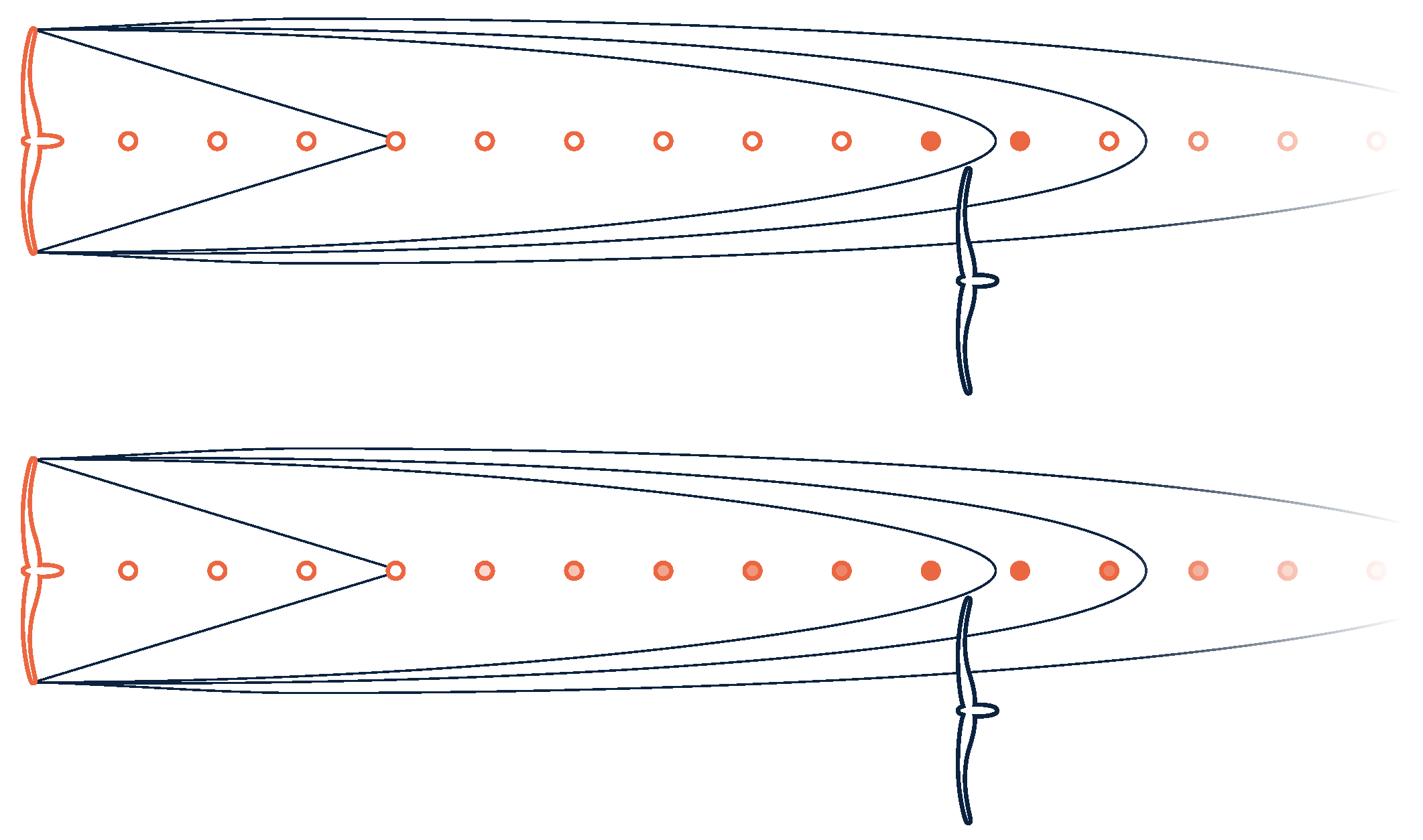
Figure 1. Interaction between OPs and a turbine: the initial case only considered the two closest OPs (upper figure), while the weighted case considers a broader range of OPs (lower figure) to estimate the wind field states at the downstream turbine location.
Energies 15 08589 g001
Figure 2. Block diagram of an ensemble with correction. The left box ( ) describes the state propagation within the ensemble. If no measurements are available, the system keeps progressing the state, and all ensembles diverge due to the influence of noise. The right box ( · ) describes the comparison of the measurements with the estimates and the resulting correction. Elements connected to the wind direction are colored in dark blue, while elements related to the wind speed are colored in orange. Products and functions have a one-line frame; values have a double line frame.
Energies 15 08589 g002
Figure 4. The left figure depicts the wind farm layout which is used in Section 3.2 and Section 3.3, along with the main wind directions in both cases. The right figure depicts the transition between the flow variables for the different turbines during the FLORIDyn reference simulation.
Energies 15 08589 g004
Figure 5. FLORIDyn as reference: the black line shows the FLORIDyn simulation, the orange line shows the estimate with 1 , 2 and 3 standard deviations.
Energies 15 08589 g005
Figure 6. Estimated background flow field wind direction compared to the reference at t = 564 s .
Energies 15 08589 g006
Figure 7. Estimated background flow field wind speed compared to the reference at t = 804 s .
Energies 15 08589 g007
Figure 8. The left figure pair depicts the SOWFA flow field before and during the wind direction change at t 1 = 600 s and t 2 = 840 s , respectively. The right pair superimposes contour lines of the estimated FLORIDyn flow field as well as the OPs.
Energies 15 08589 g008
Figure 9. The estimated effective wind speed flow field is depicted in the left figure pair, once in steady state at t 1 = 600 s and once at t 2 = 840 s , during the wind direction change. The right figure pair shows the respective standard deviation.
Energies 15 08589 g009
Figure 10. The left figure pair shows the difference to the true value and the value extrapolated from the OPs’ wind direction states. A blue color indicates that the extrapolated wind direction is trailing the true value during the direction change. The true values are 255 deg at t 1 = 600 s and 207 deg at t 2 = 840 s , left and right, respectively. The right figure pair shows the standard deviation of the state values based on the variance across the ensembles.
Energies 15 08589 g010
Figure 12. Power generated from six of the nine turbines. This reduction was made as the other turbines are mostly in free stream conditions and do not add more information. The black line depicts the SOWFA simulation as a reference, orange shows the EnKF estimate including 1 , 2 and 3 standard deviation boundaries. As the wind direction changes from t = 600 s to 900 s , T1, T2, T4 and T5 experience a reduction in wind speed due to the passing wakes. This leads to the sudden reduction in the generated power.
Energies 15 08589 g012
Figure 13. Comparison of the predicted power generated by Turbine 1 in an EnKF framework which is updated every 12 s to one which is updated every 60 s . The vertical lines indicate the frequency of correction.
Energies 15 08589 g013
Figure 14. Comparison of the power generated by T1 in different FLORIDyn implementations. The gray area indicates the time window during which the wind direction changes.
Energies 15 08589 g014
Table 1. Parameters used in the Ensemble Kalman Filter framework.
Ensemble Kalman FilterLocalization
n e (-)Cf (s 1 ) l u (m) l φ (m)
50 1 / 12 10 / 3 × 500 10 / 3 × 1000
Noise Per 4 s
R P (MW) R φ (deg) Q u (ms 1 ) Q φ (deg)
0.1 · I n T 3 · I n T 0.4 · I n OP 3 · I n OP
Weighted Average
σ w , dw , u (m) σ w , cw , u (m) σ w , t , u (s) σ w , dw , φ (m) σ w , cw , φ (m) σ w , t , φ (s)
25612625651251250
Publisher’s Note: MDPI stays neutral with regard to jurisdictional claims in published maps and institutional affiliations.