Abstract
The usage of a shunt active power filter (SAPF) is one of the helpful means to mitigate the reactive power and harmonic current of a power grid. The compensation performance of the SAPF is related to the accuracy of the reference voltage extraction from the utility grid, the control stability of the DC-link voltage regulation, and the synchronization between the source voltage and the reference compensation current. To modify the performance of the SAPF for the harmonic compensation, the control strategy of the SAPF reference compensation current based on the recurrent wavelet fuzzy neural network (RWFNN) is proposed in this paper. There are three sections in the proposed control strategy, including the regulated fundamental positive-sequence extraction (section A), DC-link voltage regulation (section B), and calculation of reference compensation current (section C). By regulating the analysis mechanism with the variation of fundamental frequency in the section A, the accurate reference voltage would be obtained. The control stability for the regulation of the DC-link voltage can be accomplished by applying the RWFNN-based controller in the section B. With the synchronized reference voltage in the section A and the estimated control current in the section B, the reference compensation current can be correctly obtained in the section C. From the case studies with the real-time simulator produced by OPAL-RT Technologies Inc., the effectiveness of proposed control strategy for the SAPF reference compensation current can be verified.
1. Introduction
With the widespread usage of nonlinear loads and development of renewable energy in the smart grid, the power-quality disturbances related to the harmonic current and reactive power would be introduced in the power system. These phenomena may result in the misoperation, additional power loss, and reduction in service life for electric devices [1]. Hence, the compensation for the load current to modify the power quality and meet the system requirements is the important issue for the modern power grid. The commonly seen harmonic current mitigation strategies can be divided into the shunt passive power filter and the SAPF. The shunt passive power filter is a traditional and simple way to mitigate the harmonic distortion, which is composed of inductors and capacitors. In recent years, many researches related to the shunt passive filter have focused on the optimal design. By considering the design limitations, the optimal sizing strategy is proposed in [2] to deal with the harmonic distortion for the specific components. In [3], the optimization of size for a novel-type passive filter is developed under non-sinusoidal conditions. To reduce the harmonic disturbances for the demand side, the strategy based on the multi-objective Pareto algorithm is applied in [4] to perform the optimal design of the passive power filter. However, the shunt passive power filter is only useful for the elimination of certain harmonic components. Moreover, the shunt passive power filter may lead to the series or parallel resonance with the system impedance. Due to the characteristics of the dynamic compensation for the time-varying harmonic, the system regulation for the reactive power, the flexible tuning for the specific harmonic components, and the improvement of power factor, the SAPF has become the mainstream strategy for the regulation of power quality [5].
From the research literature, it is found that many effective methods have been proposed to implement the control of the SAPF, including the calculation of the reference compensation current, the phase synchronization for the SAPF compensation, the regulation of the DC-link voltage, the detection of fundamental and harmonic components, etc. In general, many researches apply the instantaneous reactive power compensation control technique (p-q method) for the control of the SAPF [6]. However, the performance of the p-q method may be deteriorated by the deviation of the power system frequency, interharmonics, and distorted source voltage. To solve the drawbacks of the traditional p-q method, the method based on sliding discrete Fourier transform (DFT) is used in [7] to separate the fundamental positive-sequence and harmonic components. Due to the requirement of at least one complete cycle for the calculation of harmonics, the sliding DFT method would suffer from the problem of delayed compensation response. The second-order generalized integrator combined with a comb filter and the instantaneous reactive power compensation theory are applied in [8] to perform the extraction of the phase angle, system frequency, and positive/negative sequences of fundamental component to deal with the limitations of the adaptive notch filters. To improve the compensation response of the SAPF, the algorithm based on an adaptive linear neural network is applied in [5], [9] to perform the real-time harmonic mitigation. Due to the Fourier series-based structure of the adaptive linear neural network, the compensation performance would be interfered with the interharmonics, which are difficult to include in the solution model in advance. The optimized finite impulse response predictor is implemented in [10] to compensate the computation delay, where the optimization of the cost function is performed offline. With the development of intelligent control, many advanced neural network-based strategies have been proposed in the literature. In [11], the recurrent neural network (RNN)-based controller is applied for the approximation of the unknown nonlinear function of the SAPF and modification of the compensation performance. The controller based on fuzzy neural network (FNN) is utilized In [12] to attenuate the effect of arbitrary external disturbances and modeling uncertainties in the process of the SAPF compensation. A compensation method based on recurrent probabilistic fuzzy neural network and global sliding mode control is proposed in [13] to enhance the steady-state and dynamic performance of the SAPF. In [14], the feature selection method with a recurrent neural network is proposed to fit the uncertain function and improve the performance of the conventional global sliding mode control for the SAPF. A self-evolving emotional neural network is applied in [15] to implement a model-free control system to provide fast convergence and global robustness of the SAPF controller. From the above-mentioned researches, it is found that the proposals are mainly focused on the improvement of the SAPF compensation accuracy to meet the requirement of the harmonic injection to the power system in IEEE Standard 519-2022 [16]. Therefore, the power system frequency deviation due to the power mismatch between the energy source and demand side, interharmonics, and distorted source voltage is usually not considered in the solution procedure of the SAPF compensation. In this way, the inaccurate analysis for the reference compensation current and the error of the phase synchronization would be introduced and deteriorate the performance of the SAPF.
In this paper, the control strategy of the reference compensation current with the RWFNN is proposed to perform the accurate fundamental positive-sequence extraction and regulation of the DC-link voltage even when the deviation of power system frequency, distorted source voltage, and interharmonics are present. The main characteristics of the proposed control strategy can be summarized as follows.
- (1)
- The correct synchronization phase angle can be obtained under the conditions of the power-quality disturbances by regulating the analysis matrix for the fundamental positive-sequence component.
- (2)
- The DC-link voltage can be rapidly regulated with the proposed solution mechanism in the load variation.
- (3)
- The accurate value of the reference compensation current can be calculated with the regulated extraction process of the fundamental positive-sequence component and correct phase synchronization even if the deviation of the power system frequency, distorted source voltage, and interharmonics are present.
- (4)
- The parameters of the RWFNN-based controller can be conveniently regulated followed by the requirement of IEEE Standard 519-2022.
The organization of this paper can be listed as follows. In Section 2, the proposed control strategy of the reference compensation current based on the RWFNN controller is introduced, including the fundamental positive-sequence extraction, the calculation of the synchronization phase, the regulation of the DC-link voltage, and the calculation of the reference compensation current. Several comprehensive case studies with a real-time simulator are performed in Section 3 to examine the effectiveness of the proposed control strategy for the SAPF.
2. Proposed Control Strategy of Reference Compensation Current
Figure 1 displays the proposed control strategy of the reference compensation current for the three-phase SAPF based on the RWFNN controller, where Vdc represents the DC-link voltage of the SAPF capacitor, Zs is the line impedance between the load and the power source, Ls is the line inductance between the voltage source inverter (VSI)-based SAPF and the power grid, ILa, ILb, and ILc represent the currents of the nonlinear load extracted from the voltage source Va, Vb, and Vc, In is the current through the neutral line, IC (including ICa, ICb, ICc, and ICn for a, b, c, and neutral phases) is the compensation current from the SAPF, and the superscript * indicates the desired command. The proposed SAPF control strategy can be separated into three sections including the regulated fundamental positive-sequence extraction (section A), the DC-link voltage regulation (section B), and calculation of the reference compensation current (section C).
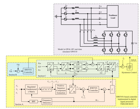
Figure 1.
Proposed control strategy of reference compensation current.
2.1. Section A—Regulated Fundamental Positive-Sequence Extraction
To reduce the interference of the distorted components for the SAPF compensation, the positive-sequence component from the fundamental voltage is calculated in section A. For a voltage Vp (p = a, b, c), the discrete-time signal Vp(n) of the N samples based on the time interval can be expressed with the H sinusoidal components in Equation (1).
where is the amplitude of hth harmonic at phase p, is the hth harmonic phase angle at phase p, and is the angular frequency of the fundamental component. To apply the proposed technique, the model in Equation (1) can be presented in Equation (2).
where is the complex amplitude, , and # expresses the calculation of the complex conjugate. For the N sampled data, Equation (3) can be obtained. In Equation (3), the regulated Vandermonde matrix X can be updated based on the next samples of the power signal. After obtaining the fundamental frequency with the detection method and band-pass filter (BPF) in [17], the complex amplitude A can be obtained via the minimization of the estimated squared error between the practical sample, Vp(n), and the estimated sample, , as displayed in Equation (4).
Then, the estimated value of the complex amplitude can be obtained as
where T represents the transpose of the matrix. The hth harmonic amplitude and phase angle at phase p can be solved from the modulus and argument of the complex amplitude, as listed in Equation (6).
In this way, the fundamental voltage signal Vp_1 at phase p can be synthesized. After the extraction of the positive-sequence component in the fundamental voltage, the RWFNN controller is applied to resolve the referenced phase angle for synchronization θ by regulating the variation between the fundamental quadrature-axis voltage and the reference one .
2.2. Section B—DC-Link Voltage Regulation
2.2.1. Structure of RWFNN-Based Controller
Due to the stable and robust performance in the real-time control, the RWFNN is adopted in this paper to improve the estimation accuracy and control response of the parameter perturbations and achieve the real-time compensation for the uncertain control system [18], [19]. The structure of the RWFNN controller applied for the SAPF compensation is displayed in Figure 2, including Layer 1 (input layer), Layer 2 (membership layer), Layer 3 (wavelet layer), Layer 4 (rule layer), and Layer 5 (output layer). The illustrations and the signal propagation between layers in the RWFNN controller are addressed as follows.
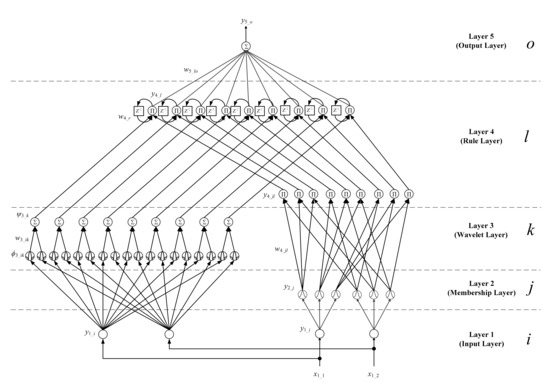
Figure 2.
Structure of RWFNN [18,19].
Layer 1—Input Layer
The input and output of neurons for Layer 1 can be defined as
where and represent the input and output of the ith neuron, and N indicates the iteration index. In this paper, expresses the control error between the reference a-phase fundamental quadrature-axis voltage and instantaneous a-phase fundamental quadrature-axis voltage of controller in section A, expresses the control error between the reference DC-link voltage and instantaneous DC-link voltage of the controller in section B, and is the derivative of .
Layer 2—Membership Layer
The neuron in Layer 2 is a membership function, where the commonly used Gaussian function in the literature [18,19] is applied in this paper. In this way, the jth neuron can be presented by
where is the output of jth neuron for the membership layer, and represent the mean and standard deviations of the Gaussian function in the jth neuron related to the input layer, respectively. Moreover, .
Layer 3—Wavelet Layer
The wavelet function for Layer 3 can be presented in (9).
where represents the kth term of the wavelet function output related to the ith neuron, illustrates the summation of the kth term of the wavelet function output, represents the weight of the wavelet layer, and are the dilation and translation parameters of the wavelet function.
Layer 4—Rule Layer
The first step in the rule layer is to multiply the outputs of layer 2, . The output of neuron would be
where is the weight between the jth neuron of Layer 2 and the lth neuron of Layer 4, which is set to be 1 for the proposed controller. The output of rule layer would be solved by multiplying with the outputs of Layer 3, , and recurrent layer , as given in (12), where represents the recurrent weight.
Layer 5—Output Layer
Then, the defuzzification of Layer 5 can be represented with
where is the weight between Layer 4 and Layer 5, and is the output of RWFNN.
2.2.2. Learning Process of RWFNN-Based Controller
The supervised gradient descent method is applied to update the weights and the related parameters of the RWFNN controller. For the controls in the regulated fundamental positive-sequence extraction (section A) and DC-link voltage regulation (section B), the objective function O(N) can be defined in Equations (14) and (15), respectively.
where e(N) is the estimation error of the RWFNN controller at the discrete time N for the learning process. In this way, the learning process can be listed in the following.
Layer 5—Output Layer
The propagated error term in the Layer 5 for sections A and B can be given by
Then, the weight between Layer 4 and Layer 5 can be updated with Equations (18) and (19). The detailed derivation can be found in [17].
where is the learning rate for Layer 5.
Layer 4—Rule Layer
For Layer 4, the propagated errors can be given in Equations (20)–(22) [17].
where is the learning rate for Layer 4.
Layer 2—Membership Layer
The error of Layer 2 can be represented in Equation (23). The updating amount for the mean of the Gaussian function can be given in Equation (24) based on the chain rule, where indicates the learning rate of [17].
The updating terms of the standard deviation can be represented in Equation (25), where indicates the learning rate [17].
In this way, the mean and standard deviation of the Gaussian function for the Nth discrete sample would be updated, as shown in Equations (26) and (27).
Since it is difficult to resolve the exact values for the Jacobian calculations of and , the error adaptation laws in Equations (28) and (29) are applied to replace the Jacobian term [17].
where and are the first derivatives of the reference a-phase quadrature-axis component for the fundamental voltage and the instantaneous a-phase quadrature-axis component for the fundamental voltage in the section-A controller, and are the first derivatives of the reference DC-link voltage and the instantaneous DC-link voltage in the section-B controller, respectively.
2.3. Section C—Calculation for Reference Compensation Current
From the referenced synchronization phase angle θ obtained in section A, the nonlinear load currents for the three phases ILa, ILb, and ILc are transformed to the direct-axis and quadrature-axis currents Id and Iq. The two low-pass filters (LPF) with the s-domain transfer function F(s) in Equation (30) are applied to extract the DC component of Id and Iq, where the cut-off angular frequency ω is set to be 20π rad/s, the damping ratio λ is set to be 0.7, and the value of gain G is 1.
Then, the direct-quadrature-axis harmonic current components can be obtained by subtracting the DC components from Id and Iq. The control current from the output of the RWFNN controller in section B is used to preserve the DC-link voltage of the SAPF. After the transformation to the abc-axis components, the compensation current is compared to the reference compensation current to generate the control commands for the VSI-based SAPF.
3. Case Studies
To examine the performance of the proposed compensation mechanism for the SAPF, several case studies are implemented in this section based on a real-time simulator numbered OP4510 and RT-LAB environment. Figure 3 depicted the experimental configuration with the OP4510 in this paper. The entire circuit of Figure 1 except the SAPF controller is modeled in the host computer and delivered to the OP4510 via TCP/IP (Transmission Control Protocol/Internet Protocol). The traditional p-q method [6], sliding DFT [7], RNN [11], FNN [12], and proposed control methods are implemented in the digital signal processor TMS320F28335 produced by Texas Instruments for performance comparison through the JTAG (Joint Test Action Group) interface. In order to examine the effectiveness of the proposed RWFNN structure, two modified controllers with the same control procedure in Figure 1 only by replacement of the RWFNN with RNN in [11] and FNN in [12] are applied and implemented. For the implementation simplicity of the digital signal processor, the membership functions with three levels (low, medium, and high) are utilized for the input. This would introduce 3 × 3 = 9 rules for the complete rule connection. By observing the RWFNN structure in Figure 2, there are nine wavelet functions corresponding to the number of rules used. As a result, the implemented RWFNN controller would include 2, 6, 9, 9, 1 nodes for the five layers, respectively. The related parameters for the compared controllers would be fine-tuned as accurately as possible. In general, it is difficult to obtain the specific values of the parameters for the all-neural network-based controllers with the mathematical derivation. The parameters for the RNN, FNN, and RWFNN-based controllers are determined with the experimentation, where the initial values of the parameters are set small and updated to the suitable ones with satisfactory control response [15]. The parameters of the test system are displayed in Table 1. The two indices used to evaluate the performance of the SAPF represented in Equations (31) and (32) are the total harmonic current distortion (THDI) and the unbalance rate (UR) defined in IEEE Standards 519-2022 and 1159-2019 [20], where I1 and IRMS are the fundamental and root-mean-squared (RMS) components of the source current, respectively, IPOS and INEG are the current magnitude of the positive-sequence and negative-sequence components.
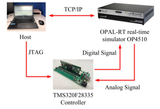
Figure 3.
Experimental configuration with real-time simulator.

Table 1.
System parameters for experiments.
3.1. Case 1—Unbalanced Harmonic Distortion under Nominal Source Voltage
For the first case, the power source in Figure 1 provides the nominal voltage for the unbalanced harmonic and interharmonic loads, which include impedances of (110 Ω + 70 mH) in phase a, (250 Ω + 100 mH) in phase b, (90 Ω + 90 mH) in phase c, and a three-phase pulse-width-modulation VSI-fed AC adjustable speed drive with a motor operating frequency around 50 Hz. To mitigate the harmonic distortion, the SAPF is connected at 0.05 sec to perform the current compensation. The experimental results before compensation, with the traditional p-q method, sliding DFT, RNN, FNN, and proposed control procedure are depicted in Figure 4, Figure 5, Figure 6, Figure 7, Figure 8 and Figure 9 and Table 2. From the experimental results, it is revealed that the proposed compensation method can maintain power quality under unbalanced harmonic and interharmonic distortion with superior performance over others. From Table 2, it is also showed that the proposed control mechanism can significantly reduce the harmonic distortion, which meets the 5%-THDI maximum limitation of IEEE Standard 519-2022, and system unbalance. In this case, the obtained results from the traditional p-q method and sliding DFT would be interfered with the interharmonic current. For the sliding DFT, it is necessary to apply a higher frequency resolution for the correct harmonic compensation. However, it is difficult to determine the suitable frequency resolution for sliding DFT under the time-varying interharmonic disturbance. As a result, the improvement of harmonic distortion and unbalance with the sliding DFT is not significant. Even though the RNN and FNN-based strategies can meet the requirement of IEEE Standard 519-2022, the lower THDI and UR can be obtained with the proposed compensation method. Since RNN and FNN applied the same control mechanism of Figure 1 only by the replacement of the RWFNN, harmonic distortion and unbalance can be effectively reduced by comparing them with the traditional p-q method and sliding DFT. The effectiveness of proposed solution procedure in Figure 1 can be verified.
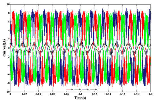
Figure 4.
Source current before SAPF compensation for case 1.
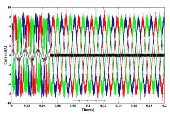
Figure 5.
Experimental result of the traditional p-q method for case 1.
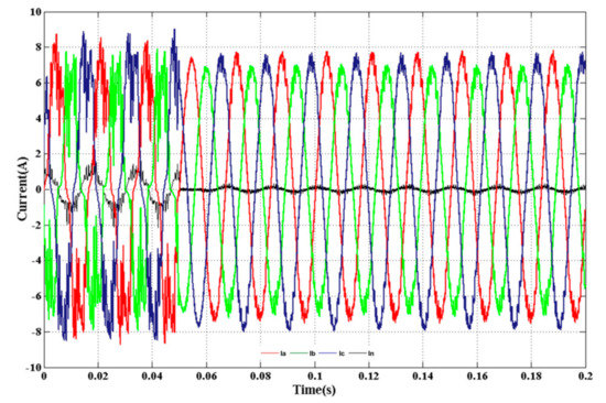
Figure 6.
Experimental result of the sliding DFT for case 1.
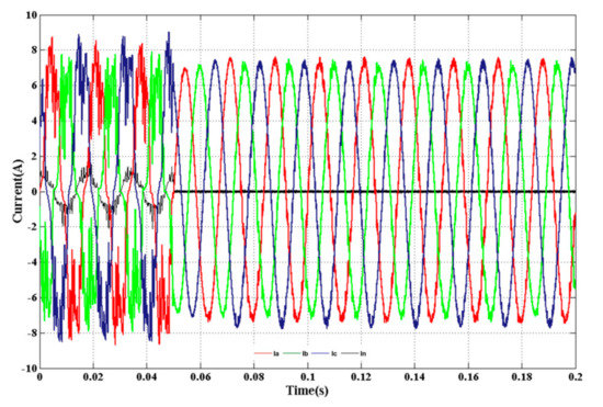
Figure 7.
Experimental result of the RNN for case 1.
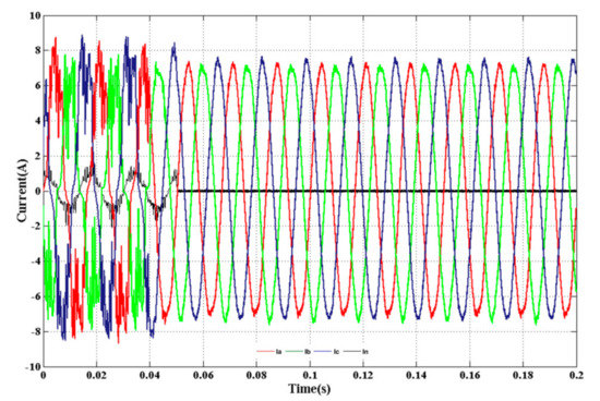
Figure 8.
Experimental result of the FNN for case 1.
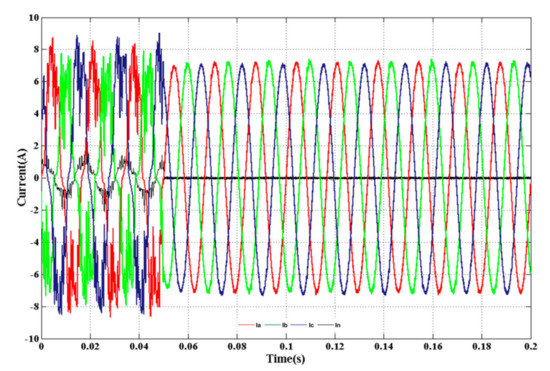
Figure 9.
Experimental result of the proposed control mechanism for case 1.
Table 2.
Experimental results for case 1.
3.2. Case 2—Unbalanced Harmonic Distortion under Power System Frequency Deviation
In this case, the power system frequency of the power source is set in the RT-LAB environment to make the deviation from 60 Hz to 59.7 Hz at the beginning. According to the detection method applied in the section A, the relative estimation error for the power system frequency is within 0.02%. The compensation results without and with the mentioned compensation strategies are depicted in Figure 10, Figure 11, Figure 12, Figure 13, Figure 14 and Figure 15 and Table 3.
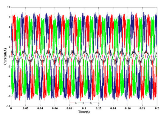
Figure 10.
Source current before SAPF compensation for case 2.
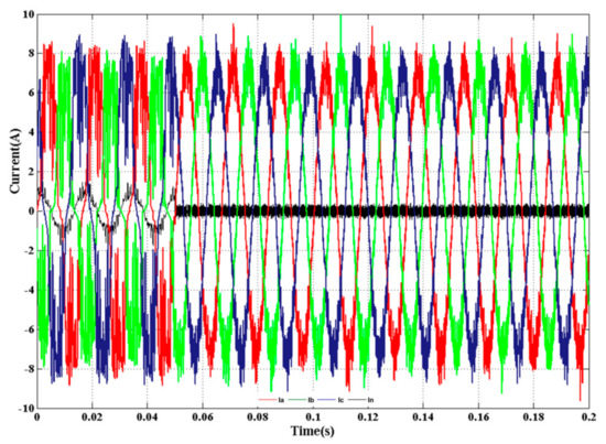
Figure 11.
Experimental result of the traditional p-q method for case 2.
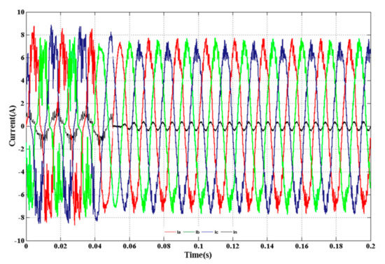
Figure 12.
Experimental result of the sliding DFT for case 2.
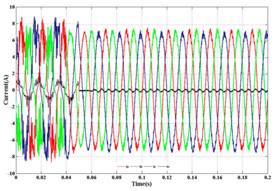
Figure 13.
Experimental result of the RNN for case 2.
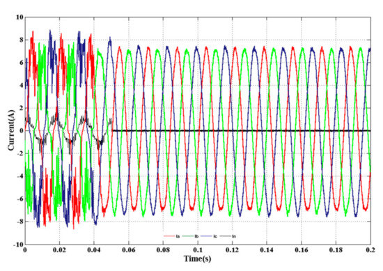
Figure 14.
Experimental result of the FNN for case 2.
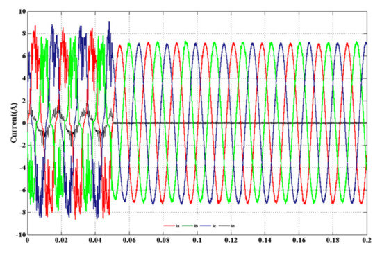
Figure 15.
Experimental result of the proposed control mechanism for case 2.
Table 3.
Experimental results for case 2.
The SAPF is turned on and connected to the power system at 0.05 sec. By oberserving the testing results, it is reazlied that the sliding DFT would be interfered with the deviation of the power system frequency, which leads to a higher evaluation indices in this case compared to case 1. For the traditional p-q method, the power system frequency deviation would not significantly influence the compensation result. The compensation performance of RNN and FNN-based SAPF would not be deteriorated in this case since the same control mechanism of Figure 1 is used. It is displayed that the frequency detection process and regulated fundamental positive-sequence extraction proposed in this paper can effectively enhance the SAPF’s compensation performance. By observing the experimental results of Figure 13, Figure 14 and Figure 15 and Table 3, it is verified that the proposed RWFNN control mechanism can achieve the lower THDI and UR values compared to other approaches.
3.3. Case 3—Unbalanced Harmonic Distortion under Distorted Source Voltage
To realize the influence of the distorted source voltage to the compensation results of the SAPF, the 3rd harmonic with a 30% fundamental magnitude and the 5th harmonic with a 20% fundamental magnitude are included in the source voltage. This distorted source voltage provides electric energy to the 25.63%-THDI and 10.68%-UR nonlinear load. The testing results without and with the compared compensation strategies at 0.05 sec are shown in Figure 16, Figure 17, Figure 18, Figure 19, Figure 20 and Figure 21 and Table 4. It is found that the compensation performance of the traditional p-q method and sliding DFT would be seriously deteriorated in this case. The reason to make such results comes from the usage of the pure sinusoidal source voltage in the synchronization. The distorted source voltage would significantly interfere with the calculation of the reference compensation current of the SAPF. On the contrary, the proposed solution procedure in Figure 1 can effectively prevent the interference of the distorted source voltage, as depicted in Figure 19, Figure 20 and Figure 21 and Table 4. Moreover, the proposed RWFNN-based control strategy can obtain better compensation results. Under the same control mechanism of Figure 1, the compensation results with RNN and FNN can meet the requirements of IEEE Standard 519-2022 to reduce the harmonic distortion and unbalance.
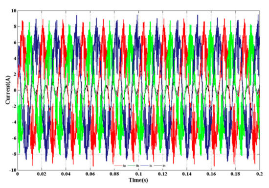
Figure 16.
Source current before SAPF compensation for case 3.
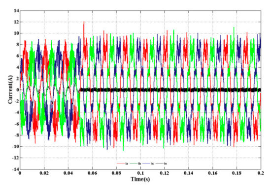
Figure 17.
Experimental result of the traditional p-q method for case 3.
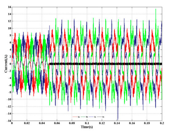
Figure 18.
Experimental result of the sliding DFT for case 3.
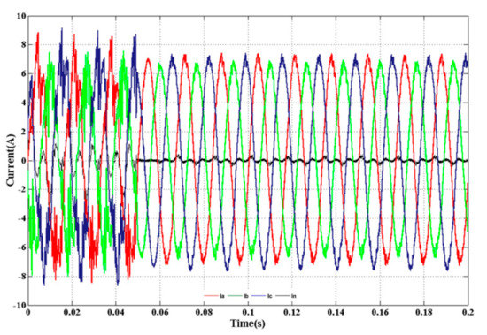
Figure 19.
Experimental result of the RNN for case 3.
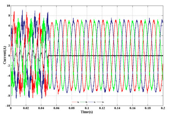
Figure 20.
Experimental result of the FNN for case 3.
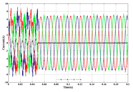
Figure 21.
Experimental result of the proposed control mechanism for case 3.
Table 4.
Experimental results for case 3.
3.4. Case 4—Load Variation for DC-Link Voltage Regulation
Since the instantaneous power varaition of the load would lead to the vibration of DC-link voltage, the performance examination of the addressed control methods would be verified. For case 4, the power variation of the nonlinear load from the light load to the heavy load is present at 1.5 sec, as shown in Figure 22. During the whole simulation time, the SAPF with the different control methods is always connected to the system. From the simulation results in Figure 23, Figure 24, Figure 25, Figure 26, Figure 27 and Figure 28 and Table 5, it is displayed that the proposed RWFNN-based controller can significantly achieve the regulation of the DC-link voltage. On the contrary, the traditional p-q method and the sliding DFT controller would result in the deviation of the DC-link voltage since the power variation of the nonlinear load is present. In addition, the performance for the response time and control stability (from overshoot to undershoot) of the proposed control mechanism is superior to others, as depicted in Figure 28 and Table 5.
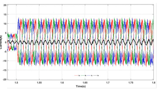
Figure 22.
Power variation of nonlinear load.
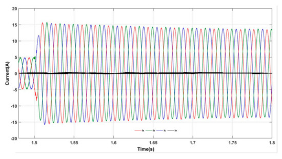
Figure 23.
Experimental result of the traditional p-q method for case 4.
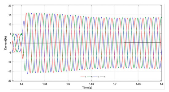
Figure 24.
Experimental result of the sliding DFT for case 4.
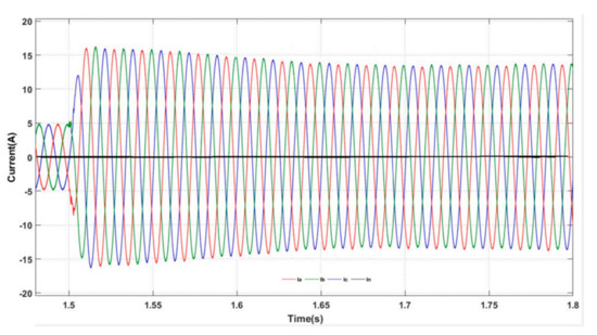
Figure 25.
Experimental result of the RNN for case 4.
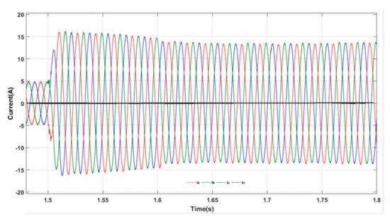
Figure 26.
Experimental result of the FNN for case 4.
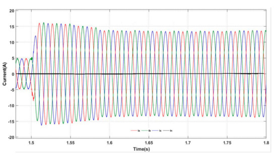
Figure 27.
Experimental result of the proposed control mechanism for case 4.
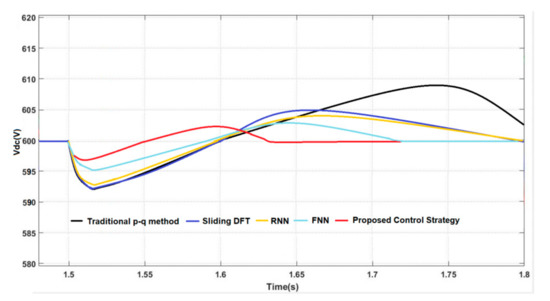
Figure 28.
Regulation results of DC-link voltage.
Table 5.
Comparison for transient response.
4. Conclusions
In this paper, the control mechanism for the SAPF reference compensation current based on the RWFNN controller is proposed to modify the harmonic compensation performance under the disturbances of interharmonics, unbalance, power system frequency deviation, and load variation. Through the process of regulated fundamental positive-sequence extraction, the correct phase synchronization can be achieved even though the power system frequency deviation or distorted source voltage is present. With the regulation process of the DC-link voltage and synchronization of the phase angle, the reference compensation current would be accurately calculated under the conditions of the unbalanced interharmonic or load variation. In comparison with the traditional p-q method and sliding DFT, the solution procedure proposed in Figure 1 can effectively prevent the interference of power-quality disturbances. From the experimental result in Table 5, it is realized that the compensation response of the proposed control mechanism is superior to others. In addition, the compensation results of the proposed control strategy also can meet the requirements of IEEE Standard 519-2022.
Author Contributions
Conceptualization, C.-I.C.; data curation, Y.-C.C.; investigation, C.-I.C.; methodology, C.-I.C.; resources, C.-H.C.; software, Y.-C.C.; validation, C.-I.C.; visualization, C.-H.C.; writing—original draft, C.-I.C.; writing—review and editing, C.-I.C. All authors have read and agreed to the published version of the manuscript.
Funding
This research was funded by the Ministry of Science and Technologies, grant number MOST 111-2628-E-008-004-MY3 and MOST 111-3116-F-008-003, and the Institute of Nuclear Energy Research, grant number 111A012.
Acknowledgments
The authors would like to thank the reviewers for the helpful comments and suggestions for the improvement of the presentation.
Conflicts of Interest
The authors declare no conflict of interest.
Abbreviations
| SAPF | shunt active power filter |
| RWFNN | recurrent wavelet fuzzy neural network |
| DFT | discrete Fourier transform |
| RNN | recurrent neural network |
| FNN | fuzzy neural network |
| VSI | voltage source inverter |
| BPF | band-pass filter |
| LPF | low-pass filter |
| TCP/IP | Transmission Control Protocol/Internet Protocol |
| JTAG | Joint Test Action Group |
| THDI | total harmonic current distortion |
| UR | unbalance rate |
| RMS | root-mean-squared |
References
- Chen, C.I.; Berutu, S.S.; Chen, Y.C.; Yang, H.C.; Chen, C.H. Regulated Two-Dimensional Deep Convolutional Neural Network-Based Power Quality Classifier for Microgrid. Energies 2022, 15, 2532. [Google Scholar] [CrossRef]
- Menti, A.; Zacharias, T.; Milias-Argitis, J. Optimal sizing and limitations of passive filters in the presence of background harmonic distortion. Electr. Eng. 2009, 91, 89–100. [Google Scholar] [CrossRef]
- Mohamed, I.F.; Abdel Aleem, S.H.E.; Ibrahim, A.M.; Zobaa, A.F. Optimal sizing of C-type passive filters under non-sinusoidal conditions. Energy Technol. Policy. 2014, 1, 35–44. [Google Scholar] [CrossRef]
- Bajaj, M.; Sharma, N.K.; Pushkarna, M.; Malik, H.; Alotaibi, M.A.; Almutairi, A. Optimal Design of Passive Power Filter Using Multi-Objective Pareto-Based Firefly Algorithm and Analysis Under Background and Load-Side’s Nonlinearity. IEEE Access 2021, 9, 22724–22744. [Google Scholar] [CrossRef]
- Chen, C.I.; Lan, C.K.; Chen, Y.C.; Chen, C.H. Adaptive Frequency-Based Reference Compensation Current Control Strategy of Shunt Active Power Filter for Unbalanced Nonlinear Loads. Energies 2019, 12, 3080. [Google Scholar] [CrossRef]
- Chauhan, S.K.; Shah, M.C.; Tiwari, R.R.; Tekwani, P.N. Analysis, Design and Digital Implementation of a Shunt Active Power Filter with Different Schemes of Reference Current Generation. IET Power Electron. 2014, 7, 627–639. [Google Scholar] [CrossRef]
- Maza-Ortega, J.M.; Rosendo-Macias, J.A.; Gomez-Exposito, A.; Ceballos-Mannozzi, S.; Barragan-Villarejo, M. Reference Current Computation for Active Power Filters by Running DFT Techniques. IEEE Trans. Power Deliv. 2010, 25, 1986–1995. [Google Scholar] [CrossRef]
- Golla, M.; Thangavel, S.; Simon, S.P.; Padhy, N.P. A Novel Control Scheme using UAPF in an Integrated PV Grid-tied System. IEEE Trans. Power Deliv. 2022, 1–13. [Google Scholar] [CrossRef]
- Kumar, A.; Kumar, P. Power Quality Improvement for Grid-connected PV System Based on Distribution Static Compensator with Fuzzy Logic Controller and UVT/ADALINE-based Least Mean Square Controller. J. Mod. Power Syst. Clean Energy 2021, 9, 1289–1299. [Google Scholar] [CrossRef]
- Kukrer, O.; Komurcugil, H.; Guzman, R.; Vicuna, L.G. A New Control Strategy for Three-Phase Shunt Active Power Filters Based on FIR Prediction. IEEE Trans. Ind. Electron. 2021, 68, 7702–7713. [Google Scholar] [CrossRef]
- Fei, J.; Wang, H. Experimental Investigation of Recurrent Neural Network Fractional-Order Sliding Mode Control of Active Power Filter. IEEE Trans. Circuits Syst. II 2020, 67, 2522–2526. [Google Scholar] [CrossRef]
- Hou, S.; Fei, J.; Chen, C.; Chu, Y. Finite-Time Adaptive Fuzzy-Neural-Network Control of Active Power Filter. IEEE Trans. Power Electron. 2019, 34, 10298–10313. [Google Scholar] [CrossRef]
- Hou, S.; Wang, C.; Chu, Y.; Fei, J. Neural-Observer-Based Terminal Sliding Mode Control: Design and Application. IEEE Trans. Fuzzy Syst. 2022, 30, 4800–4814. [Google Scholar] [CrossRef]
- Hou, S.; Chu, Y.; Fei, J. Intelligent Global Sliding Mode Control Using Recurrent Feature Selection Neural Network for Active Power Filter. IEEE Trans. Ind. Electron. 2021, 68, 7320–7329. [Google Scholar] [CrossRef]
- Chu, Y.; Fu, S.; Hou, S.; Fei, J. Intelligent Terminal Sliding Mode Control of Active Power Filters by Self-evolving Emotional Neural Network. IEEE Trans. Ind. Inform. 2022, in press. [Google Scholar] [CrossRef]
- IEEE Std. 519-2022; IEEE Standard for Harmonic Control in Electric Power Systems. IEEE: Piscataway, NJ, USA, 2022.
- Chen, C.I.; Chen, Y.C.; Chen, C.H.; Chang, Y.R. Voltage Regulation Using Recurrent Wavelet Fuzzy Neural Network-Based Dynamic Voltage Restorer. Energies 2020, 13, 6242. [Google Scholar] [CrossRef]
- Lin, F.J.; Tan, K.H.; Luo, W.C.; Xiao, G.D. Improved LVRT Performance of PV Power Plant Using Recurrent Wavelet Fuzzy Neural Network Control for Weak Grid Conditions. IEEE Access 2020, 8, 69346–69358. [Google Scholar] [CrossRef]
- Liu, S.; Guo, X.; Zhang, L. Robust Adaptive Backstepping Sliding Mode Control for Six-Phase Permanent Magnet Synchronous Motor Using Recurrent Wavelet Fuzzy Neural Network. IEEE Access 2017, 5, 14502–14515. [Google Scholar]
- IEEE Std. 1159-2019; IEEE Recommended Practice for Monitoring Electric Power Quality. IEEE: Piscataway, NJ, USA, 2019.


Publisher’s Note: MDPI stays neutral with regard to jurisdictional claims in published maps and institutional affiliations. |
© 2022 by the authors. Licensee MDPI, Basel, Switzerland. This article is an open access article distributed under the terms and conditions of the Creative Commons Attribution (CC BY) license (https://creativecommons.org/licenses/by/4.0/).