Abstract
A comprehensive review of modelling techniques for the flow-induced vibration (FIV) of bluff bodies is presented. This phenomenology involves bidirectional fluid–structure interaction (FSI) coupled with non-linear dynamics. In addition to experimental investigations of this phenomenon in wind tunnels and water channels, a number of modelling methodologies have become important in the study of various aspects of the FIV response of bluff bodies. This paper reviews three different approaches for the modelling of FIV phenomenology. Firstly, we consider the mathematical (semi-analytical) modelling of various types of FIV responses: namely, vortex-induced vibration (VIV), galloping, and combined VIV-galloping. Secondly, the conventional numerical modelling of FIV phenomenology involving various computational fluid dynamics (CFD) methodologies is described, namely: direct numerical simulation (DNS), large-eddy simulation (LES), detached-eddy simulation (DES), and Reynolds-averaged Navier–Stokes (RANS) modelling. Emergent machine learning (ML) approaches based on the data-driven methods to model FIV phenomenology are also reviewed (e.g., reduced-order modelling and application of deep neural networks). Following on from this survey of different modelling approaches to address the FIV problem, the application of these approaches to a fluid energy harvesting problem is described in order to highlight these various modelling techniques for the prediction of FIV phenomenon for this problem. Finally, the critical challenges and future directions for conventional and data-driven approaches are discussed. So, in summary, we review the key prevailing trends in the modelling and prediction of the full spectrum of FIV phenomena (e.g., VIV, galloping, VIV-galloping), provide a discussion of the current state of the field, present the current capabilities and limitations and recommend future work to address these limitations (knowledge gaps).
1. Introduction
Flow-induced vibration (FIV) of bluff body structures is a classical bidirectional flow–structure interaction problem, which is linked to various fluid dynamics phenomena (e.g., boundary-layer separation, vortex formation and shedding, hydrodynamic loading on the structures) as well as structure vibrations. These phenomena occur widely in various structures (e.g., bridges, transmission lines, marine cables, riser pipes) exposed to wind, tidal waves, or river flow. As a consequence, FIV phenomena have attracted increasing attention over the past few decades owing to complex physics and important practical value [1].
Flow-induced vibration involves the strong interaction between flow and structure. This interaction consists of highly non-linear dynamical phenomena which pose a great challenge for its modelling. FIV itself is also a multi-parameter problem, involving a number of flow properties (e.g., Reynolds number Re, Strouhal number , inflow speed, turbulent intensity), the geometry of the moving body (e.g., cross-sectional shape), and the elasticity of the supporting structure (e.g., mass ratio, damping ratio, spring stiffness). Furthermore, the complete analysis of FIV phenomena must include not only the oscillatory (vibrational) motion of the body (e.g,. displacement, frequency, phase angle), but also the complex dynamics of the flow past the body responsible for this motion (e.g., vortex mode, wake evolution, boundary-layer separation and reattachment). Needless to say, FIV is a very complex physical phenomenon that poses a grand challenge for modelling.
Flow-induced vibration is a general term encompassing various structure oscillations stimulated by the fluid flow, such as vortex-induced vibration, galloping, flutter, buffeting, and wake galloping. Generally speaking, the inducing mechanisms and the response characteristics of these FIV phenomena are distinctive. A key component of research in FIV concerns the underlying mechanisms leading to the structural oscillations—the mechanisms facilitate the identification of the type of FIV and, as a result, lead to improvements in our current understanding of this important physical phenomenon [2].
To study FIV of a bluff body, the most direct and effective approach is to undertake wind-tunnel or water-channel experimental investigations. However, these investigations need to be supplemented with the mathematical or numerical modelling of the phenomenon—this modelling effort provides the required insights and intuition into the physical mechanisms underpinning the observed FIV phenomenon. General modelling methods are based on physical theory or numerical investigations. The main difference between these two approaches concerns the dynamical behavior of fluid—the hydrodynamic forces acting on the structure is either represented (approximated) using a simplified dynamical system model (mathematical modelling) or numerically computed using various approximations of the Navier–Stokes (NS) equations (numerical modelling). In general, mathematical modelling is more efficient and plays a critical role in our understanding of the underlying physical nature of the FIV phenomenon. By contrast, numerical modelling can obtain more accurate predictions of the FIV response and provide much more detailed information of flow field, albeit at much greater computational cost especially for a fully three-dimensional (3D) numerical simulation. In addition to these more traditional approaches for modelling FIV phenomena, there are newly emerging (nascent) machine learning procedures that can potentially be utilized to address the FIV problem. Indeed, ML has been applied recently in the context of fluid dynamics to address a number of different problems of engineering and practical interest [3,4,5].
In terms of practical applications, the suppression of FIV in structures in order to mitigate structural damage has been the dominant area of research. However, in light of an emerging trend toward sustainability goals for clean energy generation in recent years, there is increasing interest in the utilization of FIV phenomena for clean energy production, especially as it relates to the development of small-scale (portable) wind generators—indeed, the energy that can be harnessed from an oscillating body undergoing FIV can be effectively utilized and converted into usable forms of energy, such as electricity, by certain piezoelectric or electromagnetic materials [6,7,8]. In consequence, there is a growing body of research whose objective is to amplify and harness the oscillations of a bluff body immersed in a flow, rather than trying to suppress these oscillations (which is the focus of more traditional research to maintain structural integrity).
This review will focus on providing an extensive and systematic overview of traditional as well as novel (emerging) approaches for modelling FIV phenomena. To this purpose, we elaborate on how these different modelling methodologies can be applied to specific engineering applications of FIV phenomena which we believe will be of interest to both the general and specialist reader. The end goal is to provide a comprehensive survey of traditional (mathematical and numerical) and data-driven (machine-learning) approaches for addressing the modelling of FIV phenomena which we hope will serve as a reference point for both researchers and practitioners (both in and out of the field) not only by providing a categorization of the existing methods, but also providing recommendations for their applicability to various problems. Towards this objective, the application of FIV phenomena to energy harvesting is used as a representative application case to discuss how these various modelling methods can be implemented to address a specific engineering problem. Finally, an outlook focused on the challenges and future directions for research in FIV modelling is provided.
To reiterate, we believe that a comprehensive review of the principal prevailing trends in the modelling and prediction of all aspects of FIV phenomena (e.g., VIV, galloping, VIV-galloping) presented from an integrated and unified perspective will provide an important impetus to advance our current state of knowledge in this field. Indeed, we expect that this new clarity can improve our current understanding of FIV phenomena and enable robust progress—indeed, in this work, we present current limitations in the modelling of FIV phenomena and, based on these limitations, we propose various settings within the current modelling progress of FIV phenomena that are under-explored but are potentially critical for real-world applications of FIV (e.g., energy harvesting).
The paper is organized as follows. Section 2 provides the fundamental concepts and necessary background for the general reader to understand FIV phenomena which includes key definitions and the classification and the characteristics of critical response characteristics of FIV. Two conventional (traditional) modelling approaches based on mathematical (semi-analytical) modelling and numerical modelling (Navier–Stokes equations) are summarized in Section 3 and Section 4. This is followed by a survey of the use of emerging artificial intelligence (or data-driven) approaches for modelling FIV phenomena in Section 5. Section 6 describes the application of these modelling approaches to an FIV energy harvester. Finally, the challenges and prospects of FIV modelling (and their applications to energy harvesting) and new research directions are discussed in Section 7.
2. Fundamental Concepts and Background of FIV
Flow-induced vibration refers to the alternating motion of a structure due to the aerodynamic force exerted by a moving fluid over the body surface. The flow regime that results is significantly affected by this structural motion—in consequence, FIV is a classical bidirectional FSI problem.
In 1977, Blevins [9] first coined the term “FIV” and classified FIV mechanisms according to steady and unsteady flow conditions. In a steady flow, the interaction of the fluid and structure always has a fixed pattern which is predictable. On the other hand, an unsteady FSI can involve either random patterns dominated by transient forces (e.g., turbulence and sudden changes of the flow), or very regular patterns generated by a known excitation (e.g., forced vibration). Nakamura et al. [1] further identified two-phase flow where the changes of flow momentum and pressure over time are the major causes of the structural vibration. Among these flow regimes, the two-way interactive impact of fluid and structure in a steady single-phase flow is the most common case investigated, where the mechanisms responsible for FIV can be further classified into two general categories based on the source of the unsteady forces (viz., resonance-type and instability-type) [1].
The resonance-type structural oscillation is essentially a kind of forced vibration, which is typically driven by external oscillatory forces arising from multiple sources, such as vortex shedding behind the structure (VIV) and vibrations in the incoming (incident) flow (buffeting). When the fluctuation frequency of external excitation is very close to the natural frequency of the structure, a resonance response may occur resulting in a much larger amplitude in the oscillations. By comparison, if some initial unsteady flow-induced forces are applied to the body to make it move first, the moving body will induce a periodically hydrodynamic force on itself. The motion-induced force and oscillating system mutually reinforce each other until a dynamic equilibrium is reached—a phenomenon that is referred to as an instability-type oscillation. In other words, the structure undergoing an instability response requires an initial small disturbance to begin the motion and then this motion is gradually converted to significant periodic oscillations autonomously—this is similar to a self-excited motion with no upper limit in the amplitude of vibration. These representative instabilities include galloping and flutter [10]. These four common forms of FIV will be explained in detail below.
2.1. Vortex-Induced Vibration
As a resonance-type response, the well-known vortex-induced vibration is generated by unsteady aerodynamic forces exerted by the fluid on an immersed structure. When a viscous flow passes over an elastically-supported rigid body, a boundary layer forms and then separates from near the rear of the body. This action results in vortex shedding from either side of the body producing a von Kármán vortex street in the wake. This alternate vortex shedding from the back of the body causes an asymmetric pressure distribution on body surface giving rise to the fluid forces responsible for VIV of the bluff body [9].
“Lock-in” or synchronization occurs when the vortex-shedding frequency is approximately equal to the structural natural frequency . This results in a resonant oscillation of the body that is characterized by a larger but, nevertheless, limited vibration amplitude. The phenomenon of lock-in occurs for a certain range of inflow (incident) wind speeds (cf. left panel of Figure 1). From these considerations, VIV is an inherently self-governed, self-regulated, and self-limiting phenomenon which can occur in one- or multi-degree-of-freedom dynamical systems. In addition to the “lock-in” phenomenon, VIV also exhibits various forms of stronger non-linear oscillatory behavior. These include resonance delay (where the amplitude of vibration reaches its maximum at a velocity greater than the resonance velocity where is the Strouhal number and D is a characteristic length of the structure), hysteresis (producing different amplitude responses as the flow speed is increased or decreased), and a multi-valued response (where a given fixed velocity can result in multiple values for the vibration amplitude) [11].
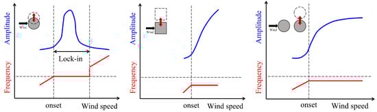
Figure 1.
Comparison of amplitude-velocity and frequency-velocity of FIV phenomenon: VIV (left); instability like galloping and flutter (middle); and, wake galloping (right).
The dynamical characteristics of lock-in makes VIV an ideal choice for fluid energy harvesting. More specifically, a VIV-based energy converter exhibits a better power performance and a higher energy efficiency when the incoming (incident) wind speed lies in the synchronization range [7].
2.2. Buffeting
Buffeting is also a resonance-type response, but the resonance results from a fluctuating incoming (incident) flow rather than from a vortex-related instability as in the “lock-in” phenomenon. As an example, the fluctuations in the incident flow can arise from the natural atmospheric turbulence as is commonly observed in long-span bridges [12] or from the oscillating wake generated by structures upstream of a bluff body as in multi-body system—this phenomenon is also referred to as wake galloping [10] (cf. right panel of Figure 1). Investigations undertaken with regard to bridge structures and aeronautics have shown that a buffeting response may occur even at low wind speeds, accompanied by a smaller oscillation amplitude and a wider frequency range than that obtained from VIV [10].
These characteristics suggest that buffeting can be utilized to harness fluid energy in a multi-body design and the power performance from such a design is expected be strongly dependent on the precise layout (arrangement) of the various oscillating bodies.
2.3. Galloping
As a representative instability response, a body subjected to galloping will first undergo a very small oscillatory motion induced by an initial perturbation. These motions result subsequently in significant oscillations once a critical incident flow velocity is exceeded (cf. middle panel of Figure 1). Galloping can occur in the transverse direction for an elastically-mounted body or in torsion for an hinged body. Torsional galloping is a much more complex phenomenon in terms of the angle of attack, the angular displacement and velocity, the phase difference and other complex dynamics involving rotational motion. It is noted that torsional galloping is not as common as transverse galloping in the context of actual engineering applications [13]. In consequence, only transverse galloping will be discussed in this paper—for simplicity, transverse galloping will be referred to as galloping hereafter.
After the onset of galloping, the vibration amplitude will increase monotonically with the increasing flow velocity and will not come to rest again even at very large flow velocities. This is the most distinct difference between instability and resonance. Galloping is associated with a much lower vibration frequency than that of vortex shedding. The characteristics of a monotonically increasing amplitude with increasing flow velocity amplitude and a frequency that is not determined by any form of lock-in is what fundamentally distinguishes a galloping (or instability) phenomenon from a resonance (VIV) phenomenon.
In general, galloping is considered to have a greater energy potential in terms of energy harvesting than VIV owing to its much larger vibration amplitudes and extended range of wind speeds for which galloping occurs, once the critical velocity for onset is exceeded. Moreover, galloping occurs only for cylinders with specific cross-sectional shapes (e.g., square, rectangular, D-section) or for cylinder–appendage systems (e.g., cylinder with an attached splitter plate)—indeed, galloping does not occur for flow past a circular cylinder. As a consequence, an energy converter utilizing galloping will require a special geometrical design in order to allow the occurrence of galloping or of the interaction of VIV and galloping.
2.4. Flutter
Flutter is also a typical non-self-limited and self-sustained fluid instability usually applicable to dynamical systems involving two or more degree of freedoms. This phenomenon is closely related to the coupling of resonant bending and torsion deformation of a body, and has some common features with galloping.
Figure 1 compares the oscillation characteristics of VIV, galloping, flutter, and wake galloping in terms of the amplitude and frequency response. As shown, all of these oscillatory phenomena have a threshold flow speed for onset—the wind speed for VIV onset is lower than that for galloping and flutter. Only VIV exhibits a lock-in of frequency and a limited displacement—the other forms of flow-induced vibration are non-self-limiting with respect to the oscillation amplitude and are associated with a frequency lower than the natural structural frequency. As discussed previously, FIV exhibits a complex taxonomy—each category in the classification corresponds to a different generating mechanism and is associated with different response modes. Furthermore, the vibration of a given bluff body can exhibit a number of different resonances and/or instabilities [1].
3. Mathematical Modelling of FIV
Mathematical modelling of FIV involves the formulation of set of ordinary differential equations (ODEs) that describe the complex physical processes associated with this phenomenon. This set of ODEs is solved numerically when given appropriate initial and boundary conditions. The success of this modelling approach depends critically on an accurate and deep intuitive understanding of the physics underlying FIV phenomena. This is the key to formulating a good theoretical model that meets the following conditions [11]: (i) simplicity of formulation; (ii) inclusion of all essential (important) characteristics of the underlying physical phenomena; (iii) utilization of concepts and quantities of interest that are physically meaningful (interpretable and explainable); (iv) capability to provide accurate and universal predictions; (v) wide applicability especially to complex cases; and (vi) possibility for model to be further developed and generalized. It should be noted that frequently the terminology of mathematical modelling as it relates to FIV concerns the theoretical analysis of the phenomenon and, in this context, it is also referred as a theoretical or analytical model. Generally speaking, a mathematical model of FIV cannot be directly derived from first principles but needs to be supplemented with various semi-empirical relationships that are obtained from experimental investigations. From this perspective, a mathematical model for FIV can also be referred to as a semi-empirical or a phenomenological model.
3.1. Classification
Presently, there are two common methods used to classify mathematical models of FIV. One was proposed by Gabbai and Benaroya [14] and involves the following three classes of models: namely, a wake oscillator model, a single-degree-of-freedom (SDOF) model and a force decomposition model. The other classification scheme was proposed by Paidoussis et al. [15]—the scheme involves also three classes of models: namely, a forced system model, a fluid–elastic system model and a coupled system model. Based on this background, we present a new formalism for the classification of FIV models that we believe makes the ordering of FIV models more legible to researchers and practitioners and makes discussing new research directions easier. From the perspective of a bidirectional FSI problem, a structural oscillation can be modelled in terms of the motion displacement using a mass–spring–damper system. However, there are a number of different strategies that can be used the model the dynamics of the fluid (in the fluid–structure interaction). Depending on the modelling methodology used for the fluid and for the coupling between the fluid and the structure, mathematical models of FIV can be classified unambiguously into two main classes: namely, a coupled wake-oscillator model and a single degree-of-freedom model as exhibited in Figure 2.
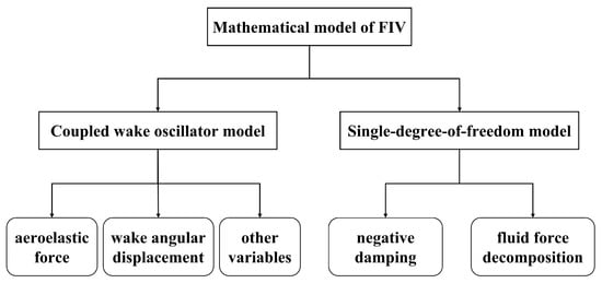
Figure 2.
Proposed classification of mathematical modelling of FIV used to predict the flow-induced vibration of a bluff body.
The coupled wake-oscillator model involves the development of a fully non-linear wake model (also referred to as a wake- or fluid-oscillator model) using either a Rayleigh-type [16] or a van der Pol-type [17] oscillator. The model includes a negative damping term in order to represent the excitation of self-sustained oscillations that are characteristic of FIV. This model is then coupled to a structure equation through a forcing term that is dependent on the state of motion of the oscillatory system. As a consequence, the coupled wake-oscillator model is composed of two ordinary differential equations whose solution can be obtained either analytically or numerically in order to predict the FIV response. In contrast to the more intuitive representation of the structural motion using the readily interpretable concepts of displacement, velocity or acceleration of a moving body, the wake-oscillator model is more abstract in the sense that it is characterized by state variables that are more difficult to interpret. Finally, we note that the interactions between the various components of the coupled wake-oscillator model involve the following processes—the aerodynamic force acts on the structure whose motion determines the angular displacement of near-wake field generated by the structure, as well as other dynamical state variables describing the dynamics of the wake.
As the name implies, the single-degree-of-freedom model consists of only one ordinary differential equation with a forcing term that is used to describe the dynamic behavior of the structure. This model is applied primarily to predict the amplitude of the FIV response [18]. The basic strategy that underpins the SDOF model is the decomposition of the hydrodynamic force (viz., the forcing term) as well as the phenomenological representation of all the force components—the self-excited response is induced on the structure by these external forces. In accordance to the nature of the forcing term, the SDOF model can be divided into two sub-classes: namely, one that is based on a mathematical formulation of negative damping and another that is based on force data obtained from experiments.
The mathematical models of FIV mentioned above will be described in detail in Section 3.2 and Section 3.3 in relation to their modelling of various FIV phenomena—VIV, galloping, and combined VIV-galloping.
3.2. Vortex-Induced Vibration
3.2.1. Coupled Wake-Oscillator Model
- (1)
- Aerodynamic force coefficient.
All the available coupled wake-oscillator models that use a physical quantity related to the aerodynamic force as the fluid variable is a derivative of the seminal ideas of Bishop and Hassan [19]. These investigators were the first to advocate using a fluctuating lift force acting on a circular cylinder to model the dynamic behavior of the near-wake region. Figure 3 displays a schematization of this kind of model—here, the instantaneous displacement of the cylinder is and the wake dynamics are characterized by a specific physical quantity (e.g., oscillating fluid force ). Following on from this effort, Hartlen and Currie [20] formulated a widely used Rayleigh-type wake oscillator in terms of the fluctuating lift coefficient and coupled this model with a damped linear system through the cylinder velocity in order to predict the transverse VIV of an elastically-mounted rigid circular cylinder. The dimensionless governing equations for this model are given by
where the dot over a quantity refers to the derivative with respect to the dimensionless time ; , , and are the normalized transverse displacement, velocity, and acceleration, respectively; is the ratio of the vortex-shedding frequency to the natural structural frequency ; is the structural mass ratio where and D are the cylinder mass per unit length and cylinder diameter, respectively; is the Strouhal number; is the fluid density; the structural damping ratio is defined as the ratio of the structural damping coefficient to critical damping; is lift coefficient for the stationary cylinder; and and b are constant coefficients that define the model.
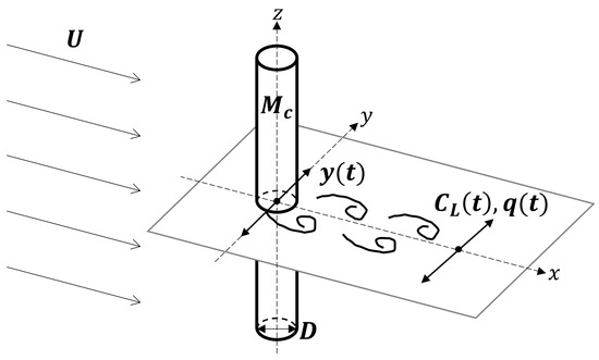
Figure 3.
A schematic model of an elastically mounted circular cylinder undergoing cross-flow VIV due to aerodynamic fluid forces acting on the oscillating body.
A number of models (both variants and generalizations) have been formulated based on the Hartlen–Currie model [20]. Skop and Griffin [21] and Griffin et al. [22] applied a modified van der Pol-type wake oscillator with concomitant model parameters describing structural properties, such mass and damping ratio and showed that the model agreed very well with experimental data. Landl [23] reformulated the Hartlen–Currie wake oscillator using a van der Pol-type oscillator and introduced a fifth-order non-linear damping term (viz., where is a model parameter) into the model in order to account the hysteresis effect of VIV. It is noted that these model variants were developed to predict the VIV of a rigid bluff body. Skop and Griffin [24] extended their earlier model [21] to predict the VIV arising from a flexible circular cylinder (e.g., a slender cable). This was accomplished by expressing the sectional vibration displacement and lift coefficient using a modal expansion (normal mode) and formulating the governing equations for the various terms in this expansion. Following on from this effort, Skop and Balasubramanian [25] introduced a so-called stall component (viz., where is a model parameter) as part of the forcing term in the structure equation. To this purpose, the transverse fluid force consists of two components: namely, one component (modelled using a van der Pol wake oscillator) that is used to cause the body to move and another component (which proportional to the negative structural velocity) which is used to reduce the amplitude of the lift coefficient for large (significant) structural motion (stall term). This innovative modification of the lift force is significant because it confers on the model the capability to predict the asymptotic VIV response in the vicinity of zero structural damping—this has, up until then, never been realized. Skop and Luo [26] further refined the stall term (viz., ) in order to ensure the accuracy of induced asymptotic behavior.
The models described above (whether for a rigid or flexible body) have the following common characteristic: namely, the wake variable is explicitly expressed in terms of the fluctuating (instantaneous) lift coefficient . Facchinetti et al. [27] first introduced a generalized dimensionless wake variable q in order to characterize the oscillating wake (cf. Equations (3) and (4)). Although in their case the action of the fluid on the structure was still considered as a lift force with q representing the reduced vortex lift coefficient ( where is the finite amplitude of a stable quasi-harmonic oscillation), Facchinetti et al. [27] demonstrated that q can be chosen to be other physical quantities that are capable of describing the fluctuation characteristics of the near wake. The dimensionless governing equations for this model can be expressed as follows:
The dimensionless quantities in this model have different definitions than those of the Hartlen–Currie model [20]. These include the dimensionless time , the structural mass ratio with M being the sum of the cylinder mass and added mass , and the frequency ratio which is now defined as . Finally, and A are constant coefficients that define the model.
Another contribution arising from the model proposed by Facchinetti et al. [27] and inspired by the effort of Skop and Balasubramanian [25] for a flexible body was the inclusion of the stall term (i.e., a fluid-added damping term) in the structure equation of motion using a drag coefficient —as a reminder to the reader, this term is given by . These investigators also examined different forcing terms for the wake oscillator (displacement, velocity, and acceleration) and found that the use of the acceleration provided the best conformance with the experimental data. The model formulated by Facchinetti et al. [27] is so popular that many variants of this model have been used in subsequent theoretical studies. For example, Ogink and Metrikine [28] introduced an acceleration–velocity coupling term () that is dependent on the oscillation frequency of the cylinder in order to provide good predictions for both forced and free vibrations.
It should be noted that all the models described above are designed to predict the one-degree-of-freedom (1DOF) transverse VIV motion of a bluff body. To be more realistic, some theoretical studies focus on modelling both the in-line and cross-flow vibrations. A number of two-degree-of-freedom (2DOF) phenomenological models have been developed based on using two governing equations for the x- and y- directions of motion in order to simulate the possible coupling between these directions of oscillatory motion. In comparison to the 1DOF models, the 2DOF models for VIV are still rather limited and will not described in detail in this paper. Interested readers are referred [29,30,31,32,33] for more information concerning 2DOF models.
- (2)
- Wake angular displacement.
Rather than representing the dynamic wake using an instantaneous lift force coefficient, Birkhoff [34] developed a linear wake oscillator based on the concept of a wake rotation angle () in order to simulate the oscillations in the near wake region behind a stationary cylinder (see Figure 4a). This model assumes the following mathematical form:
where and h are half-length and width of the near-wake lamina which can be determined using experimental data. It is noteworthy that Birkhoff’s wake oscillator is derived using physically-based concepts, such as the Kutta–Joukowsky lift theory [35,36] and Newton’s second law of motion. In this sense, Birhoff’s wake oscillator model is more of a physics-based model than models that directly incorporate a van der Pol-type governing equation.
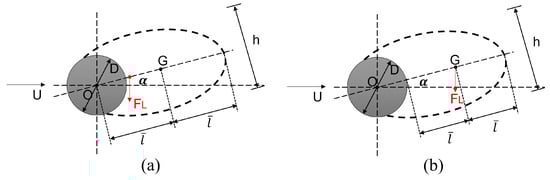
Figure 4.
A schematic of the wake oscillator model developed by (a) Birkhoff [34] and (b) Funakawa [37].
Funakawa [37] modified Birkhoff’s wake oscillator slightly based on experimental data in the following two aspects: (i) the near wake develops from the rear (back) of cylinder rather than from the cylinder center; and (ii) the location of the restoring force coincides with the center of gravity as shown in Figure 4b. With these modifications, the governing equation is given by
Tamura [38] further assumed that the wake angular displacement and wake length are dependent on the time t and replaced the constant wake length in Funakawa’s wake oscillator with time-dependent wake length. The time dependence of and were obtained from measurements of the wake dynamics behind a fixed cylinder. Furthermore, Tamura included a viscous force using a negative damping term into the ordinary differential equation and derived the associated damping coefficient using the assumption that the work done by the lift and viscous forces is equal. With these modifications, the governing equation for Tamura’s wake oscillator is expressed as
where denotes the damping coefficient of the near wake and is the Magnus factor which has a value of 1.16 for a circular cylinder [38]. We note that Equation (7) reduces essentially to a non-linear and self-excited van der Pol-type equation and, as a consequence, it can potentially be coupled to a structural equation to predict self-sustained FIV phenomena just like the lift oscillator described above. The consistency in the structure of the lift oscillator and the wake-angle oscillator suggests that the van der Pol equation provides a reasonable and effective paradigm for modelling the wake dynamics behind a bluff body experiencing FIV.
Tamura and Matsui [39] extended Tamura’s non-linear wake oscillator for a stationary cylinder to a vibrating system by coupling it to a linear mass–spring–damper system. The external driving force in the structure equation is obtained from the transverse component of the lift and drag forces, so . The forcing term of the wake oscillator is a linear function of the velocity and acceleration of the oscillation. The dimensionless governing equations for this model are given by
The quantities in these governing equations basically follow the nomenclature for the Hartlen–Currie model [20], except that mass ratio per unit length is redefined as , a damping ratio of oscillating wake is included, and the normalized wake length is defined as . The characteristic wake variable is related to the lift coefficient through the Magnus effect, so . An obvious difference between the Tamura–Matsui model [39] (which uses the angular displacement in the wake oscillator) and previous models (which use the lift (either or q) in wake oscillator) is that all the parameters in the former model have a clear physical meaning (interpretation) and can be determined from direct measurements in wind-tunnel experiments, while the latter set of models includes a number non-physical (tuning) constants (e.g., and b in Equation (2) or and A in Equation (4)) that can only be determined from curve fitting of experimental data. The reason for this is that the Tamura–Matsui model [39] is derived from series of physically-based concepts (as noted earlier) instead of assuming a priori the applicability of a van der Pol-type oscillator. The Tamura–Matsui model [39] is designed to predict 1DOF transverse VIV for a two-dimensional (2D) rigid circular cylinder and, as a result, this model can reproduce the key non-linear characteristic of VIV for this case. Finally, Tamura and Amano [40] extended the Tamera–Matsui model to a three-dimensional circular cylinder. This was accomplished by utilizing the modal expansion method for the sectional vibration displacement of the cylinder and the angular displacement of the wake.
In addition to predicting the VIV for 2D and 3D circular cylinders, Tamura and his collaborators also combined the non-linear wake oscillator in terms of the angular displacement with an equation of motion for a square cylinder in order to predict galloping and VIV-galloping. This generalization of the model will be described in detail in Section 3.3 and Section 3.4. The series of models developed by Tamura and his collaborators (which spanned the period from 1979 to 1987) are representative of mathematical models that apply the rotation angle of the near wake in order to characterize the flow dynamics behind a bluff body undergoing FIV. The interested reader can refer to a comprehensive review paper by Tamura [11] for a broad overview of the motivation, development, and derivation of these types of model.
- (3)
- Other wake variables.
Among the theoretical models that use wake variables other than the lift coefficient and the wake angular displacement, the most representative one is that proposed by Iwan and Blevins [41]. This particular model is derived from the basic fluid mechanics underpinning the von Kármán vortex street behind a cylinder (momentum equation in y-direction) and involves the introduction of a hidden fluid variable z denoting the weighted average of the transverse flow motion (e.g., velocity, acceleration) in order to formulate the vertical momentum in a control volume. Interestingly, the Iwan–Blevins wake oscillator (which is based on the physics of the flow field) also assumes the form of a van der Pol equation which, in turn, provides further support for the use of the latter model from a purely physics-based perspective.
Another interesting coupled model was proposed by Krenk and Nielsen [42], who utilized a generalized fluid oscillation displacement w of the equivalent fluid mass as the state variable in a wake oscillator. The non-linear negative damping incorporated in this model was defined as the quadratic form
where denotes the circular frequency of vortex shedding and is the vibration amplitude of fluid oscillator over a stationary cylinder. In consequence, the wake oscillator defined by this model is actually a combination of a van der Pol and Rayleigh oscillator.
3.2.2. Single-Degree-of-Freedom Model
The key to the formulation of a SDOF model is to correctly represent the forcing term so that it can induce finite-amplitude vibrations on the bluff body. A forcing term based on a negative damping is generally expressed as a forcing function F, for which the aeroelastic damping term may be offset by positive mechanical damping and causes the total system damping to be zero for a certain range of inflow (incident) wind speeds. This is the reason why the energy of the fluid is transferred from the wake flow to the bluff body, initiating the oscillation of the body. Concerning the mathematical formulation, F is a function of the status of the body motion (e.g., displacement, velocity, acceleration, oscillation frequency) and can be regarded as a “stack” of multiple vibration sources each multiplied by a corresponding prefactor that is dependent on the reduced frequency defined as (U is the inflow wind speed).
Motivated by an earlier linear model [43] as the basis for development, a representative non-linear SDOF model was proposed by Simiu and Scanlan [44]. This model is given by
In this model, the hydrodynamic force that drives VIV on the structure depends on two components. The first component is the motion-induced force that is expressed in terms of y and , which is characterized by the following non-linear damping term:
The second component is a linear stiffness term where , , and are model parameters. The combination of these two terms, especially the inclusion of van der Pol-type negative damping with a non-constant coefficient, induces the self-excited and self-limited VIV response. The other force component in the model is the vortex-shedding force that is directly related to the lift coefficient —a term which forces the structure to vibrate at the vortex-shedding circular frequency .
Ehsan et al. [45] further extended the Simiu–Scanlan model [44] for a rigid body to a long-span flexible bridge. Inspired by the coupled wake-oscillator model proposed by Billah [46], Goswami et al. [47] modified this model by replacing the direct forcing term which is dependent on in Simiu–Scanlan model with a parametric stiffness term given by . Here, is a model parameter that excites the body to oscillate at the frequency . This model can reproduce the non-linear characteristics of VIV, such as lock-in and hysteresis.
Another type of SDOF model decomposes the fluid force according to its phase difference relative to the motion of the structure. More specifically, the fluid inertial force is in-phase with the acceleration, while the fluid damping force inducing the transfer of energy from the fluid to the body (giving rise to structural oscillation) is in-phase with the velocity and displacement. Rather than deriving a specific mathematical relationship, the composed forces are obtained directly from measurements obtained from forced-vibration experiments in which the lift force is measured at a given frequency. As a result, this type of SDOF model is more suitable for the calculation of the vibration at a single distinct frequency and can be used to obtain accurate predictions of maximum response. Interested readers are referred to references [48,49,50,51] for more details regarding the development of SDOF models based on fluid force measurements.
As an example of the application of the mathematical models described in this section, Figure 5 shows the predictions obtained from three mathematical models of the normalized maximum oscillation amplitude as a function of the reduced velocity for a VIV system consisting of the flow past a circular cylinder of diameter D. The three mathematical models are those proposed by Iwan and Blevins [41] (I&B), Tamura and Matsui [39] (T&M) and Facchinetti et al. [27]. These model predictions are compared to some experimental data reported by Feng [52] for VIV of a circular cylinder with a mass ratio of 0.00257 and damping ratio of 0.00181. As shown, model proposed by Iwan and Blevins (which is based on a hidden flow variable) predicts a quite narrow lock-in and a slightly larger amplitude. The model proposed by Tamura and Matsui (which is based on the wake inclination angle) generally provides a good agreement with experimental data, although the model provides a premature termination of the synchronization. Finally, Facchinetti et al.’s model with regard to the lift coefficient gives a reasonably accurate prediction of the lock-in range, but the onset of VIV occurs at a smaller value of . It should be noted that the mathematical model predictions depend critically on the appropriate selection of the parameters for each model, and the values of these parameters can vary from case to case.
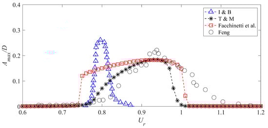
Figure 5.
Comparison of predictions of the maximum oscillation amplitude as a function of the reduced velocity of the VIV of a circular cylinder with diameter D obtained using three mathematical models with a benchmark experiment conducted by Feng [52], Iwan and Blevins [41] (I&B), Tamura and Matsui [39] (T&M) and Facchinetti et al. [27].
3.3. Galloping
Galloping is an important aeroelastic response of a bluff body—its analytical modelling is generally based on the so-called quasi-steady (QS) hypothesis which states that the instantaneous aeroelastic force exerted by the fluid on a vibrating structure is the same as that on a stationary body at the same angle of attack.
Figure 6 displays the simplest physical model for the analysis of the galloping behavior of a cylindrical body restrained to oscillate only in the transverse direction and subjected to an uniform streamwise inflow (incident) wind speed of U [53]. As shown, the damped spring-mounted system is characterized by the mass per unit length , the mechanical damping coefficient , the spring stiffness k, and the characteristic length D of the body normal to incoming flow. The structural motion is governed by the following dimensional second-order ordinary differential equation:
where is the lateral aerodynamic force inducing the galloping which can be calculated using QS theory. Once the body begins to move in the transverse y-direction (viz., ), the relative velocity between the oscillating body and the fluid is and the angle of attack (AOA) is determined using which varies periodically over time owing to the transverse oscillation of the structure. The time variation of the AOA induces a time variation in the lift and drag forces given by and . The lift and drag coefficients can be determined from conducting static experiments.
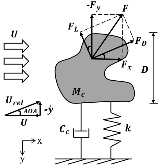
Figure 6.
Schematic of a bluff body experiencing transverse galloping in a fluid flow.
The transverse fluid force is a function of AOA and will vary with time. This force component can be derived by projecting the lift and drag forces and along transverse y-axis [2]:
The force component can also be formulated in terms of the transverse force coefficient as follows:
It should be noted that the velocity in Equation (15) is the inflow (incident) velocity U (rather than ) which is referenced to a direction perpendicular to the direction used to define . Equations (13)–(15) can be combined to obtain the transverse force coefficient given by
To model the incipient instability at the onset to galloping (viz., implying that ), one can apply a one-dimensional Taylor series expansion for about the point . The Taylor series expansion of truncated at the first-order term is given by
The second term on the right-hand side can be treated as the contribution to the effective system damping (also called fluid dynamic damping) [9] arising from the aerodynamic forces. This term can be merged with the mechanical damping term (second term on the left-hand-side), so that the total damping ratio assumes the following form:
The prerequisite for galloping is the presence of a negative system damping (viz., ). Because the mechanical damping is positive (), the second term on the right-hand-side of Equation (19) is less than zero, so
Equation (20) is the well-known Glauert–den Hartog galloping criterion [54] setting the necessary condition for aerodynamically unstable behavior of a SDOF oscillator. This criterion can also be used to evaluate the galloping onset by setting the mechanical damping to be equal to the fluid dynamic damping giving
The rationale underlying the Glauert–den Hartog galloping criterion is related to the boundary-layer separation and reattachment phenomenon at a certain angle of attack [55,56,57].
Parkinson and Brooks [58] combined the aerodynamic force derived from QS theory with a linear dynamical system to develop a non-linear self-excited oscillation model for a bluff body experiencing 1DOF “plunging” oscillation (viz., galloping). The variation of the aerodynamic force coefficient in the transverse direction () as a function of AOA (obtained from static test data of the lift and drag coefficients ( and ) for different angles of attack) was fitted with a fifth-order polynomial. This polynomial approximation for as a function of AOA was then incorporated as a forcing term in the governing equation for a linear mass–spring–damper system. Subsequently, a more accurate seventh-order polynomial fitting of (see Equation (22)) was used in order to reproduce hysteresis effects observed in wind-tunnel experiments [59]. The seventh-order polynomial approximation for has the following form:
where , , , and are fitting coefficients for the model. The corresponding dimensionless equation of motion for a square cylinder can be written as follows:
where is the reduced velocity. The Parkinson–Brooks model [58] can be solved analytically using various approximation methods when the mass ratio is small (e.g., in air is typically of order ). As an example of this strategy, Parkinson and Brooks [58] used the Krylov–Bogoliubov asymptotic method to solve Equation (23) and found that the (approximate) solution provided a good agreement with some wind-tunnel measurements. Furthermore, Equation (23) can be solved numerically (using, for example, the fourth-order Runge–Kutta method). The form of Equation (23) resembles the SDOF model for VIV, described previously in Section 3.2.2, in the sense of having one governing equation where the forcing term is related to the aerodynamic force acting on structure—the only difference between these two models is that the force coefficient used to model galloping involves a polynomial that has been fitted to experimental data of the static force as a function of the angle of attack.
The result provided by the QS model is highly dependent on the polynomial fitting . Luo et al. [60] and Ng et al. [61] compared different high-order polynomials and found the minimal order of the fitting polynomial needs to be seven in order to capture the key characteristics of as a function of AOA and to predict certain features of the non-linear dynamics of galloping, such as hysteresis. Using a ninth- or eleventh-order polynomial may provide a better fit to the variation of with AOA, but this does not change the characteristics of the governing equation, such as the number of positive real roots representing the stationary oscillation amplitude of a bluff body, implying that the predicted galloping hysteresis would be the same as that obtained from a seventh-order polynomial approximation for . Barrero-Gil et al. [62] and Joly et al. [63] also incorporated the Reynolds number () into the classical QS galloping model by expressing the polynomial coefficients as a function of in order to investigate the occurrence of galloping and the hysteresis effect of a square cylinder in the laminar flow regime.
From a physical and mathematical viewpoint, the underlying QS assumption is that the transverse galloping force depends on the instantaneous position of the body, as well as on the instantaneous relative velocity between the body and the fluid [64]—this is true in certain circumstances, such as when vortex shedding frequency is much larger than the structural oscillation frequency (viz., ), implying that the wake dynamics are essentially uncoupled from the body motion so that the influence of the vortex force on the galloping driving force is negligible. In addition, the applicable velocity range of the QS model is determined (approximately or better) by the condition where the Strouhal number often has an order of magnitude of 0.1, suggesting that the QS assumption can be satisfied at large values of [62,64,65,66]. Even with these limitations, the easy-to-use QS model still plays a fundamental role in the mathematical modelling of galloping, especially when few experimental or numerical data are available.
The den Hartog criterion and QS galloping models are limited to 1DOF translational galloping. There also exists some QS-based theoretical models for 2DOF galloping (vertical and torsional) [13,67,68] or for 3DOF galloping (vertical, lateral, and torsional) [64,69,70].
3.4. Combined VIV and Galloping
Instead of undergoing VIV or galloping only, some engineering structures with aerodynamically unstable cross-sectional shapes can experience the mutual effect of both types of FIV phenomena. Parkinson and Sullivan [53] and Parkinson and Wawzonek [71] conducted some wind-tunnel experiments involving square and rectangular towers, which demonstrated that the synergy between VIV and galloping can provoke large-amplitude transverse vibrations that are not predicted using models for either galloping or VIV. As a consequence, it is of practical importance to construct a simple and efficient mathematical model for a (combined) VIV-galloping response. Based on the discussion in Section 3.2 and Section 3.3, the essential problem still reduces to correct simulation of the unsteady aerodynamic force responsible for the dynamic response—the most straightforward way to accomplish this is to simply superimpose the VIV and galloping force components.
An early theoretical work following this methodology was proposed by Parkinson and Bouclin [72] who used the Hartlen–Currie lift oscillator [20] to calculate the fluctuating lift force due to vortex shedding that induces the VIV () and the Parkinson–Smith quasi-steady model [59] to represent the perturbational transverse force that triggers galloping (). In this approach, the sum of both these forces is incorporated as the forcing term in the structural equation of motion and used to predict either VIV or galloping response of a bluff body.
Corless and Parkinson [73] modified the Parkinson–Bouclin model [72] by adding an acceleration coupling term in the wake oscillator. With the inclusion of this term, the Corless–Parkinson model assumes the form
where the coefficients , and are functions of . These coefficients can be determined by curve fitting of experimental data. The other quantities in Equations (24) and (25) are consistent with those described earlier for the Hartlen–Currie lift oscillator [20] (see Equations (1) and (2)). The system of ODEs here were solved using the Multiple Time Scales (MTS) method.
Following the same strategy, Han et al. [74] incorporated the quasi-steady galloping force into another representative lift-type wake-oscillator model—Facchinetti et al.’s model [27]—to give a coupled mathematical model for VIV-galloping of a square prism. Using the same dimensionless terms as in the model proposed by Facchinetti et al. [27], the formulation that incorporates acceleration coupling and a seventh-order polynomial fitting of the galloping force reduces to the following form:
It is possible to combine not only the lift oscillator model with the QS model for galloping, but also the wake oscillator model with the wake rotation angle as the state variable (see Section 3.2.1). Tamura and Shimada [75] proposed a mathematical model for the interaction of the VIV resonance with galloping for 2D and 3D rigid square cylinders. In this model, the unsteady vortex shedding and galloping forces were simulated using the Tamura–Matsui VIV model [39] and the QS model developed by Parkinson and colleagues [58,59], respectively. Following the nomenclature used earlier in Equations (8) and (9), the model recast in dimensionless form is given by
The models described above have been important mathematical tools for the prediction of combined VIV and galloping for a square cylinder. These basic models have been validated and extended in a number of ways. An important contribution in this respect is the body of work conducted by Mannini and colleagues [76,77,78,79]. In particular, Mannini et al. [76] compared the Corless–Parkinson model [73] and the Tamura–Shimada model [75] for the prediction of the FIV response of a rectangular cylinder and validated their model performance using their wind-tunnel test data. A key conclusion of this investigation was that the Tamura–Shimada model [75] is more accurate than the Corless–Parkinson model [73] in terms of their predictions of the correlation between the oscillation amplitude and the wind speed over the range where galloping occurs. Furthermore, Mannini et al. [77] modified the Tamura–Shimada model [75] by replacing Funakawa’s wake oscillator [80] (see Figure 4b) with Birkchoff’s wake oscillator [34] (see Figure 4a) and used an improved tuning process of the model parameters. These investigators also incorporated the effects of turbulence into the modified the Tamura–Shimada model [78]. Finally, Chen et al. [79] proposed a more reasonable definition of the near-wake laminar for a rectangular cylinder—the modified model was shown to provide better predictions of the (combined) VIV-galloping instability.
4. Numerical Modelling
Owing to the continuous advancement of computational fluid dynamics (CFD) and computer-aided engineering (CAE) in recent years, numerical modelling of the complicated FSI problems such as the FIV of a bluff body is now practical for real-world engineering and industrial problems. The various forms of CFD that can be used to model numerically the FIV of a bluff body include direct numerical simulation (DNS), large-eddy simulation (LES), detached-eddy simulation (DES), delayed detached-eddy simulation (DDES), and Reynolds-averaged Navier–Stokes (RANS) modelling, among others. The numerical discretization approaches used to solve the fluid dynamics equations for these various approaches encompass the finite-element method (FEM), the finite-volume method (FVM), the finite-differencing method (FDM), spectral elements method (SEM) which is essentially a Galerkin-based FEM with Lagrange shape functions, the discrete vortex method (DVM), the entropy–viscosity method (EVM), the lattice-Boltzmann method (LBM), among others. The fluid–structure interaction schemes include either a moving-mesh or a fixed-mesh strategy. The commonly-used numerical codes for addressing FIV of a bluff body include the various commercial programs, such as Ansys Fluent [81] (which uses FEM) from Ansys Inc. and STAR-CCM+ [82] from Siemens PLM, as well as open-source software packages, such as OpenFOAM [83] (which uses FVM and unstructured grids).
For the benefit of those readers who are unfamiliar with CFD—the key-enabling technology underpinning the numerical simulation of FIV phenomena—we will provide a brief overview of the key concepts. The basic idea of CFD is to use appropriate algorithms to solve some form of the Navier–Stokes (NS) equations that describe the fluid flow. To this purpose, the NS equations that govern a viscous, incompressible flow, whether laminar or turbulent, express the conservation of mass (incompressibility of the fluid volume) and the conservation of momentum, respectively, as follows:
and
where is the Cartesian coordinate associated the i-th direction (so, ); is the Cartesian fluid velocity component in the direction; p is the pressure; is the fluid density; is the fluid kinematic viscosity; and, t is time. In the above equations, the Einstein summation convention is assumed to apply to repeated indices.
In direct numerical simulation (DNS), the NS equations is solved numerically with the entire band of scales of the flow from the large energy-producing to the small dissipative motions fully resolved in space and time. Here, no ad hoc models are required to represent the unresolved motions of the flow. The application of DNS is currently restricted to low and moderate Reynolds numbers (laminar or weakly turbulent flows). For larger Reynolds number flows (strongly turbulent flows which are prevalent in engineering and geophysical applications), a simpler level of description is required. To this purpose, one can apply a filtering (averaging) operation to the NS equations. The resulting filtered (averaged) NS equations give rise to more unknowns than the number of equations—unknown subgrid stresses or Reynolds stresses in the momentum transport equation—resulting in the so-called turbulence closure problem. In large-eddy simulations (LESs), only the large-scale portion of the turbulence is explicitly computed while the small-scale portion (subgrid scale or SGS) of the fluid motions are represented using a so-called SGS model. Alternatively, in the statistical simulation of the fluid flow based on the Reynolds-averaged NS (RANS) equation, the averaged effect of the turbulence on the flow (embodied in the Reynolds stress tensor) is modelled. Finally, there are hybrid methods of fluid flow simulation (e.g., detached-eddy simulation or DES) in which a RANS model is used to represent some parts of the flow (e.g., near solid walls) while LES (with a SGS model) is used elsewhere, hence providing a compromise between the computational expense of LES and the computational efficiency of RANS. For more information on CFD, the reader is referred to [84].
The numerical modelling of FIV is capable of providing accurate predictions, as well as deeper physical insights into the fundamental processes underpinning the FIV response. In consequence, numerical simulations are a invaluable tool that complements physical experiments for the practical design and analysis of a bluff body subjected to FIV. Even so, we stress that the FIV problem involves very complex flow dynamics and non-linear bidirectional interactions between the fluid and the structure—these complexities limit the predictive capabilities of FIV simulations, especially in the high-Reynolds number (and strongly turbulent) flows in the range of from to . It should be stressed that real-world FIV problems almost always involve flows in this flow regime where either the three-dimensional flow transitions from laminar to turbulent or the flow is fully turbulent [85]. These limitations prevent CFD being used exclusively to address real-world engineering and industrial problems involving FIV phenomena. Nevertheless, it can be stated that improvements of accuracy and reliability of FIV numerical simulations for flows in the subcritical and high-Reynolds number range is essential in order to provide confidence in the use of numerical modelling of FIV for addressing real-world applications.
4.1. Numerical Techniques for FSI Simulation
The numerical simulation of a two-way FSI problem, such as FIV involves both the effect of the fluid flow on the motion of the structure and, conversely, the effect of the structure on the local flow. As shown in Section 3, the precise mathematical description of FIV consists of the governing equations for the fluid flow dynamics (NS equations) which are then coupled to the equation of motion for the structure (which generally is modelled as a mass–spring–damper system). This coupled set of equations needs to be solved numerically. The use of an appropriate fluid–structure interaction strategy is critical for the simulation of the coupled dynamics of the fluid–structure interaction. Depending on the treatment of the computational mesh, the numerical methodologies for the simulation of FSI can be stratified into two categories: namely, a moving mesh (or conforming) method and a fixed mesh (or non-conforming) method [86].
- (1)
- Moving mesh.
The moving mesh method involves a dynamic re-meshing (or mesh updating) of the computational grid at each time step (viz., the mesh moves to accommodate the dynamically changing topology of the spatial fluid domain owing to the motion of the structure which, in turn, necessitates the tracking of the fluid–structure interface at each time step). As a consequence, an efficient moving mesh module and a fast and automatic mesh deformation procedure are of great importance for the successful simulation of a FSI using this approach.
An often-used mesh diffusion scheme is exhibited in Figure 7. In this scheme, the mesh around the moving body (green) moves with the body without any deformation as if the mesh was “rigid” (viz., attached to the body). The outer boundary cells (white) in this scheme remain fixed—only the portion of the computational grid lying between the inner and outer boundaries (orange) are deformed and re-generated at each time step. This moving mesh scheme has been demonstrated to give almost no projection error in the solution and, furthermore, improves the accuracy of the simulations by preserving the gradients in the vicinity of the moving body [87,88]. Another key issue is the mesh morphing algorithm that deals with the motion of the body. As an example, the displacement and velocity of the mesh in the orange region of Figure 7 for each time step is obtained from the solution of a Laplacian equation. The reader is referred to Ref. [89] for more details of mesh deformation methods (remeshing or adaptive meshing strategies).
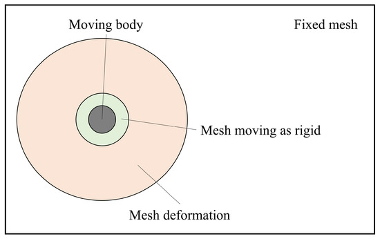
Figure 7.
Schematic describing the components of a mesh moving scheme.
A classical and popular moving mesh technique is the arbitrary Lagrangian–Eulerian (ALE) algorithm, which can both follow the moving boundary and preserve the mesh grid shape even for large structural displacements at the same time. This algorithm accomplishes this by defining three domains: namely, a material domain to provide a Lagrangian formulation of the moving body, a spatial domain described in an Eulerian (fixed) reference frame, and an arbitrary domain involving an arbitrary motion that determines the deformation of the moving mesh. The mapping of ALE to the NS equations involves explicitly incorporating an arbitrary mesh velocity into the convective term of the momentum transport equations, so that the body motion and the mesh deformations required to maintain an adequate spatial discretization can be taken into account. It should be noted that in the ALE scheme, the computational grids are allowed to move independently of the fluid velocity in order to avoid an excessive distortion of the mesh. Another common moving mesh technique is the so-called Deforming-Spatial-Domain/Stabilized Space-Time (DSD/SST) algorithm, which has been used by Mittal and Kumar [90] and by Singh and Mittal [87] in their numerical simulations of FIV.
In general, the numerical computation involved in the application of a moving mesh approach consists of three basic steps [91]: (1) the fluid dynamics computation; (2) the structure dynamics computation; and (3) the mesh movement computation. A detailed flowchart showing how these steps are implemented is displayed in Figure 8 for the ALE algorithm (left panel). For examples of the application of the ALE algorithm to address the FIV problem, the interested reader is referred to references [85,92,93,94,95,96,97]. The moving-mesh method using a body-fitted coordinate system can generally achieve a high-mesh resolution near the moving boundary and, as a result, can provide excellent simulations in that critical portion of the flow field (viz., where the fluid and the structure interact). However, this methodology requires frequent updating of the mesh (usually at every time step) which may be computationally prohibitive—hence, limiting the wider acceptance of the methodology for addressing FSI problems (particularly those involving very large amplitudes in the motion of the body giving rise to large distortions of the mesh).
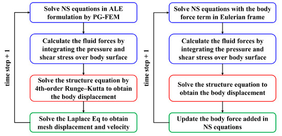
Figure 8.
Numerical computational procedure for the simulation of FIV of a bluff body using the ALE algorithm for a moving mesh scheme (left panel) and the immersed boundary method for a fixed mesh scheme (right panel).
- (2)
- Fixed mesh.
To circumvent some of the problems associated with using a moving and regenerating mesh in the body-conforming formulation, a fixed mesh method can alternatively be used for FIV simulation. This methodology uses the notion of an immersed method that employs an overlapping description of the fluid (in an Eulerian frame) and the structure (in a Lagrangian frame) and a non-conforming fluid–structure interface in order to avoid the movement of the mesh (and concomitant re-meshing) at each time step [86,98]. In this case, the fluid–structure interaction can be taken into account by including an additional inertial forcing term into the NS equations, resulting in the transformation from the dynamic Lagrangian coordinate system (for a moving body computation) to a fixed Eulerian coordinate system (for the fluid computation). Needless to say, the method used to determine the body force and how to distribute this force from the “immersed” points into the surrounding Cartesian grid will significantly affect the accuracy of the immersed method [99].
The immersed boundary method (IBM) is a popular non-conforming mesh technique that is based on a fixed Cartesian grid that is not fitted to the geometry of the moving body [100]. This methodology considers the moving structure as a moving boundary that is represented using a set of discrete Lagrangian points and resolves the fluid dynamics on a fixed Eulerian mesh. In order to couple the Eulerian and Lagrangian variables, IBM formulates the body force term (included in the momentum transport equations) as an integral representation involving Dirac delta function kernels—these are generally replaced with regularized delta function kernels in the numerical treatment. In comparison to the moving mesh scheme, IBM is advantageous in that there is no need to regenerate the computational mesh at each time step as a result of the motion of the body. This dramatically improves the computational efficiency for a complex FSI problem, especially in cases involving a changing topology. However, it should be stressed that this computational efficiency comes with a price: namely, the solution obtained using this methodology is probably less accurate in the vicinity of the fluid–structure interface. The steps involved in the application of IBM for FIV simulation are summarized in Figure 8 (right panel).
Apart from IBM, there are other fixed mesh schemes such as the fictitious domain (FD) method [101], the embedded boundary (EB) method [102,103], the immersed interface method, and the immersed body method. These methodologies are useful for the case where the geometric complexity of the fluid–structure interface is so complicated that it would be difficult to address using a moving mesh technique.
In summary, this section provides a brief review of two commonly used numerical methodologies for the simulation of FIV of a bluff body. For a more detail description of these methodologies, the interested reader is directed to references [86,98,104].
4.2. Two-Dimensional or Three-Dimensional Numerical Simulations of FIV
It is known that the FIV response of a bluff body is inherently three-dimensional at a high-Reynolds number in the turbulent flow regime. As a consequence, 2D numerical simulations of FIV for this case are not adequate to capture all the dynamical characteristics of this three-dimensional turbulent flow. Moreover, it should be stressed that even fully 3D turbulence simulation or modelling methodologies (e.g., 3D numerical simulations using LES, DES, RANS) can potentially not fully reproduce the complex flow dynamics in this case, especially for a laminar–turbulence transition that can occur in wakes, shear layers, and boundary layers [105]. In principle, the only numerical methodology that can potentially simulate every aspect of turbulence is DNS which involves solving the three-dimensional NS equations exactly. Unfortunately, a full numerical simulation must provide a complete solution for both the fluid dynamics and fluid–structure interaction which for high-Re turbulent flows is computationally, prohibitive (even insuperable using current computational technology). Nevertheless, if we are interested in the modelling (approximation) of the principal characteristics of the flow field, both the 2D and 3D numerical solutions obtained using either LES or RANS do provide a reasonably accurate approximation of the FIV response of a bluff body.
To this purpose, 3D numerical simulations should be used if the predictive accuracy of the fluid forces and structural response is required, as in a research problem. However, for addressing engineering and industrial FIV problems where parametric studies involving a large number of test cases are required, 2D numerical simulations with modest computational resources may be sufficient (indeed attractive). On the one hand, it has been demonstrated that 2D simulations of the FIV of an elastically-mounted cylinder may be sufficient owing to the fact that oscillations of the cylinder result in a significant increase in the wake correlation length—an increase which drastically diminishes the 3D effects of the vortex shedding [106]. This implies that 2D simulations can be used to provide good predictions for various integrated parameters, such as the aerodynamic forces coefficients. On the other hand, the largest discrepancy between 2D and 3D simulations is expected for high-Reynolds number flows involving strong turbulence effects which are not completely accounted for in a 2D simulation. As an example, the lift and drag coefficients obtained from 2D simulations in this case are overpredicted. Indeed, a number of features in the upper branch of the VIV amplitude response at high values of as obtained from experimental data are not present in 2D low- simulations—and, moreover, the corresponding vortex modes are different. In view of this, it is of great importance to ascertain whether a 2D simulation is sufficient to capture the relevant physical mechanisms of FIV in the problem of interest or whether it is necessary to resort to more computationally prohibitive 3D simulations [106] to address the problem.
To determine whether a 2D numerical simulation can be used to address an inherently 3D FIV problem to give useful results, it is necessary to consider firstly whether the wake structures for the problem are essentially two-dimensional (viz., it is necessary to ascertain the threshold Reynolds number for the onset of three-dimensional instabilities for the bluff body under consideration). It is well known that with increasing Reynolds number, the wake of a cylindrical body undergoes a transition from a two-dimensional flow to a three-dimensional perturbation. The critical Reynolds number at which this occurs is determined by the geometric shape and other constraints on the cylinder. A large body of research has demonstrated that the threshold Reynolds number for the flow transition to three-dimensionality over a stationary body occurs at a Reynolds number of about for a circular cylinder [107,108] and about for a square cylinder [109]. For other cross-sectional shapes, such as a rectangular cylinder, an elliptic cylinder, and a flat plate, the critical Reynolds number is a function of the aspect ratio [110,111]. If the cylinder is free to move, the value of the critical Reynolds number is generally larger than that for the stationary cylinder. For example, for a transversely oscillating circular cylinder, –300 [96,112]. Because the flow is essentially two-dimensional (approximately or better) for , it is advantageous (in terms of both accuracy and computational efficiency) to perform 2D simulations of FIV for flow Reynolds numbers less than . For these cases, it is expected that the results are reliable and effectively identical to the 3D simulations of FIV (at least for the primary dynamic responses, although some discrepancies may exist in the predictions for the vortex-shedding patterns). Another consideration concerning whether a 2D numerical simulation can be used to address a FIV problem stems from the fact that the inducing mechanism of relevant dynamics of the flow and structure, such as the branching behavior, the frequency lock-in, the phase jump and the wake mode has no direct relevance to the presence of three-dimensionality in the flow, so that a knowledge of these 2D characteristics can provide valuable information for the more complex 3D flow due to the qualitative similarities between them. To this point, Leontini et al. [112] analyzed in detail the genesis of 3D higher-Re flow behaviors present in a 2D flow in terms of the vibration amplitude, the frequency, and the phase difference.
If the above two considerations have been addressed, one efficient strategy to take full advantage of both 2D and 3D numerical simulations would be to first carry out a large number of 2D numerical simulation cases covering the whole spectrum of relevant parameters at low-Reynolds number, and then conduct a few representative 3D high- numerical simulations to investigate in detail the cases of interest from the perspective of the three-dimensional flow structures.
4.3. Direct Numerical Simulation (DNS) of FIV
4.3.1. Two-Dimensional DNS in the Laminar Regime
Owing to the prohibitive computational cost and uncertainties in turbulence modelling, most numerical simulations of FIV of a bluff body are conducted at a low-Reynolds number for laminar flow. This involves solving the two-dimensional NS equations coupled with the structure equation of motion. Indeed, a 2D DNS is an indispensable tool for exploring the physical mechanisms and obtaining a fundamental understanding of FIV phenomena.
- (1)
- Single cylinder.
Mittal and various collaborators conducted a series of seminal 2D simulations of the VIV response of a single circular cylinder at a low-Reynolds number. Mittal and Kumar [90] reported the “soft-lock-in” phenomenon (where ) in a 2DOF-VIV of a circular cylinder at a low mass ratio for —a phenomenon that appears to be related to a self-limiting mechanism of the cylinder. Using 2D DNS, Singh and Mittal [87] found that the Reynolds number (–500) has a significant influence on the VIV amplitude and vortex shedding mode. More specifically, the latter transitions from a 2S mode for to a P + S mode for . Furthermore, blockage has an important impact on the non-linearity of 2DOF-VIV-like hysteretic behavior at a low-Reynolds number [113]. Prasanth et al. [114] investigated the combined effect of mass ratio and blockage on the transverse oscillation of a circular cylinder and found that the hysteretic behavior appears when the critical mass ratio exceeds a value of 10.11. Prasanth and Mittal [115] conducted a comprehensive numerical study of 2DOF-VIV of a circular cylinder at a low-Reynolds number of –200 and discovered that a phase jump of 180 occurring in the middle of the lock-in range is related to the self-limiting mechanism of VIV. Mittal [116] conducted 2D numerical simulations for flow past a circular cylinder under a number of different conditions (e.g., increasing/decreasing , unsteady/steady flow) and reported a multi-branch VIV response of the cylinder at —these results were used to define a new branch which was referred to as Initial Branch II.
Leontini et al. [117] reported two branches in the VIV amplitude response at and suggested that a 2D low- numerical simulation can be used to garner deeper physical insights into the results obtained from a 3D high- simulation (at least as it concerns the nature of the underlying physical mechanisms responsible for important VIV response features). Ji et al. [101] demonstrated the feasibility of using the fictitious domain method for the simulation of a 2DOF-VIV of a circular cylinder at a low-Reynolds number of . These researchers focused on how the Skop–Griffin parameter (), which encapsulates the combined effect of mass and damping on the structure, determines the nature of the VIV response. Their numerical simulations showed that the response amplitude decreased rapidly with increasing values of . Li et al. [118] conducted numerical simulations at low-Reynolds number and at small mass-damping parameter in order to analyze various non-linear phenomena associated with 1DOF- and 2DOF-VIV (e.g., lock-in, beating, phase-switching, limit cycles, bifurcation) at low-Reynolds number and low mass-damping parameter. These investigators concluded that the streamwise vibrations influence the transverse vibrations. Étienne and Pelletier [119] utilized results obtained from numerical simulations of a zero mass and zero damping vibrating circular cylinder in order to define the regions in the plane where vibrations are either absent or present—these results showed that transverse vibrations occur for a reduced velocity . Bourguet and Jacono [120] performed a parametric study using 2D numerical simulations to investigate the transverse VIV of a rotating cylinder with a given rotation rate at Re = 100. These researchers reported a bell-shaped amplitude response, the maximum amplitude of which was three times that of the VIV of a non-rotating cylinder. In addition, the autorotation of the cylinder was found to affect the wake pattern, the lift frequency and the phase. Zhao et al. [121] conducted numerical simulations of the 2DOF-VIV of a rotating circular cylinder at a low rotation rate at and found that the forced rotation of the cylinder significantly enhances the in-line oscillation amplitude and lock-in range.
Some recent numerical studies of the VIV characteristics of a single circular cylinder in laminar flow include the following: VIV of a cooled circular cylinder in the presence of thermal buoyancy [122]; some unusual behavior in the time history of the displacement, frequency, and lift coefficient of VIV [123]; and the presence of a three-branch VIV response for a low mass-damping cylinder at low Re = 300 [124].
A number of researchers have conducted 2D simulations of laminar flow past elastically-mounted non-circular cylinders (e.g., elliptical, square, rectangular, triangular). A circular cylinder can be considered as a special case of an elliptic cylinder with an aspect ratio of unity. As a consequence, the effect of the aspect ratio (viz., ratio of the cylinder dimension in the transverse direction to that in the streamwise direction) on the FIV response of an elliptic cylinder can be studied numerically. For example, Yogeswaran et al. [125] systematically investigated the dynamics of a freely vibrating elliptic cylinder at eight different aspect ratios AR () in the laminar flow regime (). These researchers examined the VIV response (amplitude, phase lag, fluid force), the flow pattern in the wake, and the hysteresis phenomenon and found that the peak amplitude increases with an increasing AR. Chen et al. [126] found that the aspect ratio has a significant effect on the VIV response and on the heat transfer to the elliptical cylinder. Leontini et al. [127] investigated the FIV response of an elliptic cylinder with a fixed aspect ratio of 1.5 for various angles of attack AOA (viz., the angle between flow direction and major axis of ellipse) in the range . These researchers observed that the VIV for the elliptic cylinder is very similar to that of a circular cylinder for . However, it was found that a galloping-type oscillation may be triggered when , which may be due to an enhancement of the lift force by the stronger wake vortices.
It is well known that the flow past a square cylinder can exhibit both VIV and galloping owing to its asymmetry. Research conducted for the flow past a square cylinder has focused primarily on the specific conditions that trigger galloping, such as the critical values of the Reynolds number [128,129,130,131], the mass ratio [63,129,130,131,132], and the angle of attack [95,133]. In general, the consensus is that a light square cylinder can undergo galloping for , but exhibits VIV for and for intermediate angles of attack provided the Reynolds number exceeds some critical value. Two-dimensional simulations at low-Reynolds number can also be utilized to generate a large dataset of lift and drag coefficients which, in turn, can be used to determine the parameters of that determine a quasi-steady galloping model [63]. The FIV characteristics of a square cylinder under other conditions can also be investigated using 2D numerical simulation (e.g., shear flow past a square cylinder [134]). A rectangular cylinder is the generalization of a square cylinder having different aspect ratios (viz., an aspect ratio other than unity). Presently, low-Re 2D numerical simulations of the flow past a rectangular cylinder have focused primarily on the effect of the aspect ratio on the dynamic response of the vibrating system. For example, Zhao [97] investigated the flow past a rectangular cylinder for five different aspect ratios (namely, 0.3, 0.5, 0.7, 1, and 1.25) and observed that both VIV and galloping occur provided the aspect ratio is larger than 0.3. Similar to square and rectangular cylinders, a triangular cylinder is also prone to galloping due to the presence of sharp corners in the structure, to fixed separation points and to the afterbody in the separated wake. Wang et al. [135] investigated the streamwise and cross-flow FIV responses of a triangular cylinder under three typically low incidence angles (namely, 0, 30, and 60) at Re = 100. They found the dynamic response at the small incidence angles of 0 and 30 exhibited VIV similar to that for the flow past a circular cylinder, while for the larger incidence angle of 60 the dynamic response exhibited galloping.
- (2)
- Passive turbulence control cylinder.
Two-dimensional numerical simulations can be used to study the flow past a cylinder with passive turbulence control (PTC) which is, perhaps, the simplest flow control strategy employed to control the intensity of motion of a body. Passive turbulence control involves either attaching to or placing around the body one or more small device(s) (e.g., rod, splitter plate, roughness plate, fairing) to control the intensity of motion of the body.
Small controlling rods are one of the most commonly used PTC devices. Zhao et al. [95] used numerical simulation to investigate the dynamical characteristics of a PTC cylinder consisting of a circular cylinder of diameter D and a small rod (with diameter 0.2 D) attached at different angular locations on the cylindrical surface. Liu et al. [136] fixed the control rod upstream of a cylinder of diameter D and studied the effects of rod diameter (0.4 D, 0.6 D, and 0.8 D) and center-to-center spacing between the cylinder and rod (1.2 D and 2.8 D) on the dynamical response of the system. Liu et al. [137] used the numerical simulation of a cylinder–rod system, consisting of a cylinder of diameter D and six detached controlling rods of diameter 0.25 D in order to investigate the effect of the separation (ranging from 0.1 D–2 D) between the cylinder and the multiple rods on the dynamical response.
The splitter plate is another easy-to-use flow control device. Various configurations, such as the relative location of the splitter plate with respect to the main cylinder (e.g., upstream, downstream, side-by-side), the type of connection (e.g., attached or detached), the nature of the plate material (e.g., flexible or rigid), the constraints applied to the cylinder and/or plate (e.g., fixed or free) and the plate length can be investigated using 2D numerical simulations in laminar flow. For these various configurations, the effect of the mass ratio, of the damping ratio, of the Reynolds number, of the plate length, and of the separation between the cylinder and the detached plate can be studied [138,139,140].
- (3)
- Array of cylinders.
An array of cylinders is a more realistic and practical system to study than a single cylinder owing to the fact that this configuration is found frequently in the form of offshore platforms (floating or fixed), multiple marine risers, and a fluid energy harvester system. We consider the simpler case where each cylinder in the cylinder array has the same diameter. Needless to say, the dynamic response of a cylinder array is expected to be much more complex than that of a single cylinder—an observation which highlights the challenges that need to be confronted if such a system is to be investigated numerically using 3D flow simulation at high-Reynolds number. In view of this, it is expected that 2D low-Reynolds number numerical simulations are useful for providing the much needed physical insights into the dynamic response and the underlying physics of a multi-cylinder system.
Carmo et al. [106] applied 2D numerical simulations at Re = 150 to study the effect of the separation between two cylinders on the FIV response of the system. In this study, the separation between the two cylinders is carefully selected such that the downstream freely-vibrating cylinder experiences the transverse FIV (wake galloping) that results due to the wake shed from the upstream fixed cylinder. The numerical results show that the tandem two-cylinder system provokes FIV with a wider synchronization boundary, a larger maximum amplitude, and an overall larger vibration amplitude at high speeds in comparison with that obtained for a single cylinder. This may be due to the presence of an oscillatory flow between the two cylinders that is absent for a single cylinder. Other numerical studies have focused on a number of different configurations of the cylinder array—key parameters that determine the configuration include the number of cylinders, the relative location of the cylinders (e.g., tandem, staggered, side-by-side), and the constraints imposed on each cylinder (e.g., fixed or free) [94,97,141,142,143].
Table 1 summarizes the 2D numerical studies of FIV for various bluff bodies conducted for low-Reynolds number flows. A 2D DNS is expected to provide detailed flow structures and ameliorate the uncertainties associated with the turbulence modelling at low-Reynolds numbers less than 300 where the 3D turbulent characteristics are not relevant. Moreover, a 2D DNS permits large simulations to be conducted at affordable computational cost—hence, it is perhaps the most widely used numerical technique used to study the interactions between the flow dynamics and the FIV response of a bluff body, especially for those cases involving complex geometries and/or dynamics.

Table 1.
Summary of representative 2D DNS studies of flow-induced vibration of a bluff body for low-Reynolds number flows in the laminar flow regime.
4.3.2. Three-Dimensional DNS in the Turbulent Regime
Three-dimensional DNS is needed in order to conduct the most realistic simulations of the FIV of a bluff body and, indeed, is required for cases where 3D flow effects are significant, such as spanwise wake correlations and the interaction of streamwise and spanwise vortices in strongly turbulent flows. Newman and Karniadakis [144] used 3D DNS to investigate the oscillation of an infinite flexible cable at (early transitional regime) and compared these results with 2D numerical simulations conducted at (laminar flow). These researchers found that the transverse amplitude predicted by the 3D numerical simulation agreed well with experimental data. However, the transverse amplitude was found to be larger than that obtained from the 2D numerical simulation. Newman and Karniadakis [144] also used the spectral element-Fourier method for the spatial discretization of the coupled system consisting of the fluid NS equations and the cable equation. This numerical methodology has also been used in many subsequent DNS studies [145,146,147,148].
Evangelinos et al. [145] used 3D DNS to simulate the transverse VIV of both rigid and flexible circular cylinders at a subcritical Reynolds number of and presented results for the detailed force distribution along the cylinder span. These investigators also modified the semi-empirical model proposed by Skop and Griffin [21] by using their DNS data to provide improved model coefficients (using a least-squares fitting of the coefficients of the model to their data). Lucor et al. [146,148] conducted 3D DNS of the transverse VIV of a rigid circular cylinder in a uniform flow at three different Reynolds numbers (Re = 1000, 2000, and 3000) with a low mass-damping parameter and a large aspect ratio of 26. These investigators successfully reproduced the three-branch VIV and found that the large-amplitude response in upper branch (lock-in range) was strongly dependent on the Reynolds number. Furthermore, they confirmed the occurrence of a sharp drop in the spanwise correlation of the force and wake near the transition from the upper to the lower branch (still at a large amplitude)—a result which appears to be related to the phase difference between the displacement and lift force.
Carmo et al. [106] and Zhao et al. [96] compared 2D and 3D DNS results for an oscillating cylinder. Carmo et al. [106] also conducted a number of 3D numerical simulations in the transitional regime (Re = 300) in order to elucidate the relationship between the 3D flow structures and the VIV of a rigid circular cylinder. By comparing these results with 2D numerical simulations performed Re = 150, these researchers found that the 2D and 3D simulation results were very similar to each other in terms of the amplitude response—the difference in the maximum amplitude between the two results was small, supporting the notion that a 2D numerical simulation in the transitional regime can yield accurate results. Zhao et al. [96] investigated the transverse VIV of a rigid circular cylinder at different Reynolds numbers using a 3D DNS implemented with the Petrov–Galerkin Finite Element Method (PG-FEM). A number of important results were reported in this investigation. Firstly, the wake flow behind a circular cylinder undergoing VIV was shown to be two-dimensional at (laminar regime) as the 2D and 3D numerical simulations yielded almost identical results in terms of the vibration amplitude, the frequency, and the vortex flow patterns. Secondly, 3D numerical simulations of VIV at Re = 1000 (turbulent regime) were undertaken to study the variation of the flow along the cylinder span. Thirdly, the numerical simulation of flows with Reynolds numbers varying from 200 to 800 was performed at a constant reduced velocity in the middle of lock-in for both Re = 150 and 1000 in order to determine the critical Reynolds number for the wake flow to transition from a 2D to a 3D flow—for a vibrating cylinder, the critical Reynolds number was shown lie in the range from 250 to 300.
Mittal [88] carried out a 3D DNS study of the streamwise and transverse VIV of a rigid circular cylinder at Re = 1000. To this purpose, he used the stabilized space–time FEM (SST-FEM) technique to solve the coupled set governing equations (fluid and structure), as well as a moving mesh scheme for handling the fluid–structure interaction. A number of interesting phenomena were reported in the work including the three-branch VIV response, the beating of vibration amplitude and fluid force within the initial branch, the soft-lock-in (viz., the vortex shedding frequency matches the vibration frequency, but is different than the natural frequency) in the lower branch, the hysteresis effect in initial-upper transition, and the intermittency in upper-lower transition. In particular, Mittal [88] observed a 2S vortex mode in the upper branch which differs from the 2P vortex mode obtained from experiments at higher Re.
Gsell et al. [149] used 3D DNS (based on FVM) to investigate the 2DOF-VIV of a rigid circular cylinder at the moderate Reynolds number of . These researchers reported a three-branch VIV response and, in particular, they examined the fluid force in terms of the phase difference and the spectral content. In a recent effort, Chen et al. [150] used 3D DNS to investigate 2DOF-VIV corresponding to the flow past an elastically-mounted circular cylinder at Re = 500 with the cylinder positioned near a stationary wall—a scenario that mimics an engineering application, such as a marine pipeline above the seabed. These investigators reported a two-branched (initial and lower) VIV response accompanied by two desynchronization regions. They observed a significant modification of the three-dimensional wake structures, the vortex dynamics and the flow physics at each velocity range due to the presence of the stationary wall and the concomitant boundary layer.
Table 2 presents a concise summary of the details of the 3D DNS studies of VIV of a circular cylinder described above. It should be stressed that 3D DNS is only applicable for low- and moderate-Reynolds number flow in the transitional regime owing to its prohibitive computational cost. For high-Re flows (e.g., laminar–turbulent transition, fully turbulent), various advanced turbulent modelling techniques have been developed and can be used to predict the turbulent flow at an affordable computational cost (albeit at a lower fidelity).
Table 2.
Summary of 3D DNS of flow-induced vibration of a bluff body in the turbulent regime.
4.4. Large-Eddy Simulation (LES) of FIV
The main idea of large-eddy simulation (LES) is to resolve the larger turbulent eddies whose scales are larger or comparable to the size of a computational grid cell and to model the smaller turbulent eddies whose scales are smaller than the grid cell size and so cannot be resolved adequately. These smaller eddies are modelled using a so-called subgrid scale (SGS) model. Typically, a spatial filter is defined either explicitly or implicitly and used is to separate the resolved and unresolved turbulent flow scales. Naturally, the particular spatial filter used and the choice of the SGS model will affect the accuracy of the LES results. When using LES to simulate the FIV response of a bluff body, the boundary-layer flow near the cylinder wall needs to be modelled carefully because the flow separation and the vortex formation and shedding typically occur in this region—a region characterized by large velocity gradients and an increased anisotropy in the turbulent fluctuations. When compared to DNS, LES is computationally less costly and is capable of capturing the key unsteady flow features. In consequence, LES provides the most accurate predictions of FIV apart from DNS (where no modelling of the small-scale turbulence is required).
Large-eddy simulation using the Smagorinsky (SM) SGS model has been used to investigate the free vibration of a 2D circular cylinder [105,151,152,153] and the forced vibration of a 3D circular cylinder [154] for high-Reynolds number flows. These studies demonstrated that LES using the Smagorinsky SGS model provided reasonably accurate predictions of the FIV phenomenon. More recently, Pastrana et al. [155] investigated the transverse and streamwise VIV of a rigid circular cylinder with low mass-damping for flows with Reynolds numbers in the range Re =3900–11,000 using a high-fidelity LES with a wall-adapting local-eddy (WALE) viscosity model that accounts for the near-wall scaling of the eddy viscosity. These researchers concluded that LES provided predictions that are in good conformance with the experimental data—the VIV maximum amplitude, the characteristic flow features, and the non-linear VIV behavior in the super-upper branch (e.g., hysteresis, transition delay) are well predicted using LES. In order to assess the reliability of strip theory for the semi-empirical prediction of VIV, Wang et al. [156] conducted an LES study involving the free vibration of a 3D flexible cylinder and the forced vibration of a 2D rigid cylinder. A key result of this study was that the hydrodynamic force coefficients obtained in the two cases were comparable, but the wake patterns predicted for the two cases were different. Janocha et al. [157] performed a number of 3D LES calculations to investigate the VIV of a circular cylinder at a Reynolds number of Re = 3900 for representative reduced velocities within the initial (), upper () and lower () branches. These investigators applied the multi-scale proper orthogonal decomposition (mPOD) technique to quantify the three-dimensional structures in the wake flow. A very good agreement between the predictions provided by the 3D LES and the experimental data were reported—providing a validation for the accuracy of 3D LES for the prediction of VIV of a bluff body in the subcritical flow regime.
Daniels et al. [158] used 3D LES to investigate the free motion (namely, heaving and pitching) of a rectangular bridge deck subjected to the uniform and turbulent flow. These simulations provided a detailed visualization of the complex vortex formation and development in this flow and yielded accurate predictions of the peak loading. However, it was also shown that the turbulence intensity in the incident flow significantly decreased the amplitude of oscillation, while the turbulent integral length scales in the free stream enhanced the spanwise wake correlation and, as a result, increased the amplitude of oscillation of the body.
Table 3 summarizes the key properties (e.g., physical parameters, Reynolds number, numerical scheme) of a number of LES studies of the FIV of a bluff body. It should be stressed that the body of work here appears to suggest that LES can be used to obtain high-fidelity simulations of the FIV response of a bluff body—albeit at a computational cost that is still prohibitive for real-world engineering and industrial applications of practical relevance.
Table 3.
Summary of LES studies of the flow-induced vibration of a bluff body.
4.5. Reynolds-Averaged Navier–Stokes (RANS) Modelling of FIV
RANS modelling decomposes an instantaneous flow quantity (e.g., velocity) into the mean and fluctuating components using the Reynolds decomposition—the former component is determined using from the time-averaged (or ensemble-averaged) NS equations and the latter component is modelled using some form of semi-empirical approximations (e.g., a turbulence closure model). With an acceptable computational cost while providing a reasonable accuracy, RANS has become the primary numerical tool used in engineering applications—and, more particularly, for the numerical modelling of the VIV of a circular cylinder at Reynolds numbers in the subcritical flow regime (viz., ) that consists of a completely turbulent wake flow and a laminar boundary-layer flow on the cylinder surface.
In 1996, Khalak and Williamson [159] undertook a series of experimental investigations in order to elucidate the dynamic characteristics of transverse VIV of a rigid circular cylinder for Reynolds-number flows in the range from 2000 to 12,000. These experiments provided benchmark data that have been used since for the validation of various RANS modelling studies of FIV [92,160,161,162]. As an example of this effort, Figure 9 displays the maximum vibration amplitude (normalized by the cylinder diameter D) as a function of the reduced velocity —the RANS modelling of an elastically-mounted circular cylinder that can undergo transverse VIV conducted by Guilmineau and Queutey [160] (G&Q), Pan et al. [161], and Wanderley et al. [162] are compared with some experimental data obtained by Khalak and Williamson [159] (K&W).
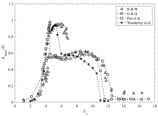
Figure 9.
The variation with the reduced velocity of the normalized maximum structural amplitude () of FIV consisting of an elastically-mounted circular cylinder of diameter D with a mass ratio of 2.4 and mass-damping ratio of 0.013. The results of three RANS modelling studies are compared with some experimental data reported by Khalak and Williamson [159] (K&W). The RANS modelling studies shown here were conducted by Guilmineau and Queutey [160] (G&Q), Pan et al. [161], and Wanderley et al. [162].
Guilmineau and Queutey [160] applied RANS with the shear stress transport (SST) k- model to investigate the influence of initial conditions on the transverse VIV of a circular cylinder for flows with Reynolds number ranging from 900 to 15,000. A key result reported in this modelling study is that initial conditions of rest and of decreasing velocity reproduced the two-branch VIV response (initial and lower), while that of an increasing velocity yielded a very narrow upper branch with an amplitude that is comparable to the experimental data. Applying the same numerical methodology as used in Guilmineau and Queutey [160], Pan et al. [161] focused their attention on the reason for failure of RANS modelling to correctly predict the upper branch of the VIV response. These researchers suggested that the reason was related to the random (stochastic) behavior of the vortex-shedding process which cannot be achieved using a time-averaged (or ensemble-average) RANS modelling strategy. Wanderlay et al. [162] applied RANS with the k- turbulence closure model and demonstrated that this approach was able to provide very accurate predictions of the three branches of VIV response, of the force coefficients, and of the lock-in range.
Zhao and Cheng [92] conducted RANS modelling of the streamwise and transverse VIV of a rigid circular cylinder of diameter D and correctly predicted the characteristic behavior of the super-upper branch of the VIV response—a maximum amplitude of when the flow velocity is increasing. These researchers also reported three vortex shedding modes of VIV in the near-wall region based on their RANS modelling study. Some numerical studies apply RANS modelling to investigate the influence of the Reynolds number on the VIV response of a circular cylinder. Wanderlay and Soares [163] used RANS to model the 1DOF-VIV response of a circular cylinder at a small mass-damping parameter for three different ranges of the Reynolds number (namely, Re = 2000–6000, 2000–12,000, and 2000–24,000) and for six fixed values of the Reynolds number (namely, Re = 100, 200, 300, 400, 1000, and 1200). It was found that the Reynolds number has a significant effect on the amplitude response, the lift coefficient, and the vibration frequency for a low mass-damping system and that the upper branch of the VIV response only appears as the value of Re is varied, but not for a fixed value of . This study suggests that the combined influence of Re and on the VIV response requires more investigation.
Recently, Gu et al. [164] applied RANS with the SST k- model to study the effect of Reynolds number on the VIV response at small and moderate values of Re. A non-dimensional parameter was defined in order to deal with the combined influence of Re and on the VIV response—a parameter that can be varied by changing the flow velocity, the cylinder diameter and the structural stiffness while ensuring that the values of the mass and the damping ratio are fixed. These researchers concluded that the VIV response is sensitive to the Reynolds number for moderate values of Re and, indeed, it was shown that the maximum amplitude of the VIV response is strongly dependent on Re. Kang et al. [165] used RANS to study Re effects for a 2DOF-VIV consisting of a circular cylinder at small and large mass ratios for three different Re ranges: namely, Re = 1450–10,200, 5800–40,800, and 13,050–91,800. With respect to the influence of mass and damping on the VIV response, Khan et al. [166] and Anwar et al. [167] used RANS with the SST k- turbulence closure to model the transverse VIV response of a circular cylinder with a mass ratio of 11 at Re = 10,000. These researchers demonstrated that RANS can be used to correctly predict the three branches and vortex modes in the VIV response for higher mass ratio at a high-Reynolds number—albeit the peak amplitude within lock-in range was underestimated. Martins and Avila [168] investigated different combinations of the structural damping ratio and the Reynolds number on the VIV response using the RANS SST k- model.
The studies summarized above involve RANS modelling of the VIV of an elastically-mounted circular cylinder. However, RANS modelling has also been utilized to predict the FIV of bluff bodies with more complex (non-circular) cross-sectional shapes. Cui et al. [169] used 2D RANS modelling to investigate the transverse FIV of square and rectangular cylinders for different inflow angles at moderate values of the Reynolds number. These investigators reported that galloping is induced on the square cylinder at an inflow angle of 0 and on the rectangular cylinder at inflow angles of 0 and 90. Han et al. [170] employed 2D RANS to model the power performance of a low-mass square energy harvester based on an 1DOF-FIV (VIV and galloping) at Re = 24,000–160,000 and investigated the effect of the inflow angle and the structural damping ratio on the FIV response. One interesting phenomenon observed in this study was that a large-amplitude response occurs at large value of for the square cylinder, regardless of the value of the inflow angle (0, 22.5, and 45) or mode of response (viz., whether VIV or galloping). Other notable studies using 2D RANS modelling to investigate the FIV response of non-cylindrical bluff bodies include Ding et al. [171] (for square, triangular, quasi-trapezoidal shaped bodies), Zhang et al. [172] (for triangular, square, pentagonal, circular-shaped bodies), Zhang et al. [173] (for triangular, square, hexagonal, octagonal, 24-sided, circular shaped bodies), and Wang et al. [174] (for different rear edges such as semicircular, triangular, trapezoidal, rectangular). In these studies, the RANS modelling provided predictions that agreed well with experimental data in terms of the FIV response. Most of these studies also determined the power production arising from the FIV of different shapes of the bluff bodies in order to provide practical guidance for the design of a FIV energy harvester.
RANS modelling can be used to predict the dynamic response of a cylinder with PTC involving, in particular, attached or detached appendages having more complex and/or irregular geometric structure. To this purpose, Zhu and Yao [175] used 2D RANS to show that the correct placement of multiple small rods around an elastically mounted circular cylinder can result in a significant suppression of the streamwise and transverse VIV response. With respect to the incitement of oscillatory motion, Ding et al. [176] used 2D RANS with the Spalart–Allmaras (SA) turbulence closure to model the FIV response of a rigid circular cylinder of diameter D with two roughness strips for flows at high-Reynolds numbers in the range from 30,000 to 110,000. These researchers showed the presence of a five-branch FIV response for this configuration (viz., static, VIV initial, VIV upper, transition from VIV to galloping, and galloping). Furthermore, it was shown that the maximum amplitude was increased due to the presence of the roughness strips—indeed, the maximum amplitude was as large as 3.5 D. Another parametric study was conducted by Wang et al. [177] who showed that attaching two symmetrical small-diameter cylindrical rods at angular locations of 55 to 65 around the circumference of the cylinder significantly extended the range of aeroelastic instability of the vibrating system.
Zhao and Cheng [93] used RANS with the SST k- model to study a 2DOF-VIV system consisting of a rigidly connected four-cylinder square configuration arranged with a fixed center-to-center separation. The modelling was undertaken for flows with Reynolds numbers in the range Re = 1000–20,000. A key result of this study was that the inflow angle of the incident flow has a significant effect on the lock-in range, the mode of vibration of the amplitude response, and the hydrodynamic force coefficients. RANS modelling has been used to investigate the transverse VIV of a two-cylinder system, such as two rigidly coupled side-by-side cylinders with different diameters [178], side-by-side and tandem arrangements of cylinders [179], and two elastically coupled side-by-side cylinders in symmetric and asymmetric configurations [180].
Table 4 provides a summary of a number of important studies involving the use of RANS modelling to predict the FIV response for single or multiple bluff bodies of various shapes (single cylinder, cylinder with PTC, array of cylinders). Some studies included here involve very complicated FIV responses, especially those for flows in the subcritical Reynolds number regime.
Table 4.
Summary of a number of representative RANS modelling studies of flow-induced vibration of bluff bodies.
4.6. Detached-Eddy Simulation (DES) of FIV
To strike a balance between simulating (resolving) and modelling turbulence, detached-eddy simulation is a hybrid LES/RANS approach that can be used to predict the flow over a stationary or vibrating cylinder. DES involves modelling the small-scale (unresolved) turbulence in the near-wall regions of the flow with a sufficiently fine grid using RANS and simulating (resolving) the turbulent flow in the regions away from the wall using a grid that is appropriate for LES. The governing equations of DES can be written in a general form applicable for both RANS and LES depending on how the mean quantities are defined (viz., ensemble-averaging for RANS and spatial filtering for LES). DES is more applicable for the simulation of highly separated flows in the high-Reynolds number regime at a computational cost that is intermediate between those of LES and RANS.
Nguyen and Nguyen [181] used a DES based on the SST k- model to simulate an 1DOF-VIV system consisting of a single circular cylinder subjected to free (undisturbed) incident flow and a 2DOF-VIV system consisting of a downstream cylinder subjected to the wake flow generated in the upstream direction by a fixed cylinder. Both cases involve a high-Reynolds number flow. These investigators reported a very good agreement of their predictions with experimental data and suggested that DES yielded more accurate predictions of the fluid forces, the VIV response and the phase difference than a comparable 2D RANS model. Joshi and Jaiman [182] applied the delayed detached-eddy simulation methodology to simulate the VIV of a slender flexible riser immersed in a turbulent flow at a subcritical Reynolds number. In this study, the response amplitudes and the motion trajectories were found to be in good agreement with the experimental measurements. Recently, Ma et al. [183] used DDES to investigate FIV associated with a cylinder with passive turbulence control (involving, as such, attachments of two strips to the cylinder of different thickness at different locations to give different coverage). Their numerical results agreed very well with the experiment data and successfully reproduced almost all the key features of the FIV response, such as the maximum amplitude, the multiple branches in the response, and the vortex shedding modes. Another similar DES study was conducted by Ma et al. [184] but for a flow at the lower Reynolds number of Re = 3900.
Table 5 summarizes the details of these DES studies of FIV phenomena. Generally speaking, this body of work suggests that DES is a very promising methodology for the prediction of the FIV response for rigid/flexible circular cylinders and and for cylinder–appendage system at high-Reynolds numbers.
Table 5.
Summary of some key DES studies of the flow-induced vibration of bluff bodies.
5. Machine Learning and FIV
The numerical modelling described in Section 4 is a full-order model (FOM) based on the numerical solution of various forms of the Navier–Stokes equations coupled with an equation of motion for the structure (body). This is a useful strategy to study the FIV of a bluff body, but is limited to low-Reynolds number flow (if DNS is used) or requires significant computational resources for flows in the strongly turbulent regime at very high Reynolds number. Furthermore, as noted by Hollenbach et al. [185] and by Sanders [186], the traditional CFD technology has no ability to provide physical insight into the mechanism underpinning the FIV behavior.
Fortunately, the recent advancements in data-driven modelling based on machine learning make it possible to address the issue of the high computational cost of conducting CFD simulation/modelling of FIV phenomena. Data-driven modelling using machine learning can be applied in two different contexts: (1) construction of a reduced-order model (ROM) of the FIV phenomena (viz., a simple mathematical representation of the principal characteristics of the full-order model based on CFD) as discussed in Section 5.1; and (2) use of a deep neural network (DNN) either to accelerate the conventional numerical solution of CFD or to map the non-linear relationship between inputs (e.g., flow and structure properties) and outputs (e.g., dynamic response, FIV forces, wake patterns) as described in Section 5.2.
For readers who may not be familiar with machine learning, we will provide a brief introduction to certain machine learning techniques that have been applied to modelling FIV phenomena (described later in this section). Machine learning is a rapidly developing discipline that lies at the intersection of computer science, statistics, and applied mathematics. Machine learning algorithms are data-driven in the sense that these algorithms are used to generate models from data—as more data are used, the models can improve. From this perspective, machine learning can be used in any data-rich field (more specifically, for the modelling of FIV phenomena considered herein) that generates a great amount of data (big data).
In the application of machine learning to FIV modelling, the non-linear dynamical system that generates the relationship between the inputs (e.g., flow) and output (e.g., transverse displacement) is characterized through the training data. Machine learning algorithms can be used to build input–output models using time series data obtained from either experimental measurements or numerical simulations of the dynamical system. Examples of such machine learning algorithms are the autoregressive with exogenous input model (and various extensions), the eigensystem realization algorithm (ERA), and the dynamic mode decomposition (DMD)—all of which will be described below as it applies to unravelling the dynamics associated with FIV phenomena. These methodologies can be interpreted as model reduction methods that generate a low-dimensional representation of the complex input–output relationship of the dynamical system from black-box data streams (e.g., a series of “snapshots” or solutions obtained from a numerical simulation of the dynamical system).
Other machine learning techniques include artificial neural networks (ANNs) (and, more specifically, deep neural networks (DNNs)) as depicted in Figure 10a which consist of a number of individual computational units (neurons) organized in a number of successive layers. The computational units of the network are connected in a graph structure. A DNN (unlike a shallow neural network) contains multiple computational layers—the intermediate layers between the input and output layers are referred to as hidden layers with the nodes in one layer connected to those in the next layer (in a architecture known as a feedforward network). The output of the j-th computational unit (neuron) in the l-th layer of a DNN (each layer of which consists of n neurons) is given by
where is output of the r-th neuron in layer s, is the weight that connects the i-th neuron in layer to the j-th neuron in layer l, is the bias imposed on the j-th neuron of layer l, and is a non-linear activation function. Typical activation functions include the sigmoid function and the rectified linear unit (ReLU) function . The neural network has a number of unknown parameters, namely the weights and biases, whose values are obtained by the neural network model so that it provides a good fit to the training data (without overfitting these data so that the model generalizes well—viz., gives good predictions of data not used in the training process). Usually, these parameters (weights and biases) are determined by modifying their values using a gradient descent algorithm to minimize a loss (or error) function that provides a quantitative measure of the performance (or accuracy) of the neural network predictions on the data.
Figure 10.
The architecture of a deep neural network (DNN). (a) A general deep neural network consisting of a number of computational units (neurons) organized into a number of layers and connected in a graph structure [187]. In this example, the neural network of an input layer having two neurons (viz., input X is a two-dimensional vector), an output layer with one neuron (giving a prediction of the output ) and four hidden layers that pass information from a previous layer into the next layer. (b) A physics-informed neural network (PINN) with an input t, an output , and two hidden layers with four neurons each [188].
A variant of DNNs is the so-called physics-informed neural networks (PINNs), an example of which is exhibited in Figure 10b. A PINN is an example of a scientific machine learning technique which integrates both data and mathematical physics models (physical constraints and domain knowledge) in the learning algorithm. The mathematical physics model (usually expressed as a partial differential equation) is embedded into the loss function of the DNN using automatic differentiation. More specifically, the loss function of a PINN consists typically of the weighted losses of the data and the partial differential equations encoding the underlying physics of the problem. The PINN is then trained by minimizing the loss using a gradient-based optimizer just as for the physics-uninformed neural network (see Figure 10a).
5.1. Data-Driven Reduced-Order Models (ROM) of FIV
Reduced-order modelling in the context of fluid dynamics involves the development of a low-dimensional mathematical model from a large flow dataset obtained either from experimental measurements or from full-scale CFD simulations. The unsteady aerodynamic models can be divided into three classes [189]. Firstly, there are the purely linear models where the static and dynamic aerodynamic forces acting on the body are linear—these models are most useful for steady or quasi-steady flows. Secondly, there are dynamically linear models where the flow is non-linear in space, but adheres to a linear relationship in time (also referred to as a time linearization model). A projection-based ROM and a system identification-based ROM are examples of this kind of model. The latter type of ROM is typically used to characterize an unsteady flow past a structure subject to a small disturbance (perturbation). Thirdly, there are the dynamic non-linear models. With an increase in the amplitude of motion, the aerodynamic characteristics of the dynamic non-linearity reveals itself and the implicit assumption of a small disturbance (perturbation) is no longer valid. Dynamically linear and non-linear models are frequently used to represent the FIV response of bluff bodies.
5.1.1. Projection-Based ROM
Proper orthogonal decomposition (POD) [190] and dynamic mode decomposition (DMD) are two methodologies that are used to construct a projection-based ROM. The datasets that are used to construct this type of ROM are sequences of snapshots of the flow field (e.g., velocity, pressure). This type of ROM is frequently used to study the characteristics of coherent wake structures in a flow.
The proper orthogonal decomposition (as referred to as principal components analysis in the statistical literature) has been used in conjunction with the Galerkin projection method to construct a reduced-order model. This consists of two steps: namely, (1) determine a low-dimensional subspace where the dominant dynamics occur by decomposing a high-dimensional flow field (assembled as a data matrix X) into a set of orthogonal modes; and (2) project the high-order Navier–Stokes equations (partial differential equation, PDEs) that determine this high-dimensional flow into this low-rank subspace to obtain a system of ODEs using a Galerkin projection methodology [191,192]. It is noted that POD is an efficient method for model order reduction in the flow dynamics of a system—it involves computing the singular value decomposition (SVD) of the data matrix X and using the information contained in the decomposition to construct the optimal basis modes (optimal POD modes) that can be used to extract a low-rank, low-dimensional subspace of dynamic flow evolution. Following from this analysis, it is possible to approximate the flow field evolution given the NS equations using a Galerkin projection of the NS equations onto the optimal POD modes to give the dimensionally reduced evolution equations.
One common shortcoming of the conventional POD/Galerkin methodology is the lack of a clear separation of the individual dynamics embodied in the optimal basis modes—this makes it difficult to build a high-quality ROM [193]. Moreover, certain low-energy components that do not contribute to POD modes can have a large influence on the underlying mechanisms responsible for the flow features, implying that the POD-based ROM may provide poor predictions in this case. As a result, many variants of the conventional POD/Galerkin methodology have been developed to mitigate these shortcomings, such as the balanced POD (BPOD) [194] and the spectral POD (SPOD) [193].
Recently, Schubert et al. [195] developed a data-driven ROM based on SPOD and applied it to reconstruct the turbulent wake dynamics of a circular cylinder undergoing VIV at Re = 4000. These researchers applied a sparsification procedure to determine the temporal coefficients corresponding to the POD modes and enhanced the reliability and robustness of the ROM.
Rather than basing a decomposition on the energy content of orthogonal modes while ignoring the temporal information as in POD, DMD provides a modal decomposition of the high-dimensional flow structures, where each mode in the decomposition embodies spatially correlated structures that have the same linear behavior in time—in so doing, the DMD provides not only a dimensionality reduction as in POD but also gives a model for the time evolution of these modes. Each DMD mode corresponds to a single complex frequency (oscillation that grows or decay) which is useful for providing a deeper understanding of the flow mechanism, as well as for stability analysis. Moreover, the eigenvalue/eigenvector decomposition provided by the DMD modes provides the flow evolution, obviating the need to apply the Galerkin projection to obtain the dimensionally reduced evolution equations for the dynamical system. As an example, Kou et al. [196] employed DMD to investigate the temporal evolution of the purely fluid modes at Reynolds numbers between 12 and 55—this information was used to explain the occurrence and disappearance of VIV phenomenon in the subcritical regime.
5.1.2. System Identification-Based ROM
Another time-linearized ROM uses system identification to unravel the dynamical relationship between the input and output data—two common data-driven methodologies based on this approach are the autoregressive with exogenous input (ARX) model and the eigensystem realization algorithm (ERA).
The key steps for the development of a system identification-based ROM are: (1) perform full-order CFD simulations in order to obtain the required high-fidelity input-output datasets; (2) train the unsteady fluid dynamics ROM, using either the ARX or ERA methodology based on the data collected in the previous step; (3) couple the equation of motion for the structure with the data-driven model to give an unsteady coupled ROM for the (total) FSI system; and (4) conduct a linear stability analysis (LSA) of the dynamical system using the coupled ROM. Note that either ARX or ERA is used to derive the ROM for the fluid dynamics in step (2)—the other three steps are the same for both methodologies.
The ARX model is a linear time series model based on a discrete difference equation for the input–output data, in which the current system output is expressed as the linear superposition of the current input, as well as previous (in time) inputs and outputs, so
where the input u and output are obtained from full-order CFD simulations. The time delay order parameters and are specified by the user and the model coefficients () and () need to be estimated (either through a least-squares fitting process or application of the maximum likelihood procedure). The development of an unsteady fluid ROM based on ARX consists of four steps: (1) compute the steady-state base flow for the FIV system (subject to a specific input signal) using a numerical solver; (2) estimate the ARX model coefficients and defined in Equation (33); (3) construct the reduced matrices using the estimated values for and ; and (4) recast the fluid dynamics ROM into a standard state-space format.
In general, a unit step signal can be used as the input (training) signal for computation of the steady-state base flow. The requirement is that the prespecified training signal should be persistently exciting (viz., its spectrum should contain a sufficiently large number of harmonics) so that the input can trigger the unsteady linear flow dynamics. In the context of the FIV response of a bluff body, the single input and output can be taken to be the transverse displacement of the cylinder and the instantaneous lift coefficient acting on the cylinder, respectively. The application of ARX to better understand FIV phenomena has described in [197,198,199,200]. More specifically, Zhang et al. [197] constructed a fluid ROM using ARX and this data-driven model is then coupled to the structure equation. This coupled ROM for FSI was used to investigate the physical mechanisms underlying the frequency lock-in in VIV for a flow at Re = 60. Utilizing linear stability analysis of VIV based on the coupled ROM, these researchers reported two lock-in patterns: namely, a “resonance-induced” lock-in (only the wake mode is unstable) and a “flutter-induced” lock-in (both the wake mode and the structure mode are unstable). Moreover, Zhang et al. [197] also investigated the effect of the natural frequency, the mass, and the damping of the cylinder on the VIV dynamics using the FSI ROM. The main results concerning lock-in of VIV reported by Zhang et al. [197] were further confirmed by other global LSA studies (e.g., Navrose and Mittal [201] applied LSA using a linearized Navier–Stokes equations in which the equations for the steady flow and disturbance field were obtained separately).
The intrinsic mechanisms of various FIV response have been investigated using ARX in conjunction with LSA. These include investigations of the transverse galloping of a square cylinder in laminar flow (at Re = 140–180) [199], the wake-induced vibration of two identical tandem cylinders at Re = 60 [198] and the VIV suppression of a circular cylinder by a tuned mass damper [200].
The eigensystem realization algorithm (ERA) is a data-driven methodology originally presented by Juan and Pappa [202] who used it to identify modal parameters relevant to modelling structures on the space shuttle. ERA is a linear system identification methodology that uses the impulse response of the system to construct a ROM for the dynamics. The development of a fluid ROM using ERA consists of the following key steps: (1) calculate a steady-state base flow subject to an input impulse response using a numerical solver; (2) use this impulse response data to construct a generalized Hankel matrix H obtained by stacking shifted time sequences of the data; (3) compute the singular value decomposition (SVD) of H; (4) calculate the reduced system state matrices; and (5) recast the fluid ROM into a state-space format. In ERA, the dimension of the Hankel matrix H is a critical parameter that controls the convergence of the constructed ROM.
In greater detail, ERA is applied with reference to a discrete-time state-space system with the form
where , , and are the state vector, input vector, and output vector at discrete time step i; and, A, B, C, and D are the system, input, output, and feed-through matrices, respectively. ERA uses measurements of the impulse response of a dynamical system to infer the matrices (A, B, C, and D) that define the state-space model. To this purpose, a discrete Kronecker delta function input of the form
(I is the identify matrix and is the time-step size) gives rise to the impulse response (output of the dynamical system) in the form
This impulse response data are used to form a Hankel matrix H obtained by stacking shifted time series of the data to give
Next, we take the SVD of H, truncate the small singular values in this decomposition (viz., retain only the dominant singular values), and create a second shifted Hankel matrix H’ (obtained by shifting the columns of H one time step to the left). The information in the truncated SVD and in H’ can be used to construct estimates for (A, B, C, and D) that define the discrete-time state-space model (reduced-order model) of the dynamical system.
Jaiman and colleagues conducted number of investigations of the FIV response of a bluff body using the ROM/ERA methodology [203,204,205,206,207]. Yao and Jaiman [203] conducted LSA on the transverse VIV of a circular cylinder. These researchers then investigated the stability characteristics of FIV of a cylinder having different cross-sectional shapes (e.g., ellipse, forward triangle, diamond, and squares with various rounding radii). Generally speaking, these results demonstrated the effectiveness of using ROM/ERA to predict various features of the FIV phenomenon. Indeed, ROM/ERA has been used to conduct stability analysis of various vibrating systems, such as the FIV of a cylinder with different passive suppression devices (e.g., fairings, splitter plate, connected-C) [206], of two cylinders in either a tandem or side-by-side layout [205], and of active control of the VIV of a circular cylinder [204] and a sphere [207].
The most useful aspect of the ARX and ROM/ERA methodologies is that once the ROM is obtained using the data-driven process, it is straightforward to perform a linear stability analysis of the dynamical system—an analysis that facilitates deeper insights into the underlying mechanisms responsible for FIV through the examination of eigenvalue trajectories (which allows one to better understand the competition between structure and wake modes). For example, Cheng et al. [208] investigated the modal interaction and transformation of a VIV system consisting of the flow past an elastically-mounted circular cylinder for Reynolds numbers in the range from 20 to 180. These researchers used ERA/ROM the explain the beating phenomenon observed in VIV which occurs in the initial branch of the response and the significant lag time that arises between the initial branch and the occurrence of a fully developed response in the lower branch. Other relevant investigations utilizing LSA in the context of ROM/ERA in order to better understand the FIV phenomenon include Bukka et al. [206], Yao and Jaiman [204], Chizfahm and Jaiman [207], and Li et al. [199].
It is important to stress that the linear ROMs constructed using ARX or ERA cannot be employed to study the non-linear characteristics of the flows associated with the FIV phenomenon.
5.1.3. Non-Linear ROM
The projection-based ROMs based on either POD or DMD and the system identification-based ROMs based on either ARX or ERA are linear models of the system dynamics (viz., they are time-linearized, dynamically linear or statically non-linear [209]). One common weakness of these approaches is that they are difficult to generalize to high-dimensional non-linear systems involving large-amplitude motions of the structure such as the FIV response of a bluff body subjected to a strongly turbulent flow.
In order to predict the non-linear dynamics of a complex flow system using a ROM, a general strategy is to incorporate within the linear model some mechanism to account for non-linearities in the dynamics, such as the Koopman operator [210] and the discrete empirical interpolation method (DEIM) [211]. In particular, Miyanawala and Jaiman [211] combined POD and DEIM to present a non-linear ROM for the 2DOF-VIV of a sharp-cornered square cylinder immersed in either a laminar or turbulent flow. These researchers successfully used this non-linear ROM to interpret the most significant wake features and their contributions to the forces on the vibrating body.
An alternative for the generation of a reduced-order non-linear model of a high-dimensional flow field uses machine learning, especially deep neural networks. Some DNN architectures can be interpreted as non-linear generalizations of either POD or DMD in the sense that they decompose the high-dimensional flow fields into low-dimensional non-linear modes. An example is provided by the convolutional neural network (CNN) autoencoder proposed by Murata et al. [212]. Another strategy is to combine a DNN with a traditional linear model decomposition in order to construct a hybrid ROM that integrates the linear and non-linear characteristics of an unsteady flow. The conventional POD performs well in dimensionality reduction based on a set of time-invariant orthogonal modes. As a generalization, the temporal evolution of the POD modes (represented as modal coefficients) can be learned using a deep neural network—examples include the CNN [213] and the encoder–decoder recurrent neural network (RNN) using a long short-term memory (LSTM) cell [214]. The effectiveness of these hybrid POD-DNN-based ROMs has been demonstrated by their successful prediction of various aspects of the FIV of a bluff body for flows at low- and high-Reynolds numbers.
In order to identify non-linear low-dimensional features of a flow, Bukka et al. [215] incorporated a CNN with an RNN to give a convolutional recurrent autoencoder network (CRAN) model. In this framework, a low-dimensional embedding of the state variables was learned by the CNN and the transient evolution of the dynamics was learned using the RNN-LSTM. A conventional linear system identification technique can also be combined with a DNN and used to investigate the underlying mechanism and stability characteristics of a strongly non-linear dynamical system. To this purpose, Kou and Zhang [209,216] proposed a hybrid ROM to accurately predict the integrated flutter and buffeting of an airfoil. Here, an ARX model was trained and used to approximate the linear dynamics while the non-linear deviations between the real outputs for large-amplitude inputs and the ARX model was represented using a radial basis function neural network (RBFNN). In the context of predicting the VIV of a freely vibrating sphere in the transverse direction, Chizfahm and Jaiman [217] used a predictive RNN-LSTM as a DNN-ROM to provide the non-linear mapping of the input-output dynamics of the FSI system. This was integrated with a ROM/ERA to provide a linear approximation of the non-linear model for the stability prediction.
5.2. Data-Driven Deep Neural Network Applied to FIV
Recent advancements in using machine learning within the broader field of fluid dynamics [3] can be applied for the specific problem of simulating FIV. The possible application modes can be divided into three types: (1) use machine learning to augment the numerical solving procedure in standard CFD solvers; (2) use deep neural network to infer the flow field and FIV response; and (3) use deep neural network to model the fluid force of FIV. The above three applications are all data-driven methods, which will be reviewed in detail below.
Deep learning is a subset of ML that refers to the use of highly multi-layered neural networks to understand a complex dataset, with the intention of predicting certain features in the dataset.
5.2.1. DNN-Accelerated Fluid Modelling
The first scenario integrates the machine learning technique into the standard CFD solver to accelerate the key calculation steps. This is a hybrid application of traditional CFD simulation and learned neural network in fluid dynamics. Duraisamy et al. [218] reviewed various machine learning methods for augmenting numerical simulation techniques at various levels of fidelity.
High-fidelity simulations of FIV require the use of DNS or of LES. While DNS simulations of high-Reynolds number turbulent flows is prohibitively expensive, recent advancements in applying machine learning to perform accurate DNS on a coarser grid greatly reduce the computational expense [219]. In DNS, a major computational burden is resolving the smallest physical scales in the flow through the use of extremely fine grids. In order to accelerate the computation of DNS and LES without loss of accuracy, Kochkov et al. [219] embedded a neural network interpolator into the standard CFD solver on a coarser grid—specifically, in order to approximate the convective flux term for DNS and model the residual correction for LES. The training dataset is high-resolution simulations for Kolmogorov flow at Re = 1000. In this application, the isotropy of Kolmogorov flow particularly lends itself to this methodology and the training procedure and model structure can benefit from numerous invariances in this flow. In principle, the ML-based CFD solver proposed by Kochkov et al. [219] can be applied to any flow since the output of the neural network only depends on local features, which was validated by a test case with large-domain size, decaying turbulent flow and a higher Reynolds number of 4000.
The traditional turbulence modellings in CFD apply some approximations for turbulence effects at high-Reynolds numbers, such as a SGS model in LES or the SST k- model in RANS, which is the main source of numerical errors. Therefore, an alternative way to improve the accuracy of simulations and to speed up the calculation of LES and RANS is to modify the Reynolds stress or SGS stress through the application of machine learning techniques. A notable machine learning technique within the field of LES is the neural network SGS model of Maulik et al. [220], which allows for a more accurate closure within LES. Compared to LES, machine-learning augmented RANS is a broad and rapidly developing field. Several techniques have been developed to accelerate RANS modelling and increase their accuracy. A popular approach is to integrate a richer eddy viscosity closure relationship. For example, Ling et al. [221] used a tensor basis neural network (TBNN) to predict the anisotropy tensor, a highly versatile closure relationship. Another notable work in augmented eddy viscosity modelling includes the framework proposed by Wu et al. [222].
The application of machine learning mentioned above is interpreted from an overall perspective of fluid dynamics, focusing more on the general approaches instead of application to a specific problem. There is no doubt that these ML-based techniques, regardless whether it is the ML-accelerated DNS/LES, or the ML-modified turbulence modelling of LES/RANS, could in principle be used to address numerically the FIV response of a bluff body, increase the accuracy of LES/RANS simulation, or develop a highly-tuned LES/RANS model for turbulent FIV simulations.
5.2.2. Physics-Informed Neural Network of FIV
Contrary to the ML-based DNS or LES or RANS models, the second application of machine learning in fluid dynamics is completely out of the traditional CFD simulations—that is to say, no numerical calculations are needed during the inference procedure by a trained deep neural network. It should be noted that the training dataset can be experimental data or numerical results—if it is the latter, the necessary CFD simulations would be carried out during the data preparation period. This data-driven deep learning technique has been employed explicitly for modelling the FIV response of a circular cylinder.
Raissi et al. [188] conducted some seminal work to apply a physics-informed neural network (PINN) model to accurately infer the lift and drag forces acting on a circular cylinder undergoing a 1DOF-VIV from scattered simulation data of the velocity field for a laminar flow at . It should be noted that the PINN presented by Raissi et al. [188] is not a black-box model like traditional data-driven neural networks based on large training data, because it encodes the NS equations coupled with the structural motion equation into the loss function as regularization (constraints on the output of the neural network), which makes it have potential to infer target variables based on the governing physical laws and on a limited training dataset. Inspired by the introduction of the eddy viscosity in conventional turbulence models used in CFD (e.g., LES, DES, RANS) for the closure of either the time-averaged or spatially-filtered NS equations, Xu et al. [223] introduced an artificial viscosity in the RANS framework to formulate the parameterized Navier–Stokes equations, which was treated as the physical constraint of the established PINN. For the case of flow over a stationary cylinder at a high-Reynolds number of , the physics-informed deep learning successfully reconstructed the missing flow dynamics and inferred the lift and drag coefficient profiles. As an extension of the study reported by Raissi et al. [188] and by Xu et al. [223], Bai and Zhang [224] further used both the parameterized Navier–Stokes equations-based PINN (PNS-PINN) and the Navier–Stokes equations-based PINN (NS-PINN) to infer the unsteady velocity field and force coefficients for the transverse VIV of a circular cylinder in a turbulent flow. The training data for neural network models consisted of 2D RANS data at Re = 10,000 and employed the SST k- model and the SST-SAS turbulence closure models. These researchers also tested two kinds of datasets based on the flow velocity and the dye trace, respectively. The results demonstrated the predictive capability of the PNS-PINN trained by a velocity dataset for turbulent VIV at subcritical Reynolds numbers, in terms of correctly predicting the flow field and the lift and drag coefficients. Cheng et al. [225] applied a similar PNS-PINN approach to study the 2DOF-VIV of a single circular cylinder at Re = 2889 and wake galloping of two rigidly-connected circular cylinders at Re = 9000 and reported good success.
The above four representative studies have demonstrated that the data-driven deep learning technique underlying the PINN framework is capable of inferring the complicated FIV response of a bluff body from a limited training dataset, in terms of dynamic parameters (damping and stiffness), the entire velocity and pressure fields, and the lift and drag forces acting on the vibrating system. Moreover, PINN can be applied in various scenarios, from laminar to turbulent and for a single cylinder or multiple (array of) cylinders.
5.2.3. DNN-Based FIV Force Model
The last machine learning model is specialized in predicting the FIV modelling of a bluff body, which involves some small-scale numerical calculations, not for the NS equations (multiple PDEs) governing the fluid dynamics, but for the mass–spring–damper (one ODE) system controlling the structural oscillation.
As an example of this approach, we focus on a recent work by Zhang et al. [187] which will be explained in detail in order to help the reader understand what role machine learning plays in the VIV prediction for a single circular cylinder. As shown in Equation (13), the forcing term on the right-hand side represents the fluid force responsible for the VIV response of a circular cylinder, which is closely related to the flow properties and the vibration parameters. Zhang et al. [187] established a deep neural network to map the relationship between these two, which has as the aerodynamic force coefficient as the single output and multiple input features, such as the Reynolds number, the reduced velocity, the oscillation amplitude and the velocity of the circular cylinder, as well as a few parameters characterizing the oscillating incident flow. The neural network was trained using a large dataset from forced-vibration experiments. To predict the transverse VIV of flexible pipes, the trained neural network was applied to calculate the fluid force at each time instant, which was then substituted into Equation (13), so that this second-order ODE can be numerically solved. This was accomplished by using the Newmark- method combined with a finite-element discretization of the long flexible pipe. Another similar case will be given in Section 6 for a VIV energy harvester.
It can be inferred that the excitation force coefficient model based on a deep neural network is computationally efficient owing to the fact that the calculation of the mass–spring–damper system is much simpler than the solution of the NS equations in the first scenario.
6. Energy Harvesting Based on FIV
Section 2, Section 3, Section 4 and Section 5 have provided a comprehensive overview of the various methodologies that can be used to model the FIV response, such as mathematical modelling, numerical modelling, and modelling based on machine learning approaches. Flow-induced vibration is essentially a FSI phenomenon and a deeper understanding of this phenomenon is important for real-world engineering and industrial applications—the most common is perhaps the control (suppression) of FIV in engineering structures such as offshore production risers [226], heat exchanger tubes [227], suspension bridges [228], and power transmission lines [229]. The efficient harvesting of the energy potential of FIV is a key application arising from the growing demand for clean and renewable energy, as well as the rapid development of related technologies, such as wireless sensor networks and micro-electromechanical systems [7,230]. This section focuses on recent advancements in flow-induced vibration energy harvesting (FIVEH)—this application is used to illustrate how the various modelling methodologies described earlier can be used to address this important problem.
The concept of FIVEH is to harness wind and/or water energy from the surrounding environment by utilizing structures that oscillate in the flow (providing various FIV responses) and then converting this energy of oscillation into usable energy (e.g., electricity). Therefore, FIVEH primarily involves two forms of coupling: namely, (1) the bidirectional fluid–structure interaction converting fluid energy to mechanical energy and (2) the electro-mechanical coupling transforming the mechanical energy to electrical energy. The former specifically refers to various FIV phenomena (see Section 2) consisting primarily of VIV and galloping. The oscillatory energy arising from the FIV response can be converted by various means—electromagnetic, piezoelectric, electrostatic, dielectric, triboelectric, interface circuit, and power management [6]—to a usable form of energy.
Like other energy generators, the core research objective of FIVEH is to obtain the optimal power performance—specifically, to enhance the oscillation by widening the effective flow speed range and reducing the cut-in velocity of FIV so as to maximize the energy harvesting efficiency and power generation. The performance of FIVEH can be directly evaluated by the output voltage, or indirectly analyzed by examining critical oscillation properties, such as the displacement amplitude, the vibration frequency, and the lift force acting on the moving body.
Numerous efforts have been made to enhance the power performance of a FIV energy harvester in a number of ways. The most direct and easiest way is to change the geometrical shape of the bluff body which can include utilizing a cylinder with a non-circular cross-section (e.g., square cylinder [231], rectangular cylinder [232], triangular cylinder [233], D-section cylinder [234]) and incorporating a PTC device to change the surface roughness of the cylinder (e.g., adding attachment(s) to a cylinder, such as roughness strips [176], trip wires [235], a splitter plate [236], small rods [237], and a free-to-rotate impeller [238]). The underlying strategy here is to obtain an asymmetrical geometry of the rigid body which induces an instability in the shear layer to produce a negative damping in the transverse (crosswind) direction and, hence, trigger galloping on the vibrating body. As mentioned in Section 2.3, an energy harvester driven by galloping can potentially yield a larger power production than that driven by VIV. In addition to incorporating appendages on an oscillating body, the non-linear spring stiffness and damping can be changed on the supporting structure to improve the harvested power and efficiency [239,240]. The mechanical part of the energy harvester can also be designed as a dual-mass system (i.e., one mass undergoing FIV is used to drive another mass with an attached magnet that moves relative to a coil in order to produce electricity [241]), as a multi-degree-of-freedom system [242], and as a multi-directional system [243]. All these strategies have been shown to improve the extraction of fluid energy from the ambient flow. Moreover, an hybrid energy harvester based either on two or more FIV phenomena (e.g., VIV-galloping) or on utilizing multiple forms of renewable energy simultaneously (e.g., wind, water, photovoltaic) based on multiple energy conversion mechanisms [244] can generally yield higher energy production. Lastly, an array of cylinders with an appropriate (optimal) layout can significantly increase the total power generation for the system.
Figure 11 summarizes some common FIV-based energy harvesters. The interested reader can refer to the excellent review paper by Lv et al. [8] for more details concerning the operating principles of various energy harvesters and for examples of various methodologies that have been used to improve the power production of a FIV energy harvester.
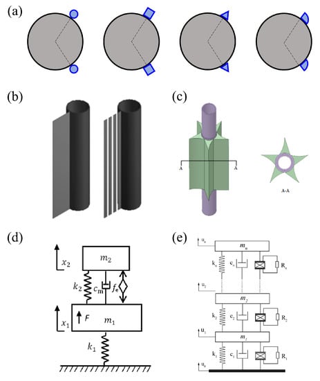
Figure 11.
Strategies to improve the power production from a vibrating cylinder undergoing FIV for energy harvesting: (a) attaching small rods (circular, square, triangular, fin-shaped); (b) attaching a splitter plate (solid and slotted) [245]; (c) attaching a free-to-rotate pentagram impeller [238]; (d) incorporating a dual-mass system [241]; and (e) utilizing a multi-degree-of-freedom system with multiple piezoelectric elements [242].
6.1. Mathematical and Numerical Modelling of FIVEH
Mathematical and numerical modellings are important tools to study FIVEH, since accurate theoretical models and CFD simulations can predict the dynamic response of the system and the power production of the energy harvester. To provide a comprehensive example of how mathematical and numerical modelling can be applied to FIVEH, we consider, specifically, a piezoelectric energy converter for this illustration.
Figure 12 depicts the main components of a simple piezoelectric energy harvester. As shown, the cylindrical rigid body connected to the free end of a cantilever beam undergoes FIV as a result of the excitation from the incident flow. This motion deforms the piezoelectric sheet bonded to the root of the cantilever beam—the deformation converts the mechanical vibration of the body to electrical energy in the interface circuit with a load resistance of R. Note that the fluid, the bluff body, and the piezoelectric transducer are considered as a single dynamical system that can be modelled using a set of governing equations—these equations can be solved to determine the vibration response and the power output of the energy harvester.
Figure 12.
Sketch of a simple piezoelectric energy harvester based on flow-induced vibration.
The semi-empirical model described in Section 3 provides the coupling of a fluid motion equation (wake oscillator) and an equation of motion for the body (mass–spring–damper system). In addition, a governing equation for the piezoelectric circuit is required to model the system. In accordance to Erturk and Inman [246], a SDOF lumped-parameter model that describes the coupled electro-mechanical system can be expressed as
If we compare these equations to the mathematical model (Equation (13)) in Section 3, the equation of motion of the structure given by Equation (39) has been modified to include the mechanical force which is modelled as being proportional to the voltage across the external electrical load resistance R with the coefficient of proportionality for the coupling to the electro-mechanical system given by . Other physical quantities, such as , , , y, and , have the same meaning as those in Equation (13). Equation (40) is the circuit equation where arises from the capacitance of the piezoelectric layer and the electro-mechanical coupling .
If the rigid body in Figure 12 is replaced with a smooth circular cylinder, the system becomes a VIV-based piezoelectric energy harvester. Dai et al. [247] developed a reduced-order model for this device by utilizing the Euler–Lagrange principle and a Galerkin discretization based on the wake-oscillator model proposed by Facchinetti et al. [27]. The governing equations are given by
Equation (41) models the motion of the free end of the piezoelectric beam where () denotes the modal coordinates of the displacement; and are the lengths of the cylinder and the substrate layer, respectively; is the displacement of the end of the cantilever beam. Equation (42) encapsulates the dynamics of the near wake behind the cylinder based on Facchinetti et al.’s wake oscillator model with an acceleration coupling term—here, and A = 1.2. Equation (43) is the governing equation for the piezoelectric circuit, similar to Equation (40). Dai et al. [247] validated their non-linear mathematical model using some experimental results and reported a very good agreement. These investigators applied this model to study the effect of the tip mass and the piezoelectric sheet length on the maximum generated voltage and harvested power of the piezoelelectri energy harvester.
The linear benchmark model [247] is a common theoretical form for the FIV piezoelectric energy harvester. A number of researchers has modified this basic form and tailored it to solve various engineering problems. For example, Hou et al. [248] introduced a non-linear magnetic force term into Equation (41) with the following form:
Here, , M and are the vacuum permeability, the magnetization intensity, and the distance between the magnets, respectively.
Rather than formulating the VIV aerodynamic force using a wake-oscillator model, Wang et al. [249] presented a new semi-empirical model for the VIV piezoelectric energy harvester using the Scanlan–Ehsan non-linear representation for the forcing term in Equation (39). This formulation was compared to some wind-tunnel data and found to yield accurate predictions. A significant benefit of this model is that it can be used not only for a smooth circular cylinder, but also for cylinders having different cross-sectional shapes and for a cylinder–attachment system.
Galloping is provoked when a square or rectangular cylinder is incorporated in the beam. For a piezoelectric energy harvester exhibiting galloping, the external excitation can be modelled using quasi-steady theory—the modelling here is similar to that for the polynomial expansion of the transverse force coefficient (see Section 3.3 for more details). While the electro-mechanical coupling term is different, the model can be formulated in a number of ways, such as: (1) using a simple SDOF mass–spring–damper system [250,251]; (2) using a distributed parameter model with Rayleigh–Ritz discretization [252]; and (3) using a Euler–Bernoulli distributed parameter model [253]. A mathematical model can also be derived for the piezoelectric energy harvester based on other types of FIV response, such as a flutter converter [253] and a wake-galloping converter [254]. As a final note, the use of a SDOF mass–spring–damper system [250,251] mentioned here involves simply using an odd-order polynomial approximation for in Equation (39) which results in
In addition to mathematical modelling (described above), numerical modelling based on CFD can be employed to predict the dynamics of the FIV piezoelectric energy harvester. To this purpose, numerical modelling can be used in several different ways to address problems related to FIVEH. Firstly, high-fidelity CFD predictions can be used to validate various theoretical models of FIVEH (e.g., the analytical and semi-empirical models mentioned above). Secondly, the distributed parameters in a semi-empirical model of FIVEH can be determined using reliable data obtained from high-fidelity numerical simulations (e.g., DNS or LES), especially when wind-tunnel experimental data are not available. Thirdly, CFD can be used to predict the detail characteristics of the flow and the power efficiency of a FIV energy harvester [255,256,257,258,259,260,261]. This is of particular importance when it is difficult and/or impossible to develop a detailed mathematical model for an energy harvester (e.g., a harvester that utilizes a bluff body having a very complex geometry). Generally, CFD simulations generate more accurate predictions than those provided by any analytical and/or semi-empirical mathematical model, frequently at only a fraction of the cost required for conducting a detailed experimental investigation. As a result, numerical modelling occupies a central role in research concerning FIVEH.
Recently, Ramirez [262] proposed a new modelling approach which couples CFD with an electro-mechanical model to obtain the flow dynamics and the electric power of multiple interacting energy harvesters. The approach advocated here is to integrate the NS equations for incompressible fluid flow with the Gauss law for the piezoelectric equations and the mass–spring–damper system for the oscillating rigid body. The proposed model uses the NS equations to make detailed predictions of the flow, rather than employing a simple (semi-empirical) wake-oscillator model, so it can generate more accurate predictions of the FIV displacement in the energy harvester.
In summary, employing reliable mathematical and numerical modelling can effectively predict the aerodynamic response of a bluff body, such as the vibration displacement, the frequency, and the lift force, as well as the power and output voltage of an energy harvester of a specified design. Moreover, these powerful mathematical and numerical tools can be used to undertake a parametric study of the influence of various aero-electro-mechanical parameters relevant to the system on the performance of the FIV energy harvester.
6.2. Machine Learning for Modelling FIVEH
Until now, traditional research methods, such as theoretical analysis (mathematical modelling), CFD simulations (numerical modelling), and wind-tunnel experiments, are still the principal approaches used to investigate FIVEH, but these approaches have some limitations. For example, a mathematical model is not always available for a complicated FIV energy harvester that has an irregular cross-sectional shape, or attached with small devices, or consists of a multi-cylinder system. On the other hand, CFD simulations and experimental investigations are time-consuming and expensive. As a consequence, machine learning approaches capable of addressing the FSI problem (see Section 5) is another efficient and economical alternative methodology that can be used to predict the dynamic response intensity and power generation capacity of a FIV energy harvester.
Some researchers employ machine learning and neural networks to wind assessment (e.g., wind speed, wind pressure) and power forecasting of a large-scale horizontal-axis wind turbine or a wind farm [263,264,265,266], which is instructional to the implementation of these artificial intelligence (AI) approaches on a FIV energy harvester. However, to the authors’ knowledge, there are very few studies that apply ML or NN in the prediction of the dynamics associated with a FIV energy harvester. Two representative works will be reviewed here in detail in order to help the reader understand and appreciate the possible and feasible application of ML to support the design of current and future energy harvesters for exploiting FIV.
Zhang et al. [267] investigated wake galloping in a piezoelectric energy harvester consisting of an upstream stationary obstacle and a downstream piezoelectric cantilever beam connected with a cuboid bluff body on the free end, as shown in Figure 13. These researchers first conducted a series of wind-tunnel experiments to study the influence of shapes and sizes of upstream obstacles, as well as the distances between the fixed and vibrating body on the wake galloping response. Subsequently, they employed three different algorithms (viz., a decision-tree regression (DTR), a random forest (RF), and gradient boosting regression trees (GBRT)) to train a machine learning model based on the large datasets collected from their experimental measurements, including multiple input signals (e.g., wind speed and geometric variables), as well as two output signals (root-mean-square voltage and the maximum displacement ). These researchers found the GBRT model with best hyperparameters optimized using a ten-fold cross-validation method can obtain the most accurate predictions of and . This example demonstrates the possibility of training a ML model with experimental data to predict the power output and vibration intensity of a wake-galloping energy harvester. The modelling logic of this novel approach is summarized in Figure 14 (left panel).
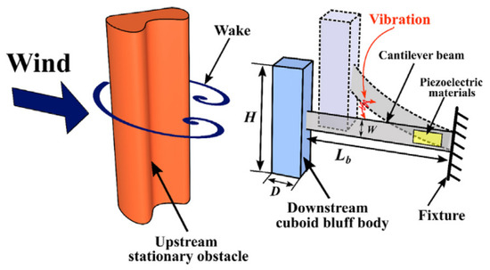
Figure 13.
Schematic of wake galloping in a piezoelectric energy harvester [267].
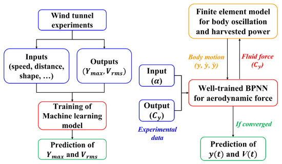
Figure 14.
Machine-learning modelling procedure for a piezoelectric energy harvester based on wake galloping [267] (left panel) and galloping [268] (right panel).
By contrast, Hu et al. [268] applied AI to model a galloping piezoelectric energy harvester in a more mathematical way. As described in Section 3.3, the most-commonly used theoretical model of galloping uses the quasi-steady assumption of the aerodynamic force. Instead of representing the external excitation by an odd-order polynomial function fitting the discretized experimental data points like others, Hu et al. [268] applied a well-trained three-layer back propagation neural network (BPNN) to establish the non-linear relationship between the force coefficient (output) and the angle of attack (input). To demonstrate the superiority of using a neural network, these researchers first replaced the polynomial expression of aerodynamic force on the right-hand side of the structural equation (Equation (45)) with the output of the trained BPNN, and combined this with the electrical circuit equation (Equation 40)) to form a BPNN SDOF model. Furthermore, the authors proposed an architecture integrating the finite-element modelling of the electro-mechanical structure with a trained BPNN of the aerodynamic force. Specifically, during each time step of simulation, the body motion calculated from the finite-element model is first passed as an input to the trained BPNN, which then predicts the aerodynamic force acting on the body at the current moment and updates the fluid force in the finite-element model in real-time. The simulation converges after an iterative process. In this case, the use of BPNN only involves the action of the fluid on the body (viz., prediction of the aerodynamic force), while the body motion and the electro-mechanical conversion are addressed by the finite-element model. A flowchart of the application logic is shown in Figure 14 (right panel).
Obviously, the above two studies use completely different AI approaches in addressing the problem of FIVEH. The first case [267] developed a non-linear black-box model for the dynamical system without knowing the particular mathematical structure or underlying physics, in which the relationship between the input and the output are obtained by training a machine learning model using a large dataset. On the other hand, the second case [268] actually lies at the intersection of machine learning and numerical modelling, in which the former is used for prediction of the aerodynamic force and the latter is responsible for calculating the motion of the bluff body and the output voltage of the energy harvester. In addition, the second application mode of AI has a more solid theoretical foundation because the flow information and the energy conversion are obtained by numerically solving the NS equations and the electro-mechanical circuit equation—in this sense, it is more useful and practical when there is a lack of training data.
In summary, AI approaches applied to the FIV energy harvesting is nascent, but as these new techniques mature and become more widespread, they could certainly aid in the design of FIV energy harvesting systems. Some of the previously mentioned PINN techniques for flow field reconstruction in Section 5 could also be applied to in situ tuning and control of a FIV energy harvester. By allowing for accelerated and more accurate simulations of FIV devices, the design process will be better informed.
7. Outlook
Flow-induced vibration of a bluff body is a classical FSI problem with deep theoretical significance and practical value. The objective of this comprehensive survey is to provide a systematic overview on the current modelling approaches for FIV—a full spectrum of approaches is reviewed including mathematical modelling, numerical simulation/modelling based on CFD and application of machine learning. These approaches are illustrated through an application to a real-world problem—design of a FIV energy harvester. Each modelling approach has its own strengths and weaknesses. In this section, we consider some of the outstanding challenges (future issues) that remain to be addressed and summarize some directions for future work and perspectives for the modelling of FIV phenomena.
7.1. Future Issues
- (1)
- Mathematical modelling.
- Mathematical modelling plays an indispensable role in our understanding of the underlying physics of the FIV phenomenon. However, formulating an accurate mathematical model for a highly non-linear dynamical system, such as FIV phenomena is highly challenging. The mathematical models proposed to date based on experimental data and/or engineering experience are not purely analytical models derived from first principles using a comprehensive theory and, as a result, these models have a limited range of applicability. Is it possible to develop a more complete theory of various aspects of FIV phenomena that will allow the formulation of more general analytical models?
- Most theoretical models for FIV, whether a coupled wake-oscillator model or single-degree-of-freedom model, are semi-empirical in nature—implying that the model has unknown parameters whose values need to be determined (fitted) to available experimental data. As a result, these models tend to have a very limited range of applicability (viz., a model that has been developed for VIV for a particular bluff body shape cannot be used for VIV for another body shape or for galloping for the same body shape without changing either the structure of the model and/or re-fitting the free parameters that define the model). More specifically, the need for reformulating the structure of terms and/or inclusion of new terms in the model along with a re-fitting of the free coefficients using available experimental data need to be conducted for new scenarios.
- Most of the current mathematical models for FIV phenomena have been developed for VIV, which can also include galloping behavior in the formulation through use of the quasi-steady assumption—this usually involves inclusion of an odd-order polynomial approximation of the aerodynamic force responsible for galloping in the mathematical model. Although some other methods (e.g., neural network mappings) have been proposed to improve the curve fitting accuracy of the forcing term responsible for galloping, it is stressed that the quasi-steady assumption has inherent limitations and is applicable only under certain conditions.
- (2)
- Numerical modelling.
- Owing to its moderate computational cost, RANS modelling will remain the workhorse of CFD applications to engineering and industrial FIV problems of practical relevance into the foreseeable future. The essential element for the successful use of RANS modelling is formulation of turbulence closure models. Is it possible to simulate FIV for these engineering and industrial applications using lower-fidelity numerical models such as unsteady RANS?
- Even so, for FIV problems that require greater accuracy or detailed information on the spatial and temporal fluctuations of the flow field, hybrid methods may be the numerical tool of choice (at least in the near future) given that these methods are not as computationally prohibitive as either LES or DNS. Hybrid methods represent the amalgamation of closure modelling with eddy-resolving simulation. The key question here is what blending and/or interpolation functions should be used in hybrid methods to give the best prediction of FIV phenomena?
- (3)
- Machine learning technique.
- In machine learning, the availability of large public datasets has spurred rapid progress in computer vision, speech recognition, and other applications. Many sophisticated machine learning techniques (including those for numerical simulation of turbulent flows) require large datasets consisting of high-quality information. Perhaps the biggest challenge for machine learning techniques within FIV simulation is the lack of availability of data. Every investigator that applies a state-of-the-art machine learning method to FIV simulation must generate their own dataset. Currently, it is impossible to benchmark various machine learning techniques, such as PINN or augmented RANS modelling as applied to FIV, because there exists no suitable public dataset for this purpose.
- Aside from the lack of available data, there are major physics-based challenges for applying machine learning technique to FIV simulation. Changes in the Reynolds number, in the freestream turbulence, in vibration parameters, and in the body shape all greatly affect the FIV response. Even without incorporating machine learning techniques, traditional physics-based numerical methods, such as RANS and LES, often struggle to reproduce the complicated interactions within FIV. When applying a machine learning technique for FIV, the design of the training dataset will be of utmost importance. Generalizability issues within machine learning greatly affect the model’s ability to perform outside of the parameters given in the training dataset. For example, a model trained at Re = 2000 may produce erroneous results at Re = 30,000, because transitional turbulence regions in the former case become fully turbulent in the latter case [269]. These small changes in turbulence can have large effects on the vibration response. Therefore, the training dataset should be designed to incorporate a wide variety of FIV parameters, so that the model can perform well for a variety of test cases. The issue of generalizability within machine learning augmented turbulence modelling is currently under investigation. Machine learning techniques may be better suited to provide accelerated and higher-accuracy simulation results within a known range of parameters, rather than attempting to uncover new physics (for example, at a higher-Reynolds number than any of the cases included in the training dataset).
- While several PINN techniques have been developed and applied to the unsteady FIV problem, RANS-based machine learning techniques for unsteady cases are still in development. The overwhelming majority of machine learning augmented RANS investigations use a steady state flow for training and testing. Some techniques within augmented RANS (e.g., iterative methods) are more suited for unsteady flows, but have not been rigorously tested. Therefore, another key issue is the ability of augmented turbulence models to be used for transient cases. Machine learning augmented LES closures are more immediately applicable for unsteady flow simulation due to the nature of LES. However, the suitability of these closure for the FIV problem is yet to be demonstrated.
7.2. Future Work and Perspectives
In spite of important advances, much remains to be done with respect to research concerning the modelling and prediction of the myriad of physical processes underlying various FIV phenomena—there is much future work to be done. In light of the challenges in current FIV modelling efforts identified in Section 7.1, we summarize directions for future work.
- With respect to the mathematical modelling of FIV phenomena, the development of a general theory for one or more aspects of FIV phenomena from first principles and the comprehensive analysis following from the application of such a general theory is a worthwhile (albeit extremely difficult) avenue of investigation.
- To allow mathematical models for FIV phenomena to have greater flexibility/generality (and lacking a general theory for FIV at present), research into the application of improved optimization methods for determination of model parameters along with an uncertainty quantification of the prediction provided by such models would be extremely beneficial.
- Work on the development of an improved mathematical representation for the inclusion of galloping in mathematical models for FIV could potentially improve significantly the prediction accuracy of the current generation of models for a bluff body experiencing either pure galloping or a combined FIV that includes galloping.
- More work needs to be done to improve the predictive accuracy of low-fidelity numerical methodologies, such as unsteady RANS modelling for routine application to FIV problems of industrial relevance. Schemes to provide improved closure models for addressing the FIV problem need to be developed. From this perspective, the application of data-driven approaches using ML (e.g., neural nets, gradient boosting machines [270]) or inverse modelling (e.g., Bayesian optimization [271], likelihood-free inference [272]) can be used to design application specific closure models for FIV phenomena.
- More effort needs to be focused on the proper application of hybrid methods to the prediction of FIV phenomena. To this purpose, more research should be conducted on the appropriate selection of the mode of computation (whether RANS modelling or eddy-resolving simulation) that is specifically tailored to address the peculiarities of FIV phenomena (e.g., development of a specific hybrid blending or interpolation function that more intelligently selects whether RANS or eddy-resolving simulation should be used in various regions of the FIV flows).
- Methods of machine learning can be applied potentially to provided improved closure models for numerical simulation of FIV phenomena. However, for this to occur, a considerable effort should be made to obtain high-quality FIV datasets from high-fidelity numerical simulation (DNS and/or LES). The authors strongly encourage the future publication of public-domain FIV datasets that can be used for bench marking machine learning techniques.
- Work should be undertaken to better understand the synergy in mathematical, numerical, and machine learning techniques for the modelling of FIV phenomena (and, more specifically, on how to exploit this synergy to advance future modelling efforts in this field of endeavor). For example, high-fidelity numerical simulation methodologies (DNS and/or LES) provide the data for machine learning algorithms that can potentially lead to improved closure models for low-fidelity RANS models. The predictions obtained from these models provide the information required to obtain deeper insights and a better understanding of FIV phenomenology—this better understanding can potentially lead to the development of improved and more principled and general mathematical models of FIV phenomena.
The key takeaway of this review is that modelling is arguably the most important tool for investigation of various aspects of FIV phenomena. Advances in the modelling of FIV phenomena will undoubtedly impact a number of engineering and industrial applications of practical real-world relevance. A deeper understanding of FIV phenomena will allow engineers to design potentially significantly improved fluid kinetic energy harvesting devices (viz., enhance the energy harvesting efficiency of such devices). However, this application will require development of a system-of-systems modelling approach involving coupling models of FIV, electromechanics, and complex interface circuits. Alternatively, modelling advances in FIV will lead to a better understanding of fatigue failure arising from vibration in structures exposed to high energy fluid flow (e.g., transmission lines critical to modern electricity generation infrastructure, fuel rod assembly in conventional or small modular nuclear reactors and implications for nuclear safety, risers for deep water applications, such as oil and gas production). An under-explored area of research in FIV is multi-physics coupling in the simulation. For example, transmission lines in cold climates during winter storms are subject to icing as well as to wind-induced (aeolian) vibration that can cause outages—how the vibration response of the transmission line is altered with ice accretion has not been studied to the authors’ knowledge.
Author Contributions
Conceptualization, F.-S.L. and E.Y.; methodology, Y.W., Z.C. and R.M.; software, Y.W., Z.C.; validation, Y.W., Z.C., R.M., F.-S.L. and E.Y.; formal analysis, Y.W.; investigation, Y.W., Z.C., R.M., F.-S.L. and E.Y.; resources, F.-S.L.; data curation, Y.W. and Z.C.; writing—original draft preparation, Y.W., Z.C. and R.M.; writing—review and editing, E.Y. and F.-S.L.; visualization, Y.W. and Z.C.; supervision, F.-S.L. and E.Y.; project administration, F.-S.L. and E.Y.; funding acquisition, F.-S.L. All authors have read and agreed to the published version of the manuscript.
Funding
This research was funded by the Natural Sciences and Engineering Research Council of Canada (NSERC) Discovery Grants program Grant Nos. 50503-10234.
Data Availability Statement
Not applicable.
Conflicts of Interest
The authors declare no conflict of interest.
Abbreviations
The following abbreviations are used in this manuscript:
| AI | Artificial Intelligence |
| ALE | Arbitrary Lagrangian–Eulerian |
| AOA | Angle of Attack |
| ARX | Autoregressive with Exogenous Input |
| BPNN | Back Propagation Neural Network |
| BPOD | Balanced POD |
| CAE | Computer-Aided Engineering |
| CFD | Computational Fluids Dynamics |
| CNN | Convolutional Neural Network |
| CRAN | Convolutional Recurrent Autoencoder Network |
| DDES | Delayed Detached-Eddy Simulation |
| DES | Detached-Eddy Simulation |
| DEIM | Discrete Empirical Interpolation Method |
| DMD | Dynamic Mode Decomposition |
| DNN | Deep Neural Network |
| DNS | Direct Numerical Simulation |
| DSD/SST | Deforming-Spatial-Domain/Stabilized Space-Time |
| DTR | Decision-Tree Regression |
| DVM | Discrete Vortex Method |
| EB | embedded boundary |
| ERA | Eigensystem Realization Algorithm |
| EVM | Entropy–Viscosity Method |
| FD | Fictitious Domain |
| FDM | Finite Differencing Method |
| FEM | Finite Element Method |
| FIV | Flow-Induced Vibration |
| FIVEH | Flow-Induced Vibration Energy Harvesting |
| FOM | Full-Order Model |
| FSI | Flow-Structure Interaction |
| FVM | Finite Volume Method |
| GBRT | Gradient Boosting Regression Trees |
| IBM | Immersed Boundary Method |
| LBM | Lattice-Boltzmann Method |
| LES | Large-Eddy Simulation |
| LSA | Linear Stability Analysis |
| LSTM | Long Short-Term Memory |
| ML | Machine Learning |
| MTS | Multiple Time Scales |
| NS | Navier–Stokes |
| NS-PINN | Navier–Stokes equations-based PINN |
| ODE | Ordinary Differential Equation |
| PDE | Partial Differential Equation |
| PG-FEM | Petrov–Galerkin Finite Element Method |
| PINN | Physics-Informed Neural Networks |
| PNS-PINN | Parameterized Navier–Stokes equations-based PINN |
| POD | Proper Orthogonal Decomposition |
| PTC | Passive Turbulence Control |
| QS | Quasi-Steady |
| RANS | Reynolds-averaged Navier–Stokes |
| RBFNN | Radial Basis Function Neural Network |
| RF | Random Forest |
| RNN | Recurrent Neural Network |
| ROM | Reduced-Order Model |
| SA | Spalart–Allmaras |
| SDOF | Single Degree-Of-Freedom |
| SEM | Spectral Elements Method |
| SGS | Sub-grid Scale |
| SM | Smagorinsky |
| SPOD | Spectral POD |
| SST | Shear Stress Transport |
| SST-FEM | Stabilized Space–Time FEM |
| SVD | Singular Value Decomposition |
| TBNN | Tensor Basis Neural Network |
| VIV | Vortex-Induced Vibration |
| WALE | Wall-Adapting Local-Eddy |
| mPOD | Multiscale POD |
| 1DOF | One-Degree-Of-Freedom |
| 2DOF | Two-Degree-Of-Freedom |
| 2D | Two-Dimensional |
| 3D | Three-Dimensional |
References
- Nakamura, T.; Kaneko, S.; Inada, F.; Kato, M.; Ishihara, K.; Nishihara, T.; Mureithi, N.W.; Langthjem, M.A. Flow-Induced Vibrations: Classifications and Lessons from Practical Experiences; Butterworth-Heinemann: Portsmouth, NH, USA, 2013. [Google Scholar]
- Parkinson, G. Phenomena and modelling of flow-induced vibrations of bluff bodies. Prog. Aerosp. Sci. 1989, 26, 169–224. [Google Scholar] [CrossRef]
- Brunton, S.L.; Noack, B.R.; Koumoutsakos, P. Machine learning for fluid mechanics. Annu. Rev. Fluid Mech. 2020, 52, 477–508. [Google Scholar] [CrossRef]
- Kutz, J.N. Deep learning in fluid dynamics. J. Fluid Mech. 2017, 814, 1–4. [Google Scholar] [CrossRef]
- Usman, A.; Rafiq, M.; Saeed, M.; Nauman, A.; Almqvist, A.; Liwicki, M. Machine learning computational fluid dynamics. In Proceedings of the IEEE 2021 Swedish Artificial Intelligence Society Workshop (SAIS), Stockholm, Sweden, 14–15 June 2021; pp. 1–4. [Google Scholar]
- Ma, X.; Zhou, S. A review of flow-induced vibration energy harvesters. Energy Convers. Manag. 2022, 254, 115223. [Google Scholar] [CrossRef]
- Wang, J.; Geng, L.; Ding, L.; Zhu, H.; Yurchenko, D. The state-of-the-art review on energy harvesting from flow-induced vibrations. Appl. Energy 2020, 267, 114902. [Google Scholar] [CrossRef]
- Lv, Y.; Sun, L.; Bernitsas, M.M.; Sun, H. A comprehensive review of nonlinear oscillators in hydrokinetic energy harnessing using flow-induced vibrations. Renew. Sustain. Energy Rev. 2021, 150, 111388. [Google Scholar] [CrossRef]
- Blevins, R.D. Flow-Induced Vibration; Van Nostrand Reinhold Company: New York, NY, USA, 1977. [Google Scholar]
- Rostami, A.B.; Armandei, M. Renewable energy harvesting by vortex-induced motions: Review and benchmarking of technologies. Renew. Sustain. Energy Rev. 2017, 70, 193–214. [Google Scholar] [CrossRef]
- Tamura, Y. Mathematical models for understanding phenomena: Vortex-induced vibrations. Jpn. Archit. Rev. 2020, 3, 398–422. [Google Scholar] [CrossRef]
- Su, Y.; Di, J.; Li, S.; Jian, B.; Liu, J. Buffeting response prediction of long-span bridges based on different wind tunnel test techniques. Appl. Sci. 2022, 12, 3171. [Google Scholar] [CrossRef]
- Luongo, A.; Piccardo, G. Linear instability mechanisms for coupled translational galloping. J. Sound Vib. 2005, 288, 1027–1047. [Google Scholar] [CrossRef]
- Gabbai, R.D.; Benaroya, H. An overview of modeling and experiments of vortex-induced vibration of circular cylinders. J. Sound Vib. 2005, 282, 575–616. [Google Scholar] [CrossRef]
- Païdoussis, M.P.; Price, S.J.; De Langre, E. Fluid-Structure Interactions: Cross-Flow-Induced Instabilities; Cambridge University Press: Cambridge, UK, 2010. [Google Scholar]
- Rayleigh, J.W.S.B. The Theory of Sound; Macmillan: New York, NY, USA, 1896; Volume 2. [Google Scholar]
- van der Pol, B.; van der Mark, J. LXXII. The heartbeat considered as a relaxation oscillation, and an electrical model of the heart. Lond. Edinb. Dublin Philos. Mag. J. Sci. 1928, 6, 763–775. [Google Scholar] [CrossRef]
- Goswami, U. Toward an interactive analogy model of reading development: Decoding vowel graphemes in beginning reading. J. Exp. Child Psychol. 1993, 56, 443–475. [Google Scholar] [CrossRef]
- Bishop, R.E.D.; Hassan, A. The lift and drag forces on a circular cylinder oscillating in a flowing fluid. Proc. R. Soc. Lond. Ser. Math. Phys. Sci. 1964, 277, 51–75. [Google Scholar]
- Hartlen, R.T.; Currie, I.G. Lift-oscillator model of vortex-induced vibration. J. Eng. Mech. Div. 1970, 96, 577–591. [Google Scholar] [CrossRef]
- Skop, R.; Griffin, O. A model for the vortex-excited resonant response of bluff cylinders. J. Sound Vib. 1973, 27, 225–233. [Google Scholar] [CrossRef]
- Griffin, O.; Skop, R.; Koopmann, G. The vortex-excited resonant vibrations of circular cylinders. J. Sound Vib. 1973, 31, 235–IN3. [Google Scholar] [CrossRef]
- Landl, R. A mathematical model for vortex-excited vibrations of bluff bodies. J. Sound Vib. 1975, 42, 219–234. [Google Scholar] [CrossRef]
- Skop, R.; Griffin, O. On a theory for the vortex-excited oscillations of flexible cylindrical structures. J. Sound Vib. 1975, 41, 263–274. [Google Scholar] [CrossRef]
- Skop, R.; Balasubramanian, S. A new twist on an old model for vortex-excited vibrations. J. Fluids Struct. 1997, 11, 395–412. [Google Scholar] [CrossRef]
- Skop, R.; Luo, G. An inverse-direct method for predicting the vortex-induced vibrations of cylinders in uniform and nonuniform flows. J. Fluids Struct. 2001, 15, 867–884. [Google Scholar] [CrossRef]
- Facchinetti, M.L.; De Langre, E.; Biolley, F. Coupling of structure and wake oscillators in vortex-induced vibrations. J. Fluids Struct. 2004, 19, 123–140. [Google Scholar] [CrossRef]
- Ogink, R.; Metrikine, A. A wake oscillator with frequency dependent coupling for the modeling of vortex-induced vibration. J. Sound Vib. 2010, 329, 5452–5473. [Google Scholar] [CrossRef]
- Furnes, G.K.; Sørensen, K. Flow induced vibrations modeled by coupled non-linear oscillators. In Proceedings of the Seventeenth International Offshore and Polar Engineering Conference, Lisbon, Portugal, 1–6 July 2007; OnePetro: Richardson, TX, USA, 2007. [Google Scholar]
- Ge, F.; Long, X.; Wang, L.; Hong, Y. Flow-induced vibrations of long circular cylinders modeled by coupled nonlinear oscillators. Sci. China Ser. Phys. Mech. Astron. 2009, 52, 1086–1093. [Google Scholar] [CrossRef]
- Srinil, N.; Zanganeh, H. Modelling of coupled cross-flow/in-line vortex-induced vibrations using double Duffing and van der Pol oscillators. Ocean Eng. 2012, 53, 83–97. [Google Scholar] [CrossRef]
- Bai, X.; Qin, W. Using vortex strength wake oscillator in modelling of vortex induced vibrations in two degrees of freedom. Eur. J. Mech. B Fluids 2014, 48, 165–173. [Google Scholar] [CrossRef]
- Postnikov, A.; Pavlovskaia, E.; Wiercigroch, M. 2DOF CFD calibrated wake oscillator model to investigate vortex-induced vibrations. Int. J. Mech. Sci. 2017, 127, 176–190. [Google Scholar] [CrossRef]
- Birkhoff, G. Formation of vortex streets. J. Appl. Phys. 1953, 24, 98–103. [Google Scholar] [CrossRef]
- Kutta, W. Auftriebskräfte in strömenden Flüssigkeiten. Illus. Aeronaut. Mitteilung. 1902, 6, 133–135. [Google Scholar]
- Joukowsky, N. Über die konturen der Tragflächen der Drachenflieger. Z. Flugtech. Mot. 1910, 1, 281–285. [Google Scholar]
- Funakawa, M. Excitation mechanism of elastically supported circular cylinder in the flow. Bull. Jpn. Soc. Mech. Eng. 1970, 36, 303–312. [Google Scholar]
- Tamura, Y. Vortex induced vibration of circular cylinder (Part I Wake oscillator model). Trans. Archit. Inst. Jpn. 1978, 266, 87–95. [Google Scholar] [CrossRef]
- Tamura, Y.; Matsui, G. Wind Engineering, Proceedings of the 5th International Conference on Wind Engineering, Fort Collins, CO, USA, 8–13 July 1979; Cermak, J.E., Ed.; Pergamon Press Ltd.: Amsterdam, The Netherlands, 1979; Volume 266, pp. 1085–1094. [Google Scholar]
- Tamura, Y.; Amano, A. Mathematical model for vortex-induced oscillations of continuous systems with circular cross section. J. Wind. Eng. Ind. Aerodyn. 1983, 14, 431–442. [Google Scholar] [CrossRef]
- Iwan, W.; Blevins, R. A model for vortex induced oscillation of structures. J. Appl. Mech. 1974, 41, 581–586. [Google Scholar] [CrossRef]
- Krenk, S.; Nielsen, S.R. Energy balanced double oscillator model for vortex-induced vibrations. J. Eng. Mech. 1999, 125, 263–271. [Google Scholar] [CrossRef]
- Scanlan, R.H. State-of-the-Art Methods For Calculating Flutter, Vortex-Induced, and Buffeting Response of Bridge Structures; Technical Report No. FHWA/RD-80-050; Federal Highway Administration: Washington, DC, USA, 1981. [Google Scholar]
- Simiu, E.; Scanlan, R. Wind Effects on Structures, 2nd ed.; John Wiley and Sons: Hoboken, NJ, USA, 1986. [Google Scholar]
- Ehsan, F.; Scanlan, R.H.; Bosch, H.R. Modeling spanwise correlation effects in the vortex-induced response of flexible bridges. J. Wind. Eng. Ind. Aerodyn. 1990, 36, 1105–1114. [Google Scholar] [CrossRef]
- Billah, K.Y.R. A Study of Vortex-Induced Vibration. Ph.D. Thesis, Princeton University, Princeton, NJ, USA, 1989. [Google Scholar]
- Goswami, I.; Scanlan, R.H.; Jones, N.P. Vortex-induced vibration of circular cylinders. II: New model. J. Eng. Mech. 1993, 119, 2288–2302. [Google Scholar] [CrossRef]
- Sarpkaya, T. Fluid forces on oscillating cylinders. J. Waterw. Port, Coast. Ocean. Div. 1978, 104, 275–290. [Google Scholar] [CrossRef]
- Staubli, T. Calculation of the vibration of an elastically mounted cylinder using experimental data from forced oscillation. J. Fluids Eng. 1983, 105, 225–229. [Google Scholar] [CrossRef]
- Stäubli, M.; Bircher, J.; Galeazzi, R.; Remund, H.; Studer, H. Serum concentrations of amiodarone during long term therapy. Relation to dose, efficacy and toxicity. Eur. J. Clin. Pharmacol. 1983, 24, 485–494. [Google Scholar] [CrossRef]
- Griffin, O.; Koopmann, G. The vortex-excited lift and reaction forces on resonantly vibrating cylinders. J. Sound Vib. 1977, 54, 435–448. [Google Scholar] [CrossRef]
- Feng, C. The Measurement of Vortex Induced Effect in Flow Past Stationary and Oscillating Circular and D-Section Cylinders. Master’s Thesis, University of British Columbia, Vancouver, BC, Canada, 1968. [Google Scholar]
- Parkinson, G.; Sullivan, P. Galloping response of towers. J. Wind. Eng. Ind. Aerodyn. 1979, 4, 253–260. [Google Scholar] [CrossRef]
- den Hartog, J. Transmission line vibration due to sleet. Trans. Am. Inst. Electr. Eng. 1932, 51, 1074–1076. [Google Scholar] [CrossRef]
- Meseguer Ruiz, J.; Sanz Andres, A.P.; Alonso Rodrigo, G. Determination of maximum mechanical energy efficiency in energy galloping systems. J. Eng. Mech. 2015, 141, 1–8. [Google Scholar] [CrossRef]
- Alonso, G.; Meseguer, J.; Pérez-Grande, I. Galloping stability of triangular cross-sectional bodies: A systematic approach. J. Wind. Eng. Ind. Aerodyn. 2007, 95, 928–940. [Google Scholar] [CrossRef]
- Simiu, E.; Yeo, D. Wind Effects on Structures: Modern Structural Design for Wind; John Wiley & Sons: Hoboken, NJ, USA, 2019. [Google Scholar]
- Parkinson, G.; Brooks, N. On the aeroelastic instability of bluff cylinders. J. Appl. Mech. 1961, 28, 252–258. [Google Scholar] [CrossRef]
- Parkinson, G.; Smith, J. The square prism as an aeroelastic non-linear oscillator. Q. J. Mech. Appl. Math. 1964, 17, 225–239. [Google Scholar] [CrossRef]
- Luo, S.; Chew, Y.; Ng, Y. Hysteresis phenomenon in the galloping oscillation of a square cylinder. J. Fluids Struct. 2003, 18, 103–118. [Google Scholar] [CrossRef]
- Ng, Y.; Luo, S.; Chew, Y. On using high-order polynomial curve fits in the quasi-steady theory for square-cylinder galloping. J. Fluids Struct. 2005, 20, 141–146. [Google Scholar] [CrossRef]
- Barrero-Gil, A.; Sanz-Andres, A.; Roura, M. Transverse galloping at low Reynolds numbers. J. Fluids Struct. 2009, 25, 1236–1242. [Google Scholar] [CrossRef]
- Joly, A.; Etienne, S.; Pelletier, D. Galloping of square cylinders in cross-flow at low Reynolds numbers. J. Fluids Struct. 2012, 28, 232–243. [Google Scholar] [CrossRef]
- Piccardo, G.; Pagnini, L.C.; Tubino, F. Some research perspectives in galloping phenomena: Critical conditions and post-critical behavior. Contin. Mech. Thermodyn. 2015, 27, 261–285. [Google Scholar] [CrossRef]
- Bearman, P.; Gartshore, I.; Maull, D.; Parkinson, G. Experiments on flow-induced vibration of a square-section cylinder. J. Fluids Struct. 1987, 1, 19–34. [Google Scholar] [CrossRef]
- Norberg, C. Flow around rectangular cylinders: Pressure forces and wake frequencies. J. Wind. Eng. Ind. Aerodyn. 1993, 49, 187–196. [Google Scholar] [CrossRef]
- Desai, Y.; Shah, A.; Popplewell, N. Galloping analysis for two-degree-of-freedom oscillator. J. Eng. Mech. 1990, 116, 2583–2602. [Google Scholar] [CrossRef]
- Jones, K.F. Coupled vertical and horizontal galloping. J. Eng. Mech. 1992, 118, 92–107. [Google Scholar] [CrossRef]
- He, M.; Macdonald, J.H. An analytical solution for the galloping stability of a 3 degree-of-freedom system based on quasi-steady theory. J. Fluids Struct. 2016, 60, 23–36. [Google Scholar] [CrossRef]
- He, M.; Macdonald, J. 3DOF galloping analysis based on quasi-steady theory with reference to the aerodynamic stiffness coupling. In Proceedings of the 7th European and African Conference on Wind Engineering, Liege, Belgium, 4–7 July 2017. [Google Scholar]
- Parkinson, G.; Wawzonek, M. Some considerations of combined effects of galloping and vortex resonance. J. Wind. Eng. Ind. Aerodyn. 1981, 8, 135–143. [Google Scholar] [CrossRef]
- Parkinson, G.; Bouclin, D. Hydroelastic oscillations of square cylinders. In Proceedings of the International Research Seminar on Safety of Structures under Dynamic Loading, Trondheim, Norway, 25–30 June 1977. [Google Scholar]
- Corless, R.M.; Parkinson, G. A model of the combined effects of vortex-induced oscillation and galloping. J. Fluids Struct. 1988, 2, 203–220. [Google Scholar] [CrossRef]
- Han, P.; Hémon, P.; Pan, G.; de Langre, E. Nonlinear modeling of combined galloping and vortex-induced vibration of square sections under flow. Nonlinear Dyn. 2021, 103, 3113–3125. [Google Scholar] [CrossRef]
- Tamura, Y.; Shimada, K. A mathematical model for the transverse oscillations of square cylinders. In Proceedings of the International Conference on Flow Induced Vibrations, Bowness-Windermere, UK, 12–14 May 1987; pp. 12–14. [Google Scholar]
- Mannini, C.; Massai, T.; Marra, A.M.; Bartoli, G. Modelling the interaction of VIV and galloping for rectangular cylinders. In Proceedings of the 14th International Conference on Wind Engineering, Porto Alegre, Brazil, 21–26 June 2015; pp. 1–20. [Google Scholar]
- Mannini, C.; Massai, T.; Marra, A.M. Modeling the interference of vortex-induced vibration and galloping for a slender rectangular prism. J. Sound Vib. 2018, 419, 493–509. [Google Scholar] [CrossRef]
- Mannini, C. Incorporation of turbulence in a nonlinear wake-oscillator model for the prediction of unsteady galloping response. J. Wind. Eng. Ind. Aerodyn. 2020, 200, 104141. [Google Scholar] [CrossRef]
- Chen, C.; Mannini, C.; Bartoli, G.; Thiele, K. Wake oscillator modeling the combined instability of vortex induced vibration and galloping for a 2: 1 rectangular cylinder. J. Fluids Struct. 2022, 110, 103530. [Google Scholar] [CrossRef]
- Funakawa, M. The vibration of a cylinder caused by wake force in a flow. Bull. JSME 1969, 12, 1003–1010. [Google Scholar] [CrossRef][Green Version]
- ANSYS Homepage. Available online: http:www.ansys.com (accessed on 30 August 2022).
- Siemens PLM STAR-CCM+ Homepage. Available online: https://mdx.plm.automation.siemens.com/star-ccm-plus (accessed on 30 August 2022).
- OpenFOAM Project Homepage. Available online: http://www.openfoam.org (accessed on 30 August 2022).
- Selvam, R.P. Computational Fluid Dynamics for Wind Engineering; John Wiley & Sons: Hoboken, NJ, USA, 2022. [Google Scholar]
- Zhao, M.; Cheng, L. Vortex-induced vibration of a circular cylinder of finite length. Phys. Fluids 2014, 26, 2548. [Google Scholar] [CrossRef]
- Hou, G.; Wang, J.; Layton, A. Numerical methods for fluid-structure interaction—A review. Commun. Comput. Phys. 2012, 12, 337–377. [Google Scholar] [CrossRef]
- Singh, S.; Mittal, S. Vortex-induced oscillations at low Reynolds numbers: Hysteresis and vortex-shedding modes. J. Fluids Struct. 2005, 20, 1085–1104. [Google Scholar] [CrossRef]
- Mittal, S. Free vibrations of a cylinder: 3-D computations at Re = 1000. J. Fluids Struct. 2013, 41, 109–118. [Google Scholar]
- Alauzet, F. A changing-topology moving mesh technique for large displacements. Eng. Comput. 2014, 30, 175–200. [Google Scholar] [CrossRef]
- Mittal, S.; Kumar, V. Finite element study of vortex-induced cross-flow and in-line oscillations of a circular cylinder at low Reynolds numbers. Int. J. Numer. Methods Fluids 1999, 31, 1087–1120. [Google Scholar] [CrossRef]
- Longatte, E.; Bendjeddou, Z.; Souli, M. Application of arbitrary Lagrange Euler formulations to flow-induced vibration problems. J. Press. Vessel Technol. 2003, 125, 411–417. [Google Scholar] [CrossRef]
- Zhao, M.; Cheng, L. Numerical simulation of two-degree-of-freedom vortex-induced vibration of a circular cylinder close to a plane boundary. J. Fluids Struct. 2011, 27, 1097–1110. [Google Scholar] [CrossRef]
- Zhao, M.; Cheng, L. Numerical simulation of vortex-induced vibration of four circular cylinders in a square configuration. J. Fluids Struct. 2012, 31, 125–140. [Google Scholar] [CrossRef]
- Zhao, M. Flow induced vibration of two rigidly coupled circular cylinders in tandem and side-by-side arrangements at a low Reynolds number of 150. Phys. Fluids 2013, 25, 123601. [Google Scholar] [CrossRef]
- Zhao, M.; Cheng, L.; Zhou, T. Numerical simulation of vortex-induced vibration of a square cylinder at a low Reynolds number. Phys. Fluids 2013, 25, 023603. [Google Scholar] [CrossRef]
- Zhao, M.; Cheng, L.; An, H.; Lu, L. Three-dimensional numerical simulation of vortex-induced vibration of an elastically mounted rigid circular cylinder in steady current. J. Fluids Struct. 2014, 50, 292–311. [Google Scholar] [CrossRef]
- Zhao, M.; Cheng, L.; An, H.; Tong, F. Flow and flow-induced vibration of a square array of cylinders in steady currents. Fluid Dyn. Res. 2015, 47, 045505. [Google Scholar] [CrossRef]
- Griffith, B.E.; Patankar, N.A. Immersed methods for fluid-structure interaction. Annu. Rev. Fluid Mech. 2020, 52, 421. [Google Scholar] [CrossRef]
- Chen, W.; Ji, C.; Xu, W.; Liu, S.; Campbell, J. Response and wake patterns of two side-by-side elastically supported circular cylinders in uniform laminar cross-flow. J. Fluids Struct. 2015, 55, 218–236. [Google Scholar] [CrossRef]
- Peskin, C.S. Flow Patterns Around Heart Valves: A Digital Computer Method for Solving the Equations of Motion; Yeshiva University: Manhattan, NY, USA, 1972. [Google Scholar]
- Ji, C.; Xiao, Z.; Wang, Y.; Wang, H. Numerical investigation on vortex-induced vibration of an elastically mounted circular cylinder at low Reynolds number using the fictitious domain method. Int. J. Comput. Fluid Dyn. 2011, 25, 207–221. [Google Scholar] [CrossRef]
- Löhner, R.; Baum, J.D.; Mestreau, E.; Sharov, D.; Charman, C.; Pelessone, D. Adaptive embedded unstructured grid methods. Int. J. Numer. Methods Eng. 2004, 60, 641–660. [Google Scholar] [CrossRef]
- Gonzalez Cornejo, F.A.; Cruchaga, M.A.; Celentano, D.J. Modelling low Reynolds number vortex-induced vibration problems with a fixed mesh fluid-solid interaction formulation. Phys. Fluids 2017, 29, 113601. [Google Scholar] [CrossRef]
- Wall, W.A.; Gerstenberger, A.; Gamnitzer, P.; Förster, C.; Ramm, E. Large deformation fluid-structure interaction–Advances in ALE methods and new fixed grid approaches. In Fluid-Structure Interaction; Springer: Berlin/Heidelberg, Germany, 2006; pp. 195–232. [Google Scholar]
- Al-Jamal, H.; Dalton, C. Vortex induced vibrations using large-eddy simulation at a moderate Reynolds number. J. Fluids Struct. 2004, 19, 73–92. [Google Scholar] [CrossRef]
- Carmo, B.S.; Sherwin, S.J.; Bearman, P.W.; Willden, R. Flow-induced vibration of a circular cylinder subjected to wake interference at low Reynolds number. J. Fluids Struct. 2011, 27, 503–522. [Google Scholar] [CrossRef]
- Williamson, C.H.; Roshko, A. Vortex formation in the wake of an oscillating cylinder. J. Fluids Struct. 1988, 2, 355–381. [Google Scholar] [CrossRef]
- Barkley, D.; Henderson, R.D. Three-dimensional Floquet stability analysis of the wake of a circular cylinder. J. Fluid Mech. 1996, 322, 215–241. [Google Scholar] [CrossRef]
- Jiang, H.; Cheng, L.; An, H. Three-dimensional wake transition of a square cylinder. J. Fluid Mech. 2018, 842, 102–127. [Google Scholar] [CrossRef]
- Ryan, K.; Thompson, M.C.; Hourigan, K. Three-dimensional transition in the wake of bluff elongated cylinders. J. Fluid Mech. 2005, 538, 1–29. [Google Scholar] [CrossRef]
- Leontini, J.S.; Jacono, D.L.; Thompson, M.C. Stability analysis of the elliptic cylinder wake. J. Fluid Mech. 2015, 763, 302–321. [Google Scholar] [CrossRef]
- Leontini, J.S.; Thompson, M.C.; Hourigan, K. Three-dimensional transition in the wake of a transversely oscillating cylinder. J. Fluid Mech. 2007, 577, 79–104. [Google Scholar] [CrossRef]
- Prasanth, T.; Behara, S.; Singh, S.; Kumar, R.; Mittal, S. Effect of blockage on vortex-induced vibrations at low Reynolds numbers. J. Fluids Struct. 2006, 22, 865–876. [Google Scholar] [CrossRef]
- Prasanth, T.; Premchandran, V.; Mittal, S. Hysteresis in vortex-induced vibrations: Critical blockage and effect of m. J. Fluid Mech. 2011, 671, 207–225. [Google Scholar] [CrossRef]
- Prasanth, T.; Mittal, S. Vortex-induced vibrations of a circular cylinder at low Reynolds numbers. J. Fluid Mech. 2008, 594, 463–491. [Google Scholar] [CrossRef]
- Mittal, S. A new regime of multiple states in free vibration of a cylinder at low Re. J. Fluids Struct. 2017, 68, 310–321. [Google Scholar]
- Leontini, J.S.; Thompson, M.C.; Hourigan, K. The beginning of branching behaviour of vortex-induced vibration during two-dimensional flow. J. Fluids Struct. 2006, 22, 857–864. [Google Scholar] [CrossRef]
- Li, T.; Zhang, J.; Zhang, W. Nonlinear characteristics of vortex-induced vibration at low Reynolds number. Commun. Nonlinear Sci. Numer. Simul. 2011, 16, 2753–2771. [Google Scholar] [CrossRef]
- Étienne, S.; Pelletier, D. The low Reynolds number limit of vortex-induced vibrations. J. Fluids Struct. 2012, 31, 18–29. [Google Scholar] [CrossRef]
- Bourguet, R.; Jacono, D.L. Flow-induced vibrations of a rotating cylinder. J. Fluid Mech. 2014, 740, 342–380. [Google Scholar] [CrossRef]
- Zhao, M.; Cheng, L.; Lu, L. Vortex induced vibrations of a rotating circular cylinder at low Reynolds number. Phys. Fluids 2014, 26, 073602. [Google Scholar] [CrossRef]
- Garg, H.; Soti, A.K.; Bhardwaj, R. Vortex-induced vibration of a cooled circular cylinder. Phys. Fluids 2019, 31, 083608. [Google Scholar] [CrossRef]
- Shen, L.; Chen, J. Irregular vortex-induced vibrations of a two-dimensional circular cylinder at a low Reynolds number. Eur. J. Mech. B Fluids 2022, 94, 128–147. [Google Scholar] [CrossRef]
- Dorogi, D.; Baranyi, L. Identification of upper branch for vortex-induced vibration of a circular cylinder at Re = 300. J. Fluids Struct. 2020, 98, 103135. [Google Scholar] [CrossRef]
- Yogeswaran, V.; Sen, S.; Mittal, S. Free vibrations of an elliptic cylinder at low Reynolds numbers. J. Fluids Struct. 2014, 51, 55–67. [Google Scholar]
- Chen, G.; Liang, X.F.; Li, X.B.; Zhou, D.; Lien, F.S. Numerical investigation of vortex induced vibration effects on the heat transfer for various aspect ratios ellipse cylinder. Int. J. Therm. Sci. 2021, 170, 107138. [Google Scholar] [CrossRef]
- Leontini, J.S.; Griffith, M.; Jacono, D.L.; Sheridan, J. The flow-induced vibration of an elliptical cross-section at varying angles of attack. J. Fluids Struct. 2018, 78, 356–373. [Google Scholar] [CrossRef]
- Sen, S.; Mittal, S. Free vibration of a square cylinder at low Reynolds numbers. J. Fluids Struct. 2011, 27, 875–884. [Google Scholar] [CrossRef]
- He, T.; Zhou, D.; Bao, Y. Combined interface boundary condition method for fluid–rigid body interaction. Comput. Methods Appl. Mech. Eng. 2012, 223, 81–102. [Google Scholar] [CrossRef]
- Sen, S.; Mittal, S. Effect of mass ratio on free vibrations of a square cylinder at low Reynolds numbers. J. Fluids Struct. 2015, 54, 661–678. [Google Scholar] [CrossRef]
- Sourav, K.; Sen, S. Transition of VIV-only motion of a square cylinder to combined VIV and galloping at low Reynolds numbers. Ocean Eng. 2019, 187, 106208. [Google Scholar] [CrossRef]
- Abdelkefi, A.; Hajj, M.R.; Nayfeh, A.H. Power harvesting from transverse galloping of square cylinder. Nonlinear Dyn. 2012, 70, 1355–1363. [Google Scholar] [CrossRef]
- Su, Z.; Liu, Y.; Zhang, H.; Zhang, D. Numerical simulation of vortex-induced vibration of a square cylinder. J. Mech. Sci. Technol. 2007, 21, 1415–1424. [Google Scholar] [CrossRef]
- Sun, W.; Zhou, D.; Tu, J.; Han, Z. Vortex-induced vibrations of a square cylinder under linear shear flow. Fluid Dyn. Res. 2017, 49, 025502. [Google Scholar] [CrossRef]
- Wang, H.; Zhao, D.; Yang, W.; Yu, G. Numerical investigation on flow-induced vibration of a triangular cylinder at a low Reynolds number. Fluid Dyn. Res. 2014, 47, 015501. [Google Scholar] [CrossRef]
- Liu, M.; Jin, R.; Tang, G.; Li, C. Numerical investigation of vortex-induced vibration for two tandem circular cylinders with different diameters. Proc. Inst. Mech. Eng. Part M J. Eng. Mar.Environ. 2020, 234, 676–685. [Google Scholar] [CrossRef]
- Ming-Ming, L.; Hao-Cheng, W.; Fei-Fei, S.; Xin, J.; Tang, G.Q.; Fan, Y. Numerical investigation on vortex-induced vibration of an elastically mounted circular cylinder with multiple control rods at low Reynolds number. Appl. Ocean. Res. 2022, 118, 102987. [Google Scholar]
- Sahu, T.R.; Furquan, M.; Jaiswal, Y.; Mittal, S. Flow-induced vibration of a circular cylinder with rigid splitter plate. J. Fluids Struct. 2019, 89, 244–256. [Google Scholar] [CrossRef]
- Zhu, H.; Li, G.; Wang, J. Flow-induced vibration of a circular cylinder with splitter plates placed upstream and downstream individually and simultaneously. Appl. Ocean. Res. 2020, 97, 102084. [Google Scholar] [CrossRef]
- Wang, H.; Zhai, Q.; Zhang, J. Numerical study of flow-induced vibration of a flexible plate behind a circular cylinder. Ocean Eng. 2018, 163, 419–430. [Google Scholar] [CrossRef]
- Borazjani, I.; Sotiropoulos, F. Vortex-induced vibrations of two cylinders in tandem arrangement in the proximity–wake interference region. J. Fluid Mech. 2009, 621, 321–364. [Google Scholar] [CrossRef]
- Griffith, M.D.; Jacono, D.L.; Sheridan, J.; Leontini, J.S. Flow-induced vibration of two cylinders in tandem and staggered arrangements. J. Fluid Mech. 2017, 833, 98–130. [Google Scholar] [CrossRef]
- Han, Z.; Zhou, D.; He, T.; Tu, J.; Li, C.; Kwok, K.C.; Fang, C. Flow-induced vibrations of four circular cylinders with square arrangement at low Reynolds numbers. Ocean Eng. 2015, 96, 21–33. [Google Scholar] [CrossRef]
- Newman, D.J.; Karniadakis, G.E. A direct numerical simulation study of flow past a freely vibrating cable. J. Fluid Mech. 1997, 344, 95–136. [Google Scholar] [CrossRef]
- Evangelinos, C.; Lucor, D.; Karniadakis, G.E. DNS-derived force distribution on flexible cylinders subject to vortex-induced vibration. J. Fluids Struct. 2000, 14, 429–440. [Google Scholar] [CrossRef]
- Lucor, D.; Foo, J.; Karniadakis, G. Correlation length and force phasing of a rigid cylinder subject to VIV. In Proceedings of the IUTAM Symposium on Integrated Modeling of Fully Coupled Fluid Structure Interactions Using Analysis, Computations and Experiments, New Brunswick, NJ, USA, 2–6 June 2003; Springer: Berlin/Heidelberg, Germany, 2003; pp. 187–199. [Google Scholar]
- Lucor, D.; Karniadakis, G.E. Effects of oblique inflow in vortex-induced vibrations. Flow Turbul. Combust. 2003, 71, 375–389. [Google Scholar] [CrossRef]
- Lucor, D.; Foo, J.; Karniadakis, G. Vortex mode selection of a rigid cylinder subject to VIV at low mass-damping. J. Fluids Struct. 2005, 20, 483–503. [Google Scholar] [CrossRef]
- Gsell, S.; Bourguet, R.; Braza, M. Two-degree-of-freedom vortex-induced vibrations of a circular cylinder at Re = 3900. J. Fluids Struct. 2016, 67, 156–172. [Google Scholar] [CrossRef]
- Chen, W.; Ji, C.; Xu, D.; Zhang, Z. Three-dimensional direct numerical simulations of vortex-induced vibrations of a circular cylinder in proximity to a stationary wall. Phys. Rev. Fluids 2022, 7, 044607. [Google Scholar] [CrossRef]
- Zhang, J.; Dalton, C. Interactions of vortex-induced vibrations of a circular cylinder and a steady approach flow at a Reynolds number of 13,000. Comput. Fluids 1996, 25, 283–294. [Google Scholar] [CrossRef]
- Dalheim, J. Numerical prediction of VIV on deepwater risers subjected to shear currents and waves. In Proceedings of the Offshore Technology Conference, Houston, TX, USA, 5–7 November 1999. [Google Scholar]
- Herfjord, K.; Drange, S.O.; Kvamsdal, T. Assessment of vortex-induced vibrations on deepwater risers by considering fluid-structure interaction. J. Offshore Mech. Arct. Eng. 1999, 121, 207–212. [Google Scholar] [CrossRef]
- Tutar, M.; Holdo, A.E. Large eddy simulation of a smooth circular cylinder oscillating normal to a uniform flow. J. Fluids Eng. 2000, 122, 694–702. [Google Scholar] [CrossRef]
- Pastrana, D.; Cajas, J.; Lehmkuhl, O.; Rodríguez, I.; Houzeaux, G. Large-eddy simulations of the vortex-induced vibration of a low mass ratio two-degree-of-freedom circular cylinder at subcritical Reynolds numbers. Comput. Fluids 2018, 173, 118–132. [Google Scholar] [CrossRef]
- Wang, Z.; Fan, D.; Triantafyllou, M.S.; Karniadakis, G.E. A large-eddy simulation study on the similarity between free vibrations of a flexible cylinder and forced vibrations of a rigid cylinder. J. Fluids Struct. 2021, 101, 103223. [Google Scholar] [CrossRef]
- Janocha, M.J.; Ong, M.C.; Yin, G. Large eddy simulations and modal decomposition analysis of flow past a cylinder subject to flow-induced vibration. Phys. Fluids 2022, 34, 045119. [Google Scholar] [CrossRef]
- Daniels, S.J.; Castro, I.P.; Xie, Z.T. Numerical analysis of freestream turbulence effects on the vortex-induced vibrations of a rectangular cylinder. J. Wind. Eng. Ind. Aerodyn. 2016, 153, 13–25. [Google Scholar] [CrossRef]
- Khalak, A.; Williamson, C. Dynamics of a hydroelastic cylinder with very low mass and damping. J. Fluids Struct. 1996, 10, 455–472. [Google Scholar] [CrossRef]
- Guilmineau, E.; Queutey, P. Numerical simulation of vortex-induced vibration of a circular cylinder with low mass-damping in a turbulent flow. J. Fluids Struct. 2004, 19, 449–466. [Google Scholar] [CrossRef]
- Pan, Z.; Cui, W.; Miao, Q. Numerical simulation of vortex-induced vibration of a circular cylinder at low mass-damping using RANS code. J. Fluids Struct. 2007, 23, 23–37. [Google Scholar] [CrossRef]
- Wanderley, J.B.; Souza, G.H.; Sphaier, S.H.; Levi, C. Vortex-induced vibration of an elastically mounted circular cylinder using an upwind TVD two-dimensional numerical scheme. Ocean Eng. 2008, 35, 1533–1544. [Google Scholar] [CrossRef]
- Wanderley, J.B.; Soares, L.F.N. Vortex-induced vibration on a two-dimensional circular cylinder with low Reynolds number and low mass-damping parameter. Ocean Eng. 2015, 97, 156–164. [Google Scholar] [CrossRef]
- Gu, J.; Fernandes, A.C.; Han, X.; Kuang, X.; Chen, W. Numerical investigation of Reynolds number effects on vortex-induced vibrations at low and moderate Re regimes. Ocean Eng. 2022, 245, 110535. [Google Scholar] [CrossRef]
- Kang, Z.; Zhang, C.; Chang, R.; Ma, G. A numerical investigation of the effects of Reynolds number on vortex-induced vibration of the cylinders with different mass ratios and frequency ratios. Int. J. Nav. Archit. Ocean. Eng. 2019, 11, 835–850. [Google Scholar] [CrossRef]
- Khan, N.B.; Ibrahim, Z.; Nguyen, L.T.T.; Javed, M.F.; Jameel, M. Numerical investigation of the vortex-induced vibration of an elastically mounted circular cylinder at high Reynolds number (Re = 104) and low mass ratio using the RANS code. PLoS ONE 2017, 12, e0185832. [Google Scholar] [CrossRef] [PubMed]
- Anwar, M.U.; Lashin, M.; Khan, N.B.; Munir, A.; Jameel, M.; Muhammad, R.; Guedri, K.; Galal, A.M. Effect of variation in the mass ratio on vortex-induced vibration of a circular cylinder in crossflow directio n at Reynold Number = 104: A numerical study using RANS model. J. Mar. Sci. Eng. 2022, 10, 1126. [Google Scholar] [CrossRef]
- Martins, F.; Avila, J. Effects of the Reynolds number and structural damping on vortex-induced vibrations of elastically-mounted rigid cylinder. Int. J. Mech. Sci. 2019, 156, 235–249. [Google Scholar] [CrossRef]
- Cui, Z.; Zhao, M.; Teng, B.; Cheng, L. Two-dimensional numerical study of vortex-induced vibration and galloping of square and rectangular cylinders in steady flow. Ocean Eng. 2015, 106, 189–206. [Google Scholar] [CrossRef]
- Han, P.; Huang, Q.; Pan, G.; Wang, W.; Zhang, T.; Qin, D. Energy harvesting from flow-induced vibration of a low-mass square cylinder with different incidence angles. AIP Adv. 2021, 11, 025126. [Google Scholar] [CrossRef]
- Ding, L.; Zhang, L.; Wu, C.; Mao, X.; Jiang, D. Flow induced motion and energy harvesting of bluff bodies with different cross sections. Energy Convers. Manag. 2015, 91, 416–426. [Google Scholar] [CrossRef]
- Zhang, B.; Song, B.; Mao, Z.; Tian, W.; Li, B. Numerical investigation on VIV energy harvesting of bluff bodies with different cross sections in tandem arrangement. Energy 2017, 133, 723–736. [Google Scholar] [CrossRef]
- Zhang, B.; Song, B.; Mao, Z.; Li, B.; Gu, M. Hydrokinetic energy harnessing by spring-mounted oscillators in FIM with different cross sections: From triangle to circle. Energy 2019, 189, 116249. [Google Scholar] [CrossRef]
- Wang, W.; Song, B.; Mao, Z.; Tian, W.; Zhang, T.; Han, P. Numerical investigation on vortex-induced vibration of bluff bodies with different rear edges. Ocean Eng. 2020, 197, 106871. [Google Scholar] [CrossRef]
- Zhu, H.; Yao, J. Numerical evaluation of passive control of VIV by small control rods. Appl. Ocean. Res. 2015, 51, 93–116. [Google Scholar] [CrossRef]
- Ding, L.; Zhang, L.; Bernitsas, M.M.; Chang, C.C. Numerical simulation and experimental validation for energy harvesting of single-cylinder VIVACE converter with passive turbulence control. Renew. Energy 2016, 85, 1246–1259. [Google Scholar] [CrossRef]
- Wang, J.; Zhao, W.; Su, Z.; Zhang, G.; Li, P.; Yurchenko, D. Enhancing vortex-induced vibrations of a cylinder with rod attachments for hydrokinetic power generation. Mech. Syst. Signal Process. 2020, 145, 106912. [Google Scholar] [CrossRef]
- Rahmanian, M.; Cheng, L.; Zhao, M.; Zhou, T. Vortex induced vibration and vortex shedding characteristics of two side-by-side circular cylinders of different diameters in close proximity in steady flow. J. Fluids Struct. 2014, 48, 260–279. [Google Scholar] [CrossRef]
- Zhao, M.; Murphy, J.M.; Kwok, K. Numerical simulation of vortex-induced vibration of two rigidly connected cylinders in side-by-side and tandem arrangements using RANS model. J. Fluids Eng. 2016, 138, 1257. [Google Scholar] [CrossRef]
- Cui, Z.; Zhao, M.; Teng, B. Vortex-induced vibration of two elastically coupled cylinders in side-by-side arrangement. J. Fluids Struct. 2014, 44, 270–291. [Google Scholar] [CrossRef]
- Nguyen, V.T.; Nguyen, H.H. Detached eddy simulations of flow induced vibrations of circular cylinders at high Reynolds numbers. J. Fluids Struct. 2016, 63, 103–119. [Google Scholar] [CrossRef]
- Joshi, V.; Jaiman, R.K. A variationally bounded scheme for delayed detached eddy simulation: Application to vortex-induced vibration of offshore riser. Comput. Fluids 2017, 157, 84–111. [Google Scholar] [CrossRef]
- Ma, C.; Zhao, W.; Wan, D. Numerical investigations of the flow-induced vibration of a three-dimensional circular cylinder with various symmetric strips attached. Phys. Fluids 2022, 34, 065102. [Google Scholar] [CrossRef]
- Ma, C.; Zhao, W.; Wan, D. Numerical investigations of three-dimensional flows around a cylinder attaching with symmetric strips. Phys. Fluids 2021, 33, 075101. [Google Scholar] [CrossRef]
- Hollenbach, R.; Kielb, R.; Hall, K. Extending a van der Pol-based reduced-order model for fluid-structure interaction applied to non-synchronous vibrations in turbomachinery. J. Turbomach. 2021, 144, 031006. [Google Scholar] [CrossRef]
- Sanders, A.J. Non-synchronous vibration (NSV) due to a flow-induced aerodynamic instability in a composite fan stator. Turbo Expo Power Land Sea Air 2004, 6, 507–516. [Google Scholar] [CrossRef]
- Zhang, M.; Fu, S.; Ren, H.; Ma, L.; Xu, Y. A hybrid FEM-DNN-based vortex-induced vibration prediction method for flexible pipes under oscillatory flow in the time domain. Ocean Eng. 2022, 246, 110488. [Google Scholar] [CrossRef]
- Raissi, M.; Wang, Z.; Triantafyllou, M.S.; Karniadakis, G.E. Deep learning of vortex-induced vibrations. J. Fluid Mech. 2019, 861, 119–137. [Google Scholar] [CrossRef]
- Dowell, E.; Curtiss, H.; Scanlan, R.; Sisto, F. A Modern Course in Aeroelasticity; Springer: Berlin/Heidelberg, Germany, 2021; Volume 264. [Google Scholar]
- Lumley, J. Coherent Structures in Turbulence. In Transition and Turbulence; Meyer, R.E., Ed.; Academic Press: London, UK, 1981; pp. 215–242. [Google Scholar] [CrossRef]
- Star, S.; Stabile, G.; Rozza, G.; Degroote, J. A POD-Galerkin reduced order model of a turbulent convective buoyant flow of sodium over a backward-facing step. Appl. Math. Model. 2021, 89, 486–503. [Google Scholar] [CrossRef]
- Lorenzi, S.; Cammi, A.; Luzzi, L.; Rozza, G. POD-Galerkin method for finite volume approximation of Navier–Stokes and RANS equations. Comput. Methods Appl. Mech. Eng. 2016, 311, 151–179. [Google Scholar] [CrossRef]
- Sieber, M.; Paschereit, C.O.; Oberleithner, K. Spectral proper orthogonal decomposition. J. Fluid Mech. 2016, 792, 798–828. [Google Scholar] [CrossRef]
- Rowley, C.W. Model reduction for fluids, using balanced proper orthogonal decomposition. Int. J. Bifurc. Chaos 2005, 15, 997–1013. [Google Scholar] [CrossRef]
- Schubert, Y.; Sieber, M.; Oberleithner, K.; Martinuzzi, R. Towards robust data-driven reduced-order modelling for turbulent flows: Application to vortex-induced vibrations. Theor. Comput. Fluid Dyn. 2022, 36, 1–27. [Google Scholar] [CrossRef]
- Kou, J.; Zhang, W.; Liu, Y.; Li, X. The lowest Reynolds number of vortex-induced vibrations. Phys. Fluids 2017, 29, 041701. [Google Scholar] [CrossRef]
- Zhang, W.; Li, X.; Ye, Z.; Jiang, Y. Mechanism of frequency lock-in in vortex-induced vibrations at low Reynolds numbers. J. Fluid Mech. 2015, 783, 72–102. [Google Scholar] [CrossRef]
- Li, X.; Zhang, W.; Gao, C. Proximity-interference wake-induced vibration at subcritical Re: Mechanism analysis using a linear dynamic model. Phys. Fluids 2018, 30, 033606. [Google Scholar] [CrossRef]
- Li, X.; Lyu, Z.; Kou, J.; Zhang, W. Mode competition in galloping of a square cylinder at low Reynolds number. J. Fluid Mech. 2019, 867, 516–555. [Google Scholar] [CrossRef]
- Luo, F.; Gao, C.; Zhang, W. The key to suppress vortex-induced vibration: Stability of the structural mode. J. Fluids Struct. 2022, 113, 103692. [Google Scholar] [CrossRef]
- Navrose; Mittal, S. Lock-in in vortex-induced vibration. J. Fluid Mech. 2016, 794, 565–594. [Google Scholar] [CrossRef]
- Juang, J.N.; Pappa, R.S. An Eigensystem Realization Algorithm (ERA) for Modal Parameter Identification, NASA. In Proceedings of the JPL Workshop on Identification and Control of Flexible Space Structures, Pasadena, CA, USA, 4–6 July 1984. [Google Scholar]
- Yao, W.; Jaiman, R.K. Model reduction and mechanism for the vortex-induced vibrations of bluff bodies. J. Fluid Mech. 2017, 827, 357–393. [Google Scholar] [CrossRef]
- Yao, W.; Jaiman, R. Feedback control of unstable flow and vortex-induced vibration using the eigensystem realization algorithm. J. Fluid Mech. 2017, 827, 394–414. [Google Scholar] [CrossRef]
- Reddy, S.B.; Magee, A.R.; Jaiman, R.K. A data-driven approach for the stability analysis of vortex-induced vibration. In Proceedings of the International Conference on Offshore Mechanics and Arctic Engineering, Madrid, Spain, 17–22 June 2018; American Society of Mechanical Engineers: New York, NY, USA, 2018; Volume 51210, p. V002T08A004. [Google Scholar]
- Bukka, S.; Magee, A.; Jaiman, R. Stability analysis of passive suppression for vortex-induced vibration. J. Fluid Mech. 2020, 886, A12. [Google Scholar] [CrossRef]
- Chizfahm, A.; Jaiman, R. Data-driven stability analysis and near-wake jet control for the vortex-induced vibration of a sphere. Phys. Fluids 2021, 33, 044104. [Google Scholar] [CrossRef]
- Cheng, Z.; Lien, F.S.; Yee, E.; Zhang, J.H. Mode transformation and interaction in vortex-induced vibration of laminar flow past a circular cylinder. Phys. Fluids 2022, 34, 033607. [Google Scholar] [CrossRef]
- Kou, J.; Zhang, W. A hybrid reduced-order framework for complex aeroelastic simulations. Aerosp. Sci. Technol. 2019, 84, 880–894. [Google Scholar] [CrossRef]
- Rowley, C.W.; Dawson, S.T. Model reduction for flow analysis and control. Annu. Rev. Fluid Mech. 2017, 49, 387–417. [Google Scholar] [CrossRef]
- Miyanawala, T.P.; Jaiman, R.K. Decomposition of wake dynamics in fluid—Structure interaction via low-dimensional models. J. Fluid Mech. 2019, 867, 723–764. [Google Scholar] [CrossRef]
- Murata, T.; Fukami, K.; Fukagata, K. Nonlinear mode decomposition with convolutional neural networks for fluid dynamics. J. Fluid Mech. 2020, 882, A13. [Google Scholar] [CrossRef]
- Miyanawala, T.; Jaiman, R.K. A hybrid data-driven deep learning technique for fluid-structure interaction. In Proceedings of the International Conference on Offshore Mechanics and Arctic Engineering, Glasgow, Scotland, 9–14 June 2019; American Society of Mechanical Engineers: New York, NY, USA, 2019; Volume 58776, p. V002T08A004. [Google Scholar]
- Reddy, S.B.; Magee, A.R.; Jaiman, R.K.; Liu, J.; Xu, W.; Choudhary, A.; Hussain, A. Reduced order model for unsteady fluid flows via recurrent neural networks. In Proceedings of the International Conference on Offshore Mechanics and Arctic Engineering, Glasgow, Scotland, 9–14 June 2019; American Society of Mechanical Engineers: New York, NY, USA, 2019; Volume 58776, p. V002T08A007. [Google Scholar]
- Bukka, S.R.; Gupta, R.; Magee, A.R.; Jaiman, R.K. Assessment of unsteady flow predictions using hybrid deep learning based reduced-order models. Phys. Fluids 2021, 33, 013601. [Google Scholar] [CrossRef]
- Kou, J.; Zhang, W. Layered reduced-order models for nonlinear aerodynamics and aeroelasticity. J. Fluids Struct. 2017, 68, 174–193. [Google Scholar] [CrossRef]
- Chizfahm, A.; Jaiman, R. Deep Learning for Stability Analysis of a Freely Vibrating Sphere at Moderate Reynolds Number. arXiv 2021, arXiv:abs/2112.09858. [Google Scholar]
- Duraisamy, K.; Iaccarino, G.; Xiao, H. Turbulence modeling in the age of data. Annu. Rev. Fluid Mech. 2019, 51, 357–377. [Google Scholar] [CrossRef]
- Kochkov, D.; Smith, J.A.; Alieva, A.; Wang, Q.; Brenner, M.P.; Hoyer, S. Machine learning accelerated computational fluid dynamics. Proc. Natl. Acad. Sci. USA 2021, 118, e2101784118. [Google Scholar] [CrossRef]
- Maulik, R.; San, O.; Rasheed, A.; Vedula, P. Subgrid modelling for two-dimensional turbulence using neural networks. J. Fluid Mech. 2019, 858, 122–144. [Google Scholar] [CrossRef]
- Ling, J.; Kurzawski, A.; Templeton, J. Reynolds averaged turbulence modelling using deep neural networks with embedded invariance. J. Fluid Mech. 2016, 807, 155–166. [Google Scholar] [CrossRef]
- Wu, J.L.; Xiao, H.; Paterson, E. Physics-informed machine learning approach for augmenting turbulence models: A comprehensive framework. Phys. Rev. Fluids 2018, 7, 1–28. [Google Scholar] [CrossRef]
- Xu, H.; Zhang, W.; Wang, Y. Explore missing flow dynamics by physics-informed deep learning: The parameterized governing systems. Phys. Fluids 2021, 33, 095116. [Google Scholar] [CrossRef]
- Bai, X.D.; Zhang, W. Machine learning for vortex induced vibration in turbulent flow. Comput. Fluids 2022, 235, 105266. [Google Scholar] [CrossRef]
- Cheng, C.; Meng, H.; Li, Y.Z.; Zhang, G.T. Deep learning based on PINN for solving 2 DOF vortex induced vibration of cylinder. Ocean Eng. 2021, 240, 109932. [Google Scholar] [CrossRef]
- Nikoo, H.M.; Bi, K.; Hao, H. Three-dimensional vortex-induced vibration of a circular cylinder at subcritical Reynolds numbers with low-Re correction. Mar. Struct. 2019, 66, 288–306. [Google Scholar] [CrossRef]
- Mosaferi, A.A.; Esmaeili, M.; Rabiee, A.H. Effect of aligned magnetic field on the 2DOF VIV suppression and convective heat transfer characteristics of a circular cylinder. Int. Commun. Heat Mass Transf. 2022, 130, 105807. [Google Scholar] [CrossRef]
- Ma, C.; Wang, J.; Li, Q.; Qin, H.; Liao, H. Vortex-induced vibration performance and suppression mechanism for a long suspension bridge with wide twin-box girder. J. Struct. Eng. 2018, 144, 04018202. [Google Scholar] [CrossRef]
- Sui, J.; Wang, J.; Liang, S.; Tian, Q. VIV suppression for a large mass-damping cylinder attached with helical strakes. J. Fluids Struct. 2016, 62, 125–146. [Google Scholar] [CrossRef]
- Wang, J.; Yurchenko, D.; Hu, G.; Zhao, L.; Tang, L.; Yang, Y. Perspectives in flow-induced vibration energy harvesting. Appl. Phys. Lett. 2021, 119, 100502. [Google Scholar] [CrossRef]
- Andrianne, T.; Aryoputro, R.P.; Laurent, P.; Colson, G.; Amandolese, X.; Hémon, P. Energy harvesting from different aeroelastic instabilities of a square cylinder. J. Wind. Eng. Ind. Aerodyn. 2018, 172, 164–169. [Google Scholar] [CrossRef]
- Yu, H.; Zhang, M. Effects of side ratio on energy harvesting from transverse galloping of a rectangular cylinder. Energy 2021, 226, 120420. [Google Scholar] [CrossRef]
- Javed, U.; Abdelkefi, A.; Akhtar, I. An improved stability characterization for aeroelastic energy harvesting applications. Commun. Nonlinear Sci. Numer. Simul. 2016, 36, 252–265. [Google Scholar] [CrossRef]
- Sirohi, J.; Mahadik, R. Harvesting wind energy using a galloping piezoelectric beam. J. Vib. Acoust. 2012, 134, 011009. [Google Scholar] [CrossRef]
- Quadrante, L.A.R.; Nishi, Y. Amplification/suppression of flow-induced motions of an elastically mounted circular cylinder by attaching tripping wires. J. Fluids Struct. 2014, 48, 93–102. [Google Scholar] [CrossRef]
- Song, J.; Hu, G.; Tse, K.; Li, S.; Kwok, K. Performance of a circular cylinder piezoelectric wind energy harvester fitted with a splitter plate. Appl. Phys. Lett. 2017, 111, 223903. [Google Scholar] [CrossRef]
- Hu, G.; Tse, K.T.; Wei, M.; Naseer, R.; Abdelkefi, A.; Kwok, K.C. Experimental investigation on the efficiency of circular cylinder-based wind energy harvester with different rod-shaped attachments. Appl. Energy 2018, 226, 682–689. [Google Scholar] [CrossRef]
- Zhu, H.; Zhao, Y.; Zhou, T. CFD analysis of energy harvesting from flow induced vibration of a circular cylinder with an attached free-to-rotate pentagram impeller. Appl. Energy 2018, 212, 304–321. [Google Scholar] [CrossRef]
- Ramlan, R.; Brennan, M.; Mace, B.; Kovacic, I. Potential benefits of a non-linear stiffness in an energy harvesting device. Nonlinear Dyn. 2010, 59, 545–558. [Google Scholar] [CrossRef]
- Zhang, B.; Li, B.; Fu, S.; Mao, Z.; Ding, W. Vortex-induced vibration (VIV) hydrokinetic energy harvesting based on nonlinear damping. Renew. Energy 2022, 195, 1050–1063. [Google Scholar] [CrossRef]
- Tang, X.; Zuo, L. Enhanced vibration energy harvesting using dual-mass systems. J. Sound Vib. 2011, 330, 5199–5209. [Google Scholar] [CrossRef]
- Xiao, H.; Wang, X.; John, S. A multi-degree of freedom piezoelectric vibration energy harvester with piezoelectric elements inserted between two nearby oscillators. Mech. Syst. Signal Process. 2016, 68, 138–154. [Google Scholar] [CrossRef]
- Wu, Y.; Qiu, J.; Zhou, S.; Ji, H.; Chen, Y.; Li, S. A piezoelectric spring pendulum oscillator used for multi-directional and ultra-low frequency vibration energy harvesting. Appl. Energy 2018, 231, 600–614. [Google Scholar] [CrossRef]
- Yang, B.; Lee, C.; Kee, W.L.; Lim, S.P. Hybrid energy harvester based on piezoelectric and electromagnetic mechanisms. J. Micro Nanolithogr. Mems Moems 2010, 9, 023002. [Google Scholar] [CrossRef]
- Assi, G.R.; Bearman, P.W. Transverse galloping of circular cylinders fitted with solid and slotted splitter plates. J. Fluids Struct. 2015, 54, 263–280. [Google Scholar] [CrossRef]
- Erturk, A.; Inman, D.J. Issues in mathematical modeling of piezoelectric energy harvesters. Smart Mater. Struct. 2008, 17, 065016. [Google Scholar] [CrossRef]
- Dai, H.; Abdelkefi, A.; Wang, L. Theoretical modeling and nonlinear analysis of piezoelectric energy harvesting from vortex-induced vibrations. J. Intell. Mater. Syst. Struct. 2014, 25, 1861–1874. [Google Scholar] [CrossRef]
- Hou, C.; Shan, X.; Zhang, L.; Song, R.; Yang, Z. Design and modeling of a magnetic-coupling monostable piezoelectric energy harvester under vortex-induced vibration. IEEE Access 2020, 8, 108913–108927. [Google Scholar] [CrossRef]
- Wang, J.; Tang, L.; Zhao, L.; Hu, G.; Song, R.; Xu, K. Equivalent circuit representation of a vortex-induced vibration-based energy harvester using a semi-empirical lumped parameter approach. Int. J. Energy Res. 2020, 44, 4516–4528. [Google Scholar] [CrossRef]
- Yang, Y.; Zhao, L.; Tang, L. Comparative study of tip cross-sections for efficient galloping energy harvesting. Appl. Phys. Lett. 2013, 102, 064105. [Google Scholar] [CrossRef]
- Zhang, M.; Zhao, G.; Wang, J. Study on fluid-induced vibration power harvesting of square columns under different attack angles. Geofluids 2017, 2017, 1–18. [Google Scholar] [CrossRef]
- Sirohi, J.; Mahadik, R. Piezoelectric wind energy harvester for low-power sensors. J. Intell. Mater. Syst. Struct. 2011, 22, 2215–2228. [Google Scholar] [CrossRef]
- Abdelkefi, A.; Yan, Z.; Hajj, M.R. Modeling and nonlinear analysis of piezoelectric energy harvesting from transverse galloping. Smart Mater. Struct. 2013, 22, 025016. [Google Scholar] [CrossRef]
- Hu, Y.; Yang, B.; Chen, X.; Wang, X.; Liu, J. Modeling and experimental study of a piezoelectric energy harvester from vortex shedding-induced vibration. Energy Convers. Manag. 2018, 162, 145–158. [Google Scholar] [CrossRef]
- Song, R.; Shan, X.; Lv, F.; Li, J.; Xie, T. A novel piezoelectric energy harvester using the macro fiber composite cantilever with a bicylinder in water. Appl. Sci. 2015, 5, 1942–1954. [Google Scholar] [CrossRef]
- Zhang, M.; Liu, Y.; Cao, Z. Modeling of piezoelectric energy harvesting from freely oscillating cylinders in water flow. Math. Probl. Eng. 2014, 2014, 985360. [Google Scholar] [CrossRef]
- Dai, H.; Abdelkefi, A.; Wang, L. Piezoelectric energy harvesting from concurrent vortex-induced vibrations and base excitations. Nonlinear Dyn. 2014, 77, 967–981. [Google Scholar] [CrossRef]
- Franzini, G.R.; Bunzel, L.O. A numerical investigation on piezoelectric energy harvesting from vortex-induced vibrations with one and two degrees of freedom. J. Fluids Struct. 2018, 77, 196–212. [Google Scholar] [CrossRef]
- Wang, J.; Zhang, C.; Gu, S.; Yang, K.; Li, H.; Lai, Y.; Yurchenko, D. Enhancement of low-speed piezoelectric wind energy harvesting by bluff body shapes: Spindle-like and butterfly-like cross-sections. Aerosp. Sci. Technol. 2020, 103, 105898. [Google Scholar] [CrossRef]
- Wang, J.; Gu, S.; Zhang, C.; Hu, G.; Chen, G.; Yang, K.; Li, H.; Lai, Y.; Litak, G.; Yurchenko, D. Hybrid wind energy scavenging by coupling vortex-induced vibrations and galloping. Energy Convers. Manag. 2020, 213, 112835. [Google Scholar] [CrossRef]
- Sun, W.; Zhao, D.; Tan, T.; Yan, Z.; Guo, P.; Luo, X. Low velocity water flow energy harvesting using vortex induced vibration and galloping. Appl. Energy 2019, 251, 113392. [Google Scholar] [CrossRef]
- Ramirez, J.M. A coupled formulation of fluid-structure interaction and piezoelectricity for modeling a multi-body energy harvester from vortex-induced vibrations. Energy Convers. Manag. 2021, 249, 114852. [Google Scholar] [CrossRef]
- Barbounis, T.G.; Theocharis, J.B.; Alexiadis, M.C.; Dokopoulos, P.S. Long-term wind speed and power forecasting using local recurrent neural network models. IEEE Trans. Energy Convers. 2006, 21, 273–284. [Google Scholar] [CrossRef]
- Kusiak, A.; Zheng, H.; Song, Z. Short-term prediction of wind farm power: A data mining approach. IEEE Trans. Energy Convers. 2009, 24, 125–136. [Google Scholar] [CrossRef]
- Hu, G.; Kwok, K.C. Predicting wind pressures around circular cylinders using machine learning techniques. J. Wind. Eng. Ind. Aerodyn. 2020, 198, 104099. [Google Scholar] [CrossRef]
- Clifton, A.; Kilcher, L.; Lundquist, J.; Fleming, P. Using machine learning to predict wind turbine power output. Environ. Res. Lett. 2013, 8, 024009. [Google Scholar] [CrossRef]
- Zhang, C.; Hu, G.; Yurchenko, D.; Lin, P.; Gu, S.; Song, D.; Peng, H.; Wang, J. Machine learning based prediction of piezoelectric energy harvesting from wake galloping. Mech. Syst. Signal Process. 2021, 160, 107876. [Google Scholar] [CrossRef]
- Hu, G.; Wang, J.; Lan, C.; Tang, L.; Liang, J. Deep-learning assisted finite element model of a galloping piezoelectric energy harvester. In Proceedings of the Active and Passive Smart Structures and Integrated Systems XV. SPIE, Online, 22–26 March 2021; Volume 11588, pp. 58–66. [Google Scholar]
- Zdravkovich, M.M. Conceptual overview of laminar and turbulent flows past smooth and rough circular cylinders. J. Wind. Eng. Ind. Aerodyn. 1990, 33, 53–62. [Google Scholar] [CrossRef]
- Mohri, M.; Rostamizadeh, A.; Talwalker, A. Foundations of Machine Learning; The MIT Press: Cambridge, MA, USA, 2018. [Google Scholar]
- Shan, S.; Wang, G. Survy of modeling and optimization strategies to solve high-dimensional design problems with computationally-expensive black-box functions. Struct. Multidiscip. Optim. 2010, 52, 219–241. [Google Scholar] [CrossRef]
- Gutmann, M.U.; Corander, J. Bayesian optimization for likelihood-free inference of simulator-based statistical models. J. Mach. Learn. Res. 2016, 17, 1–47. [Google Scholar]


Publisher’s Note: MDPI stays neutral with regard to jurisdictional claims in published maps and institutional affiliations. |
© 2022 by the authors. Licensee MDPI, Basel, Switzerland. This article is an open access article distributed under the terms and conditions of the Creative Commons Attribution (CC BY) license (https://creativecommons.org/licenses/by/4.0/).