Abstract
Due to the uncertainty of the nodal power caused by the varying renewable energies and the variety of loads, the line power of the distribution network (DN) is uncertainty also. In extreme scenarios, the line power may exceed the loading limits and incur overload violations. In this paper, a risk analysis specifically for overload violations based on the security region of the DN is established. This method takes the N-0 security of the DN as the reference to determine the bidirectional security region and violation distances. The calculation of the probability distribution of the overload violation in the distribution lines is established according to the distribution of node injections of the DN by using the semi-invariant algorithm. By referring to the security boundaries, the optimization model of the anti-violation strategy to minimize the cost of anti-violation is derived, by which the severity of violation risk events is obtained accordingly. Assessment of the risk cost is built with the CVaR index for violation events. Based on the above algorithms, the risk-tolerated scheduling model of the DN is arrived at with the objective of minimizing the comprehensive risk cost and operating cost. Finally, the validity of the proposed method is verified by a modified IEEE 33-node example.
1. Introduction
With the enhanced pursuit of environment preservation and new energy exploitation, the integration of renewable energy in the distribution networks (DN) is more prevalent. In addition, the loads that are strongly related to the weather, such as electric heating, electric air-conditioning, and electric vehicles, are ever increasing. These circumstances lead the DN to more randomness and uncertainties [1]. Meanwhile, the abundant, flexible loads (FLs), energy storage as well as distributed generations (DGs) have also improved the activity of DN. The DN gets more flexible and controllable [2]. Influenced by stronger uncertainty, the risk of overloading violations (OV) to the limits of the lines is enhanced. Conventionally, the OV in the DN mainly concerns the security of N-1. Deterministic criterion has been used generally just for planning [3]. With the increased uncertainties in the DN, the security in the normal state (N-0) gets much more complex. Thus, the risk of the N-0 state under uncertainties should be paid attention to in the DN schedules [4].
In order to deal with uncertainty issues, multi-time-scale optimization methods are used widely, which employ ahead schedule combined with deviation correction in shorter time scales, thereby reducing the effect of uncertainty by employing more definite short-time-scale scheduling combined with long-time-scale optimization to overcome the adverse impact of the uncertainties. For example, a scheduling scheme of an integrated energy system with a multi-time scale was constructed in [5] considering V2G and the dynamic characteristic of gas pipelines, ref. [6] provided a schedule of muti-time scale for microgrids. The day ahead schedule was combined with the intraday schedule to reduce deviation. However, multi-time-scale treatments are incapable of eliminating the risk of uncertainties ultimately. Robust scheduling methods use intervals to describe the uncertainty variation ranges of the quantities and ensure the security constraints in the worst case of the intervals. In reference [7], a two-stage coordinate robust algorithm was established to maximize the profit of the microgrid. Reference [8] proposed a robust optimal for the active distribution network. The minimum confidence interval of Beta distribution for distributed energy was employed to guarantee stable and efficient operation. It is worth mentioning the intervals in robust should be taken as the belief intervals. In addition, the sub-optimal solution that was compromising the economy and security will be chosen within the intervals in order for the quantities to comply with security constraints in the whole intervals. The chance-constrained optimization is another approach to cope with uncertainties. The chance-constrained method solves uncertainties by introducing probability constraints instead of rigid constraints. The ref. [9] used the Monte Carlo to sample finite scenarios and transform the uncertainty problem into a deterministic problem with change constraints for power grids with massive electric vehicles and renewable energy resources. In ref. [10], a double-iterative algorithm was proposed for chance-constrained optimal power flow of integrated transmissions and distributions. With the chance-constrained method, the constraints are relaxed to probability form and are guaranteed in the probability of belief. From the characteristics of the two methods, we can conclude that the robust optimization method compromises the economy to guarantee security, whereas the chance-constrained optimization method relaxes security to pursue the economy. Both methods require to be provided with probability conditions such as belief intervals or belief degrees within which security constraints must obey. Whereas, if the quantities happen to occur outside the designated intervals in robust or lower than the degrees of probabilities in chance constraints are regarded as an occasional occurrence at very small probabilities. The probability of these events is below a given belief level and thus are deemed as risk events. For risk events, whether the security constraints are met or not is regardless of robust and chance-constrained methods. Therefore, the prevailing uncertainty methods concern only believable events. Neither the robust nor the chance-constrained methods are able to deal with risk.
The risk cost of an uncertain OV problem can be mitigated certainly by planning enough margins for the DN, but this is costly, obviously. Another approach is a risk tolerated schedule. Namely, accepting the risk of OVs exists and adds the risk cost to the total cost of scheduling. Several research works have been performed on uncertainties risk.
In ref. [11], the day-ahead and intraday scheduling solution against uncertainties was proposed, and the day-ahead scheduling utilized conditional value-at-risk (CVaR) approximation to obtain robust risk property. In ref. [12], a CVaR-based risk control model with renewable energy is presented to determine the power of DGs. Q-learning powered adaptive differential evolution algorithm is used to solve the optimization problem. The risk of power loss and voltage deviation of a grid with DGs and EVs were expressed with CVaR in [13] to minimize the total cost. The literature [14] related to risk analysis and mitigation for storage to optimize the charging and to discharge in order to prolong storage life. The risk-averse schedule was also introduced for uncertain responses of virtual power plants. Ref. [15] proposed a two-stage risk-constrained stochastic VPP scheduling method that considered the uncertainty of the energy and reserve prices, resource production, load consumption, as well as reserve services. Ref. [16] provided a flexible risk aversion operation model for a P2G-based virtual power plant. In the electricity market aspect, ref. [17] proposed cooperative day-ahead uncertainty transactions with CVaR theory; ref. [18] designed a risk prevention linkage of credit for retailers. In ref. [19], the uncertainty radius for wind farms and load demands were proposed based on gap decision theory and decision-making. From the literature, we can conclude that current research on the risk of power systems are mainly related to power balancing problems in the whole system with uncertainty DGs and/or other components. If the power of DG generation is larger than the load consumed, there is a risk of abandoning renewable generation. On the contrary, if the power of DG generation is smaller than the load consumed, there is a risk of load loss. The other literature also concerns risk from the aspect of equipment, such as storage, or concern risk from power losses and voltage violations caused by uncertainties. We know that the detrimental uncertainties to power systems include mainly power balancing problems and violation problems. Voltage violations are one behavior, and the OVs are another. As far as the authors’ knowledge, none of the literature focuses on OV risk research and the related schedule referring to security region (SR).
The definition, model, and assessment approach of SR for a distribution network were originally presented in [20]. The SR is a close region in multi-dimensional spaces for the power ranges of the DN with no OV on any components [20]. The existence of a security boundary in a given DN for N-1 was proven in [21], and an approximation method based on N-1 simulation was proposed to obtain the boundary of SR. In [22], the concept of SR was further extended to N−0 to describe the range of DN constraints in normal operating status and then provided the security distance from the operating point to the security boundaries to establish awareness of the security situation. Ref. [23] presented several definitions of security distance to measure the distances of the operating point to the SR. Obviously, the SR provides a reference for the loading limits of the lines but is incapable of dealing with the risk of OV based on it.
In view of the OV problem, we proposed a risk-tolerated schedule method based on the SR. The SR was constructed with bidirectional power of DN for the N-0. The forward and reverse violation degree of the DN was quantitatively formulated in bi-directions. The distributions of OV distance probability were deduced based on power flow equations and employing a cumulant algorithm. The outside events of the intervals, namely, confidence below designated values, were regarded as risk events of OV and took part in the risk cost calculation. The optimal anti-violation strategies (AVS) were formulated in the optimization model to obtain the most economical AVS. Depending on the probability distributions of the OV distances as well as the cost of the AVS, the risk cost of OV was arrived at. The CVaR index was introduced for calculating the risk cost. The risk cost of OV was incorporated into the operating cost, and thus the schedule method was established to restrict the risk cost appropriately.
Obsequiously, the OV problem is significant for DNs. Whereas determining and eliminating the OV of a line is laborious. Because merely the probability densities of nodal power injections can be available commonly, formulating the line power distributions based on nodes are tough due to the complicated relationships. This paper presents a feasible scheme for this problem. The main contributions of this study were as follows.
- Aiming at the OV risk problem, a risk scheduling method was proposed to minimize the total cost, including both the OV risk cost and the operating cost. The proposed method took SR as the reference frame of OV and integrated the risk cost with economic indices. With this method, the risk cost was restricted appropriately by balancing the risk cost and operating cost of the DN.
- The optimization model to determine the optimal AVS, as well as the corresponding cost, was established. Relying on the cost of AVS, the severity of OV risk events was obtainable.
- Formulated the model of power probability densities of the lines with a cumulant algorithm. Based on these results, the probability of OV distances could be determined and referred to as the SR. The cost assessment of OV risk was derived further, and the CVaR index was used in the calculation.
2. Analysis of Violation Risk Referred to SR with Cumulant
2.1. The Bidirectional SR for the DN
The security of N-0 is the ability to maintain normal operation in the condition that no components are lost. Normal operation requires the constraints of both loads and voltages to be satisfied. The load constraints imply the power flows that pass through any components in the DN do not exceed the carrying limits or the relay settings, whereas the voltage constraints mean the voltage is within the acceptable ranges. Voltage regulation in the DN is commonly achieved by separate approaches such as VAR. This paper defines the SR especially for the suffering from OVs in the lines.
The SR is capable of describing the relative position between the operating point and the boundary of security. It is helpful for depicting the state analysis and the overall security situations of the DN. Considering the bidirectional property of power flows with DGs, the OVs to the SR can be divided into forward violation and reverse violation. The bidirectional boundaries for forward and reverse violation limits in a DN may be different. The forward violation is produced mainly by excessive loading of the nodes, while the reverse violation is mainly produced by excessive generation of DGs. By taking no account of the voltages, the N-0 security constraints with bidirectional OVs can be expressed in the following equality and inequalities:
where and represent the number of nodes and lines respectively; represents the operating point of the DN; is the loading vector of lines in the DN, where are loads of line comprising the magnitude and direction, whereas and are the upper and lower limits of line respectively. If conforms to the constraints defined in Equation (1), the operation states of the DN are deemed to be N-0 secure. Otherwise, it is N-0 insecure.
Let the generated space , thus is restricted by Equation (1). This space is defined as the N-0 security region. If the operating point satisfies Equation (1), the DN is operating within the SR of N-0; otherwise, the DN is operating out of the SR. Therefore, the SR of N-0 represents the security range the DN parameters must comply with. The following section omits N-0 for simplification. The SR also implies an N-0 state without specifying.
2.2. Distance Measures of the Bidirectional Violation
The above-discussed SR provides immediate expressions to the security of the DN. If the operating point of the DN tends to leave out of the SR, one or more lines would incline OVs. The degree of OVs is scaled in this paper with a distance of operating points apart from the boundary of the SR. There are several ways to scale distances. Feeder distance (FD) is one way introduced in [23] to measure the security of the operating point that lies within the SR to the boundaries of SR. FD of security is defined as the distances from the operating point inner the SR to the correlated boundaries of SR along the coordinates. The FD of security represents the measures of security distance. The larger the FDs of security is, the more security the DN gets.
In this paper, we use FD measures to represent distances of OV, abbreviated as FDV. Explanations of the FDVs with three lines in a 3-dimensional coordinate system are shown in Figure 1 and the three-view drawing in Figure 2. The vertical distances from the operating point to the nearest upper or lower boundaries for all lines are the FDVs. Because the operating point is out of the upper limit of line 1 and the lower limit of line 2, there are FDVs against the upper limit of line 1 and lower limit of line 2. As there are no violations of either the upper and lower limits of line 3 or the lower limit of line 1 and the upper limit of line 2, the corresponding FDVs are zeros. For each line, there are forward and reverse FDVs, respectively. Thus, the total quantity of FDVs is twice the number of feeders. FDVs are non-negative numbers. The FDVs is zero if no OVs occur in the line; on the contrary, the FDVs are positive if OVs appear in that line.
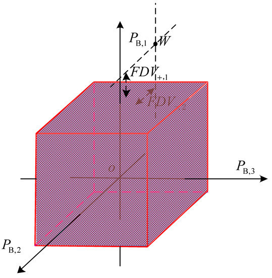
Figure 1.
The FDVs for DN with 3 lines.
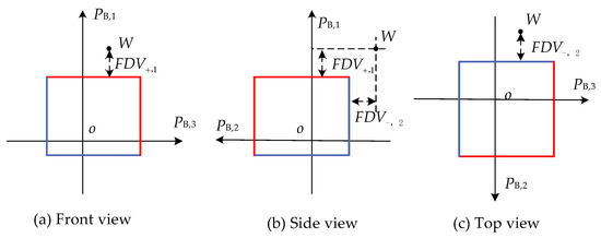
Figure 2.
The three-view drawing of Figure 1.
The forward and reverse FDVs for each line is written in vectors as follows:
where and are the forward and reverse FDVs, respectively; represents the forward FDV for line ; represents the reverse FDV for the line . Calculations of the forward and reverse FDVs are as follows:
where the meaning of in line , as well as and are explained in Equation (1).
2.3. Probability Density Calculation of Line Power with Semi-Invariant
Due to the uncertainties of DGs and loads, the power flows in the DN would be stochastic. For stochastic power flows, as discussed above, security constraints are not guaranteed in some cases. The probabilities and distribution densities of FDVs can be determined through probability power flow calculation.
This paper employs a cumulant algorithm to achieve the indeterminate algorithm. In this algorithm, by calculating the semi-invariant of the initial stochastic quantities, the semi-invariant results is obtained indirectly. According to the nature of semi-invariant, the semi-invariant, the initial stochastic quantities in limited order are substituted to the power flow models to solve the semi-invariant of power flow. Thus, the approximate distribution densities of results are solved with power flow. The following gives the detail of the cumulant algorithm for stochastic power flow.
Let the nodal power injection and voltage be divided into expected and random disturbances. Let the expects are denoted as and for power and voltage, respectively. The random disturbances are represented as and respectively. There are the following relationships between the expects and the random disturbances.
Establish power flow models of the DN and perform Taylor expansion to the quantities. Ignore the higher order terms of the expansion and remain the constant and the 1st order terms only. The power flow expansions with the abandonment of the high orders are as
where is the vector of the nodal power equations; is the vector of the line power flow equations; is the Jacobian matrix of nodal power equations; is a matrix determined by the following relationship as in Equation (8); is the vector of the nodal power injections; is the vector of the line power flows. Note that for approximation, generally, the active power is dependent on the voltage angle on both sides of the line, but the reactive power is dependent on the voltage magnitude. As V is intermediate variable here, the voltage can be expressed no matter which form, such as phasor or power angle. The following equation can be acquired according to Equation (7) and will be eliminated subsequently.
If the probability distributions of the initial random disturbances are known, orders of the semi-invariant quantities are determinable with the origin moments and central moments of the distributions. According to the features of homogeneity and additivity of the independent random semi-invariant quantities, sum the orders of the semi-invariant quantities and are substituted into Equation (7) to obtain each order of the semi-invariant . Since the numerical characteristics of the random variable , as well as the probability density function can be approximately obtained according to their numerical characteristics after the semi-invariant are determined.
According to the above discussions, if the power flows to satisfy the N-0 security constraints, the operating point of DN will be located within the SR of N-0. Else, the OVs will occur. According to the definition of FDV in (3) and (4), the probability densities of FDVs are the same as in the case of the OV state happen. For uncertainty circumstances, general methods such as robust optimization use intervals to treat the uncertainty quantities and deem the cases inner the intervals to have enough confidence to happen. In addition, the security is guaranteed in the worst case among these intervals. Whereas the cases out of the confidence intervals are deemed as risk events, and the security is regardless. After acquiring the power probability distributions of the lines, the power probability of line that meet the N-0 security constraints can be obtained with Equation (9)
The probability of forward and reverse OVs are
where is the probability of forward OVs and is the probability of reverse OVs; is the density function of PB,j.
Through the schedule of the nodal power vector , the line power , as well as the density function, are changed. Changing the probability of security and the bidirectional OVs, the risk conditions are also changed, thus, the operating cost and risk cost are regulated.
2.4. Risk Cost of the OVs
Once OVs occur in some cases, they will inevitably produce losses. Due to the random events that happen occasionally, such losses are risk losses. This paper concerns the OVs caused risk losses in the DNs. If the absorbed powers in some nodes become excessive, some lines may turn to an OV state in forward directions. These situations perhaps happen when the load power is heavy while the renewable DGs power is light. Risk losses caused by load curtailment will be produced. Whereas, if the power injection in some nodes gets excessive, some lines may turn to an OV state in reverse directions. These situations perhaps happen when the load′s power is light while the power of renewable DGs is heavy. Risk losses will be produced with DG generation curtailment and/or flexible load increase. The risk losses of bidirectional OVs are shown in Figure 3.
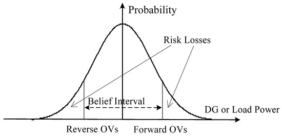
Figure 3.
The risk losses of bidirectional OVs.
The CVaR is used to measure the risk loss caused by the OV events referred to as N-0 SR in this paper. In order to obtain the CVaR, the VaR had to be obtained first. VaR is the maximum loss index at the confidence level. The calculation of VaR for power is in Equation (12).
where is the loss function while the OVs occur in the N-0 state; are the decision variables, designating the scheduled nodal power in the DN for distributed resource; is the VaR under confidence level . CVaR of the PB is calculated with Equation (13)
The general process for calculating is to construct a help function, which is the probability density of power for the total line in a vector.
where ; is an arbitrary real number as in Equation (13).
As there are complex correlations among the probability distributions of the power in each line, it is difficult to calculate with the integral operation. In this paper, Equation (14) is discretized into Equation (15) through typical probability scenarios. Therefore, the probability problem is transformed into a deterministic problem.
where designates the probability of the scenario , designates the total quantity of typical scenarios.
3. Assessment of OV Loss Function for N-0
3.1. Strategies of Anti-Violation for DN
The risk of OVs is the product of the probability and severity of the OV events in reference to SR. When OV events occur in the DN, it is necessary to take action to eliminate the OV events. We call these actions anti-violation strategies (AVS). The more serious the OVs are, the greater the cost of the AVS will expend. In this paper, the severity of OVs is described by the cost of AVS. The available AVS are usually non-unique and with different costs. Therefore, the construction of the optimization model is necessary to obtain the optimal AVS with minimized cost. The loss function mentioned above section is, therefore, determined through optimization.
The AVS is mainly taken by reshaping the power distribution of the DN, including nodal power reshaping and network reshaping. Nodal power reshaping means adjusting the power injections of the DGs, the loads, and the storage of relevant nodes according to the correlation in the OV lines and the nodes, so as to eliminate the OVs. The available nodal power reshaping means comprise:
- (1)
- active regulation of flexible loads;
- (2)
- power curtailment of the rigid loads and the renewable DGs;
- (3)
- altering the charging and discharging of storage;
Power regulations of flexible loads or storage area in bi-ways, namely, are able to be increased or decreased to eliminate the OVs. Such resources are flexible and are the major power reshaping resources. Regulation of rigid loads and renewable DGs are unidirectional, which can be decreased instead of increased. Power reduction in rigid load indicates loss of load and results in an outage of users. Thus, the cost is high. Similarly, power curtailment of renewable DGs implies unexpected abandonment of wind or Photovoltaic (PV) generations and causes penalty costs also. Nodal reshaping resources are multi-time scaled. Storage, DGs, and part of flexible loads can be regulated in real-time. Rigid loads and some flexible loads need to be notified in advance, which is non-real time. Network reshaping is realized through operating mechanical or soft switches to change the power flow distribution of the DN to eliminate the OVs. It is unsuitable for response to the OVs in real-time also. Therefore, this paper only considers the nodal reshaping of AVS. An optimization model is established for the optimal AVS.
3.2. Relationship of FDVs and Nodal Reshaping Power
Let the total lines in the DN are ; the total nodes are ; the power injection vector of nodes is , nodal voltage vector is ; power flow vector of lines is . Based on Equation (7), the power vector of lines can be determined with the power flow equations. Then the line′s power flow is substituted into the boundary of the SR, and the vector of FDV is obtained from Equations (3) and (4), where .
If OVs occur, the DN will actively adjust the nodal power to implement AVS. The power flow equations after implementing AVS are as
where is the nodal power injection after implementation of AVS, is the adjusted amount of nodal power required for AVS; is the nodal voltage after implementing AVS, is the variation amount of nodal voltage after implementing AVS; is the power of lines after implementing AVS, is the power variation amount of lines after AVS. If the power of the OV in a line is just on the boundary after AVS, then
where is the regulating amount of power vector in lines exactly located in SR by the AVS. The following equation can be obtained according to (14)
Equation (18) depicts the relationship between FDVs and the variation of nodal power. Meanwhile, this relationship also explains the required quantity of nodal power modification with the AVS to eliminate the OVs. Based on this relationship, the nodal power modification is able to be determined. Note that Equation (18) has multi-solution. Therefore, the optimization method is imposed on it to solve the optimized solution as discussed in the next section.
3.3. Optimization Model of Nodal Reshaping for AVS
Assume the FDV in the DN for a scenario is . The nodal power regulation is taken to implement AVS. According to the relationship between the regulated power of the AVS as in Equation (17), represented as with , and the distance of OVs represented with , the optimization model of AVS is able to be established with the objective of minimizing the AVS cost.
Assuming the AVS cost of unit power for each node is
where is the unit regulating the cost of the node. Then the total cost of nodal power reshaping in the DN is
Based on the analysis above, the optimization model of nodal power reshaping strategy with the objective of minimizing AVS cost can be established.
- (1)
- The objective
- (2)
- Equality constraints
The Equality constraints are the power flow relationship in Equation (18).
- (3)
- Inequality constraints
The inequality constraints are the permeable forward and reverse range of the nodal power modification.
where and are the allowed range of forward and reverse power in node .
By solving the above optimization model, the optimal modification quantity as of the nodal power to eliminate the OV is available. In addition, the minimum AVS cost can be obtained accordingly. Since the minimum AVS cost is a function of FDV, thus the loss function can be rewritten as .
4. Dispatch Models of DN Considering Risk Cost of OVs
4.1. Modeling of Dispatch for DN
The DN Operator (DNO) implements integrated dispatch to the distributed resources in each node of the DN to minimize the total cost, including the risk cost and operating cost of the DN. The dispatched distributed resources comprise DGs, energy storage, flexible loads, etc. This paper takes the nodal as a decision variable instead of the equipment power in detail. The nodal power consists of rigid loads, flexible loads, energy storage, DGs, and other equipment. The nodal power is the sum power of all equipment in that node. Due to the randomness of renewable DGs and loads, there are deviations between the actual value and the predicted one of nodal power. Assume distributions of the deviation follow the normal distributions. After the dispatched power of the node is determined, the power of each piece of equipment at that node can be easily determined according to the scheduling cost of the equipment. The objective scheduling function with risks can be written as
where is the total cost of the DN; is the risk cost of OVs against the N-0 security boundary; is the scheduling cost of the adjustable equipment, and is the power purchasing cost from the main grid.
For multi-period scheduling problems, the dispatch cycle is divided into K periods. In period , the cost of power purchasing from the main grid is
where is the unit price of power purchasing or selling between DN and the main grid during the period . The scheduling cost includes the cost of flexible loads, storage, and DGs. Let the total scheduling cost in node is , then
where is the flexible loads scheduling cost; is the storage scheduling cost; is the DG scheduling cost.
Assuming DN has nodes, the OV risk cost, the scheduling cost, and the power purchase cost in all nodes and all periods are shown below.
where is the risk cost of OVs against the N-0 security boundary of the DN with nodal power in period .
In addition to the constraints of the power flow equation, the scheduling models also require the constraints of energy storage and flexible loads. Energy storage constraints include charge and discharge inequality constraints. Let charging and discharging power in node and period are , the constraints of are shown below
where and are the nominal charging and discharging power of the storage, respectively.
The calculation and constraint of SOC are
where and are the SOC of storage in node at period and ; is the efficiency of storage, and are the allowable limit of SOC for the storage.
The flexible loads should meet the constraint as
where is the flexible load in node period ; is the max flexible load′s curtailment in node period .
The other equality and inequality constraints are similar to the routine dispatch of DN and will not be repeated in this paper.
4.2. Implementation Process of the Dispatch Containing OV Risk
Based on the optimized scheduling model above, this paper uses the particle swarm optimization (PSO) algorithm to optimize the dispatching scheme. The process is as follows.
- (1)
- Input the basic data, including power flow parameters, nodal power injection as well as their probability densities, various costs of the DN, parameters of particle swarm algorithm, etc. According to power flow calculation, Equation (7) is determined, and therefore the relationship between nodal power alternating and the FDVs can be described.
- (2)
- Build the objective function and constraints, and deduce the dispatch models of the DN.
- (3)
- Initialize the particle swarm algorithm, including the dimensions of the population, the initial position and the speed of particles, the number of iterations, termination conditions, the inertia weight, and the learning factor.
- (4)
- The particle positions are substituted into the DN scheduling model to calculate the nodal power injection. Then substitute the nodal power into the risk calculation of OVs described in 2.4 to determine the corresponding risk. The OV risk is then substituted into the optimization model of DN scheduling to calculate the objective function as the fitness of the particles.
- (5)
- Update the individual optimal value of particles according to particle fitness and the optimal global valuewhere is the element of the particle ; is the element of lase iteration particle ; is the element of velocity for particle , is the element of lase iteration velocity for particle ; is inertia weight; and are constant values; and are random values.
- (6)
- Repeat steps (4) and (5) until the termination conditions are met. The global optimized scheme of dispatch is then obtained.
According to the above steps, the scheduling optimization can be realized considering OV risk.
5. Example Analysis
5.1. IEEE-33-Bus Distribution System
In this paper, the IEEE-33 DN system (Figure 4) was used for the dispatch model study.
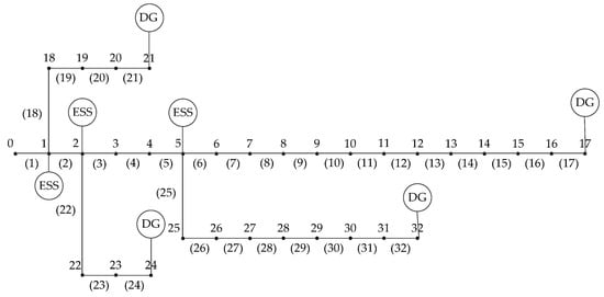
Figure 4.
Example of the IEEE-33 node system.
The system has a reference voltage of 12.66 kV, a reference power of 10 MW, 33 nodes, and 32 lines. No. 0 is a slack node. The compensation of FL, PV, and ES is given by the DNO and established with reference to the compensation price in the market. Each node contains 25% of FLs for dispatching. The economic compensation standard of FLs is shown in Table 1. Five categories of users are classified in Table 2. Different user has a different cost of AVS. Nodes 17, 21, 24, and 32 are connected with PVs, and Nodes 1, 2, and 5 are connected with electricity storage (ES). ES and PV parameters are shown in Table 3. The PV of each node provides the same amount of power in each period. The PV power generated curve, power consumption curve, and power purchasing price curve of DN are shown in Figure 5. For the optimization parameters, the number of particle elements is 30, and the maximum number of iterations is 1000. The value of and is , and is set based on Equation (32).
where is the maximum number of iterations; is the actual number of iterations. For the population, the decision variables for the optimization are the power of dispatched with FLs, ES, and PVs. The scheduling periods are 24 h ahead, which are equally divided into 24 periods.

Table 1.
Components inside the distribution station area.
Table 2.
Types of loads and losses in the node.
Table 3.
Parameters of distributed energy sources.
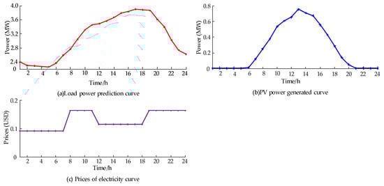
Figure 5.
Power prediction for PV and loads and power purchasing price curves.
5.2. Dispatch Optimization Results
5.2.1. OV Risk before Scheduling
By using the method described in Section 4, a model was constructed to calculate the violation risk in the N-0 security region of the DN with day-ahead scheduling. The power injected into each node follows a normal distribution that is independent of the distribution of other nodes. The probability density function of the power injected into each node is constructed with the maximum range of fluctuation in expectation being . The predicted load values are shown in Figure 6. The red lines show the expected load values, and the fluctuation range is shaded.
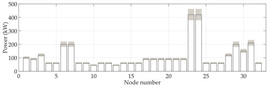
Figure 6.
Prediction of nodes′ power curves.
To better describe the violation in the security region with the operation scenario of the DN, the expected power is regarded as the power injected at the node. The direction of power flow in this scenario is considered as the forward direction, and the flow is regarded as the forward power constraint of the branch. It is assumed that there is no reverse power in the network. The N-0 security region is constructed with parameters for power constraints, as listed in Table 4.
Table 4.
Parameters for power constraints of DN branches.
In this scenario, probabilistic power flow calculation is carried out to obtain the maximum confidence that the power of distribution network lines does not exceed the limit. The results of some lines are shown in Figure 7.
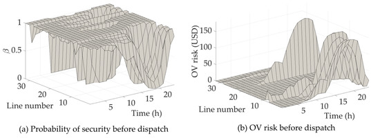
Figure 7.
Security Probability and OV risks before dispatch.
Figure 7a shows a certain probability of an OV event. Therefore, the DN network cannot fully meet the N-0 security and have certain OV risks. In this scenario, the OV risk of the DN can be obtained. The OV risks are shown in Figure 7b. According to Figure 7b, the OV risks particularly show a high level in lines 1–10 and lines 22–24, although almost every line has a high OV probability in some events. This phenomenon is due to the AVS costs of different lines. Due to the high AVS cost of connected nodes and the high probability of OV events, the OV risk in lines 1–10 and lines 22–24 increases significantly. The above analysis is based on the sunny days PV characteristics. If the weather changes to cloudy, the PV power generated would drop significantly, and the power drop in the period will become uncertain. Refer to the PV power generated curve in Figure 5b, plot the PV power curve of cloudy days as shown in Figure 8a, and the probability of security of cloudy days is shown in Figure 8b.
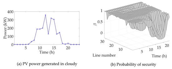
Figure 8.
PV power generated and security probability during cloudy weather.
It can be seen from the results that the security probability of the line that is not connected to PV has decreased a little compared with normal days, but due to the reduction in PV power, the security probability of the line connected to the PV shows a significant improvement.
The above analysis shows that the proposed risk model for the security region of the DN can obtain the level of violation and determine the OV risks for each time period based on the network architecture, characteristics of power injected into nodes, and cost of countermeasures against violation in the lines. Therefore, the OV risk model proposed in this paper for the N-0 security region of the DN can be used to obtain the corresponding OV risk based on the nodal power in a given security region and costs for countermeasures against violation.
5.2.2. Optimized Scheduling Results
Based on the day-ahead scheduling process described in Section 4, a model was established for day-ahead dispatch optimization of the DN, and the results were obtained. Optimization was performed to minimize the total costs of the DN while considering the electricity purchase cost, cost of scheduling distributed resources, and risk cost of the violation. The results are presented in Figure 9.
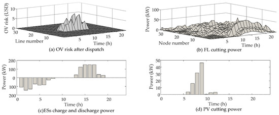
Figure 9.
Optimized OV risks and dispatch results.
Figure 9a shows the risk of forwarding OV referred to the security region of the DN with the minimum total operating cost. A comparison of the OV risk of the DN before and after optimization shows that before optimization, the peak OV risk value was 167.6 USD in 18 h, and in node 22, the total duration of OV was 13 h. After optimization, the total duration of the forward violation was reduced to 14 h, with a peak value of 7.93 USD in node 13. These results show that the optimization model can significantly reduce the violation risk of the DN. Figure 8b shows the FLs dispatch result. From Figure 7b and Figure 9b, although only in lines 1–10 and lines 22–24 exists a high level of OV risk, FLs curtailment is present on almost all nodes to reduce OV risk due to the compensation characteristics of FLs. Figure 9c,d show the power dispatching results of ESs and PVs in the DN. Since the dispatch results of each ESS and PV have a smaller difference, Figure 9c,d only gives the total dispatch results. It can be seen from the figure that the ESs are charged during the low electricity price period and chooses to discharge during the normal electricity price period when the OV risks are high. The PV also has power curtailment when reverse OV appears. These results are followed by the expectations that the optimization can dispatch DGs to avoid risks and reduce costs.
To analyze the effect of the optimization strategy on the total costs of DN, the risk optimization (RO) proposed in this study was compared with the deterministic optimization (DO) and traditional robust optimization (TRO) methods [8]. DO and ROMIC are solved by the PSO method and have been simplified and changed based on the reference method to make it fit the example this paper mentioned. In order to analyze the economic benefits of the three methods, the electricity purchase cost, scheduling cost, and violation risk cost as indicators were introduced. The results of the comparison are shown in Table 5.
Table 5.
Distribution network operating cost parameters for different scheduling schemes.
The result shows that the RO method has the lowest total DN costs. DO method does not consider the prediction error of DN during optimization, which leads to a higher OV risk cost. Although the DO method has the lowest dispatch cost and power purchase cost than the other two methods, the total cost is the highest among the three methods. TRO method considers the worst case of all scenarios; thus, TRO has the lowest risk of OV and the highest dispatch cost among the three methods. In addition, due to a large amount of load curtailment, the power purchase cost of the TRO method is also lower than that of the RO method. Compared to the other two methods, the RO method still has a lower risk cost, although the OV risks cost, dispatch cost, and power purchase cost are not the lowest of the three methods. The result shows that the RO of balancing the economy with dispatch cost and power purchase cost and the security with OV risks can achieve better efficiency. The scheme described in this paper precisely plans the dispatching scheme of distributed resources so that it can obtain the highest removal efficiency of over-limit risk and realize the unified dispatching of distribution network economy and security.
6. Conclusions
In order to solve the uncertainty scheduling problem in complex scenarios of DN, this paper has proposed an economic scheduling method that considers both the risk cost of OV at N-0 and the conventional operating cost. The bidirectional distance of OV is constructed and referred to as SR, with which the overloading problem could be investigated in the SR framework. Performing the optimal AVS in the optimization formula and as the loss function, thus gaining the most economical anti-violation scheme, this way is in agreement with the overall objective and can lessen the total cost of the schedule further. In addition, the cumulant algorithm successfully accomplished the calculation of the probability density of line power according to nodal power. Similarly, the CVaR index is feasible in quantifying the cost of risk. The method incorporates the economic risk caused by AVS into the economic evaluation of the DN and constructs an optimal objective function considering the risk cost of OV. This paper also provides a strategy to solve the DN uncertainty. Instead of the traditional dispatch strategy with fixed security limits, the essence of this strategy is to adjust the security risk to the proper level from an economic aspect. Using the optimization algorithm to balance risk cost to obtain a more efficient dispatch strategy. The results show that the optimal scheduling model proposed in this paper formulates a more cost-effective distribution network scheduling strategy by reducing the serious OV risks to control the risk level and decrease the total cost, including risk cost and operating cost. According to the example, the method proposed in this paper can obtain a more efficient DN dispatching scheme compared with RO or TRO method.
This model considers the real power OV risk of the distribution network. Future research will focus on other security-affected factors that have less consideration in this paper, such as the definition of the feeder distance and anti-violation strategies of voltage and reactive power. Meanwhile, the influence of reactive power on the method and the tackle are owed to investigate deeply. In addition, for more complicated fluctuation characteristics and economic accounting indicators, DN system. Future research will work on how to provide a more precise description of the above parts based on existing models.
Author Contributions
Conceptualization, G.Y. and J.J.; methodology, J.J.; software, J.J.; validation, J.J., G.Y. and L.S.; formal analysis, J.J.; investigation, J.J.; resources, L.S.; data curation, L.S.; writing—original draft preparation, J.J.; writing—review and editing, J.J.; visualization, J.J.; supervision, A.A.-S.; project administration, G.Y.; funding acquisition, L.S. All authors have read and agreed to the published version of the manuscript.
Funding
This research was funded by National Natural Science Foundation of China grant number 51877186. And The APC was funded by Yanshan University.
Conflicts of Interest
The authors declare no conflict of interest.
References
- Zhou, K.; Mohy-ud-din, G.; Agalgaonkar, A.P.; Muttaqi, K.M.; Perera, S. Distribution System Restoration with Renewable Resources for Reliability Improvement Under System Uncertainties. IEEE Trans. Ind. Electron. 2020, 67, 8438–8449. [Google Scholar] [CrossRef]
- Li, Y.; Wang, Y.; Chen, Q. Optimal Dispatch With Transformer Dynamic Thermal Rating in DNs Incorporating High PV Penetration. IEEE Trans. Smart Grid 2021, 12, 1989–1999. [Google Scholar] [CrossRef]
- Xiao, J.; Guo, W.; Zu, G.; Gong, X.; Li, F.; Bai, L. An observation method based on N-1 simulation for distribution system security region. In Proceedings of the 2016 IEEE Power and Energy Society General Meeting (PESGM), Boston, MA, USA, 17–21 July 2016; pp. 1–5. [Google Scholar]
- Xiao, J.; Qu, Y.; Zhang, B.; She, B.; Lin, Q. Security Region and Supply Capability of Urban Distribution Network with N-0 Security. Autom. Electr. Power Syst. 2019, 43, 12–19. [Google Scholar]
- Zhang, Z.; Wang, C.; Lv, H.; Liu, F.; Sheng, H.; Yang, M. Day-Ahead Optimal Dispatch for Integrated Energy System Considering Power-to-Gas and Dynamic Pipeline Networks. IEEE Trans. Ind. Appl. 2021, 57, 3317–3328. [Google Scholar] [CrossRef]
- Zhang, Z.; Shi, J.; Yang, W. Deep Reinforcement Learning Based Bi-layer Optimal Scheduling for Microgrid Considering Flexible Load Control. CSEE J. Power Energy Syst. 2022, 1–14. [Google Scholar] [CrossRef]
- Zhang, C.; Xu, Y.; Dong, Z.Y.; Ma, J. Robust Operation of Microgrids via Two-Stage Coordinated Energy Storage and Direct Load Control. IEEE Trans. Power Syst. 2017, 32, 2858–2868. [Google Scholar] [CrossRef]
- Luo, L.; Nie, Q.; Yang, D.; Zhou, B. Robust Optimal Operation of Active Distribution Network Based on Minimum Confidence Interval of Distributed Energy Beta Distribution. J. Mod. Power Syst. Clean Energy 2020, 9, 423–430. [Google Scholar] [CrossRef]
- Wang, B.; Dehghanian, P.; Zhao, D. Chance-Constrained Energy Management System for Power Grids With High Proliferation of Renewables and Electric Vehicles. IEEE Trans. Smart Grid 2020, 11, 2324–2336. [Google Scholar] [CrossRef]
- Tang, K.; Dong, S.; Ma, X. Chance-Constrained Optimal Power Flow of Integrated Transmission and Distribution Networks With Limited Information Interaction. IEEE Trans. Smart Grid 2021, 12, 821–833. [Google Scholar] [CrossRef]
- Yuan, Z.; Xia, J.; Li, P. Two-Time-Scale Energy Management for Microgrids With Data-Based Day-Ahead Distributionally Robust Chance-Constrained Scheduling. IEEE Trans. Smart Grid 2021, 12, 4778–4787. [Google Scholar] [CrossRef]
- Tang, H.; Wu, J.; Chen, L.; Liu, Z.; Wu, F.; Li, K.; Wu, Z.; Yu, F.; Bi, Q. A Control Optimization Model for CVaR Risk of Distribution Systems with PVs/DSs/EVs Using Q-learning Powered Adaptive Differential Evolution Algorithm. Int. J. Electr. Power Energy Syst. 2021, 132, 107209. [Google Scholar] [CrossRef]
- Khodabakhsh, R.; Sirouspour, S. Optimal Control of Energy Storage in a Microgrid by Minimizing Conditional Value-at-Risk. IEEE Trans. Sustain. Energy 2019, 7, 1264–1273. [Google Scholar] [CrossRef]
- Rosewater, D.; Baldick, R.; Santoso, S. Risk-Averse Model Predictive Control Design for Battery Energy Storage Systems. in IEEE Trans. Smart Grid 2020, 11, 2014–2022. [Google Scholar] [CrossRef]
- Vahedipour-Dahraie, M.; Rashidizadeh-Kermani, H.; Shafie-Khah, M.; Catalão, J.P. Risk-Averse Optimal Energy and Reserve Scheduling for Virtual Power Plants Incorporating Demand Response Program. IEEE Trans. Smart Grid 2021, 12, 1405–1415. [Google Scholar] [CrossRef]
- Ju, L.; Zhao, R.; Tan, Q.; Liu, Y.; Tan, Q.; Wang, W. A multi-objective robust scheduling model and solution algorithm for a novel virtual power plant connected with power-to-gas and gas storage tank considering uncertainty and demand response. Appl. Energy 2019, 250, 1336–1355. [Google Scholar] [CrossRef]
- Yang, S.; Tan, Z.; Guo, S.; Li, P.; Ju, L.; Zhou, F.; Tong, X. Optimization Model of WPO-PVO-ESO Cooperative Participation in Day-ahead Electricity Market Transactions Considering Uncertainty and CVaR Theory. Int. J. Electr. Power Energy Syst. 2021, 129, 106718. [Google Scholar] [CrossRef]
- Zhang, Y.; Zhao, H.; Li, B.; Zhao, Y. Research on Credit Rating and Risk Measurement of Electricity Retailers Based on Bayesian Best Worst Method-Cloud Model and Improved Credit Metrics Model in China′s Power Market. Energy 2022, 252, 124088. [Google Scholar] [CrossRef]
- Eslahi, M.; Vahidi, B.; Siano, P. A Flexible Risk-Averse Strategy Considering Uncertainties of Demand and Multiple Wind Farms in Electrical Grids. IEEE Trans. Ind. Inform. 2022, 18, 2255–2263. [Google Scholar] [CrossRef]
- Xiao, J.; Wu, G.; Wang, C. Distribution System Security Region: Definition, Model and Security Assessment. IET Gener. Transm. Distrib. 2012, 6, 1029–1035. [Google Scholar] [CrossRef]
- Xiao, J.; Zu, G.; Gong, X. Observation of Security Region Boundary for Smart Distribution Grid. IEEE Trans. Smart Grid 2017, 8, 1731–1738. [Google Scholar] [CrossRef]
- Xiao, J.; Zhang, B.; Luo, F. Distribution Network Security Situation Awareness Method Based on Security Distance. IEEE Access 2019, 7, 37855–37864. [Google Scholar] [CrossRef]
- Xiao, J.; Zhen, G.; Wang, B.; Wang, C. Security Distance of Distribution Network: Definition and Method. Proc. CSEE 2017, 37, 2840–2851. [Google Scholar]
Publisher’s Note: MDPI stays neutral with regard to jurisdictional claims in published maps and institutional affiliations. |
© 2022 by the authors. Licensee MDPI, Basel, Switzerland. This article is an open access article distributed under the terms and conditions of the Creative Commons Attribution (CC BY) license (https://creativecommons.org/licenses/by/4.0/).