Abstract
Pick-and-place operations are basic, and are currently the most common for robots operating in the industry. Massive applications makes it reasonable to ask whether, and to what extent these operations are realised in a way that guarantees rational energy consumption. In many cases, the answer to such a question is neither positive nor known. Therefore, this paper attempts to present a rational and systematic approach to the low-energy pick-and-place operations performed by robots. This paper describes a new approach for the robot’s tool centre point path planning, which enables the minimisation of energy consumption wherein productivity in preserved, and where care is taken for the persistence of the critical mechanical components of the robot cooperating with the autonomous mobile platform. The effectiveness of the described approach has been proven from the results of the theoretical, simulation, experimental and implementation tests carried out using an industrial articulated robot with six degrees of freedom.
1. Introduction
Pick-and-place operations are the most frequently performed processes among the tasks performed by six-degrees-of-freedom (6DoF) robots in the industry. It has been estimated that this type of operation comprises over 50% of all processes carried out by modern industrial robots [1]. Generally, such operations consist of transferring an object between a pick and a deposit point, with consideration being given to existing space limitations. The pick-and-place operations include such technological processes as palletising, assembly, packing and selection. Operations such as these usually require the synchronisation of movements of the object with the respective operations of the technological process. As a result, pick-and-place operations are subject to particular time restrictions. The most crucial is the transfer cycle duration. The transfer cycle duration is determined by the time interval required for a complete performance of the transfer operation. The reverse of this interval defines the process productivity. In the later parts of this paper, we will also refer to specific energy consumption, i.e., the energy needed for the performance of a single pick-and-place cycle.
Some pick-and-place operations are presently carried out by 6DoF robots mounted on autonomous mobile robots (AMR). AMR robots are involved mainly in operations such as transfer, logistics and inspection. These operations are performed in an unmanned and environmentally safe manner [2,3]. The integration of a mobile AMR-type robot and an articulated 6DoF robot is advantageous, especially in highly automatised processes characterised by relatively frequent changes in transportation tasks.
This paper will focus on the extremely important and current issue of minimisation of specific energy consumption using an assembly of an articulated 6DoF robot and a mobile AMR platform. It will be shown that such a solution makes it possible to not only save significant amounts of energy but to also reduce the cost of a single transportation cycle. It must be expressed clearly that in industrial practice, energy consumption reductions are often neglected and sidelined, which as a result brings unwanted costs and energy losses.
In this paper we will propose a novel approach to planning the path and the trajectory of a robot’s tool centre point (TCP), which will facilitate obtaining an optimal solution in the context of one of the three formulated criteria. We will try to answer the question of whether a reduction in specific energy consumption is possible without any simultaneous significant cut in the productivity of the pick-and-place process.
The primary criteria in assessing the correctness of the TCP path planning process for pick-and-place operations is whether and to what extent the path meets the required technological requirements. These requirements usually concern the specification of the pick-and-place operation and the realisation of the requirements of the transportation cycle. Therefore, in the general case, it is to be expected that the decided requirements may either be achievable or not, and not necessarily in only one way. If there is more than one solution, additional path planning constraints can be imposed. This will narrow down the set of possible solutions and support the realisation of the technological requirements, and also have an impact on the rationalisation of the technological process.
It is well worth noting that this problem has not been presented as comprehensively in the path planning literature so far. Ratiu and Prichici [4] proposed the following three criteria for assessing TCP path quality:
- Minimum cycle time duration;
- Minimum energy consumption, minimum total torque or minimum driving force;
- Smoothness of the higher-order derivatives of trajectories.
It often happens that the evaluation of path quality is partial and consists of an assessment relating to just one criterion. For different classes of operations, the primary criteria may just be the minimum cycle time, and in other cases, a minimum energy consumption, and in still others, the precise tracking of the planned trajectory. In all of the cases, however, the key element of the path planning process is to provide such a path that is achievable in order to obtain a smooth trajectory, i.e., a trajectory that is characterised by the continuity of the higher-order derivatives of the path, such as velocity, acceleration, and possibly also jerk and snap. It is also important to take care to ensure the durability of the actuators [5]. In practice, in many cases it is necessary to reach a compromise solution that takes into account several criteria [6,7]. Due to the multi-criteria assessment of the correctness of path planning, the task of aiming to generate paths appropriately is certainly not a trivial one.
The problem of low-energy consumption has recently been heavily explored in works on robotics. Carabin [8] presents a general classification of energy optimisation methods, which includes two main classes:
- Optimisation based on hardware solutions;
- Optimisation based on software solutions.
Various approaches to energy minimisation based on hardware solutions are presented in papers [9,10,11,12,13,14,15,16], among others, focusing on ideas and research on developing dedicated structural and material solutions. Numerous designs for robot kinematics, structures, materials and components have been recommended to minimise the energy consumption for a determined pick-and-place operation. The aforementioned papers refer to robots that are limited to two or three degrees of freedom. Such robots, however, are not commonly used due to the limited workspace and manipulation capabilities of the TCP. Some of the papers show hardware optimisation approaches such as parallel robots with enclosed kinematic chain structures [17,18]. They allow for the minimisation of energy consumption; however, they also require the use of additional components (e.g., joints or connectors), which increases the complexity and cost of robot manufacturing and operation.
Most of the papers that are related to the software optimisation of energy consumption have focused on developing the path planning and generating trajectories that allow for the minimisation of certain aggregates that are related to the driving torques and/or forces developed by the robot’s actuating systems [19,20,21,22,23]. Such approaches allow not only for the reduction of energy consumption, but also for an increase in the durability of the drive components, and thus indirectly improve the functional safety of the robot. This is extremely important in the next-generation robots [24,25,26,27], especially those in which harmonic gears are used in the joints. This is due to the fact that, despite numerous advantages, harmonic gears are characterised by a strong decrease in durability in relation to the torque load [28]. A significant shortcoming in the papers mentioned above is that they do not consider the problem of minimising energy consumption directly. The minimisation of torque or cycle time can be only a part of the task of minimising energy consumption, and cannot be equated with a holistic solution.
There is a group of papers that present an attempt to minimise energy consumption for both: an arbitrarily defined trajectory and a point-to-point transport task, with starting and endpoint fixed but without an a priori defined TCP path. Paes [29] presents an approach where the dynamic parameters are estimated and the robot model is developed in MATLAB, using its tools to estimate robot dynamics model and to optimise trajectory. Boscariol [30] proposes functional redundancy as a way to minimise energy consumption. Depending on the task, some of the robot’s effectors could be inoperative, resulting in a reduction in the number of degrees of freedom. In a number of recent papers on minimising energy consumption in robotics [31,32,33] an iterative dynamic programming algorithm was applied and an energy characteristic parameter model based on dynamic time-scaling was developed. A limitation of the above-mentioned papers is that the optimisation only works in terms of the already assumed initial and final configurations of the robot. The authors do not analyse or examine the impact of the choice of the robot’s base location on the specific energy consumption. If the robot is not properly positioned in the task space, only an intermediate goal can be achieved by minimising the energy in this configuration.
The works [34,35,36] have attempted to optimise the trajectory by considering the position of the robot base in the task space. The optimisation only concerned the cycle execution time. In addition, the authors presented examples of virtual trajectories not actually possible for application in industrial practice.
An approach to minimising energy consumption using a swarm algorithm for a 6DoF robot is presented in the paper [37]. However, the authors failed to develop an effective analytical model suitable for simulation studies, making the optimisation process cumbersome and time-consuming, as it required hundreds of experimental tests on a real-world bench. Zhang [38] used a neural network to develop a model and to predict the energy consumption with a set of kinematic parameters as input and energy consumption as the output. The authors considered the energy cost as the optimisation criterion, but they ignored the efficiency of the process. This means that the solution cannot be regarded as being comprehensive in terms of planning the robot’s trajectory in practical industrial terms.
In this paper, we propose a new approach to optimising the trajectory of a 6DoF articulated robot for pick-and-place tasks based on software optimisation solutions and the selection of optimal robot placement. We demonstrate that the location of the robot’s base has a significant impact on the energy consumption and as such, it should be taken into account when taking a holistic view of the problem of energy conservation.
This approach allows for:
- Minimising the specific energy consumption of the transport cycle;
- Minimisation of transport cycle time;
- Minimising the economic cost of realising the transport cycle.
The above criteria are strongly justified from a practical perspective, as they directly determine the economics of the process, including the potential for energy savings. In this paper, tests will be carried out wherein real conditions will be preserved, as well as the resulting limitations on the values of the maximum speeds and accelerations.
First of all, in the scope of the literature study carried out, this paper fills a gap in the research focusing on the economics of robotic production processes. Apart from that, the paper’s important contribution to the field of robotics is:
- A proposal of a new, energy-efficient and implementable approach to path and trajectory design by optimising the trajectory of TCP and solving the 6DoF robot placement problem.
- The industrially acceptable solution for setting an optimal position of the robot integrated with an autonomous mobile platform.
- The proposal of cost-cutting for pick-and-place operation via a multi-criteria optimisation, where both energy consumption and process efficiency are addressed.
- Experimental proof of the proposed approach.
The paper is structured as follows. Section 1 formulates the problem of energy minimisation in automated pick-and-place transport tasks. A review and analysis of the selected literature in this area is presented, and the basic contribution and novelty elements of the article are formulated. Section 2 presents an in-depth characterisation of the pick-and-place tasks. Section 3 outlines the proposed approach, and the methodology selected and tools used. In this section, a description of the analytical model used for the study is presented. Section 4 defines the optimisation task for different criteria. Section 5 presents the technical characteristics of the industrial articulated 6DoF robot used for the experimental study. Section 6 presents the results of a simulation and experimental study of the influence of the robot’s location in the pick-and-place task space on energy consumption, transport cycle execution time and specific cycle cost. Section 7 discusses and draws conclusions from the results obtained, and finally, Section 8 presents a summary of the work.
2. Characterisation of the Pick-and-Place Tasks
A statistical analysis of the number and type of industrial applications developed by the International Federation of Robotics (IFR) [1], indicates that more than 50% of all tasks performed by industrial robots fall into the pick-and-place category. Pick-and-place tasks involve moving an object of manipulation from a pick point to a put-down point. According to the IFR classification, technological processes such as assembly and transport processes, including palletisation and packaging, belong to this task class (Figure 1).
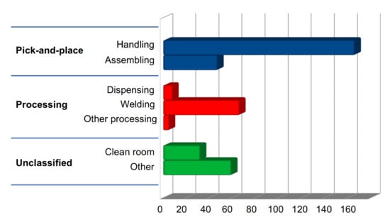
Figure 1.
The annual number of newly installed robots in 2020, in thousands of pieces, broken down by categories of tasks. There are three main task categories: pick-and-place, processing and unclassified. The drawing was elaborated based on [1].
Path planning is usually carried out by searching for a so-called set of waypoints. A set of waypoints is an ordered list of geometric coordinates of reachable points in the programming space that satisfies the kinematic constraints of the robot and the constraints imposed by the task space.
The set of waypoints between the pick-up point and the drop-off point determines the so-called admissible solution of the robot path in the task space. The admissible solution is the starting point for trajectory selection and transition function construction. The trajectory is one of the possible admissible paths, while the transition function defines the time sequence of the robot effector controls leading to the realisation of the selected reachable trajectory, i.e., one for which there is a finite sequence of controls and intermediate states carrying the system from the initial state to the final state. An optimal selection of the trajectory and the associated transition function requires the solution of an optimisation task. Much work in path planning has been devoted to mono-criteria optimisation based on:
- The minimisation of task execution time [39,40];
- Minimising the length of the trajectory [41,42];
- Minimising the energy required for the task execution [30,37].
The discussion in Section 1 shows that considering only one optimisation criterion significantly limits the search space, as it does not take other criteria. For example, the postulate to minimise the execution time of a transport task usually does not allow for a simultaneous minimisation of the energy required for this task.
From a practical point of view, mono-criteria optimisation does not consider many important constraints (limitations) imposed on the transport task. The way out is to adopt a compromise solution consisting, for example, of selecting a technologically acceptable transport cycle while minimising the energy consumption, i.e., generating the transition function in such a way where the so-called effector effort [5] is not excessive. This implies the desirability of using approaches from the area of multi-criteria optimisation with an appropriately designed cost function.
An important practical aspect that is not taken into account in many trajectory planning approaches is the fact that both the pick-up and put-down locations are often only determined after, and not before, the robot is physically installed in the production line. From the point of view of the optimisation task, the location (anchoring) of the robot base relative to the pick-up and put-down positions, is not indifferent. Relevant research in this direction has been carried out in this paper.
3. Minimisation of Specific Energy Consumption
We propose a general and systematic approach to minimising specific energy consumption in pick-and-place operations. The approach consists of three successive steps:
- The determination of an analytical model of the electric energy consumption of each robot drive as a function of the geometric, kinematic, and dynamic parameters;
- The design of a function to determine the cost and constraints of a trajectory optimisation task;
- Performing optimisation calculations.
Step one is closely related to the kinematics of the robot. This means that an individual approach is required for each robot design type. This step consists of a sequence of transformations that lead from the definition of the pick-up and put-down points to the estimation of the electrical energy required for the task. The sequence of transformations is presented in a compact graphical form in Figure 2 and is described in more detail in Section 3.1.
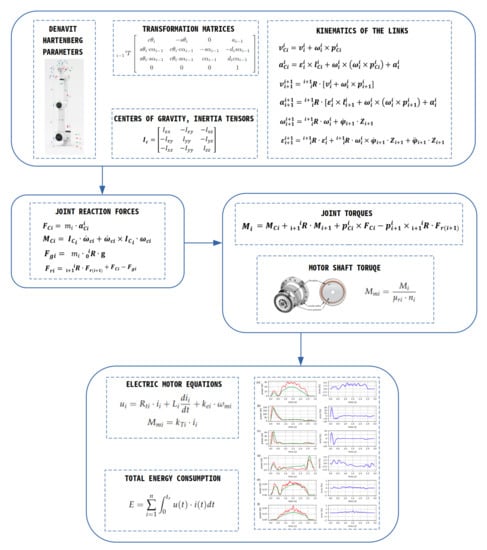
Figure 2.
Graphical diagram of the process of deriving the analytical model of energy consumption.
In step two, the objective of the optimisation task is defined. This step is partly universal in the sense that, at the level of functional definition, it is not related to the construction type of the robot. However, at the level of defining constraints, it does. At this stage, the problems of minimising energy consumption, minimising the transport execution time and minimising its economic cost are defined. The solution of the optimisation problem allows for the definition of the trajectory, the transition function and the location of the robot with respect to the task space, according to the optimisation objective function.
The third step is technical and is related to the implementation of the optimisation task. The choice of method and the technical means of optimisation can be arbitrary. This paper proposes the use of Kennedy and Eberhart’s particle swarm algorithm (PSO) for this purpose [43].
3.1. The Analytical Model
The transport task is a dynamic process. This paper will present both an analytical model of the total energy required to complete the task, as well as detailed (partial) models of the energy consumption relating to the individual drives of the robot joints. The development of such a models requires knowledge of both the robot’s kinematics, and its mechanical and electrical parameters. This paper will present a general method for determining the model for the case of an articulated 6DoF robot. The proposed approach requires the solution of the following three tasks:
- Forward and inverse kinematics;
- Forward and inverse dynamics;
- Determining the energy consumption.
By solving the forward and inverse kinematics, it is possible to determine the internal coordinates of the robot, i.e., the angular positions of the joints versus position of the robot’s TCP.
Based on the knowledge of the kinematics and mechanical parameters of the robot, it is possible to present a solution of both the forward and inverse dynamics. By solving this task, it is possible to determine the dynamic forces and torques reacting in the joints of the robot. Thus, after applying appropriate transformations, it is possible to determine the instantaneous power required to drive the individual robot joint and, consequently, the instantaneous and total energy consumption.
3.1.1. Forward and Inverse Kinematics
The forward and inverse kinematics task was solved using the well-known approach represented in [44,45], among others. The method of solving the forward and inverse kinematics will be illustrated using an ES5 robot [27]—the representant of a typical six-articulated robot, whose structural schematic is shown in Figure 3. The approach presented in this paper is universal, although for different robots structures it requires defining individual Denavit–Hartenberg (D-H) parameters and and maybe performing a different sequence of algebraic transformations.
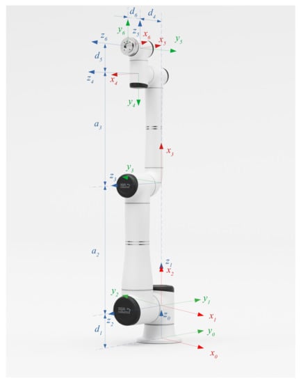
Figure 3.
Three-dimensional drawing of the ES5 robot with assigned local coordinate systems according to the Denavit–Hartenberg representation.
A local coordinate system according to D-H notation [44,46] was assigned to each of the six rotational joints of the robot. The D-H parameters are the geometrical parameters assigned to each joint. In D-H notation, we specify the following four parameters:
- —distance between the and axes measured along the axis;
- —the angle between the and axes;
- —distance between the and axes measured along the axis;
- —angle between the axes and .
The base coordinate system was assumed to be anchored at the geometric centre of the robot base. According to the D-H representation, the single transformation matrix of the coordinate system to can be represented as an Equation (1), being the product of the elementary transformation matrices, where , and are the geometric parameters, is the coordinate associated with the i-th coordinate system, and and are the transformation axes:
where R is a rotation matrix and P is a translation vector. Therefore,
where the symbol s denotes the function sinus and the symbol c denotes the function cosinus.
The forward kinematics consist of determining the coordinates of the position and orientation of the robot’s TCP ( transformation matrix) from known values of internal variables. This task requires the multiplication of all transformations of the entire robot kinematics chain:
For the purpose of inverse kinematics task, we will replace elements of transformation matrix (3) with the rotation and translation symbols ( and ), as in (4).
The inverse kinematics involves determining the internal coordinates of the robot based on knowledge of the transformation matrix, which describes the position and orientation of the coordinate system associated with the robot’s TCP, relative to the base coordinate system.
Determining the coordinates requires a number of complex geometric transformations.
3.1.2. Forward and Inverse Dynamics
We will now consider the tasks of forward and inverse dynamics. In practice, it allows for determining the instantaneous power that is required for robot’s actuating elements. In the case of the forward dynamics, the dynamic parameters of the robot’s TCP are reconstructed, assuming a knowledge of the force vectors and driving torques at the joints. From the perspective of achieving the objectives of the paper, it is much more important to find the inverse solution, i.e., to reconstruct the force vectors and torques acting in the joints of the robot, based on the known trajectory of the TCP. Two approaches are commonly used to solve the inverse dynamics:
- The Newton–Euler method;
- The Lagrange equation of the second kind.
In this paper, we propose the Newton–Euler method due to the simpler form of the equations in explicit form obtained for a multi-member kinematic chain. The Newton–Euler method allows for the recursive determination of the force and torques vectors in all joints of the robot. For this reason, it should be considered as being convenient for the implementation. Figure 4 depicts a flowchart that is helpful for deriving the force and torque equations for the joints of a robot with an articulated structure.
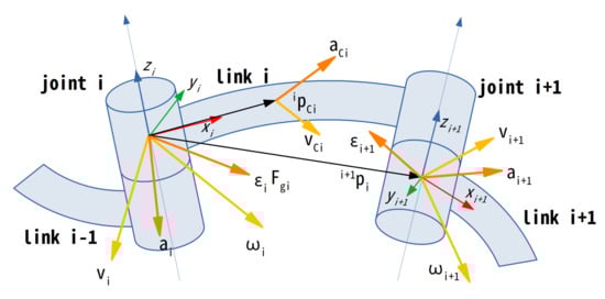
Figure 4.
Kinematics link of the articulated robot.
To do this, we will determine the linear velocity and the linear acceleration of the centre of gravity of each i-th link in the local i-th coordinate system based on the velocity and acceleration of the systems associated with the origins of each link (Figure 4). The procedure is performed for each link starting from the first one.
The linear velocity v, angular velocity , linear acceleration a and angular acceleration in the above equations are described by the formulas (8)–(11):
where:
, velocity and acceleration of the link in the coordinate system associated with the origin of this link,
, rotation matrix and translation vector from the coordinate system i to .
where:
, —speed and acceleration of the joint , determined by solving the inverse kinematics,
—versor of the z-axis of the -th coordinate system.
The knowledge of the inertia tensor of all links of the robot is required for the development of the model of dynamics:
where:
—the coefficients of the main diagonal are the principal moments, the others are the moments of deviation,
—axes of the coordinate system about which the inertia tensor is determined.
The directions and magnitudes of the force and torques vectors are shown schematically in Figure 5.
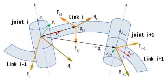
Figure 5.
Forces and torques acting on the robot link.
The values of the forces and moments of inertia of the i-th link’s centre of mass are determined from the Equations (13) and (14):
where:
—the inertia force vector associated with the centre of mass of the i-th link relative to the coordinate system associated with the begining of i-th link,
—the moment of inertia associated with the centre of mass of the i-th link in the i-th coordinate system,
—the mass of the i-th link,
—the tensor of the inertia of the i-th link.
The force of gravity acting on a link i in the coordinate system associated with its origin, can be represented by:
The reaction forces in the i-th joint coordinate system balances its gravitational force, the acting inertia (d’Alembert force), and the reaction force in the joint. The rotation matrix allows for the transformation of the reaction force of the system associated with the joint to the coordinate system associated with the joint i. Hence:
Based on Equations (6)–(16), the sum of the moments of the forces acting on the i-th joint can be determined. This moment is balanced by the torque developed at the transmission output of the i-th joint. The driving torque balances the moment of forces acting with respect to the centre of mass, that is: the moment due to gravity, the moment of inertia, and the driving torque on the joint.
where:
—the position vector of the centre of gravity of the i-th link with respect to the coordinate system associated with its origin.
—the position vector of the coordinate system associated with joint relative to the system associated with joint i.
Assuming a constant mechanical gear ratio of the reduction gear mounted on the motor shaft and a value for the mechanical efficiency of the gear as a function of load torque and motor speed [47], from Equation (18), we can determine the torque developed on the motor shaft driving the i-th joint of the robot:
where:
—gearbox efficiency,
—mechanical gear ratio.
The mechanical torque is balanced by the torque generated by the motor driving the i-th joint:
where: —the mechanical constant depending on the motor.
There is a relationship between the torque developed on the shaft of the motor driving the i-th joint of the robot and the kinematic and dynamic parameters of the i-th joint, which follows directly from Equation (18). We will use this relationship to determine the electrical power required to generate the torque on the i-th motor shaft, and then to determine the energy consumed by the electric motor driving the i-th joint. In doing so, we will assume a simplified model of the motor dynamics of the i-th joint of the form:
where:
—the supply voltage of the motor,
—the inductance of the armature winding of the motor,
—the current of the armature of the motor,
—the total resistance of the armature of the motor,
—the electrical constant depending on the design parameters of the motor,
—the angular speed of the rotor of the motor.
The motor dynamics model assumes knowledge of the motor parameters. These are provided by the manufacturers. A simplifying assumption was also made that the parameters are time-invariant. The parameters of the electric motors and gearboxes of the drive systems of each axis of the robot useful for the parameterisation of the analytical model are shown in Table 1. From (19) and (20), the instantaneous current consumption and supply voltage of the motors driving each axis of the robot can be determined. Noteworthy, the values of the instantaneous currents and voltages are generally obtainable from the motor controllers.

Table 1.
Parameters of the ES5 robot drive systems.
Knowing the instantaneous current and voltage values, the total (specific) energy consumption over the single transportation time can be determined:
It should be noted that the developed model should be perceived as having significant simplifications, as a result of which the values determined from the model may deviate to a certain extent from the real values. Moreover, the uncertainties and inaccuracies in the analytical model may result from:
- Uncertainties in the size and mass of the mechanical components, resulting in an inaccurate determination of the centres of gravity of the links;
- Uncertainties in the estimation of the parameters of the drive chain components;
- Nonlinear properties of the control system;
- Nonlinearities of harmonic transmissions;
- Neglecting power losses in inverter, cables and connectors.
Hence, the acceptability of simplifications made, should be verified experimentally. On the other hand, knowledge of the analytical model makes it possible to significantly shorten the computational burden associated with the optimisation. It also allows to perform the optimisation in a simulation environment.
4. Definition of the Optimisation Problem
We used the particle swarm optimisation algorithm proposed in 1995 by Kennedy and Eberhart [43] to solve the optimisation problems defined in this paper. It belongs to the group of metaheuristic optimisation algorithms inspired by nature. It mimics the behaviour of birds moving in a flock. Each individual of the flock remembers the best experiences of previous generations (populations) and takes into account the performance of the best individual of the population. It translates these experiences into a rate of change generating its successor (particle) in the next population. Each individual of the swarm is described by a position and a velocity . The search for the best solution is performed iteratively by generating successive populations in which each individual moves to a new position based on its velocity, its position in the previous generation and its best position to date , as well as its best position to date in the whole swarm . The velocity of the i-th particle at the k-th iteration in m-dimensional space is determined from the formula (22):
for j = 1, …, m; where w is a velocity weighting factor; and are learning rates, and and are random numbers in range [0,1].
The essence of our approach is to propose a method for designing the path of a pick-and-place task in such a way that it is possible to have a solution that has the characteristics of being feasible under the existing constraints and, on the other hand, of being optimal in view of the optimisation criterion selected. The objective of optimisation is to minimise the cost function that:
- Minimises the duration of the transport task (cycle);
- Minimises the specific energy consumption required for a single transport task;
- Minimises the economic cost of the transport task taking into account both the energy cost and the depreciation cost of the robotics workspace.
The robot placement will be the subject of optimisation. The transport task starts with an arbitrary indication of the initial position of the robot in the plane defined by the x and y axes of the local coordinate system (Figure 6). For each particle in the first population, the and components of the two-dimensional displacement vector of the robot’s base relative to the initial point are randomly selected.
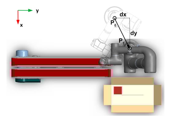
Figure 6.
Illustration of the result of optimising the location of the robot base position relative to the task space.
The robot path is implemented in three phases. In the first, a workpiece is picked up, which is then moved along a straight line perpendicular to the picking plane. In the second phase, movement takes place in the articulated space to a position above the drop point. In the third phase, the workpiece is lowered along a straight line to the put-down position. Between the phases, blending is carried out with a radius of 10 cm around the waypoints.
Maximum allowable velocities and accelerations are specified for each phase. For motion in task space, they are velocity and the linear acceleration of the TCP. For motion in the joint space, they are the velocities and accelerations of all joints. Based on these values and the developed position interpolators in both spaces, the robot path is designed, and the value of the cost function specific to the selected criterion for a given displacement of the robot via a given and is determined.
The velocity of the next particle and its position is then calculated, and this process is repeated iteratively until either the optimisation criterion is reached or a fixed population number is reached. The final result of the optimisation task is an indication of the components of the robot base displacement vector from point to the point providing the minimum of the defined objective function.
From a practical point of view, such an optimisation result is extremely useful for the robot operator, who, after inputting the coordinates of the pick-up and put-down points, obtains accurate information not only about the trajectory of the TCP, but also about the displacement of the robot by the vector [,] in order to perform the transport task optimised according to the selected criterion.
For each of the optimisation cases, a similar set of constraints was applied. In general, the optimisation criterion is defined as follows:
s.t.:
Objective function f is defined individually for each of the optimisation criteria.
4.1. Optimisation of the Duration of the Transport Task
Objective: Mono-criteria optimisation. The task is to determine the minimum transport cycle time.
The cycle time for the assumed constraints depends on the geometry and length of the TCP path. The path depends on how the robot is located relative to the task space and on the allowable constrains of velocities and accelerations in both spaces (inner and outer). The objective function will be further denoted as follows:
4.2. Optimisation of the Specific Energy Consumption
Objective: Mono-criteria optimisation. The task is to determine the minimum energy consumed to complete the transport cycle.
The energy required to move the workpiece along a given trajectory, according to the constraints, depends on the position, velocity and acceleration of the joints (18). The objective function will be further denoted as follows:
4.3. Optimisation of Economic Cost
Objective: Two-criteria optimisation. The task is to determine the minimum economic cost of completing a transport cycle taking into account both the energy and the workspace depreciation costs.
The optimisation objective has a strong economic rationale. An objective function has been constructed to implement this goal. It takes into account both the energy cost and the cost of extending the transport cycle lead time. Here, we will assume that the cost of completing a transport cycle (33) is decisively influenced by the cost of electric energy E and the depreciation cost of the robot P related to a single transport cycle.
The total increase in the cost of electric energy consumed per transport cycle relative to the minimum cost is:
where:
c—the cost per unit of electric energy;
—the electrical energy consumed per transport cycle;
—the minimum amount of electrical energy consumed per transport cycle.
The total increase in the depreciation cost of the workstation related to one transport cycle, which results from the increase in cycle time compared to the optimal solution, is:
where:
—the depreciation cost of the workstation related to the actual cycle time ;
—the minimum depreciation cost of the workstation;
—the total cost of depreciation of the workstation in units of payment (robot, mobile platform, conveyor, and equipment);
—the depreciation period;
—the actual cycle time;
—the minimum cycle time.
Finally, the cost function takes the form:
where:
; ; ; .
Since for a given robotic workstation, ultimately the economic cost function (36) is a linear combination of the electric energy consumed per transport cycle:
As can easily be seen, the cost function constructed in this way does not directly depend on the minimum value of the time and or the minimum specific energy. It therefore has an important application advantage as it does not require an a priori knowledge of both. Finally, the objective function will be further denoted as follows:
5. Case Study
5.1. ES5 Robot
To illustrate the proposed approach, let us consider the case of an industrial 6DoF articulated robot of type ES5 from EasyRobots [27]. The ES5 robot is a typical representative of the design line of articulated robots commonly used in industrial applications for pick-and-place operations. Figure 3 shows a three-dimensional drawing of this robot, together with the assigned right-hand local coordinate systems according to D-H representation. The D-H parameters of the ES5 robot are shown in Table 2.
Table 2.
Denavit–Hartenberg parameters for ES5 robot.
The solution of a forward kinematics for an ES5 robot, in the form of a transformation matrix is as follows:
while, the solution of the inverse kinematics is given in Equations (40)–(45).
where:
and are the x and y coordinates of the versor of the z axis.
Selected parameters of the electric motors and gears of the drive systems of each robot axis that are useful for the analytical model are shown in Table 1.
Table 3 shows the masses and the coordinates of the centres of mass of all robot links.
Table 3.
Masses and coordinates of the centres of gravity of the robot links.
5.2. Research Methodology
This section presents selected results from a research experiment, the main objective of which was the pointwise validation of the energy-efficient path planning approach for the 6DoF articulated robot. The following assumptions were made prior to the experiment:
- A quite typical variant of the transportation task was chosen. It imitates a typical pick-and-place task encountered in industrial practice;
- This variant relies on the movement of the workpiece from the pick-up point to the drop-off point, with a change in tool orientation between both positions. A graphical illustration of this task is shown in Figure 7.
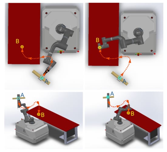 Figure 7. Graphical illustration of a transport task. The task relies on moving a piece, combined with the change of tool orientation. Symbols: A—pick-up point, B—put-down point.
The detailed technical parameters of a research experiment are given in Table 4.
Table 4.
Technological parameters of an experiment.
The aim of the research was to examine:
- The effectiveness of the developed approach in terms of searching for the optimal position of the robot in the -plane due to the minimisation of the specific cycle time;
- The effectiveness of the developed approach in terms of searching for the optimal position of the robot in the -plane of the task due to minimum energy consumption;
- The effectiveness of the developed approach in terms of searching for the optimal position of the robot in the -plane of the task, due to a mixed criterion imposing a penalty on the cycle execution time and rewarding the savings of the energy expenditures necessary for its execution. In this case, the coefficients and (37) are calculated based on the parameters given in Table 5.
Table 5. Economic parameters of a research experiment.
5.3. Test Bench
A series of validation experiments were executed at a laboratory test bench (Figure 8), consisting of an ES5 robot equipped with a two-jaw gripper and mounted on an AMR mobile platform manufactured by UVC-MED company [48].
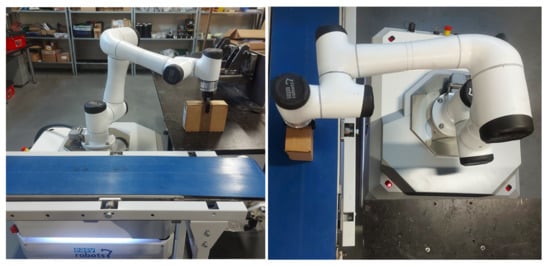
Figure 8.
Six-degrees-of-freedom articulated ES5 robot and autonomous mobile platform.
Measurements of the instantaneous power consumption of the electric motors driving the robot joints were performed via the functionality of the drive controllers. The instantaneous current consumption and supply voltage samples were transmitted from the drive controllers to the industrial computer using the EtherCAT serial industrial communication network. The ES5 robot is equipped with miControl E55 controllers [49] responsible for controlling joints 1–3 and E65 series controllers [50] controlling joints 4–6. Voltages and currents drawn by all of the drives of all robots’ motors were sampled and acquired every 20 ms. Figure 9 shows the basic components of the measuring system used in experiments.
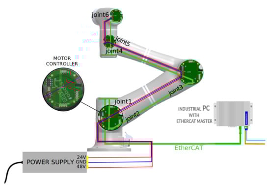
Figure 9.
Graphic diagram of the basic components of the measuring system.
6. Research Experiment
6.1. Verification of the Analytical Model of Specific Energy Consumption
Research objective: Experimental, point-wise assessment of the quality of the analytical model of a specific energy consumption.
Experimental verification of the analytical model of the specific energy consumption was performed using a test bench presented in Section 5.3. The bench allows for the measurement and acquisition of the currents and voltages of all robot’s motors in on-line mode. On this basis, already in off-line mode, the values of instantaneous power and total energy consumed for the transport task were determined. The exemplary results of the experimental verification of the model output for each of the six robot axes are shown in Figure 10. The reference value used for the estimation of the relative modelling errors are the nominal powers of the robot’s motors.
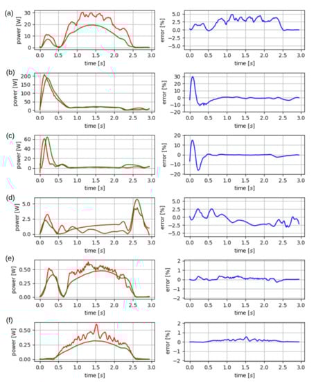
Figure 10.
Results of the experimental verification of the specific energy consumption. The charts (a–f) show the instantaneous power consumption of all six robot’s motors. The green plot indicates instantaneous power of the model output; red plot indicates experimentally measured instantaneous power. Blue plot indicates the relative modelling error.
Based on the graph depicted in Figure 10, it can be assessed that the developed model correctly tracks the trend of the power consumption. In the some regions of the plots given in Figure 10, there are visible inaccuracies in the model. In part, this results from the simplifications made, which are described in Section 3.1.2. The calculations based on (21) show that the use of the model, despite the modelling errors, gives quite as good results by determining the total power consumption (Table 6 and Table 7). Therefore, this may confirm to some extent the validity of the model.
Table 6.
Comparison of the specific energy modelled and measured for each axis.
Table 7.
Comparison of the total modelled and total measured energy for 8 random trajectories.
6.2. Minimisation of Transport Cycle Time
Research objective: To investigate the relationship between cycle time and the robot base location.
The optimisation task was performed using a meta-heuristic 40-particle swarm algorithm implemented in a sequence of 20 iterations. The minimum cycle time and the specific energy required to complete the cycle for the three optimisation criteria are searched:
- The minimum cycle time;
- The minimum energy consumed;
- The minimum economic cost.
The average specific energy consumption was examined for 900 equidistant positions of the robot base in the -plane. The location points were distributed uniformly in a grid with a raster of mm. The obtained results are shown in Table 8 and in Figure 11.
Table 8.
Results of optimisation tasks.
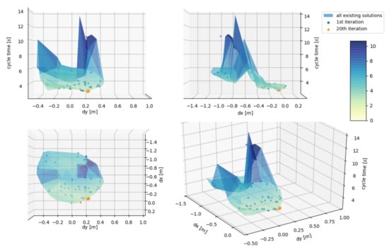
Figure 11.
Specific cycle time in terms of the displacement vector of the robot base [dx,dy].
6.3. Minimisation of Specific Energy Consumption
Research objective: To investigate the relationship between the energy required to complete one transport cycle and location of the robot base.
Similarly as in Section 6.2, the optimisation task was performed using a meta-heuristic 40-particle swarm algorithm. The obtained numerical results of minimal values for the energy of single transport cycle are presented in Table 9. In addition, the averaged values of specific energy, cycle execution time and the displacement vector of the robot base are presented in the last column of Table 9.
Table 9.
Results of minimisation of specific energy consumption.
The average power consumption of the same transport task for the robot location at the all nodes of the grid is equal to 134.27 J. Hence, in the analysed case, an appropriate choice of robot location could result in energy savings of up to 48.9%. Such a high degree of expected savings in specific energy is a strong argument for implementing the proposed approach in industrial practice. Figure 12 shows plots of the specific energy in relation to the components of the robot base displacement vector.
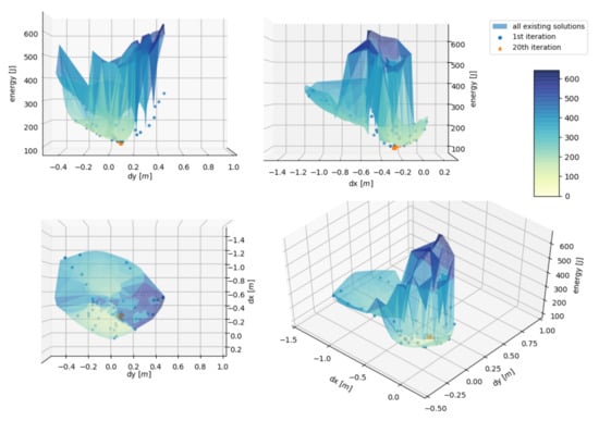
Figure 12.
Specific energy in terms of the displacement vector of the robot base [dx,dy].
6.4. Minimisation of the Economic Cost
Task objective: To investigate the relationship between the economic cost of executing a single transportation cycle and the location of the robot base.
According to the optimisation criterion (38), the economic cost of the single transport operation, consisting of the workspace depreciation and energy consumption costs, was analysed. The economic parameters used for this research are shown in Table 5. Similar to the Section 6.2 and Section 6.3, the optimisation task was carried out using the 40-particle swarm metaheuristic algorithm. The optimisation task was carried out in 20 iterations. The obtained numerical results are shown in Table 10. For comparison goals, the values of the specific energy of the transport cycle for different optimisation criteria are also presented in this table.
Table 10.
Results for minimisation of economic cost of single transport cycle.
The specific transport cost versus displacement vector components of the robot base is shown in Figure 13.
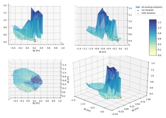
Figure 13.
Specific transport cost [USD] in terms of the displacement vector of the robot base [dx,dy].
7. Discussion
A discussion of the results will be presented in accordance with the experiment results reported in Section 6.
7.1. Verification of the Analytical Model of Specific Energy Consumption
The analytical model output was found to converge with the measurements. The maximum differences between the total measured and modelled energy values do not exceed 9.8%. This may be assumed as an acceptable result, taking into account the undertaken simplifications and concerning, in particular, nonlinear phenomena, the uncertainty of identification of the model parameters and the uncertainty of the measurements. The model is applicable, because the predicted energy savings are almost one order higher in magnitude than model inaccuracy. Hence, it should be considered that the analytical model shows potentially beneficial performance characteristics.
It is, of course, possible to derive higher-fidelity models based on experimental data and using computational techniques. However, data-driven models are impractical in the context of implementing optimisation tasks. This is because, unlike the proposed approach, they require expensive and labour-intensive preliminary studies.
7.2. Minimisation of Transport Cycle Time
Analysing the experimental results of the time minimisation study, we can draw the following three qualitative conclusions:
- The robot base location has a significant impact on both the cycle time and the energy expenditure required to complete the cycle;
- The criterion that optimises cycle time is inefficient from an energy point of view in the sense that even a small increase in this time allows for significant savings in energy consumption;
- In the absence of an upper limit on cycle time, a mixed optimisation criterion should be used.
7.3. Minimisation of the Specific Energy Consumption
By analysing the results of optimisation and experimental studies on the minimisation of specific energy consumption, we can draw the following qualitative conclusions:
- The choice of the location of the robot base relative to the task space has a significant impact on the value of specific energy consumption;
- The optimising specific energy consumption is recommended to be used before the searching for a minimum cycle time. Significant energy savings can be achieved at the expense of a small increase in cycle time.
In the case study analysed, the appropriate selection of the robot base location could result in savings of up to 48.9%. Such a high level of expected savings in specific energy consumption is a strong argument for implementing the proposed energy optimisation solution in industrial practice.
7.4. Minimisation of the Economic Cost
Minimising the economic cost is a rational postulate and, moreover, one that is desirable and acceptable from the point of view of the economics of production processes. Therefore, the economic cost minimisation should be considered as the primary criterion. As demonstrated in the case study, it is possible to achieve the minimum economic cost of a transport task with only a slight drop in productivity.
7.5. Comparison of the Achieved Results
The use of the energy minimisation criterion alone will not yield satisfactory results having a negative impact on the cycle time (Table 8). In the case studied, the cycle time obtained by energy minimisation is 36.3% worse than via the time minimisation criterion. For process efficiency, this is a significant deterioration. The situation is similar for the case of cycle time minimisation, in which the energy consumed has increased by almost 150% compared to the energy minimisation case. This makes it reasonable to use a multi-criteria optimisation. This was achieved by designing a minimum economic cost function. This resulted in a deterioration of the minimum time by only 2.8% relative to the time-optimal case, and in 41.8% increase in the value of energy consumption relative to the energy-optimal case. By minimising the economic cost of a single transport cycle, we can expect savings of up to 8% compared to the minimum energy case, and up to 3.5% compared to the minimum cycle time case.
8. Conclusions
The ultimate goal of the reported applied research was to solve a real-world technical and economical problem of the rational planning of pick-and-place operations signalled by one of the industrial robot companies.
We proposed a multi-objective, proven, and easy to implement solution to this problem that allows for energy savings on the one hand, and an increase in the productivity of the pick-and-place operations on the other.
The proposed approach makes it possible to support the human operator in the rational choice of robot’s location in the workspace. In this sense, the approach has a clear application aspect.
The basic technical problem identified and solved in this paper concerns the automated support of the setting up of articulated robots for the efficient execution of pick-and-place transport tasks. The proposed solution allows for the automated planning of the path, trajectory, TCP transition function, and location of the robot in the workstation space.
The presented approach is systematic and innovative. It proposes a well-defined three-step solution to the problem at a sufficiently high level of generality. It also has the characteristics of a scalable solution, as the developed model can be applied to the industrial robots with different number of degrees of freedom.
It is also worth highlighting that, in the context of rising energy prices, the proposal for an energy-efficient approach to planning pick-and-place operations takes on particular importance.
In the near future, it is planned to develop the approach that also takes into account the issue of durability of harmonic gears used in the drive systems of robot joints.
Author Contributions
Conceptualisation, M.B. and Ł.G.; methodology M.B. and Ł.G.; software Ł.G.; validation, Ł.G.; formal analysis, Ł.G.; investigation, Ł.G.; resources, Ł.G.; data curation, Ł.G.; writing—original draft preparation M.B. and Ł.G.; writing—review and editing, M.B. and Ł.G.; visualisation, Ł.G.; supervision, M.B.; project administration, Ł.G.; funding acquisition, M.B. All authors have read and agreed to the published version of the manuscript.
Funding
Institute of Automation and Robotics of the Warsaw University of Technology within the framework of statutory research activities.
Data Availability Statement
Not applicable.
Conflicts of Interest
The authors declare no conflict of interest.
References
- IFR World Robotics 2021 Reports. Available online: https://ifr.org/ifr-press-releases/news/robot-sales-rise-again (accessed on 23 August 2022).
- Zhou, G.; Luo, J.; Li, R.; Xiang, K.; Xu, S.; Pang, M.; Tang, B.; Zhang, S. A framework of industrial operations for hybrid robots. In Proceedings of the 2021 26th International Conference on Automation and Computing (ICAC), Portsmouth, UK, 2–4 September 2021; pp. 1–6. [Google Scholar] [CrossRef]
- Mohammadpour, M.; Zeghmi, L.; Kelouwani, S.; Gaudreau, M.A.; Amamou, A.; Graba, M. An Investigation into the Energy-Efficient Motion of Autonomous Wheeled Mobile Robots. Energies 2021, 14, 3517. [Google Scholar] [CrossRef]
- Ratiu, M.; Prichici, M. Industrial robot trajectory optimization—A review. MATEC Web Conf. 2017, 126, 02005. [Google Scholar] [CrossRef]
- Bartyś, M.; Hryniewicki, B. The Trade-Off between the Controller Effort and Control Quality on Example of an Electro-Pneumatic Final Control Element. Actuators 2019, 8, 23. [Google Scholar] [CrossRef]
- Mitrevski, A.; Abdelrahman, A.; N J, A.; Plöger, P. On the Diagnosability of Actions Performed by Contemporary Robotic Systems *. In Proceedings of the 31st International Workshop on Principles of Diagnosis: DX-2020, Nashville, TN, USA, 26–28 September 2020. [Google Scholar]
- Rymansaib, Z.; Iravani, P.; Sahinkaya, M. Exponential trajectory generation for point to point motions. In Proceedings of the 2013 IEEE/ASME International Conference on Advanced Intelligent Mechatronics, Wollongong, Australia, 9–12 July 2013; pp. 906–911. [Google Scholar] [CrossRef]
- Carabin, G.; Wehrle, E.; Vidoni, R. A Review on Energy-Saving Optimization Methods for Robotic and Automatic Systems. Robotics 2017, 6, 39. [Google Scholar] [CrossRef]
- Li, Y.; Bone, G. Are parallel manipulators more energy efficient? In Proceedings of the 2001 IEEE International Symposium on Computational Intelligence in Robotics and Automation (Cat. No.01EX515), Banff, AB, Canada, 29 July–1 August 2001; pp. 41–46. [Google Scholar] [CrossRef]
- Kim, Y.J. Design of low inertia manipulator with high stiffness and strength using tension amplifying mechanisms. In Proceedings of the 2015 IEEE/RSJ International Conference on Intelligent Robots and Systems (IROS), Hamburg, Germany, 28 September–3 October 2015; pp. 5850–5856. [Google Scholar] [CrossRef]
- Yin, H.; Liu, J.; Yang, F. Hybrid Structure Design of Lightweight Robotic Arms Based on Carbon Fiber Reinforced Plastic and Aluminum Alloy. IEEE Access 2019, 7, 64932–64945. [Google Scholar] [CrossRef]
- Boscariol, P.; Gallina, P.; Gasparetto, A.; Giovagnoni, M.; Scalera, L.; Vidoni, R. Evolution of a Dynamic Model for Flexible Multibody Systems. Adv. Ital. Mech. Sci. 2016, 47, 533–541. [Google Scholar] [CrossRef]
- Vidoni, R.; Scalera, L.; Gasparetto, A. 3-D ERLS based dynamic formulation for flexible-link robots: Theoretical and numerical comparison between the finite element method and the component mode synthesis approaches. Int. J. Mech. Control 2018, 19, 39–50. [Google Scholar]
- Carabin, G.; Palomba, I.; Wehrle, E.; Vidoni, R. Energy Expenditure Minimization for a Delta-2 Robot Through a Mixed Approach. In Proceedings of the Multibody Dynamics 2019; Kecskeméthy, A., Geu Flores, F., Eds.; Springer International Publishing: Cham, Switzerland, 2020; pp. 383–390. [Google Scholar] [CrossRef]
- Barreto, J.P.; Corves, B. Resonant Delta Robot for Pick-and-Place Operations. In Advances in Mechanism and Machine Science; Uhl, T., Ed.; Springer International Publishing: Cham, Switzerland, 2019; pp. 2309–2318. [Google Scholar] [CrossRef]
- Scalera, L.; Carabin, G.; Vidoni, R.; Wongratanaphisan, T. Energy efficiency in a 4-DOF parallel robot featuring compliant elements. Int. J. Mech. Control 2019, 20, 49–57. [Google Scholar]
- Ruiz, A.G.; Fontes, J.; Silva, M. The Influence Of Kinematic Redundancies In The Energy Efficiency Of Planar Parallel Manipulators. In Proceedings of the ASME 2015 International Mechanical Engineering Congress and Exposition IMECE2015, Houston, TX, USA, 13–19 November 2015. [Google Scholar] [CrossRef]
- Boscariol, P.; Richiedei, D. Trajectory Design for Energy Savings in Redundant Robotic Cells. Robotics 2019, 8, 15. [Google Scholar] [CrossRef]
- Atef; Salami, M.; Johar, H. Optimum Joint Profilefor Constrained Motionofa Planar Rigid-Flexible Manipulator. In Proceedings of the 19th International Conference on CAD/CAM Robotic and Factories of the Future CARs &FOF, Kuala Lumpur, Malaysia, 22–24 July 2003. [Google Scholar]
- Zlajpah, L. On time optimal path control of manipulators with bounded joint velocities and torques. In Proceedings of the IEEE International Conference on Robotics and Automation, Minneapolis, MI, USA, 22–28 April 1996; Volume 2, pp. 1572–1577. [Google Scholar] [CrossRef]
- Hansen, C.; Oltjen, J.; Meike, D.; Ortmaier, T. Enhanced approach for energy-efficient trajectory generation of industrial robots. In Proceedings of the 2012 IEEE International Conference on Automation Science and Engineering (CASE 2012), Los Alamitos, CA, USA, 20–24 August 2012; pp. 1–7. [Google Scholar] [CrossRef]
- Belaïd Dlimi, I.; Kallel, H. Optimal neural control for constrained robotic manipulators. In Proceedings of the 2010 5th IEEE International Conference Intelligent Systems, London, UK, 7–9 July 2010; pp. 302–308. [Google Scholar] [CrossRef]
- Pérez Bailón, W.; Barrera Cardiel, E.; Juárez Campos, I.; Ramos Paz, A. Mechanical energy optimization in trajectory planning for six DOF robot manipulators based on eighth-degree polynomial functions and a genetic algorithm. In Proceedings of the 2010 7th International Conference on Electrical Engineering Computing Science and Automatic Control, 8–10 September 2010; pp. 446–451. [Google Scholar] [CrossRef]
- UR5 Technical Specifications. Available online: https://www.universal-robots.com/media/50588/ur5_en.pdf (accessed on 23 August 2022).
- YuMi-IRB 14000, Collaborative Robot. Available online: https://new.abb.com/products/robotics/collaborative-robots/irb-14000-yumi (accessed on 23 August 2022).
- KUKA-LBR-iiwa Technical Data. Available online: https://www.reeco.co.uk/wp-content/uploads/2020/05/KUKA-LBR-iiwa-technical-data.pdf (accessed on 23 August 2022).
- ES5 Robot Technical Specification. Available online: https://easyrobots.pl/en/roboty-przemyslowe-es5 (accessed on 23 August 2022).
- Hofmann, D.C.; Polit-Casillas, R.; Roberts, S.N.; Borgonia, J.P.; Dillon, R.P.; Hilgemann, E.; Kolodziejska, J.; Montemayor, L.; Suh, J.-o.; Hoff, A.; et al. Castable Bulk Metallic Glass Strain Wave Gears: Towards Decreasing the Cost of High-Performance Robotics. Sci. Rep. 2016, 6, 37773. [Google Scholar] [CrossRef] [PubMed]
- Paes, K.; Dewulf, W.; Elst, K.; Kellens, K.; Slaets, P. Energy Efficient Trajectories for an Industrial ABB Robot. Procedia CIRP 2014, 15, 105–110. [Google Scholar] [CrossRef]
- Boscariol, P.; Caracciolo, R.; Richiedei, D.; Trevisani, A. Energy Optimization of Functionally Redundant Robots through Motion Design. Appl. Sci. 2020, 10, 3022. [Google Scholar] [CrossRef]
- Meike, D.; Pellicciari, M.; Berselli, G. Energy Efficient Use of Multirobot Production Lines in the Automotive Industry: Detailed System Modeling and Optimization. Autom. Sci. Eng. IEEE Trans. 2014, 11, 798–809. [Google Scholar] [CrossRef]
- Meike, D.; Pellicciari, M.; Berselli, G.; Vergnano, A.; Ribickis, L. Increasing the energy efficiency of multi-robot production lines in the automotive industry. In Proceedings of the 2012 IEEE International Conference on Automation Science and Engineering (CASE), Seoul, Republic of Korea, 20–24 August 2012; pp. 700–705. [Google Scholar] [CrossRef]
- Li, X.; Lan, Y.; Jiang, P.; Cao, H.; Zhou, J. An Efficient Computation for Energy Optimization of Robot Trajectory. IEEE Trans. Ind. Electron. 2022, 69, 11436–11446. [Google Scholar] [CrossRef]
- Feddema, J. Kinematically optimal robot placement for minimum time coordinated motion. In Proceedings of the IEEE International Conference on Robotics and Automation, Minneapolis, MN, USA, 22–28 April 1996; Volume 4, pp. 3395–3400. [Google Scholar] [CrossRef]
- Spensieri, D.; Carlson, J.S.; Bohlin, R.; Kressin, J.; Shi, J. Optimal Robot Placement for Tasks Execution. Procedia CIRP 2016, 44, 395–400. [Google Scholar] [CrossRef]
- Hwang, Y.K.; Watterberg, P. Optimizing Robot Placement for Visit-Point Tasks; Sandia National Laboratories: Albuquerque, NM, USA, 1996; Available online: https://digital.library.unt.edu/ark:/67531/metadc672157 (accessed on 23 August 2022).
- Vysocký, A.; Papřok, R.; Šafařík, J.; Kot, T.; Bobovský, Z.; Novák, P.; Snášel, V. Reduction in Robotic Arm Energy Consumption by Particle Swarm Optimization. Appl. Sci. 2020, 10, 8241. [Google Scholar] [CrossRef]
- Zhang, M.; Yan, J. A data-driven method for optimizing the energy consumption of industrial robots. J. Clean. Prod. 2021, 285, 124862. [Google Scholar] [CrossRef]
- Rajan, V. Minimum time trajectory planning. In Proceedings of the 1985 IEEE International Conference on Robotics and Automation, St. Louis, MI, USA, 25–28 March 1985; Volume 2, pp. 759–764. [Google Scholar] [CrossRef]
- Verscheure, D.; Demeulenaere, B.; Swevers, J.; De Schutter, J.; Diehl, M. Time-Optimal Path Tracking for Robots: A Convex Optimization Approach. IEEE Trans. Autom. Control 2009, 54, 2318–2327. [Google Scholar] [CrossRef]
- Švejda, M.; Čechura, T. Interpolation method for robot trajectory planning. In Proceedings of the 2015 20th International Conference on Process Control (PC), Strbske Pleso, Slovakia, 9–12 June 2015; pp. 406–411. [Google Scholar] [CrossRef]
- Volpe, R. Task space velocity blending for real-time trajectory generation. In Proceedings of the [1993] Proceedings IEEE International Conference on Robotics and Automation, Atlanta, GA, USA, 2–6 May 1993; Volume 2, pp. 680–687. [Google Scholar] [CrossRef]
- Kennedy, J.; Eberhart, R. Particle swarm optimization. In Proceedings of the ICNN’95—International Conference on Neural Networks, Perth, WA, Australia, 27 November–1 December 1995; Volume 4, pp. 1942–1948. [Google Scholar] [CrossRef]
- Craig, J.J. Introduction to Robotics: Mechanics and Control, 2nd ed.; Addison-Wesley Longman Publishing Co., Inc.: Boston, MA, USA, 1989. [Google Scholar] [CrossRef]
- Hawkins, K.P. Analytic Inverse Kinematics for the Universal Robots UR-5/UR-10 Arms. In Georgia Tech Library; Technical report; Georgia Institute of Technology: Atlanta, GA, USA.
- Spong, M.W. Robot Dynamics and Control, 1st ed.; John Wiley & Sons, Inc.: Hoboken, NJ, USA, 1989. [Google Scholar] [CrossRef]
- Nidec Shimpo Flexwave WP Series Brochure. Available online: http://www.drives.nidec-shimpo.com/wp-content/uploads/2021/12/FLEXWAVE_Brochure40930N.pdf (accessed on 23 August 2022).
- AMR Robot Technical Specification. Available online: https://uvc-med.pl/robotower/ (accessed on 23 August 2022).
- MiControl E55 Brochure. Available online: https://www.micontrol.de/en/products/devices/mcdsa-e55 (accessed on 23 August 2022).
- MiControl E55 Brochure. Available online: https://www.micontrol.de/en/products/devices/mcdsa-e65-modul (accessed on 23 August 2022).


Publisher’s Note: MDPI stays neutral with regard to jurisdictional claims in published maps and institutional affiliations. |
© 2022 by the authors. Licensee MDPI, Basel, Switzerland. This article is an open access article distributed under the terms and conditions of the Creative Commons Attribution (CC BY) license (https://creativecommons.org/licenses/by/4.0/).