
Diagnosing Disk-Space Variation in Distribution Power Transformer Windings Using Group Method of Data Handling Artificial Neural Networks


Abstract
:1. Introduction
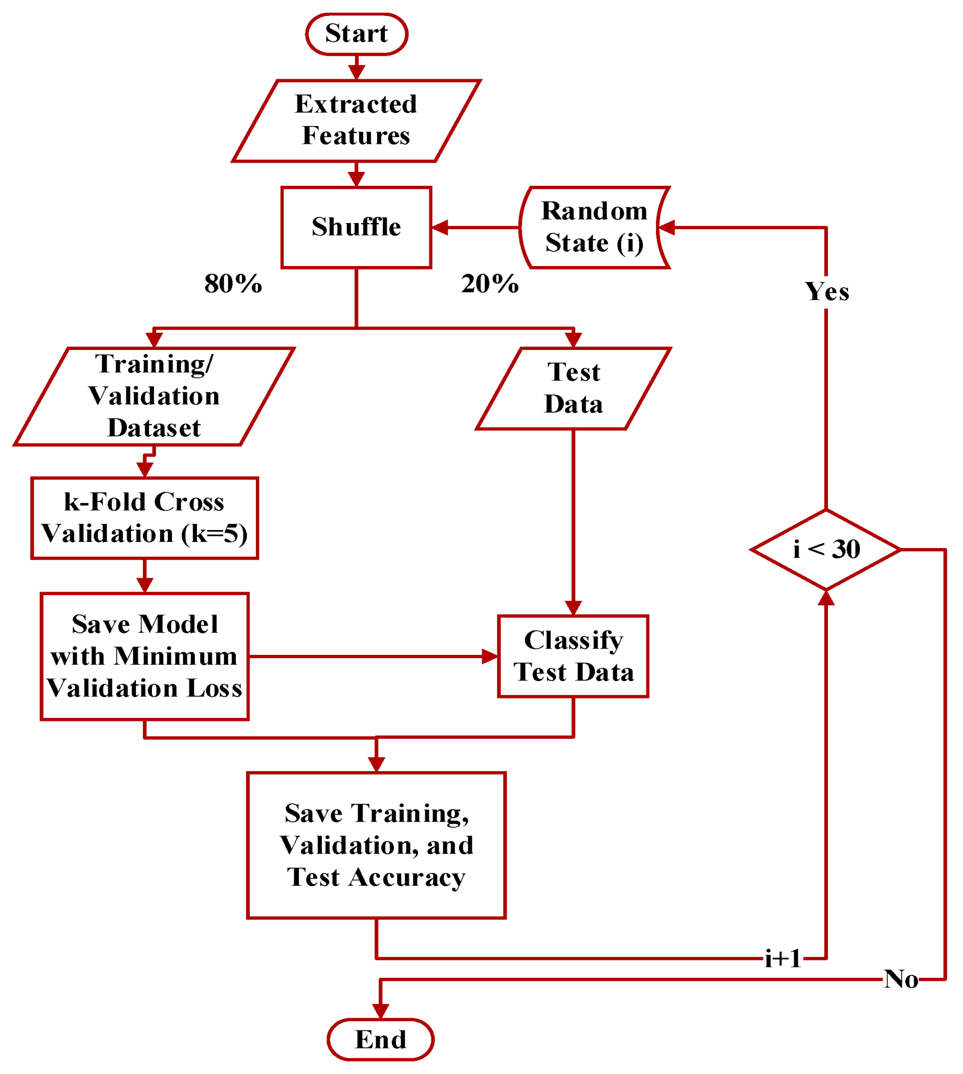
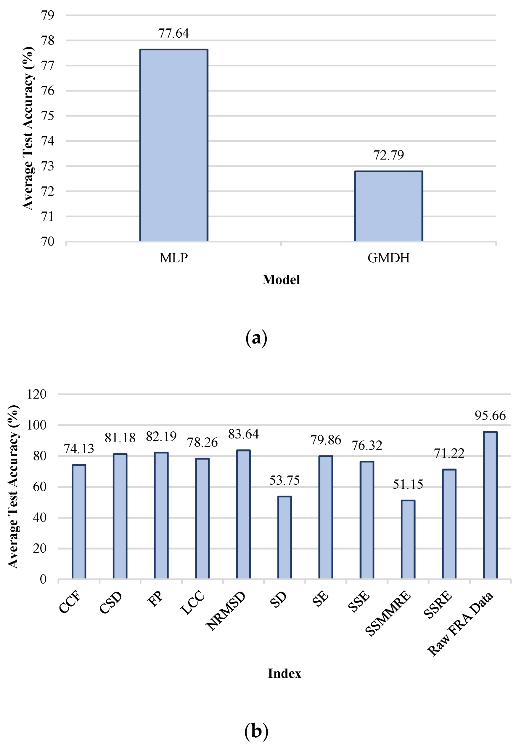
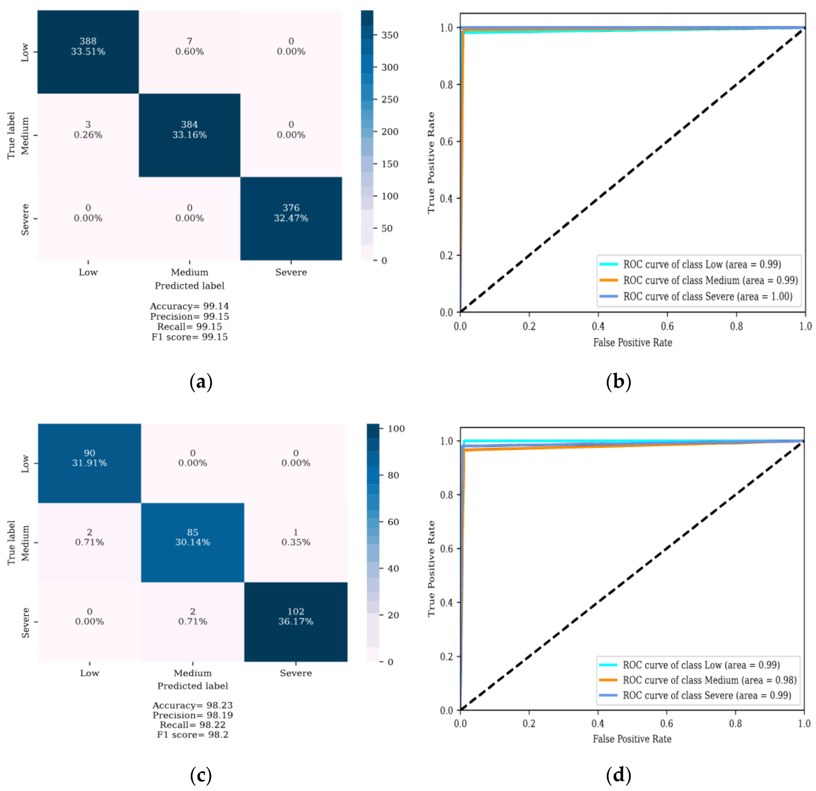
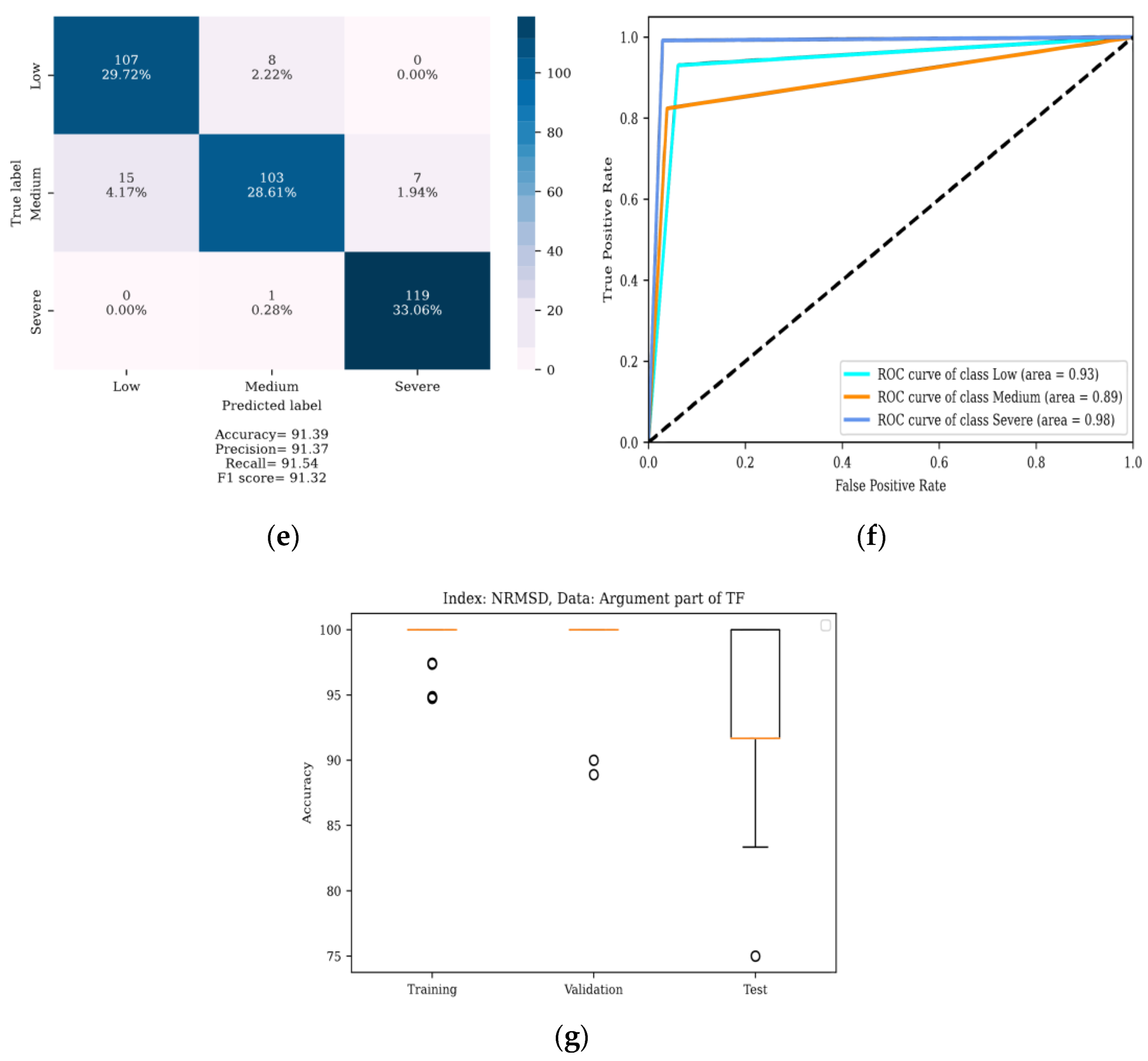
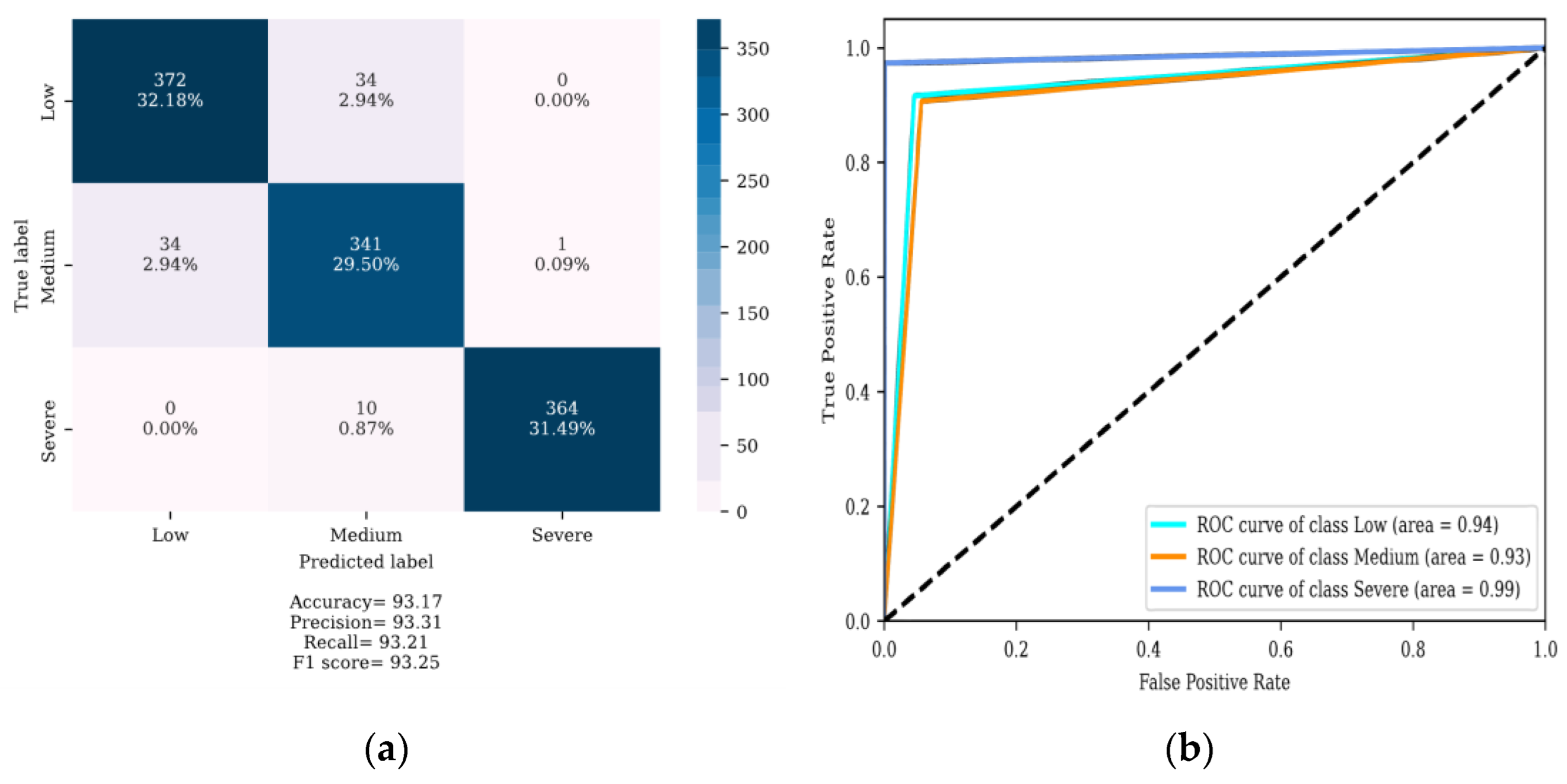
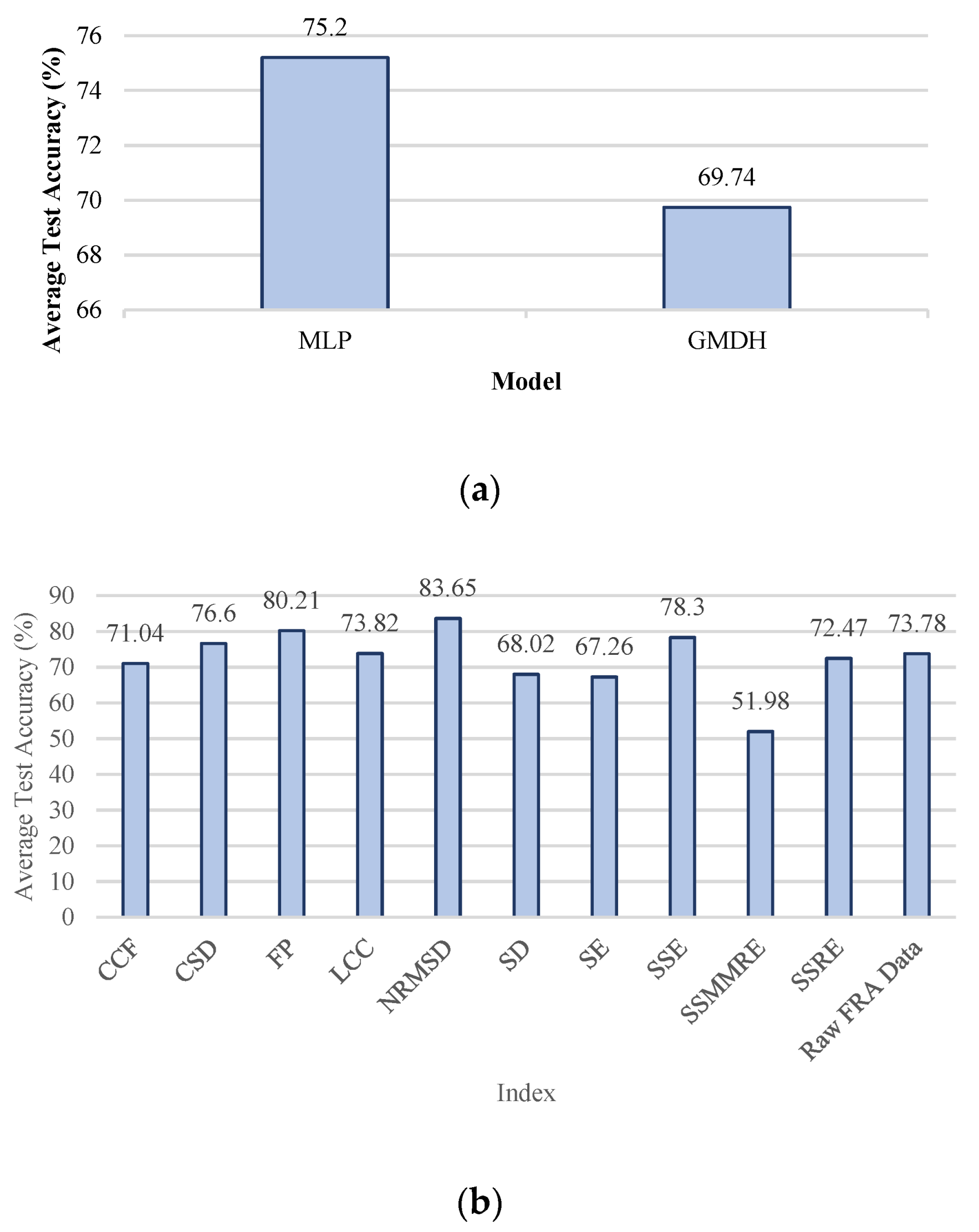
- A new AI-based interpreter of the TF test results has been proposed. A GMDH artificial neural network has been employed to determine the severity and location of DSV faults. The results of classification using GMDH have been compared to the results of the MLP neural network. In order to assess the performance of the intelligent classifiers, a well-known method called k-fold cross validation has been utilized;
- At the feature extraction stage, ten appropriate NIns used to extract feature groups to feed the proposed intelligent fault detectors;
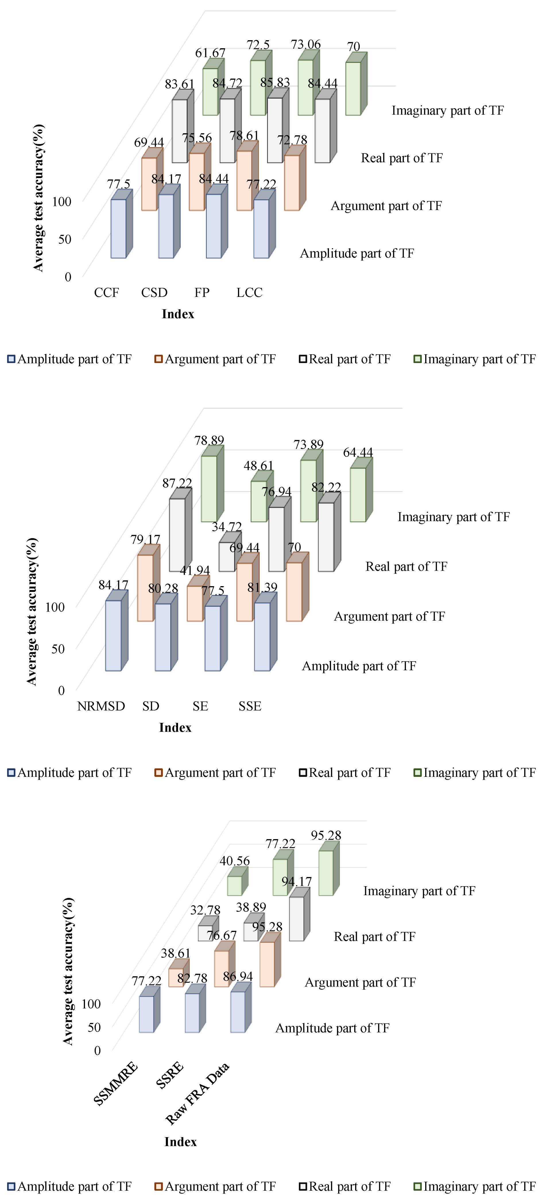
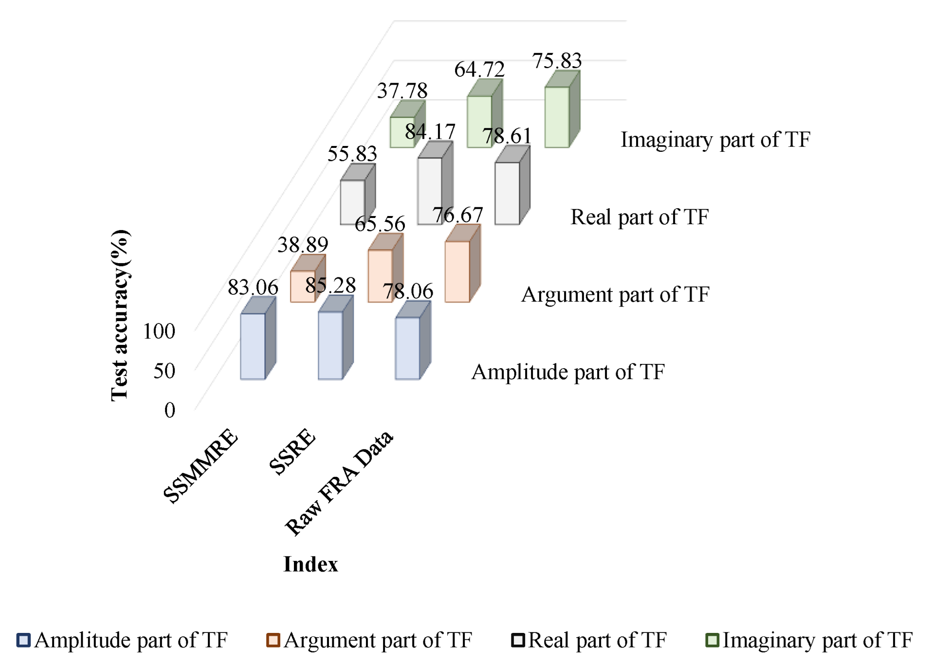
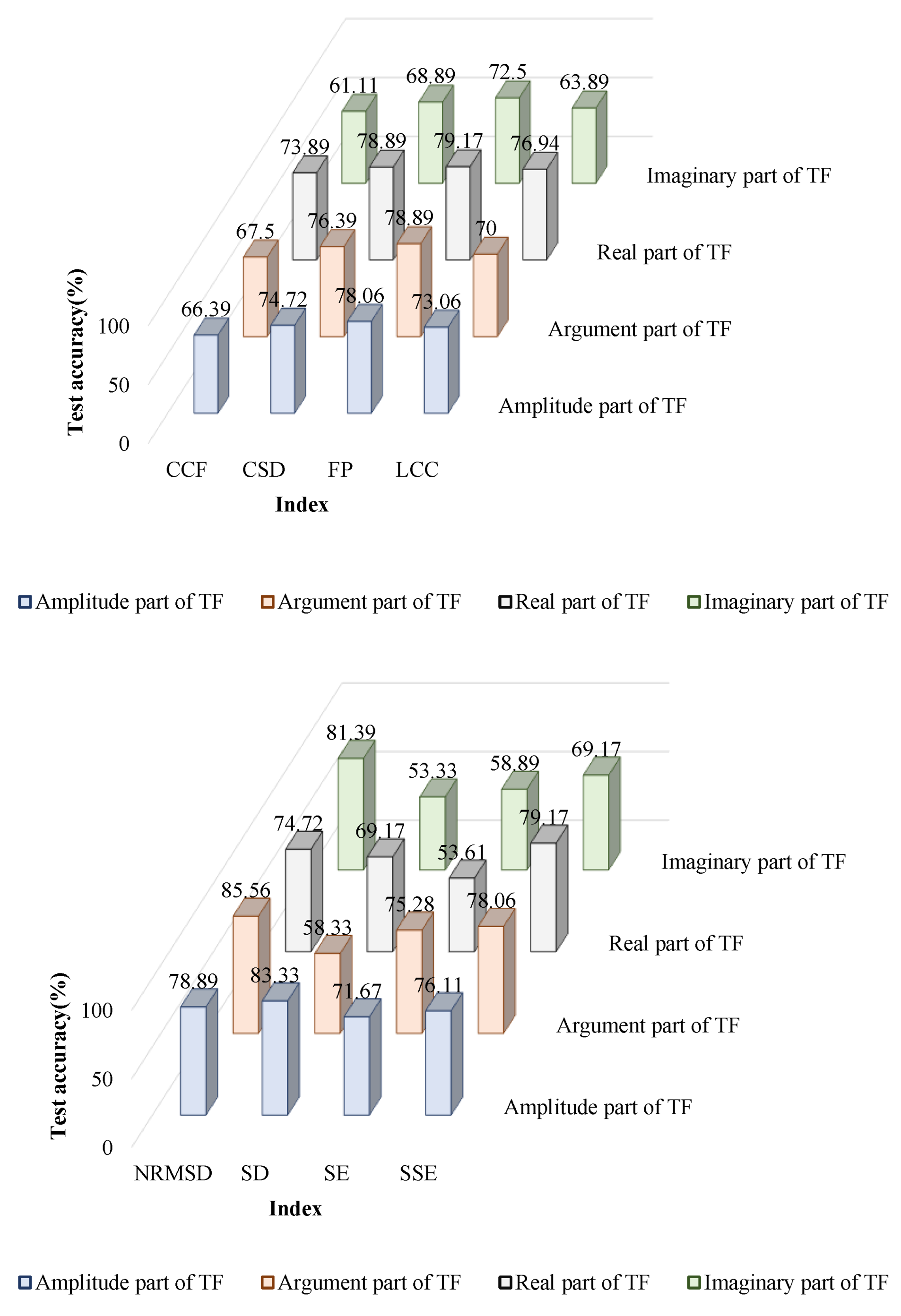
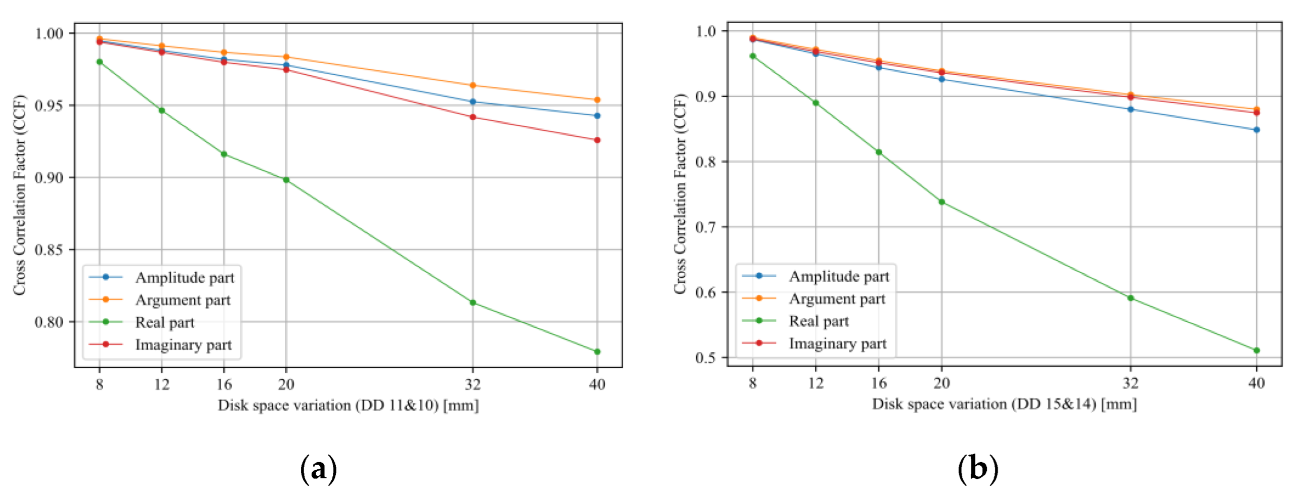
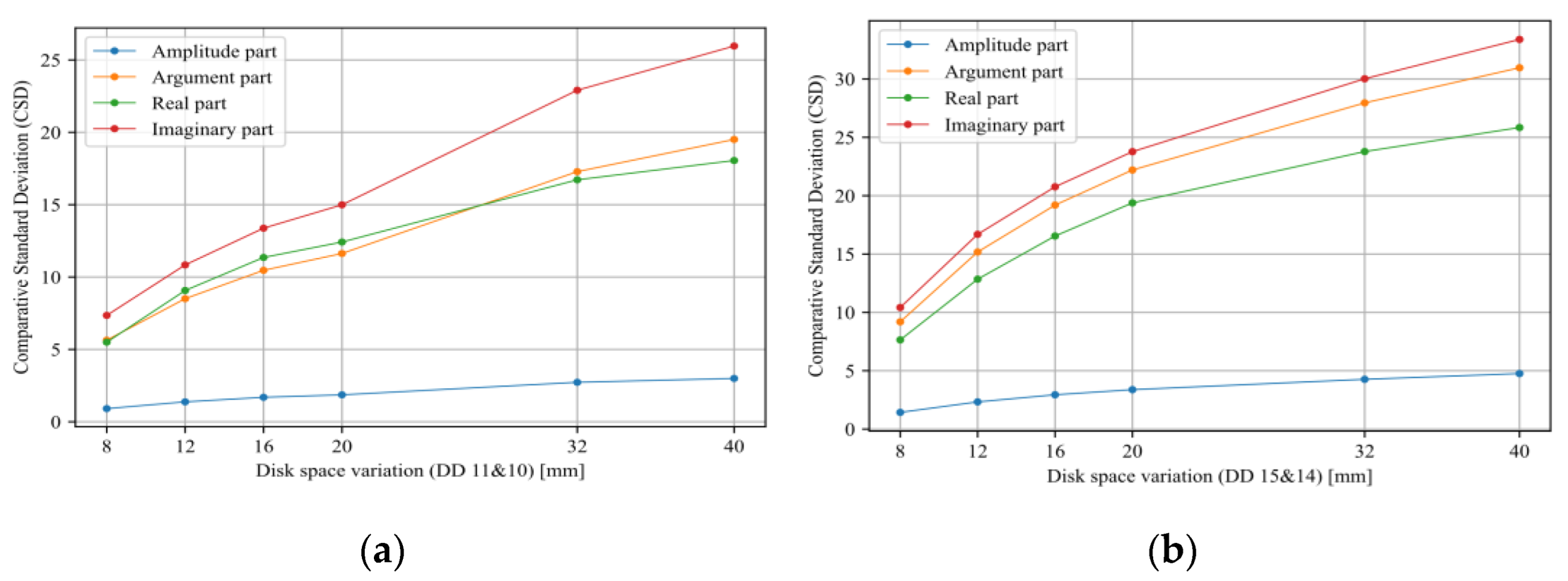
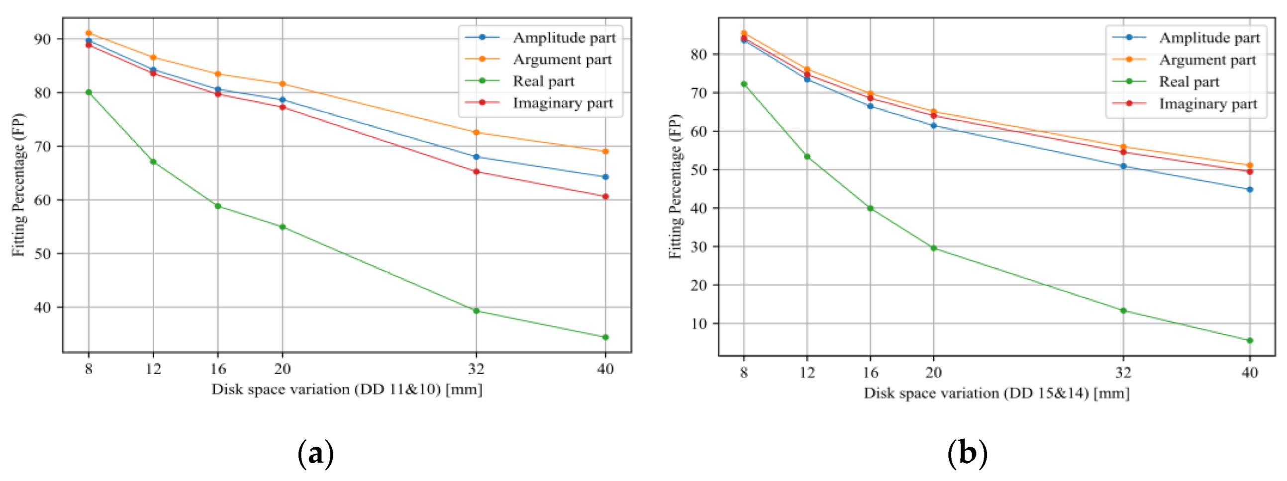
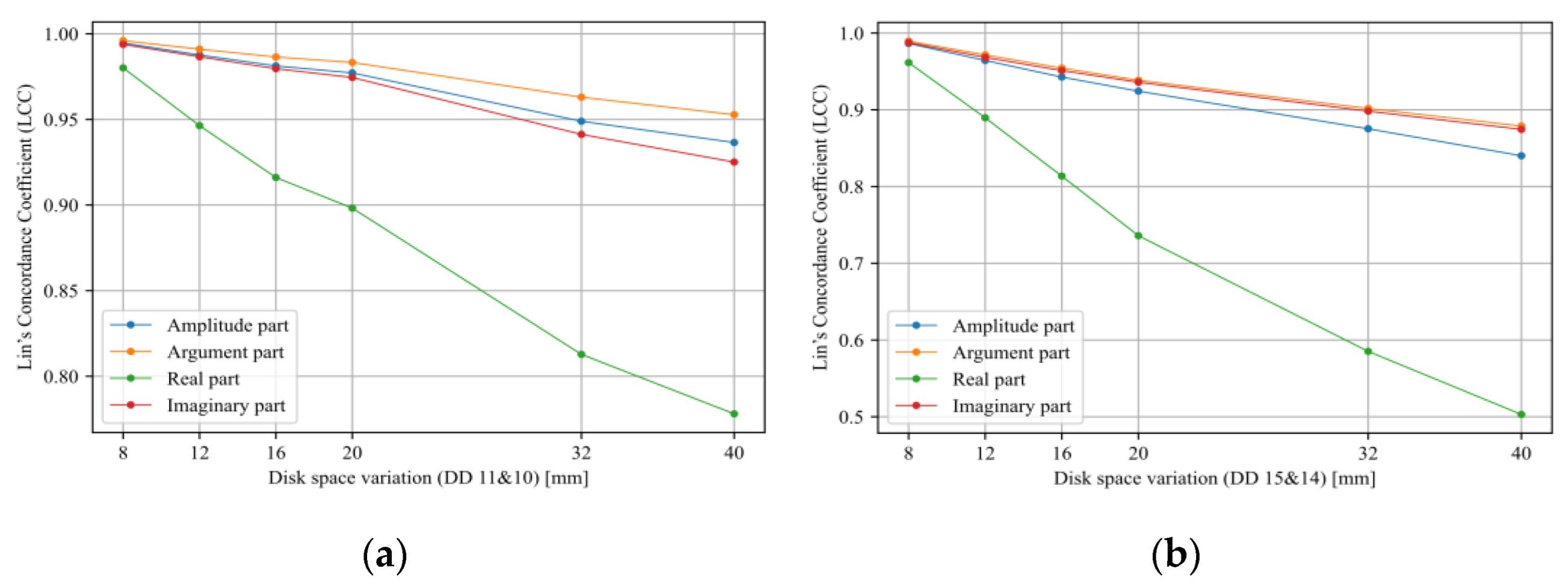
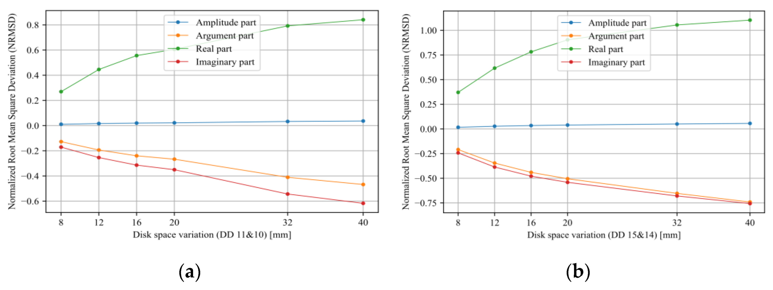
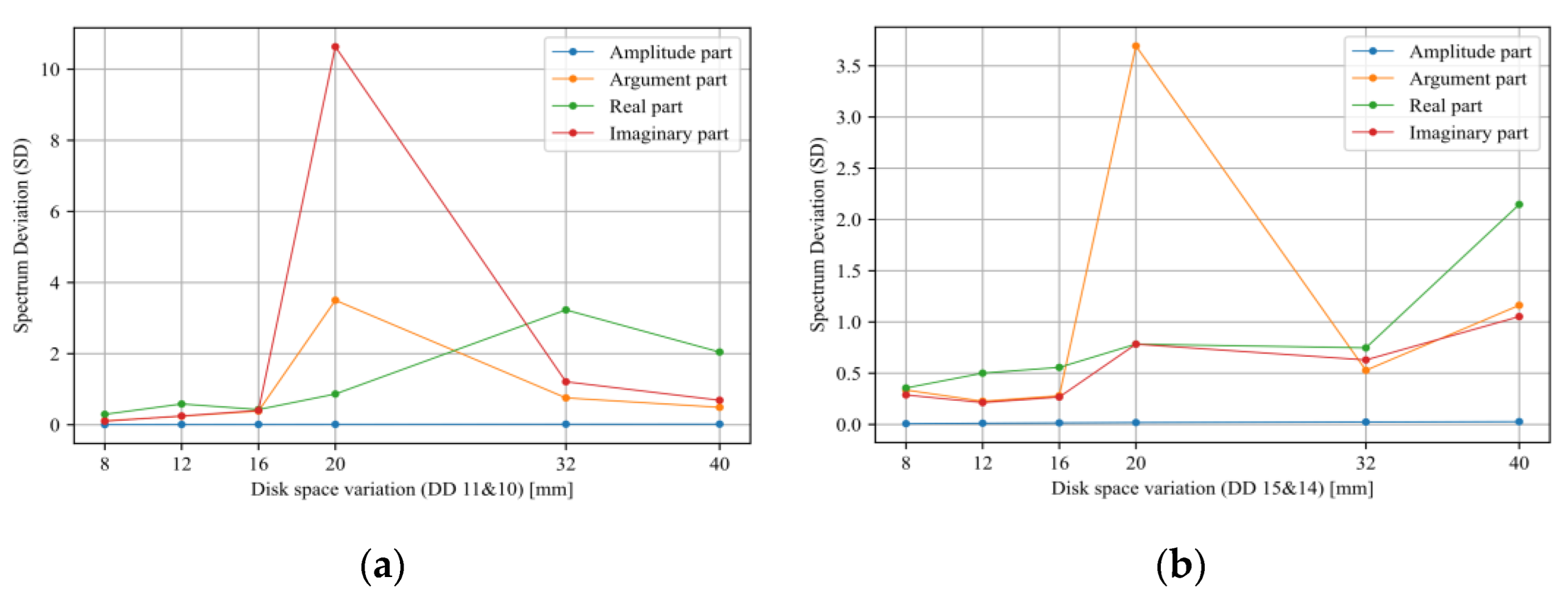
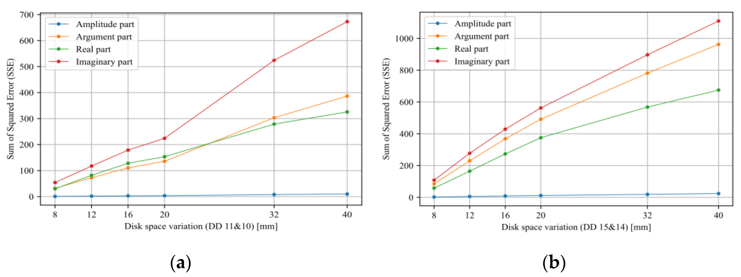
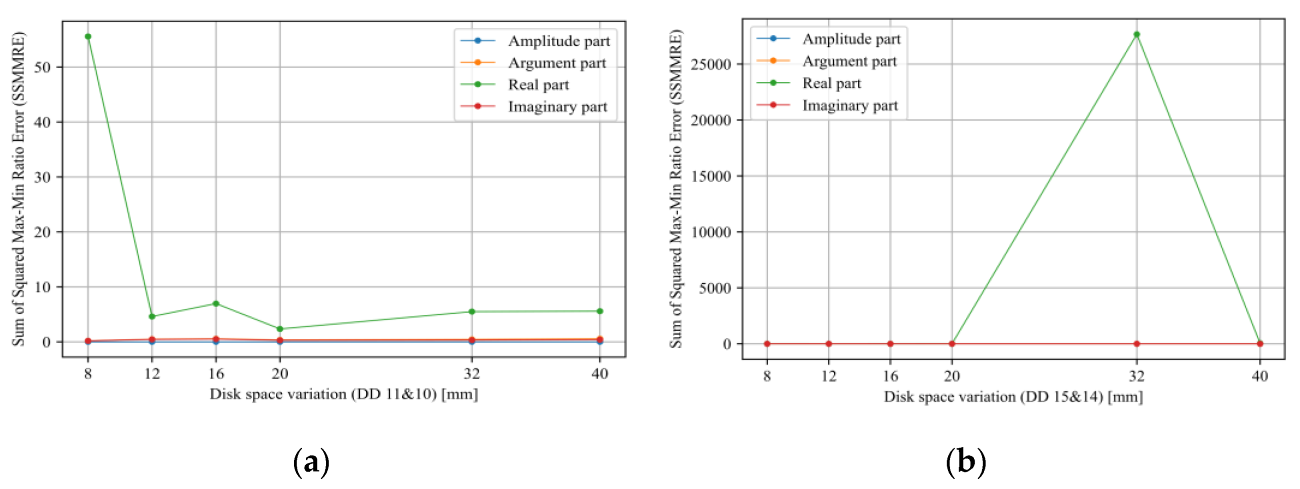
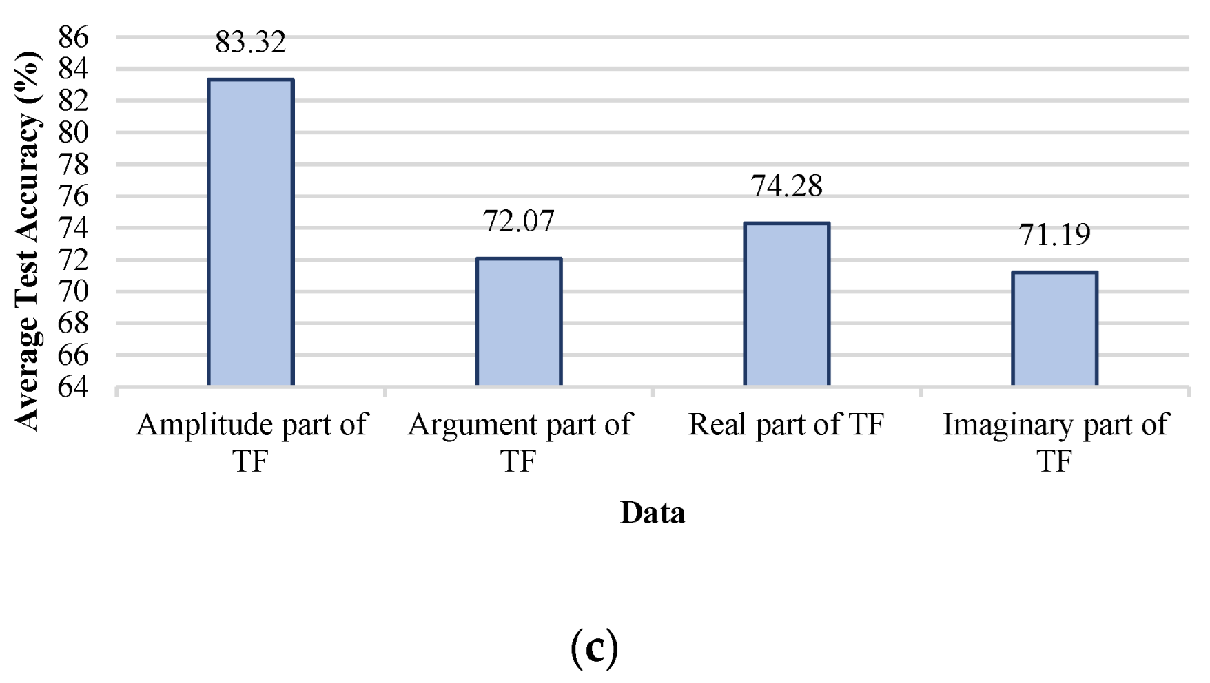
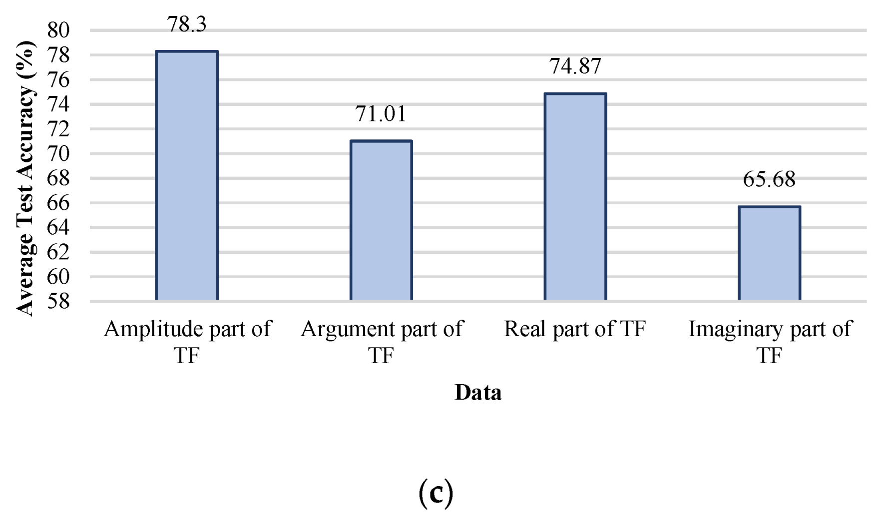
- Sensitivity analysis considering all TF parts (imaginary, real, magnitude, and phase) has been carried out.
2. Experimental Study and Data Preparation
2.1. Experimental Setup
2.2. Data Collection
3. Materials and Methods
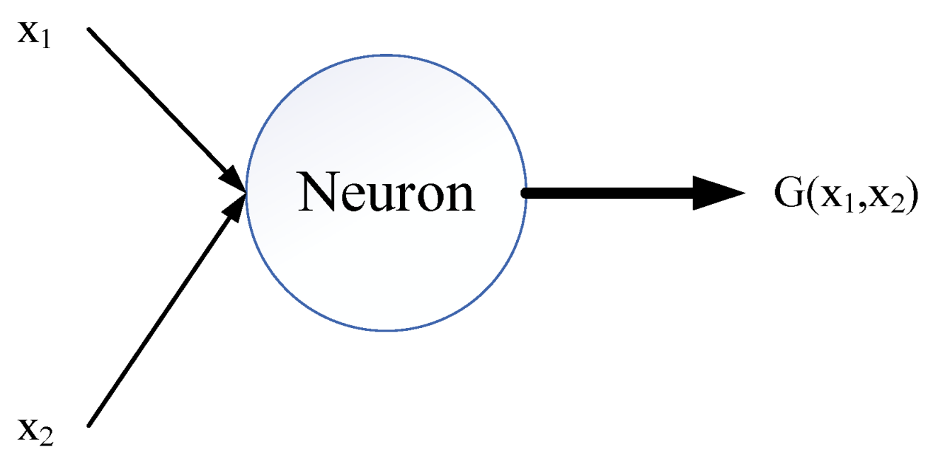
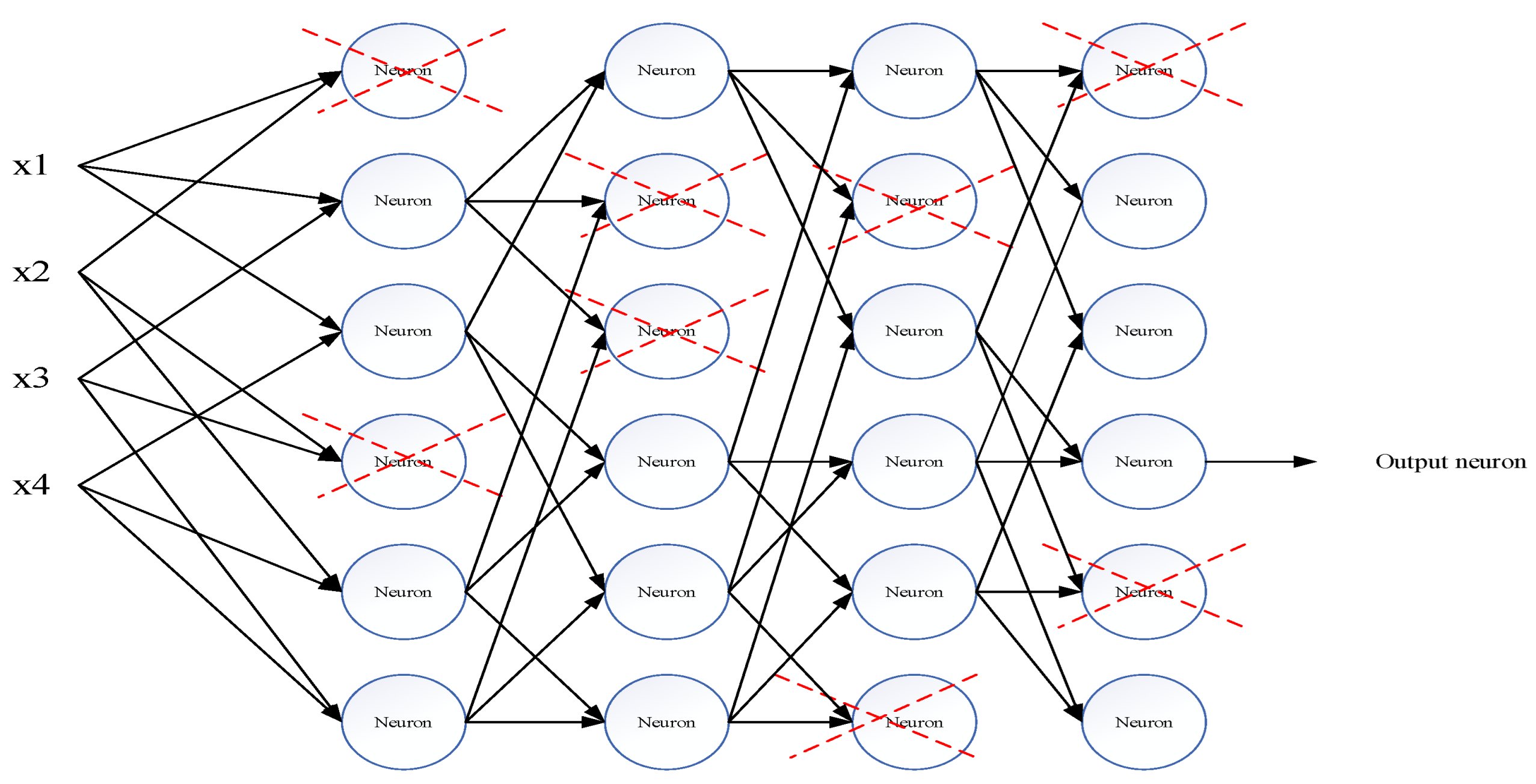
GMDH Artificial Neural Networks
4. Results
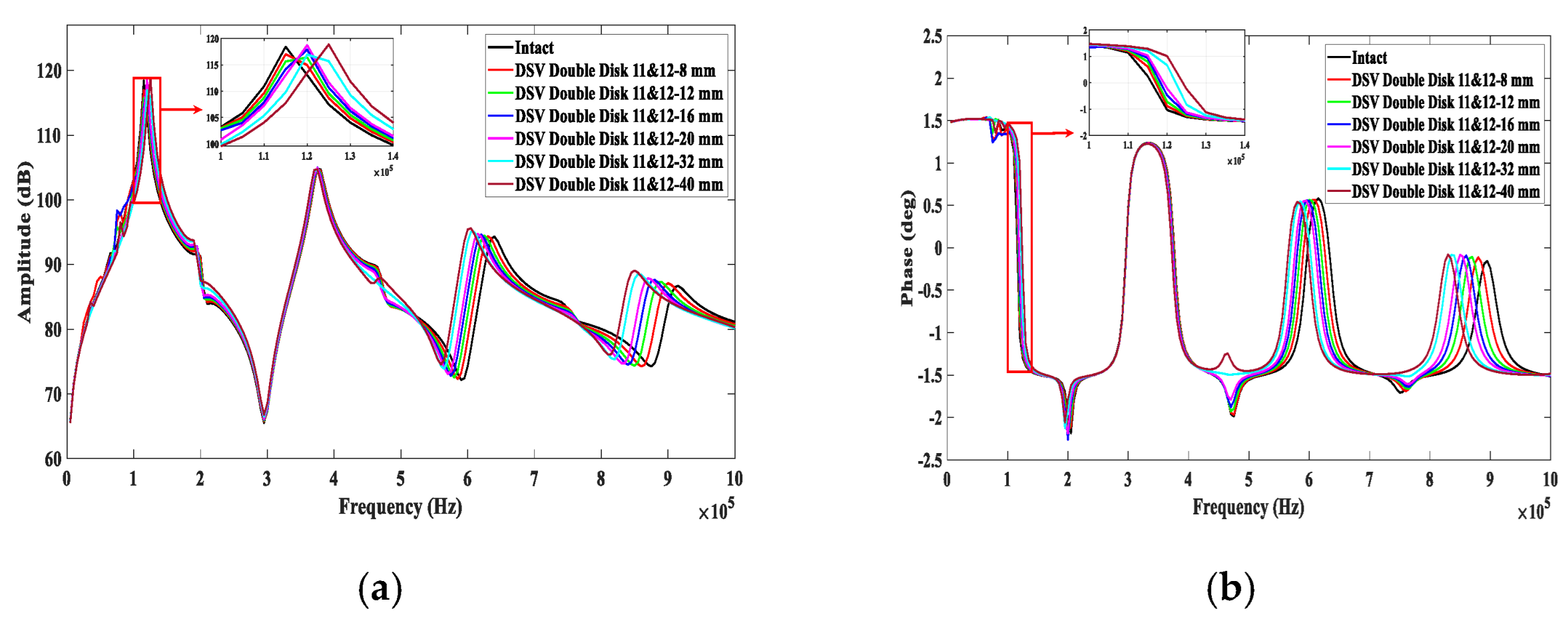
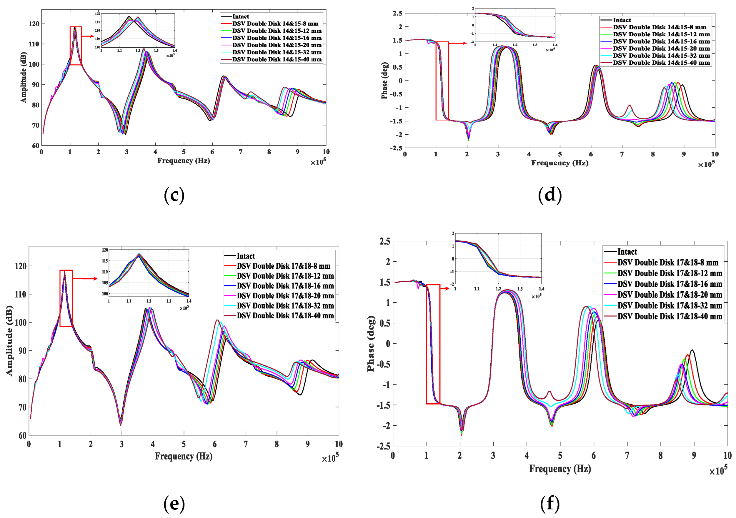
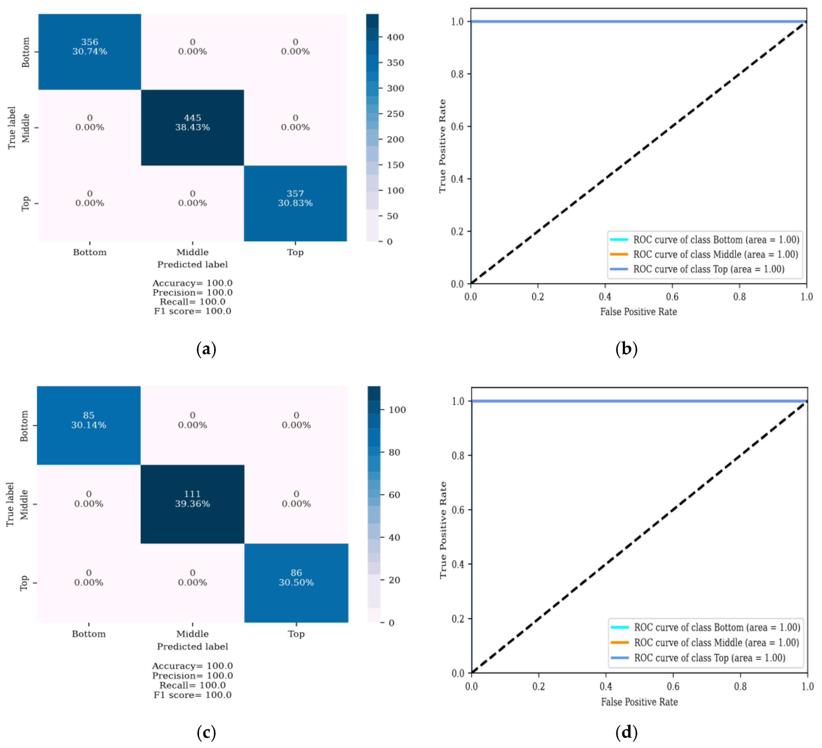
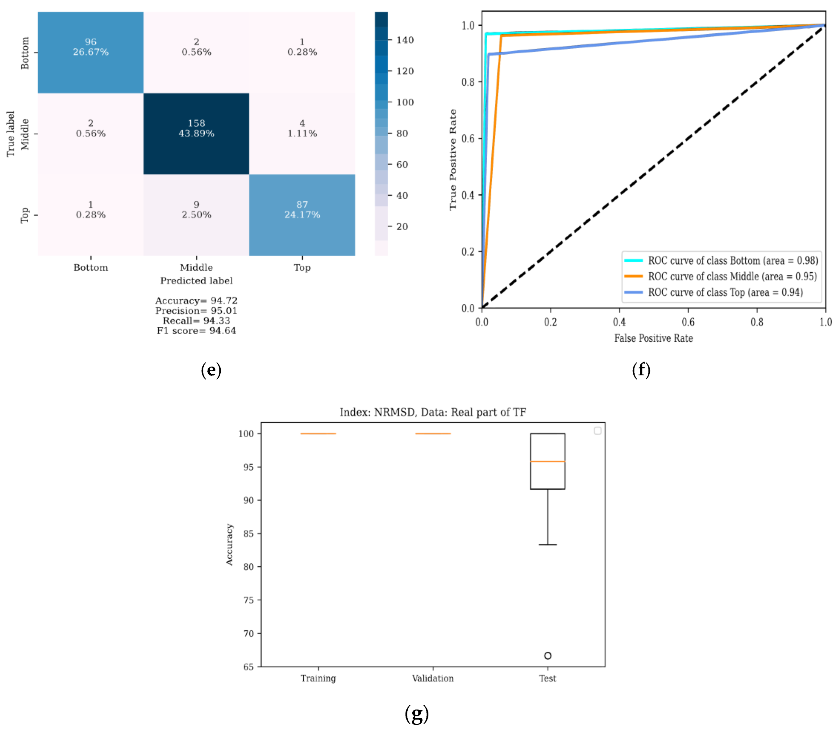
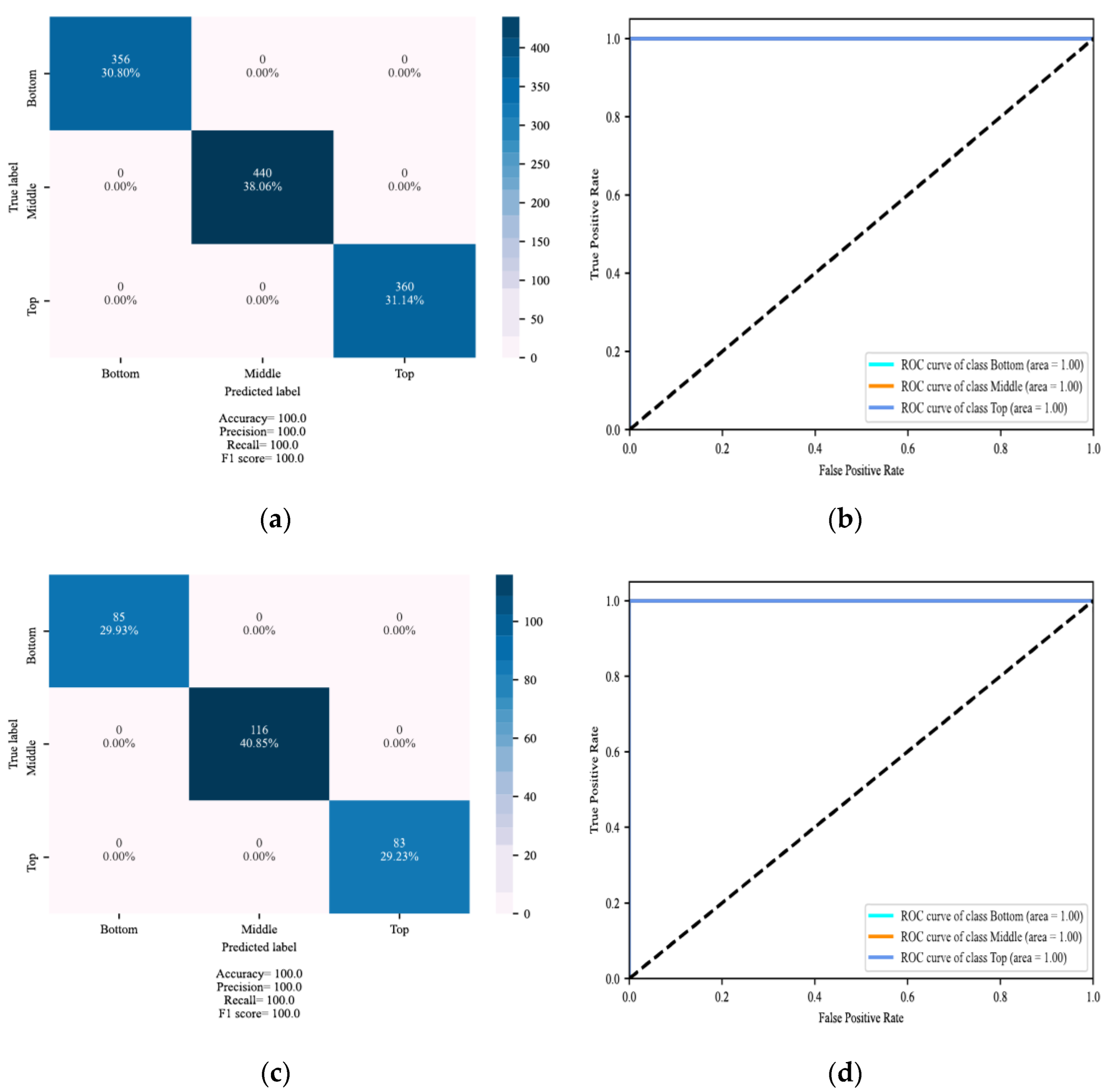
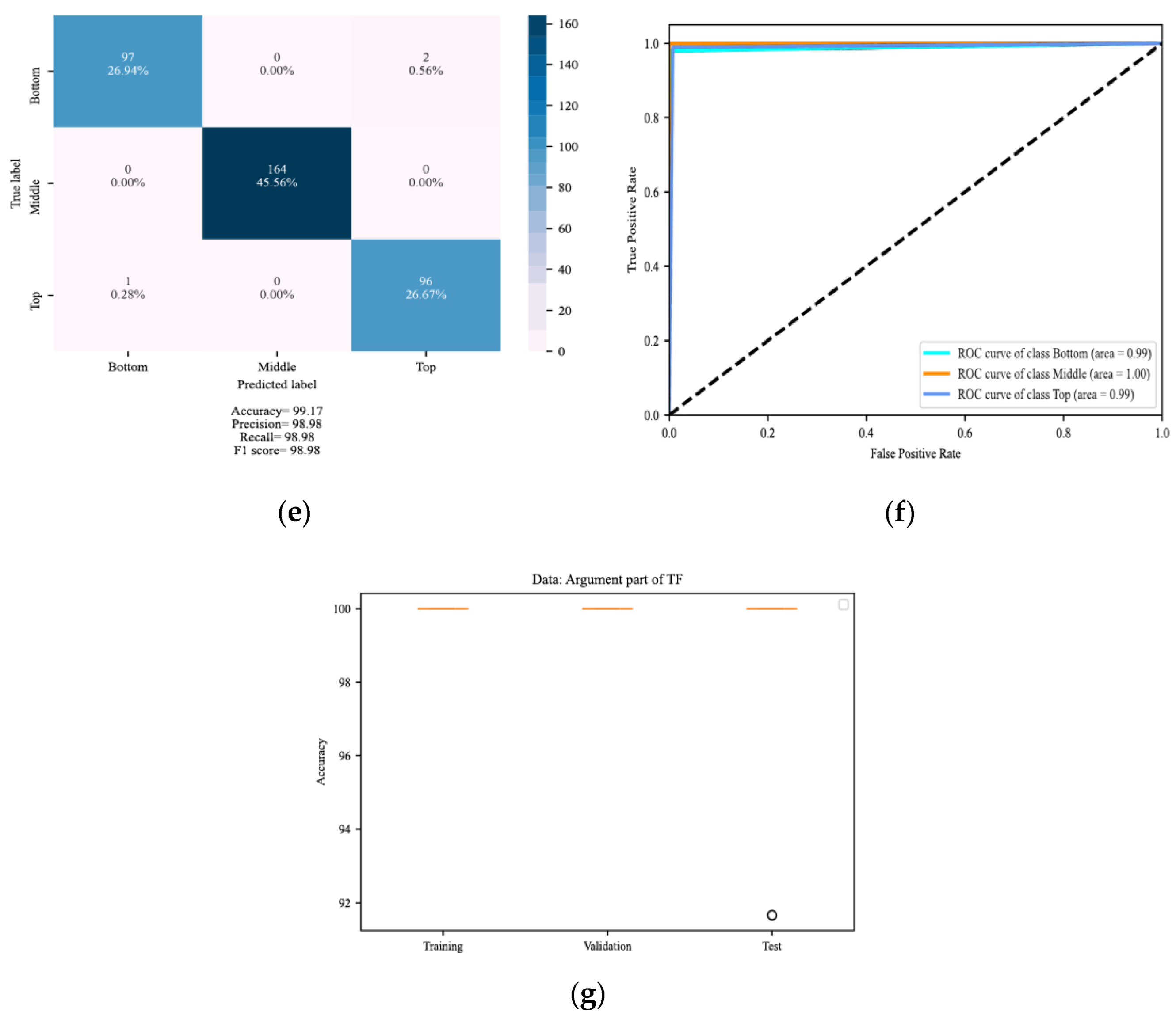
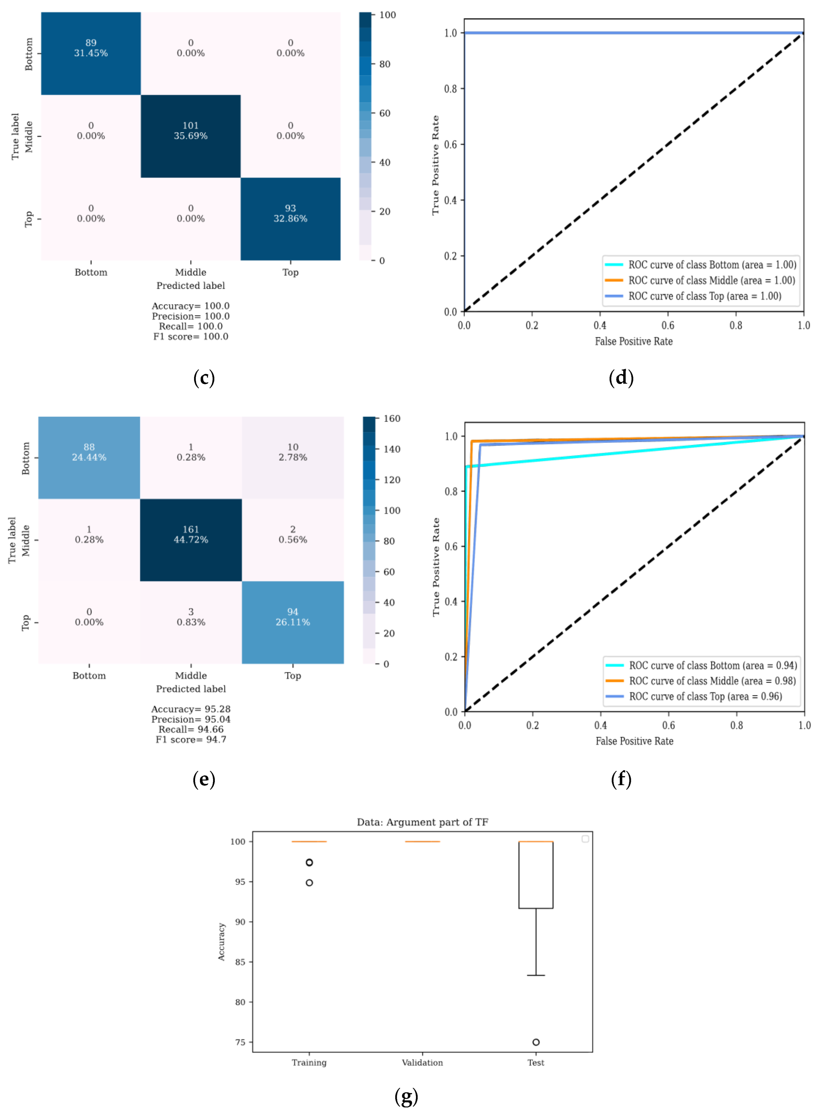
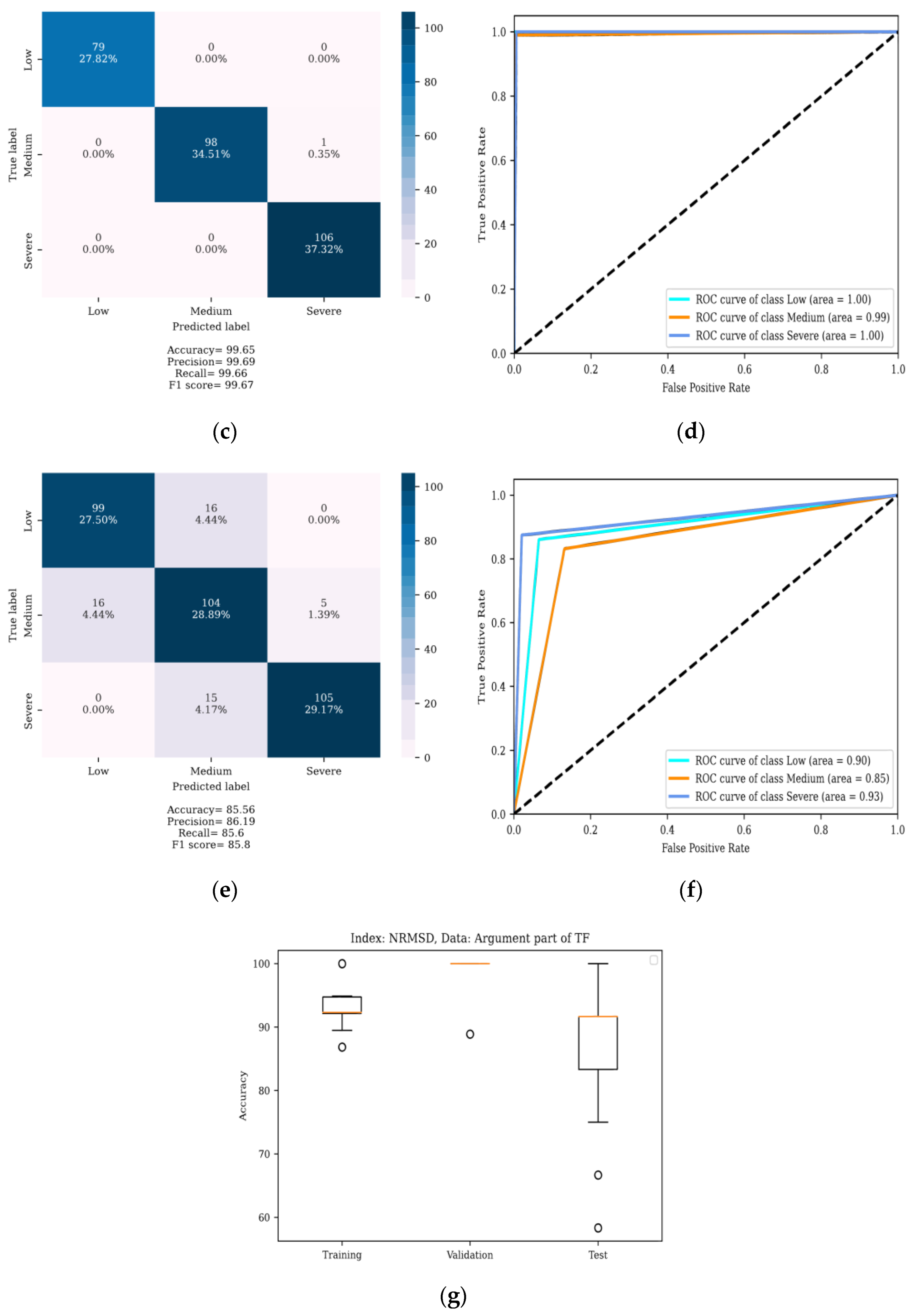
4.1. Localization of DSV Faults
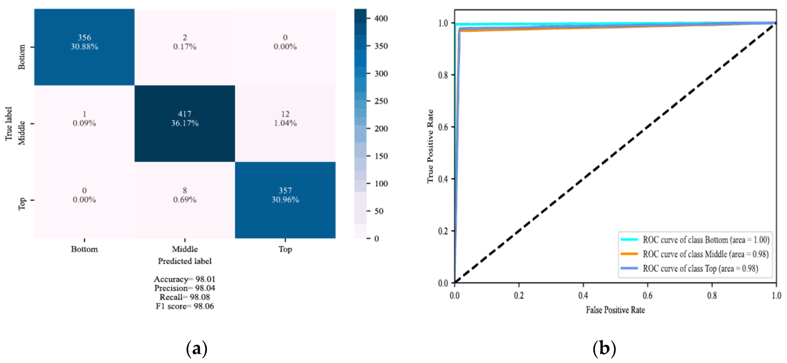
4.2. Determining the Severity of DSV Faults
5. Discussion
6. Conclusions
- ➢
- Using AI-based interpreters to identify simultaneous winding faults, such as detecting the simultaneous occurrence of RD and DSV faults with various intensities and locations;
- ➢
- Considering the effects of adjacent substation devices, such as Current Transformers (CTs), Potential Transformers (PTs), and other phases of a three-phase transformer on the phase in which the FRA test is performed for online monitoring.
Author Contributions
Funding
Data Availability Statement
Conflicts of Interest
Nomenclature
| SD | Spectrum Deviation |
| CCF | Cross Correlation Factor |
| CSD | Comparative Standard Deviation |
| LCC | Lin’s Concordance Coefficient |
| FP | Fitting Percentage |
| NRMSD | Normalized Root Mean Square Deviation |
| SE | Sum of Error |
| SSE | Sum of Squared Error |
| SSMMRE | Sum of Squared Max-Min Ratio Error |
| SSRE | Sum of Squared Ratio Error |
| DSV | Disk-Space Variation |
| DD | Double-Disk |
| GMDH | Group Method of Data Handling |
| NIns | Numerical Indicators |
| DPT | Distribution Power Transformer |
| FRA | Frequency Response Analysis |
| TF | Transfer Function |
| ANN | Artificial Neural Network |
| SVM | Support Vector Machine |
References
- Wei, X.; Gao, S.; Huang, T. Analysis of electrical network vulnerability using segmented cascading faults graph. Comput. Electr. Eng. 2019, 81, 106519. [Google Scholar] [CrossRef]
- Beura, C.P.; Beltle, M.; Wenger, P.; Tenbohlen, S. Experimental Analysis of Ultra-High-Frequency Signal Propagation Paths in Power Transformers. Energies 2022, 15, 2766. [Google Scholar] [CrossRef]
- Miyazaki, S. Detection of Winding Axial Displacement of a Real Transformer by Frequency Response Analysis without Fingerprint Data. Energies 2021, 15, 200. [Google Scholar] [CrossRef]
- Mohammadi, F.; Nazri, G.A.; Saif, M. A Fast Fault Detection and Identification Approach in Power Distribution Systems. In Proceedings of the IEEE 5th International Conference on Power Generation Systems and Renewable Energy Technologies (PGSRET), Istanbul, Turkey, 26–27 August 2019. [Google Scholar]
- Yang, Q.; Su, P.; Chen, Y. Comparison of Impulse Wave and Sweep Frequency Response Analysis Methods for Diagnosis of Transformer Winding Faults. Energies 2017, 10, 431. [Google Scholar] [CrossRef]
- Yoon, Y.; Son, Y.; Cho, J.; Jang, S.; Kim, Y.-G.; Choi, S. High-Frequency Modeling of a Three-Winding Power Transformer Using Sweep Frequency Response Analysis. Energies 2021, 14, 4009. [Google Scholar] [CrossRef]
- Tahir, M.; Tenbohlen, S. A Comprehensive Analysis of Windings Electrical and Mechanical Faults Using a High-Frequency Model. Energies 2019, 13, 105. [Google Scholar] [CrossRef] [Green Version]
- Bigdeli, M.; Abu-Siada, A. Clustering of transformer condition using frequency response analysis based on k-means and GOA. Electr. Power Syst. Res. 2021, 202, 107619. [Google Scholar] [CrossRef]
- Thango, B.A.; Nnachi, A.F.; Dlamini, G.A.; Bokoro, P.N. A Novel Approach to Assess Power Transformer Winding Conditions Using Regression Analysis and Frequency Response Measurements. Energies 2022, 15, 2335. [Google Scholar] [CrossRef]
- Banaszak, S.; Kornatowski, E.; Szoka, W. The Influence of the Window Width on FRA Assessment with Numerical Indices. Energies 2021, 14, 362. [Google Scholar] [CrossRef]
- Tahir, M.; Tenbholen, S.; Miyazaki, S. Analysis of Statistical Methods for Assessment of Power Transformer Frequency Response Measurements. IEEE Trans. Power Deliv. 2020, 36, 618–626. [Google Scholar] [CrossRef]
- Lu, S.; Gao, W.; Hong, C.; Sun, Y. A newly-designed fault diagnostic method for transformers via improved empirical wavelet transform and kernel extreme learning machine. Adv. Eng. Inform. 2021, 49, 101320. [Google Scholar] [CrossRef]
- Behkam, R.; Moradzadeh, A.; Karami, H.; Nadery, M.S.; Mohammadi-Ivatloo, B.; Gharehpetian, G.B.; Tenbohlen, S. Mechanical Fault Types Detection in Transformer Windings Using Interpretation of Frequency Responses via Multilayer Perceptron. J. Oper. Autom. Power Eng. 2022. [Google Scholar] [CrossRef]
- Zhao, Z.; Tang, C.; Zhou, Q.; Xu, L.; Gui, Y.; Yao, C. Identification of Power Transformer Winding Mechanical Fault Types Based on Online IFRA by Support Vector Machine. Energies 2017, 10, 2022. [Google Scholar] [CrossRef] [Green Version]
- Li, Z.; Zhang, Y.; Abu-Siada, A.; Chen, X.; Li, Z.; Xu, Y.; Zhang, L.; Tong, Y. Fault Diagnosis of Transformer Windings Based on Decision Tree and Fully Connected Neural Network. Energies 2021, 14, 1531. [Google Scholar] [CrossRef]
- Behkam, R.; Karami, H.; Naderi, M.S.; Gharehpetian, G.B. Condition Monitoring of Distribution Transformers Using Frequency Response Traces and Artificial Neural Network to Detect the Extent of Windings Axial Displacements. In Proceedings of the 26th International Electrical Power Distribution Conference (EPDC), Tehran, Iran, 11–12 May 2022; pp. 18–23. [Google Scholar] [CrossRef]
- Mohammadi, F.; Zheng, C. A precise SVM classification model for predictions with missing data. In Proceedings of the 4th National Conference on Applied Research in Electrical, Mechanical Computer and IT Engineering, Tehran, Iran, 4 October 2018. [Google Scholar]
- Mohammadi, F.; Zheng, C.; Su, R. Fault Diagnosis in Smart Grid Based on Data-Driven Computational Methods. In Proceedings of the 5th International Conference on Applied Research in Electrical, Mechanical, and Mechatronics Engineering, Tehran, Iran, 24 January 2019. [Google Scholar]
- Tahir, M.; Tenbohlen, S. Transformer Winding Condition Assessment Using Feedforward Artificial Neural Network and Frequency Response Measurements. Energies 2021, 14, 3227. [Google Scholar] [CrossRef]
- Moradzadeh, A.; Pourhossein, K.; Mohammadi-Ivatloo, B.; Mohammadi, F. Locating Inter-Turn Faults in Transformer Windings Using Isometric Feature Mapping of Frequency Response Traces. IEEE Trans. Ind. Inform. 2020, 17, 6962–6970. [Google Scholar] [CrossRef]
- MolaAbasi, H.; Khajeh, A.; Chenari, R.J. Use of GMDH-type neural network to model the mechanical behavior of a cement-treated sand. Neural Comput. Appl. 2021, 33, 15305–15318. [Google Scholar] [CrossRef]
- Cremer, J.L.; Strbac, G. A machine-learning based probabilistic perspective on dynamic security assessment. Int. J. Electr. Power Energy Syst. 2021, 128, 106571. [Google Scholar] [CrossRef]
- Mikheev, M.Y.; Gusynina, Y.S.; Shornikova, T.A. Building Neural Network for Pattern Recognition. In Proceedings of the 2020 International Russian Automation Conference (RusAutoCon 2020), Sochi, Russia, 6–12 September 2020; pp. 357–361. [Google Scholar] [CrossRef]
- Sesmero, M.P.; Alonso-Weber, J.M.; Sanchis, A. CCE: An ensemble architecture based on coupled ANN for solving multiclass problems. Inf. Fusion 2019, 58, 132–152. [Google Scholar] [CrossRef]
- Onwubolu, G. GMDH-Methodology and Implementation in MATLAB; Perlego Ltd.: London, UK, 2016. [Google Scholar]
- Tarimoradi, H.; Karami, H.; Gharehpetian, G.B.; Tenbohlen, S. Sensitivity analysis of different components of transfer function for detection and classification of type, location and extent of transformer faults. Measurement 2021, 187, 110292. [Google Scholar] [CrossRef]


| Index | Part of the TF |
|---|---|
| CCF | real |
| CSD | imaginary |
| FP | real |
| LCC | real |
| NRMSD | real |
| SD | cannot be defined |
| SE | phase |
| SSE | imaginary |
| SSMMRE | real |
| SSRE | real |
| Models | Determination of Location OR Severity | Average Time of Training Process Using NIns | Average Time of Training Process Using Raw FRA Data |
|---|---|---|---|
| GMDH | Location | 19.56 s | 50.62 s |
| Severity | 7.9 s | 29.62 s | |
| MLP | Location | 11.22 s | 28.89 s |
| Severity | 9.85 s | 11.02 s |
Publisher’s Note: MDPI stays neutral with regard to jurisdictional claims in published maps and institutional affiliations. |
© 2022 by the authors. Licensee MDPI, Basel, Switzerland. This article is an open access article distributed under the terms and conditions of the Creative Commons Attribution (CC BY) license (https://creativecommons.org/licenses/by/4.0/).
Share and Cite
Elahi, O.; Behkam, R.; Gharehpetian, G.B.; Mohammadi, F. Diagnosing Disk-Space Variation in Distribution Power Transformer Windings Using Group Method of Data Handling Artificial Neural Networks. Energies 2022, 15, 8885. https://doi.org/10.3390/en15238885
Elahi O, Behkam R, Gharehpetian GB, Mohammadi F. Diagnosing Disk-Space Variation in Distribution Power Transformer Windings Using Group Method of Data Handling Artificial Neural Networks. Energies. 2022; 15(23):8885. https://doi.org/10.3390/en15238885
Chicago/Turabian StyleElahi, Omid, Reza Behkam, Gevork B. Gharehpetian, and Fazel Mohammadi. 2022. "Diagnosing Disk-Space Variation in Distribution Power Transformer Windings Using Group Method of Data Handling Artificial Neural Networks" Energies 15, no. 23: 8885. https://doi.org/10.3390/en15238885