A Comprehensive Review of Photovoltaic Modules Models and Algorithms Used in Parameter Extraction

Abstract

Currently, solar energy is one of the leading renewable energy sources that help support energy transition into decarbonized energy systems for a safer future. This work provides a comprehensive review of mathematical modeling used to simulate the performance of photovoltaic (PV) modules. The meteorological parameters that influence the performance of PV modules are also presented. Various deterministic and probabilistic mathematical modeling methodologies have been investigated. Moreover, the metaheuristic methods used in the parameter extraction of diode models of the PV equivalent circuits are addressed in this article to encourage the adoption of algorithms that can predict the parameters with the highest precision possible. With the significant increase in the computational power of workstations and personal computers, soft computing algorithms are expected to attract more attention and dominate other algorithms. The different error expressions used in formulating objective functions that are employed in extracting the parameters of PV models are comprehensively expressed. Finally, this work aims to develop a comprehensive layout for the previous, current, and possible future areas of PV module modeling.

1. Introduction

The world suffered in the past years from two significant crises. The first is COVID-19 [1], which interrupted the energy supply chain and its management. The second is the Ukraine-Russia war [2], which affected energy policy in all its aspects globally and pushed many countries to adopt a greener energy policy. In light of the ongoing energy crises, the global tendency is to find an alternative. The alternative should be environmentally friendly, have green resources, and help to decarbonize electrical generation. Hence, the importance of all renewable energy resources arises. Renewable resources are wind, solar, tides, waves, etc. Some of these resources are mature with ongoing research and development, such as wind and solar power (concentrated solar power and photovoltaics). At the same time, other renewable energy resources are still under development and feasibility evaluation, such as ocean power (tides and waves). There is a global transition and concern about photovoltaic (PV) systems. Photovoltaics offer an appealing alternative: zero emissions, noise-free, modular, and low maintenance [3,4,5].

Efficient models are crucially needed to harness the advantages mentioned above. The models contribute to various general fields related to PV systems, such as design, simulation, control, planning, performance evaluation [6], and siting and sizing [7,8]. Therefore, developing and updating various models are of vital importance.

This review article presents the different models of PV module models: the single “one” diode model (SDM), the double “two” diode model (DDM), and the triple/three diode model (TDM). The models relate PV module I-V mathematical modeling to datasheet values. They also consider the effect of meteorological parameters on PV module parameters. This paper aims to provide the mathematical equations that describe various PV models, regardless of the technology used.

For PV parameter extraction, the paper presents 14 analytical models for SDM, 6 analytical models for DDM, and 2 analytical models for TDM. Concerning the soft computing algorithms, more than 35 different algorithms were presented. Some equations were repeated intentionally to make a specific PV model complete. This decreases the reader’s distraction with equation references from other models.

The review article is organized as follows: Section 2 presents the configurations of SDM, DDM, and TDM; Section 3 presents an overview of PV technologies; Section 4 presents a list of various error measurement models; Section 5 presents a comprehensive list of all the algorithms used in extracting the parameters of different PV module models; and Section 6 presents the conclusions drawn from this work.

2. Mathematical Modeling of Single, Double, and Triple Diode Equivalent Circuits

This section presents a comprehensive review of the published work concerning analytical trials conducted to estimate the three most well-known models for PV modules. Those models are:

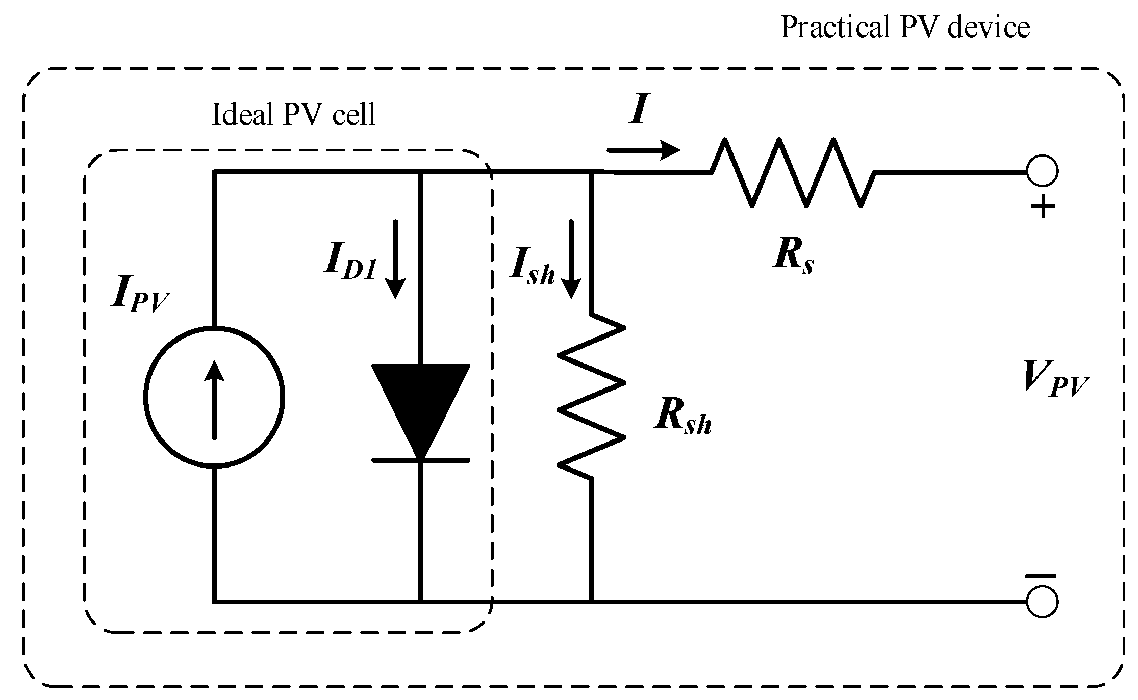
• Single Diode Model (SDM);
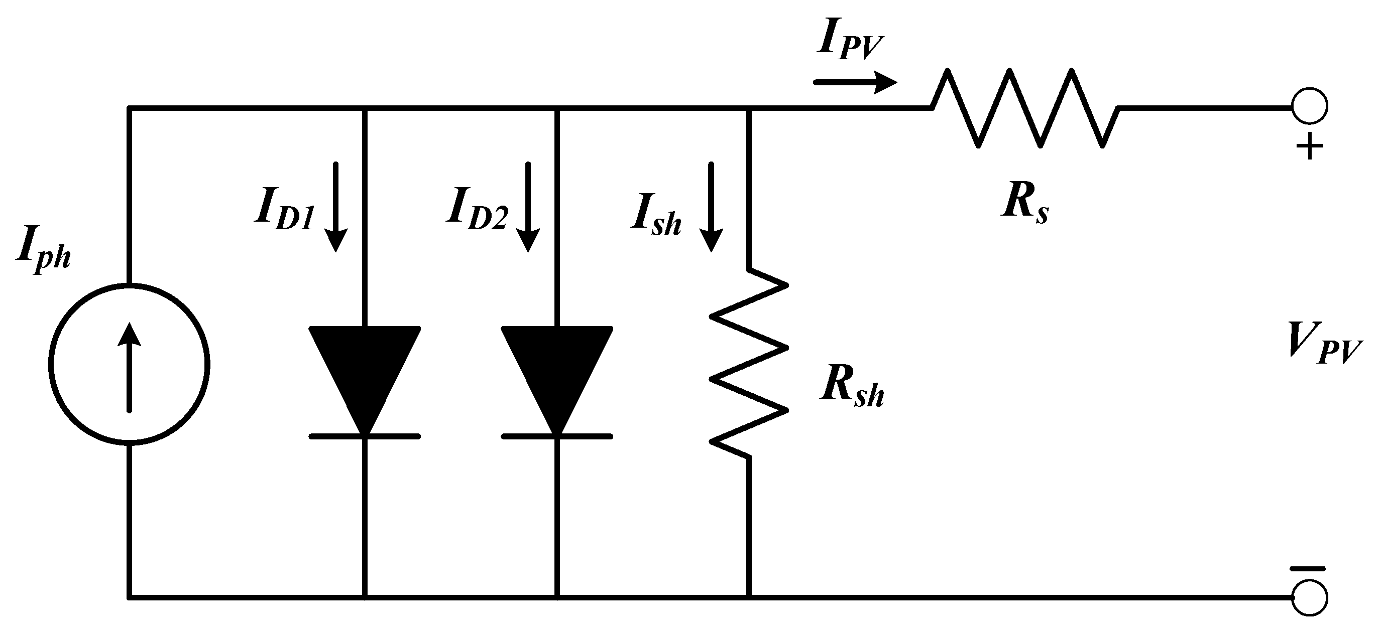
• Double Diode Model (DDM);
• Triple Diode Model (TDM).

Other models can represent PV modules as well, but they are out of this article’s scope.

2.1. Single Diode Model (SDM): Parameters Estimation

This is the most basic and straightforward circuit representation for the PV module. This model contains a single diode, shunt and series resistance, and irradiance source.

The values provided by the PV manufacturer are the open circuit voltage ($V_{OC}$), short circuit current ($I_{SC}$), maximum power point current ($I_{MPP}$) and voltage ($V_{MPP}$), and maximum power ($P_{MPP}$). Some manufacturers’ datasheets offer the temperature dependence coefficient for the short circuit current ($K_I$) and the open circuit voltage ($K_V$). However, the PV model has other values that specify the module’s performance. The PV model values are photocurrent/light current ($I_{PV}$), reverse saturation current ($I_O$), ideality constant of the diode ($a$), and the resistances, shunt ($R_{SH}$), series ($R_S$). Therefore, the PV model parameters need methodologies calculated from the datasheet values. The methods can be analytical/deterministic or metaheuristic/probabilistic [9].

2.1.1. Parameter Estimation of SDM—Analytical Method #01

Any PV module contains many solar cells. Thus, to obtain the I-V characteristics of a PV module, the I-V characteristics of the ideal solar cell shall be used. The exemplary solar cell has the following mathematical formula:

$$I=I_{PV}-I_{D1}$$

(1)

$$I_{D1}=I_{01}\left[exp\left(\frac{q{V}_{PV}}{a_{1}KT}\right)-1\right]$$

(2)

Substituting (2) into (1), then

$$I=I_{PV.cell}-I_{01}\left[exp\left(\frac{q{V}_{PV}}{a_{1}KT}\right)-1\right]$$

(3)

Therefore, Equation (3) becomes:

$$I=I_{PV}-I_{01}\left[exp\left(\frac{q\left(V_{PV}+R_{s}I\right)}{N_{CS}{a}_{1}KT}\right)-1\right]-\frac{V_{PV}+R_{s}I}{R_{sh}}$$

(4)

But the term $V_t=\frac{N_{CS}KT}{q}$, thus introducing the last term to (4) leads to:

$$I=I_{PV}-I_{01}\left[exp\left(\frac{V_{PV}+R_{s}I}{a_1{V}_t}\right)-1\right]-\frac{V_{PV}+R_{s}I}{R_{sh}}$$

(5)

To model the PV module (single diode one), additional parameters shall be added, as illustrated in Figure 1.

Where

$I_{PV.cell}$	Total current generated from PV cell
$I_{PV}$	Light current, i.e., generated due to solar irradiance
$I_{D1}$	Shockley diode current (single diode)
$I_{01}$	Reverse saturation/leakage current of diode
$q$	Electron charge ($1.60217646\times {10}^{-19} C$)
$V_{PV}$	Voltage across the device
$a_1$	Ideality constant of the diode (single diode)
$K$	Boltzmann constant ($1.3806503\times {10}^{-23} J/K$)
$T$	p-n junction temperature (Kelvin)
$R_s$	Equivalent series resistance
$R_{sh}$	Equivalent shunt resistance
$V_t$	Thermal voltage of the PV module
$N_{CS}$	Number of series connected cells that form the PV module (provided by the manufacturer)

The accuracy of the SDM is not the best, and it can be further enhanced. The enhancement increases by adding extra diodes to the previously illustrated model, which is then named the double diode model (DDM) and the triple diode model (TDM).

Equation (5) has five unknown parameters, which are ($I_{PV}$, $I_{01}$, $a_1$, $R_s$, and $R_{sh}$). There are several methods to find the values of those parameters. The methods are categorized into analytical and metaheuristic methods. The analytical methods use equations to evaluate the parameters. For the $I_{PV}$, it has the following formula:

$$I_{PV}=\left(I_{PV.n}+K_I\left(T-T_n\right)\right)\frac{G}{G_n}$$

(6)

where

• $I_{PV.n}$—Light current (A) at nominal conditions (25 °C and 1000 W/m²)
• $K_I$—Temperature coefficient for short circuit current (A/K)
• $T$—Actual temperature (K)
• $T_n$—Nominal temperature (K)
• $G$—Solar insolation at PV panel surface (W/m²)
• $G_n$—Solar insolation at nominal conditions (W/m²)

Afterward, the saturation current $I_{01}$ has the following equation:

$$I_{01}=I_{01.n}{\left(\frac{T_n}{T}\right)}^{3}exp\left(\frac{q{E}_g}{a_{1}k}\left(\frac{1}{T_n}-\frac{1}{T}\right)\right)$$

(7)

where E_g denotes the semiconductor bandgap energy.

Finally, $I_{01.n}$ can be calculated as follows:

$$I_{01.n}=\frac{I_{SC.n}}{exp\left(\frac{V_{OC.n}}{a_1{V}_{t.n}}\right)-1}$$

(8)

where

• $I_{SC.n}$—Short circuit current at the nominal conditions
• $V_{OC.n}$—Open circuit voltage at the nominal conditions.

The authors in [10,11,12] suggested replacing Equation (7) with another new equation; thus, the parameter estimation methodology is improved. The equation is given as follows:

$$I_{01}=\frac{I_{SC.n}+K_I\left(T-T_n\right)}{exp\left(\frac{V_{OC.n}+K_V\left(T-T_n\right)}{a_1{V}_{t,n}}\right)-1}$$

(9)

Equation (9) improves Equation (8) by utilizing both current and voltage temperature coefficients. Thus, the error of the previous model is eliminated, where $K_V$—Temperature coefficient for open circuit voltage (A/K).

The diode ideality factor value varies as follows: $1\le a_1\le 1.5$. Any initial value can be selected as a start and then finetuned later. The variation of $a_1$ affects the accuracy of the methodology. The values of $R_s \& R_{sh}$ are still undetermined. To find both without neglecting any of them, the authors in [10,11,12] suggested that there is a single pair of $R_s \& R_{sh}$ that will make both I-V & P-V curves fit the manufacturer’s datasheet. This pair can be found by assuming the maximum power calculated using Equation (5) ($P_{max.m}$) equals to the nominal power of the PV array ($P_{max.e}$). The latter value can be found in the manufacturer’s data sheet. The derivation for the required equation, based on Equation (5), is given as follows:

$$P_{max.m}=V_{mp}\left\{I_{PV}-I_{01}\left[exp\left(\frac{q\left(V_{mp}+R_s{I}_{mp}\right)}{a_1{V}_t}\right)-1\right]-\frac{V_{mp}+R_s{I}_{mp}}{R_{sh}}\right\}=P_{max.e}$$

(10)

Ordering the terms in Equation (10) to find an equation for $R_P$, will be expressed as follows:

$$\begin{array}{c}{V}_{mp}{I}_{PV}-V_{mp}{I}_{01}\left[exp\left(\frac{q\left(V_{mp}+R_s{I}_{mp}\right)}{a_1{V}_t}\right)\right]+V_{mp}{I}_{01}-V_{mp}\left(\frac{V_{mp}+R_s{I}_{mp}}{R_{sh}}\right)=P_{max.e}\\ V_{mp}{I}_{PV}-V_{mp}{I}_{01}\left[exp\left(\frac{q\left(V_{mp}+R_s{I}_{mp}\right)}{a_1{V}_t}\right)\right]+V_{mp}{I}_{01}-P_{max,e}=V_{mp}\left(\frac{V_{mp}+R_s{I}_{mp}}{R_{sh}}\right)\\ R_{sh}=\frac{V_{mp}\left(V_{mp}+R_s{I}_{mp}\right)}{\left\{V_{mp}{I}_{PV}-V_{mp}{I}_{01}\left[exp\left(\frac{q\left(V_{mp}+R_s{I}_{mp}\right)}{a_1{V}_t}\right)\right]+V_{mp}{I}_{01}-P_{max.e}\right\}}\end{array}$$

(11)

The light current $I_{PV}$ is still undetermined and can also be found using numerical methods via Equation (5). The authors suggested using the following equation to get the value for $I_{PV}$. The equation is given as follows:

$$I_{PV.n}=\frac{R_{sh}+R_s}{R_{sh}}{I}_{SC.n}$$

(12)

The initial value for $R_{sh.inital}$ was suggested to be as follows:

$$R_{sh.inital}=\frac{V_{mp}}{I_{SC.n}-I_{mp}}-\frac{V_{OC.n}-V_{mp}}{I_{mp}}$$

(13)

2.1.2. Parameter Estimation of SDM—Analytical Method #02

The authors in [13] used the following set of equations for modeling and parameter estimation of SDM. The model starting equations are given as follows:

$$I=I_{PV}-I_{01}\left[exp\left(\frac{V_{PV}+R_{s}I}{a_1{V}_t}\right)-1\right]-\frac{V_{PV}+R_{s}I}{R_{sh}}$$

(14)

$$I_{SC}=I_{SC.n}\frac{G}{G_n}+K_I\left(T-T_n\right)$$

(15)

$$V_{OC}=V_{OC.n}+K_V\left(T-T_n\right)+a_1{V}_{t}ln\left(\frac{G}{G_n}\right)$$

(16)

The model has the following initial conditions: ($0, V_{OC.n})$; ($I_{SC.n}, 0$); ($I_{MPP.n}, V_{MPP.n}$); ($I_{MPP.n}, V_{MPP.n}$). Then to estimate the series and shunt resistances, the following equations are used:

$$R_{S,0}=-\frac{d{V}_{OC}}{dI}$$

(17)

$$R_{SH,0}=-\frac{dV}{d{I}_{SC}}$$

(18)

Finally, the following equations can be used to estimate the model parameters:

$$I_{PV}=I_{SC}\left(1+\frac{R_s}{R_{sh}}\right)I_{01}\left[exp\left(\frac{I_{SC}{R}_s}{a_1{V}_t}\right)-1\right]$$

(19)

$$I_{01}=\left(I_{SC}-\frac{V_{OC}}{R_{sh}}\right)\left[exp\left(\frac{V_{OC}}{a_1{V}_t}\right)\right]$$

(20)

$$R_S=R_{S,0}-\frac{a_1{V}_t}{I_{01}}\left[exp\left(-\frac{V_{OC}}{a_1{V}_t}\right)\right]$$

(21)

$$R_{SH}=R_{SH,0}$$

(22)

$$a_1=\frac{V_{MPP}+I_{MPP}{R}_{S,0}-V_{OC}}{V_t\left\{ln\left(I_{SC}-\frac{ V_{MPP}}{R_{SH}}-I_{MPP}\right)-ln\left(I_{SC}-\frac{ V_{OC}}{R_{SH}}\right)+\left(\frac{I_{MPP}}{I_{SC}-\frac{ V_{OC}}{R_{SH}}}\right)\right\}}$$

(23)

The details for finding the derivatives ($\frac{d{V}_{OC}}{dI}$, $\frac{dV}{d{I}_{SC}}$) can be found in [14]. The values of $I_{SC}$ & $V_{OC}$ are obtained using Equations (15) and (16), respectively, then the rest of the values ($a_1$, $R_S$, $I_{01}$, and $I_{PV}$) using the previously mentioned equations.

2.1.3. Parameter Estimation of SDM—Analytical Method #03

The authors in [15] used the following set of equations for PV of type SDM, but the estimation of ($I_{01}$) was based on the international standard coded by IEC891:

$$I=I_{PV}-I_{01}\left[exp\left(\frac{V_{PV}+R_{s}I}{a_1{V}_t}\right)-1\right]-\frac{V_{PV}+R_{s}I}{R_{sh}}$$

(24)

$$I_{01}\left(T\right)=D{T}^3\left[exp\left(\frac{q{E}_{g.n}}{a_{1}KT}\right)\right]$$

(25)

Using the same initial conditions mentioned in analytical method #2, the series and shunt resistances are initialized as follows:

$$R_{S.0}=-\frac{d{V}_{OC}}{dI}$$

(26)

$$R_{SH.0}=-\frac{dV}{d{I}_{SC}}$$

(27)

The model continues as follows for estimating the rest of the model parameters:

$$I_{PV}=I_{01}\left[exp\left(\frac{V_{OC}}{a_1{V}_t}\right)-1\right]+\frac{V_{OC}}{R_{SH}}$$

(28)

$$I_{01}=\frac{I_{SC}\left(\frac{R_S}{R_{SH}}\right)-\frac{V_{OC}}{R_{SH}}}{exp\left(\frac{V_{OC}}{a_1{V}_t}\right)}$$

(29)

$$R_S=\frac{R_{S.0}\left(\frac{V_{OC}}{a_1{V}_t}-1\right)+R_{SH.0}\left(1-\frac{I_{SC}{R}_{S.0}}{a_1{V}_t}\right)}{\frac{V_{OC}-I_{SC}{R}_{SH.0}}{a_1{V}_t}}$$

(30)

$$R_{SH}=R_{SH.0}-R_S$$

(31)

$$a_1=\frac{V_{MPP}+I_{MPP}{R}_S-V_{OC}}{V_t\times ln\left(\frac{ I_{SC}-I_{MPP}\left(1+\frac{R_S}{R_{SH}}\right)-\frac{V_{MPP}}{R_{SH}}}{ I_{SC}\left(1+\frac{R_S}{R_{SH}}\right)-\frac{V_{OC}}{R_{SH}}}\right)}$$

(32)

The model starts with the initial value for $R_S$, then the value of $R_{SH}$ and $a_1$ are obtained. In turn, the value of $R_S$ is obtained. The new value of $R_S$ is then compared with the previous ones. Iterations are done to reach a value of $R_S$ that is equal to the previous one. The values of $R_{SH}$, $I_{PV}$, and $I_{01}$, are then computed, where

• $R_{S.0}$—Reciprocal of slope at open circuit point
• $R_{SH.0}$—Reciprocal of slope at short circuit point

2.1.4. Parameter Estimation of SDM—Analytical Method #04

The authors in [16] used concepts developed at Sandia laboratories for a decade. The model uses the data provided by the PV manufacturer, along with other calculated parameters known as “empirical parameters”. Those parameters are addressed hereunder. This model can be used in various applications, including sizing and monitoring the actual output versus the estimated output. In addition, it can be adapted to any PV technology (thin film, polycrystalline, mono-crystalline, etc.). The model starts as follows:

$$I=I_{PV}-I_{01}\left[exp\left(\frac{V_{PV}+R_{s}I}{A_m}\right)-1\right]-\frac{V_{PV}+R_{s}I}{R_{sh}}$$

(33)

$$A_m=\frac{a_{1}kT}{q}$$

(34)

$$I_{PV}=I_{SC.n}\left(\frac{G}{G_n}\times \frac{M}{M_n}\right)\left(1+K_I\left(T-T_n\right)\right)$$

(35)

$$I_{01}=I_{01.n}{\left(\frac{T}{T_n}\right)}^3\left[exp\left(\frac{1}{K}\left(\frac{q{E}_{g.n}}{T_n}-\frac{q{E}_g}{T}\right)\right)\right]$$

(36)

$$R_{SH}=R_{SH.n}\left(\frac{G}{G_n}\right)$$

(37)

$$A_m=A_{m.n}\left(\frac{T}{T_n}\right)$$

(38)

$$K_V=\frac{V_{OC.n}-V_{OC}}{T_n-T}$$

(39)

where

• $a_{1.n}$—Ideality constant (at nominal conditions)
• $A_m$—Air mass
• $A_{m.n}$—Air mass (at nominal conditions)
• $E_{g.n}$—Energy bandgap at reference temperature (=1.12 eV for silicon)
• $I_{01.n}$—Reverse saturation/leakage current of the diode (at nominal conditions)
• $M$—Air mass modifier
• $M_n$—Air mass at standard rating conditions
• $R_{S.n}$—Series resistance (at nominal conditions)
• $R_{SH.n}$—Shunt resistance (at nominal conditions)

The model has the following initial conditions: ($0,V_{OC.n}$); ($I_{SC.n},0$); ($I_{MPP.n},V_{MPP.n}$); ($\raisebox{1ex}{$dP$}\!\left/ \!\raisebox{-1ex}{$d{V}_{MPP}$}\right.=0$). To solve (39), the following equations shall be solved using Engineering Equation Solver (EES) along with Equation (36) [17]:

$$\frac{a_1}{a_{1.n}}=\frac{T}{T_n}$$

(40)

$$\frac{E_g}{E_{g.n}}=1-0.0002677\left(T-T_n\right)$$

(41)

$$I_{PV}=\frac{G}{G_n}\frac{M}{M_n}\left(I_{PV.n}+K_I\left(T-T_n\right)\right)$$

(42)

The authors in [18] modified the model to be suitable for an array of PV panels connected in series and parallel. In addition, they introduced the use of MATLAB instead of EES to evaluate the Equations (36) and (40)–(42).

Another attempt was made in [19,20] to reduce the equations’ five parameter equations into only two equations in terms of $a_{1.n}$ and $R_{Sn}$. This reduction in the number of variables guarantees that the nonlinear solver will converge to a solution at its first launch.

2.1.5. Parameter Estimation of SDM—Analytical Method #05

The authors in [21] introduced a new model for PV modules, as follows:

$$\begin{array}{c}I\left({\alpha }_G.T\right)={\alpha }_G{I}_{PV}\left(T\right)-I_{01}\left({\alpha }_G.T\right)\left[exp\left(\frac{{\alpha }_G\left[V_{PV}+K_{TH}I\left(T-T_n\right)\right]+I{R}_S}{{\alpha }_G{a}_{1}T}\right)-1\right]\\ -\frac{{\alpha }_G\left[V_{PV}+K_{TH}I\left(T-T_n\right)\right]+I{R}_S}{R_{SH}}\end{array}$$

(43)

$${\alpha }_G=\left(\frac{G}{G_n}\right)$$

(44)

$$K_{TH}=\frac{V_{MPP.0}-V_{MPP}^{*}}{I_{MPP}^{*}\left(T^{*}-T_n\right)}$$

(45)

$$I_{PV}=I_{PV.n}+K_I\left(T-T_n\right)$$

(46)

$$V_{OC}\left({\alpha }_G.T\right)=V_{OC.n}\left({\alpha }_G\right)+K_V\left(T-T_n\right)$$

(47)

$$R_{SH}\left({\alpha }_G\right)=\frac{R_S}{{\alpha }_G}$$

(48)

$$R_{SH}\left({\alpha }_G\right)=\frac{R_{SH}}{{\alpha }_G}$$

(49)

$$I_{01}\left({\alpha }_G.T\right)=exp\left\{\left(\frac{{\alpha }_G-0.2}{1-0.2}\right)ln\left(\frac{I_{01}\left(1.T\right)}{I_{01}\left(0.2.T\right)}\right)+ln\left(I_{01}\left(0.2.T\right)\right)\right\}$$

(50)

To calculate the values of ($I_{01}\left(1.T\right)$)and ($I_{01}\left(0.2.T\right)$), the authors in [21] used the following equation:

$$I_{01}\left({\alpha }_G.T\right)={\alpha }_G\left(\frac{I_{PV}\left(T\right)-\frac{V_{OC}\left({\alpha }_G.T\right)}{R_{SH}}}{exp\left(\frac{V_{OC}\left({\alpha }_G.T\right)}{a_{1}T}\right)-1}\right)$$

(51)

where

• ${\alpha }_G$—The ratio between current irradiance and irradiance at standard rating conditions
• $K_{TH}$—Thermal correction factor ($\mathrm{\Omega }/$°C)
• $V_{MPP}^{*}$—The voltage at maximum power point (at standard irradiance = 1000 W/m²)
• $I_{MPP}^{*}$—Current at maximum power point (at standard irradiance = 1000 W/m²)
• $T^{*}$—PV cell temperature (the value lies between the minimum and maximum values provided in the manufacturer’s datasheet)

The model has the following initial conditions: ($0, V_{OC.n}$); ($I_{SC.n}, 0$); ($I_{MPP.n}, V_{MPP.n}$); ($R_{S.0}=-\raisebox{1ex}{$d{V}_{OC}$}\!\left/ \!\raisebox{-1ex}{$dI$}\right.$) and ($R_{SH.0}=-\raisebox{1ex}{$dV$}\!\left/ \!\raisebox{-1ex}{$d{I}_{SC}$}\right.$). This model has the following steps for evaluation:

• An initial value for $R_S$ and $a_1$ are set, with the assumption that $I_{PV.n}=I_{SC.n}$ and $R_{SH}=R_{SH.0}$. Therefore, the values of $I_{01}$, $I_{PV}$, and $R_{SH}$ are computed.
• The value of $a_1$ is updated and compared to the value previously computed. Thus, the value of $a_1$ can be adjusted correctly. This process stops when the difference between previous and current values is within a predetermined margin.
• Following the same manner and using the adjusted value of $a_1$, the value of $R_S$ can be evaluated.
• When the value of $R_S$ is adjusted, this requires readjusting the value of $a_1$. This process is called the double-nested algorithm. The algorithm stops the iterations when both values of $R_S$ and $a_1$ achieve convergence.

The authors in [22] provided more details for validating this model.

2.1.6. Parameter Estimation of SDM—Analytical Method #06

The authors in [23] adopted the PV module model used in [21]. The value of $K_{TH}$ is calculated via trial and error till the model estimated power matches the maximum power indicated in the datasheet. The following is the power model of the PV module:

$$P_{max}^{*}=P_{max.n}\left(1+\frac{K_P}{100\left(T_{max}^{*}-T_n\right)}\right)$$

(52)

The model continues as follows:

$$I_{PV}=I_{PV.n}+K_I\left(T-T_n\right)$$

(53)

$$I_{01}\left({\alpha }_G.T\right)={\alpha }_G\left(\frac{I_{PV}\left(T\right)-\frac{V_{OC}\left({\alpha }_G.T\right)}{R_{SH}}}{exp\left(\frac{V_{OC}\left({\alpha }_G.T\right)}{a_{1}T}\right)-1}\right)$$

(54)

$$\begin{array}{c}{V}_{OC}\left({\alpha }_G.T\right)=V_{OC.n}\left({\alpha }_G\right)+5.468511\times {10}^{-2}\left(ln\left({\alpha }_G\right)\right)+5.973869\times {10}^{-3}{\left(ln\left({\alpha }_G\right)\right)}^2\\ +7.616178\times {10}^{-4}{\left(ln\left({\alpha }_G\right)\right)}^3+K_V\left(T-T_n\right)\end{array}$$

(55)

The model has the following initial conditions: ($0,V_{OC.n}$); ($I_{SC.n},0$); ($I_{MPP.n},V_{MPP.n}$); ($R_{S.0}=-\raisebox{1ex}{$d{V}_{OC}$}\!\left/ \!\raisebox{-1ex}{$dI$}\right.$); ($R_{SH.0}=-\raisebox{1ex}{$dV$}\!\left/ \!\raisebox{-1ex}{$d{I}_{SC}$}\right.$).

In the new model [23], the authors do not need to use the graphical data (required in [21]) to solve the model. This occurred by using the following equations:

$$R_{S.0}=C_S\left(\frac{V_{OC}}{I_{SC}}\right)$$

(56)

$$R_{SH.0}=C_{SH}\left(\frac{V_{OC}}{I_{SC}}\right)$$

(57)

where

• $P_{max}^{*}$—Maximum power estimated for PV module
• $K_P$—Temperature coefficient for power
• $C_S$—0.11175 or 0.16129 (in case of heterojunction with intrinsic thin layer “HIT”)
• $C_{SH}$—34.49692 or 124.48114 (in case of HIT)

The model has the following steps to be evaluated:

• Initial values are suggested by setting $I_{PV.n}=I_{SC.n}$ and $R_{SH}=R_{SH.0}$.
• Another assumption for $R_S$ value is suggested, thus the value for $a_1$ and $I_{01}$ are calculated.
• If the assumed value for $R_S$ failed to satisfy $R_{S.0}=-\raisebox{1ex}{$d{V}_{OC}$}\!\left/ \!\raisebox{-1ex}{$dI$}\right.$, then the value of $R_S$ will be updated using a modified bisection method. The iterations are carried on till the predetermined tolerance is fulfilled.
• Concerning the input values of the parameters ($V_{OC}$, $I_{SC}$, $V_{MPP}$, $I_{MPP}$, $R_{SH}$, and $R_{SH.0}$), they are scale-ranged rather than assuming a particular value to avoid the need to re-adjust the bisection method parameters, such as (search interval, accuracy level, and bisection step).

2.1.7. Parameter Estimation of SDM—Analytical Method #07

The authors in [24] started the PV module modeling using the standard equation as follows:

$$I=I_{PV}-I_{01}\left[exp\left(\frac{V_{PV}+R_{s}I}{a_1{V}_t}\right)-1\right]-\frac{V_{PV}+R_{s}I}{R_{sh}}$$

(58)

Then the model relates the PV module model parameters to the meteorological conditions, specifically the solar irradiance “$G$” and temperature “$T$”. The first set of equations describes the PV module parameters to irradiance are given as follows:

$$I_{SC}\left(G\right)=I_{SC.n}G$$

(59)

$$I_{PV}\left(G\right)=I_{PV.n}G$$

(60)

$$V_{OC}\left(G\right)=ln\left(\frac{I_{PV}\left(G\right)R_{SH}-V_{OC}\left(G\right)}{I_{01}{R}_{SH}}\right)N_{CS}{V}_t$$

(61)

For the PV module parameters that are dependent on temperature, their model is expressed as follows:

$$V_{OC}\left(T\right)=V_{OC.n}+K_V\left(T-T_n\right)$$

(62)

$$I_{SC}\left(T\right)=I_{SC.n}\left(1+\frac{K_I}{100}\left(T-T_n\right)\right)$$

(63)

$$I_{01}\left(T\right)=\left(I_{SC}\left(T\right)-\frac{V_{OC}\left(T\right)-I_{SC}\left(T\right)R_S}{R_{SH}}\right) exp\left(-\frac{V_{OC}\left(T\right)}{N_{CS}{V}_t}\right)$$

(64)

$$I_{PV}\left(T\right)=I_{01}\left(T\right)exp\left(\frac{V_{OC}\left(T\right)}{N_{CS}{V}_t}\right)+\frac{V_{OC}\left(T\right)}{R_{SH}}$$

(65)

The model has the following initial conditions: ($0,V_{OC.n}$); ($I_{SC.n},0$); ($I_{MPP.n},V_{MPP.n}$); $\left(\raisebox{1ex}{$dP$}\!\left/ \!\raisebox{-1ex}{$d{V}_{MPP}$}\right.=0\right)$; then to determine $R_{SH.0}$ $\left(\raisebox{1ex}{$d{I}_{SC}$}\!\left/ \!\raisebox{-1ex}{$dV$}\right.=-\raisebox{1ex}{$1$}\!\left/ \!\raisebox{-1ex}{$R_{SH}$}\right.\right)$.

The PV module model with five unknowns expressed by five equations is reduced by substitution to only three equations with three unknown parameters ($R_{SH}$, $R_S$, and $a_1$). Then, the Newton–Raphson iterative algorithm can be used to solve for the unknown parameters. The model has the following steps to be executed:

• Initial values are suggested for $a_1$ and $R_{SH}$ using the expressions written in the initial conditions.
• The calculated values are tested against the equation $\raisebox{1ex}{$dP$}\!\left/ \!\raisebox{-1ex}{$d{V}_{MPP}$}\right.=0$. If the equation is satisfied, then a further test is done using the equation $\raisebox{1ex}{$d{I}_{SC}$}\!\left/ \!\raisebox{-1ex}{$dV$}\right.=-\raisebox{1ex}{$1$}\!\left/ \!\raisebox{-1ex}{$R_{SH}$}\right.$.
• If any of the tests are not successful, a new value for $R_{SH}$ is generated, and the new value is tested again. The selection of $R_{SH}$ value depends on satisfying both equations.
• Using the calculated values of ($R_{SH}$, $R_S$, and $a_1$), (64) and (65) can be evaluated.

The authors in [25] reduced the unknown parameters to only two by using a look-up table for the value of $a_1$. This table contains the values of $a_1$ for various PV technologies. While the authors in [26] classified the equations for the five parameters into three categories as follows:

• Category #1: data sheet values.
• Category #2: unknown parameter.
• Category #3: output quantities.

Further, the Gauss–Seidel iterative method was used to obtain the values of the parameters.

2.1.8. Parameter Estimation of SDM—Analytical Method #08

In modeling the PV module, the authors in [27] adopted the conventional I-V characteristic equation as follows:

$$I=I_{PV}-I_{01}\left[exp\left(\frac{V_{PV}+R_{s}I}{N_{CS}{a}_1{V}_t}\right)-1\right]-\frac{V_{PV}+R_{s}I}{R_{sh}}$$

(66)

$$I_{SC.n}=I_{PV.n}-I_{01.n}\left[exp\left(\frac{R_s{I}_{SC}}{a_1{V}_t}\right)-1\right]-\frac{R_s{I}_{SC}}{R_{sh}}$$

(67)

$$I_{01.n}=\frac{I_{PV.0}-\frac{V_{OC.n}}{R_{SH}}}{exp\left(\frac{q{V}_{OC.n}}{N_{CS}{a}_{1}K{T}_n}\right)-1}$$

(68)

The first step in the PV module simulation is evaluating the parameters at the standard test conditions (STC). It was also found that all the module parameters vary with meteorological conditions, such as temperature “$T$” and solar irradiance “$G$”. The following equations depict the relation between the PV module parameters and the meteorological conditions, as follows:

$$I_{PV}=G\left(I_{01}+K_I\left(T-T_n\right)\right)$$

(69)

$$V_{OC}\left(G.T_n\right)=V_{OC}\left(G.T\right)+K_V\left(T-T_n\right)$$

(70)

$$I_{01}=\frac{exp\left(\frac{q\left|K_V\right|\left(T-T_n\right)}{N_{CS}K{a}_{1}T}\right)G\left(I_{SC}+K_I\left(T-T_n\right)\right)}{{\left(G\frac{I_{SC}}{I_{01.n}}+1\right)}^{\frac{T_n}{T}}-exp\left(\frac{q\left|K_V\right|\left(T-T_n\right)}{N_{CS}K{a}_{1}T}\right)}$$

(71)

The model has the following initial conditions: ($0,V_{OC.n}$); ($I_{SC.n},0$); ($I_{MPP.n},V_{MPP.n}$); $\left(dP/d{V}_{MPP}=0\right)$.

The authors in [27] found that the value for $R_{SH}$ cannot be zero, as with increasing the value of $R_{SH},$ the curve fitting enhanced. Furthermore, it was found that the best value for $R_{SH}$ must approach infinity.

The model has the following steps to be executed:

• Based on the previous findings, the algorithm initially sets $I_{PV.n}=I_{SC.n}$.
• The value of $R_{SH}={10}^7$ (as an emulation to infinity).
• If the results lead to valid values for $R_S$ and $a_1$, then the value for $I_{01}$ is computed.
• Else, the value of $R_S$ is set to zero, then the values of $R_S$, $a_1$, and $I_{01}$ are computed respectively.

2.1.9. Parameter Estimation of SDM—Analytical Method #09

The authors in [28] selected the following model equation for modeling the PV module:

$$I=I_{PV}-I_{01}\left[exp\left(\frac{V_{PV}+R_{s}I}{N_{CS}{a}_1{V}_t}\right)-1\right]-\frac{V_{PV}+R_{s}I}{R_{sh}}$$

(72)

Then the model uses the equations that relate the temperature and solar irradiance to the PV module parameters, as follows:

$$I_{PV}\left(T\right)=I_{PV.n}+K_I\left(T-T_n\right)$$

(73)

$$I_{01}\left(T\right)=\frac{I_{SC}\left(T\right)}{exp\left(\frac{V_{OC.n}}{N_{CS}{a}_1{V}_t}\right)-1}$$

(74)

$$I_{SC}\left(T\right)=I_{SC.n}+K_I\left(T-T_n\right)$$

(75)

$$I_{SC}\left(G\right)=I_{SC.n}\left(\frac{G}{G_n}\right)$$

(76)

The model has the following initial conditions: ($0,V_{OC.n}$); ($I_{SC.n},0$); ($I_{MPP.n},V_{MPP.n}$); $\left(dP/d{V}_{MPP}=0\right)$; $\left(dP/d{I}_{MPP}=0\right)$.

The authors in [28] used the equation $\left(dP/d{I}_{MPP}=0\right)$ as the fifth equation in the parameter estimation model. Therefore, the need for graphical data is eliminated. The authors in [29] followed a similar approach. MATLAB toolboxes were used in [28] for optimization, especially in the following three algorithms:

• Trust-region-dogleg algorithm was prioritized as it is designed to solve nonlinear equations;
• Trust-region-reflective algorithm;
• Levenberg–Marquardt algorithm.
• The model has the following steps to be executed:
• The initial value of the diode ideality factor is $1\le a_1\le 1.5$.
• $I_{PV.n}=I_{SC.n}$ is set.
• The initial values for the rest of the PV module parameters are expressed as follows:

  $$I_{01}=\frac{I_{SC}}{exp\left(\frac{V_{OC.n}}{N_{CS}{a}_1{V}_t}\right)-1}$$

  (77)

  $$R_{SH}=\frac{V_{OC}}{I_{PV}-\frac{I_{SC}}{exp\left(\frac{V_{OC.n}}{N_{CS}{a}_1{V}_t}\right)-1}}$$

  (78)

  $$R_S=\left(\frac{N_{CS}{a}_1{V}_t}{I_{SC}}\right)\left(ln\left(\frac{I_{PV}-I_{SC}}{I_{01}}\right)+1\right)$$

  (79)

2.1.10. Parameter Estimation of SDM—Analytical Method #10

The authors in [30] adopted Kirchoff’s electrical circuit laws and the Lambert W function to model the PV module. The model starts with the following equations:

$$V_{OC.n}=\left(I_{01.n}+I_{PV.n}\right)\times R_{SH}-a_1{V}_{T.n}W\left(\frac{I_{01.n}}{a_1{V}_{t.n}}{R}_{SH}\times exp\left(\frac{\left(I_{01.n}+I_{PV.n}\right)\times R_{SH}}{a_1{V}_{t.n}}\right)\right)$$

(80)

$$\begin{array}{l}{I}_{SC.n}=\frac{\left(I_{01.n}+I_{PV.n}\right)R_{SH}}{R_S+R_{SH}}\\ \hspace{1em}\hspace{1em}\hspace{1em}\hspace{1em}-\frac{a_1{V}_{t.n}}{R_S}W\left(\frac{I_{01.n}}{a_1{V}_{t.n}}\times \frac{R_{SH}}{R_S+R_{SH}}exp\left(\frac{\left(I_{01.n}+I_{PV.n}\right)\times \left(R_S+R_{SH}\right)}{a_1{V}_{t.n}}\right)\right)\end{array}$$

(81)

$$I_{PV}=I_{PV.n}\frac{G}{G_n}\left(1+\epsilon \left(T-T_n\right)\right)$$

(82)

$$I_{01}=I_{01.n}{\left(\frac{T}{T_n}\right)}^{3}exp\left[\left(\frac{E_g}{q{a}_1{V}_{t.n}}\right)\left(T-\frac{T_n}{T}\right)\right]$$

(83)

$$I_{PV.n}=I_{SC.n}\frac{R_S+R_{SH}}{R_{SH}}+\frac{I_{SC.n}\left(R_S+R_{SH}\right)-V_{OC.n}}{R_{SH}}\times \frac{exp\left(\frac{I_{SC.n}{R}_S}{a_1{V}_{t.n}}\right)}{exp\left(\frac{V_{OC.n}}{a_1{V}_{t.n}}\right)-exp\left(\frac{I_{SC.n}{R}_S}{a_1{V}_{t.n}}\right)}$$

(84)

$$I_{01.n}=\frac{I_{PV.n}{R}_{SH}-V_{OC.n}}{R_{SH}\left[exp\left(\frac{V_{OC.n}}{a_1{V}_{t.n}}\right)-1\right]}$$

(85)

For the temperature dependence coefficients, the coefficients of $V_{OC}$ and $I_{SC}$ are expressed as follows:

$$\begin{array}{l}TC{V}_{OC}=\frac{E_g{I}_{01.n}{R}_{SH}+q{R}_{SH}\left(3I_{01.n}+I_{PV.n}{T}_n \epsilon \right)a_1{V}_{t.n}}{q{a}_1{T}_n{V}_{t.n}\left(B+1\right)}\\ \hspace{1em}\hspace{1em}\hspace{1em}\hspace{1em}\hspace{1em}\hspace{1em}\hspace{1em}\hspace{1em}-\frac{B\left(E_g-q{R}_{SH}\left(I_{01.n}+I_{PV.n}\right)+q{a}_1{V}_{t.n}\left(B+3\right)\right)}{q{T}_n\left(B+1\right)}\end{array}$$

(86)

$$B=W\left(\frac{I_{01.n}{R}_{SH}}{a_1{V}_{t.n}}exp\left[\frac{R_{SH}\left(I_{01.n}+I_{PV.n}\right)}{a_1{V}_{t.n}}\right]\right)$$

(87)

$$\begin{array}{l}TC{I}_{SC}=\left(\frac{R_{SH}}{R_S+R_{SH}}\right)\left(\frac{1}{q{a}_1{T}_n{V}_{t.n}\left(B+1\right)}\right)(E_g{I}_{01.n}+q{a}_1{V}_{t.n}\left(3I_{01.n}+I_{PV.n}{T}_n \epsilon \right)\\ \hspace{1em}\hspace{1em}\hspace{1em}\hspace{1em}+q\left(I_{01.n}+I_{PV.n}\right)-\frac{\left(R_S{R}_{SH}\right)\left(E_g-3q{a}_1{V}_{t.n}-q{a}_1{V}_{t.n}C\right)}{R_S+R_{SH}}+\frac{a_1{V}_{t.n}}{R_S{R}_{SH}}C)\end{array}$$

(88)

$$C=W\left(\left(\frac{R_S{R}_{SH}}{R_S+R_{SH}}\right)\left(\frac{I_{01.n}}{a_1{V}_{t.n}}\right)exp\left[\left(\frac{R_S{R}_{SH}}{R_S+R_{SH}}\right)\left(\frac{I_{01.n}+I_{PV.n}}{a_1{V}_{t.n}}\right)\right]\right)$$

(89)

where

• $\epsilon$—Coefficient for photocurrent temperature [K⁻¹]
• $TC{V}_{OC}$—Temperature coefficient for open circuit voltage
• $TC{I}_{SC}$—Temperature coefficient for short circuit current

The model has the following initial conditions: ($0,V_{OC.n}$); ($I_{SC.n},0$); ($I_{MPP.n},V_{MPP.n}$); $\left(dP/d{V}_{MPP}=0\right)$; $\left(dP/d{I}_{MPP}=0\right)$.

The authors in [30] mixed two approaches in their attempt to solve the parameter extraction of the PV module model, which are:

• Using a system of algebraic equations (aforementioned in Equations (80)–(85));
• Minimizing the curve error calculation, i.e., the error that arises between the modeled and measured curves.
• The model has the following steps to be evaluated:
• Using Equations (84) and (85) and substituting them into the model equations (i.e., (80) and (81) at maximum power point and $\left(dP/d{I}_{MPP}=0\right)$, two transcendental equations arise with only three unknown parameters ($a_1$, $R_S$, and $R_{SH}$).
• As the number of equations is less than the variables, the value of $a_1$ is assumed to be $1\le a_1\le 2$. An optimization technique named the least square approach is used to find the value of $a_1$.
• The values for ($R_S$, $R_{SH}$, $I_{PV}$ and $I_{01}$) are obtained after finding the value of $a_1$.

2.1.11. Parameter Estimation of SDM—Analytical Method #11

The authors in [31] started the modeling of the PV module as follows:

$$I=I_{PV}-I_{01}\left[exp\left(\frac{V_{PV}+R_{s}I}{a_1{V}_t}\right)-1\right]-\frac{V_{PV}+R_{s}I}{R_{sh}}$$

(90)

$$I_{SC}=I_{SC.n}\left(\frac{G}{G_n}\right)+K_I\left(T-T_n\right)$$

(91)

$$I_{01}=I_{01.n}{\left(\frac{T}{T_n}\right)}^{3}exp\left[\left(\frac{E_g{N}_{CS}}{a_{1.n}}\right)\left(1-\frac{T_n}{T}\right)\right]$$

(92)

$$I_{PV}=\left(\frac{G}{G_n}\right)\left[I_{PV.n}+K_I\left(T-T_n\right)\right]$$

(93)

$$R_S=R_{S.n}-\left[\left(\frac{a_{1.n}}{I_{01}}\right)exp\left(-\frac{V_{OC}}{a_{1.n}}\right)\right]$$

(94)

$$R_{SH}=R_{SH.n}\left(\frac{G_n}{G}\right)$$

(95)

$$a_1=a_{1.n}\left(\frac{G_n}{G}\right)$$

(96)

$$V_{OC}=V_{OC.n}-K_V\left(T_n-T\right)+a_{1}ln\left(\frac{G}{G_n}\right)$$

(97)

$$I_{MPP}=I_{MPP.n}\left(\frac{G}{G_n}\right)$$

(98)

$$V_{MPP}=V_{MPP.n}-K_V\left(T_n-T\right)$$

(99)

The model has the following initial conditions: ($0,V_{OC.n}$); ($I_{SC.n},0$); ($I_{MPP.n},V_{MPP.n}$); $\left(d{V}_{MPP}/dI=-R_{S.0}\right)$; $\left(dV/d{I}_{MPP}=-R_{SH.0}\right)$.

The model parameters in Equation (90) can be calculated from the following equations:

$$I_{PV.n}=I_{SC.n}\left(1+\frac{R_{S.n}}{R_{SH.n}}\right)+I_{01.n}\left[exp\left(\frac{I_{SC.n}{R}_{S.n}}{a_{1.n}}\right)-1\right]$$

(100)

$$I_{01.n}=\left(I_{SC.n}-\frac{V_{OC.n}}{R_{SH.n}}\right)exp\left(-\frac{V_{OC.n}}{a_{1.n}}\right)$$

(101)

$$a_{1.n}=\frac{V_{MPP.n}+I_{MPP.n}{R}_{S.n}-V_{OC.n}}{\left[ln\left(I_{SC.n}-\frac{V_{MPP.n}}{R_{S.n}}-I_{MPP.n}\right)-ln\left(I_{SC.n}-\frac{V_{OC.n}}{R_{S.n}}\right)+\left(\frac{I_{MPP.n}}{I_{SC.n}-\frac{V_{OC.n}}{R_{S.n}}}\right)\right]}$$

(102)

2.1.12. Parameter Estimation of SDM—Analytical Method #12

The authors in [32,33,34,35] adopted the following model for PV module simulation as follows:

$$I=I_{PV}-I_{01}\left[exp\left(\frac{V_{PV}+R_{s}I}{a_1{V}_t}\right)-1\right]-\frac{V_{PV}+R_{s}I}{R_{sh}}$$

(103)

$$I_{PV}\left(T\right)=I_{SC.n}\left(T_n\right)\left(\frac{G}{G_n}\right)+K_I\left(T-T_n\right)$$

(104)

$$I_{01.n}\left(T_n\right)=\frac{I_{SC.n}\left(T_n\right)}{exp\left(\frac{q{V}_{OC.n}}{a_{1}K{T}_n}\right)-1}$$

(105)

$$V_{OC}\left(T\right)=V_{OC}\left(T_n\right)+K_V\left(T-T_n\right)$$

(106)

$$R_S=-\left[\frac{d{V}_{OC}}{dI}+\frac{1}{X_V}\right]$$

(107)

$$X_V=\frac{q{I}_{01}\left(T_n\right)}{a_{1}KT}exp\left(\frac{q{V}_{OC.n}}{a_{1}KT}\right)$$

(108)

$$R_{SH}=\frac{V_{MPP}+R_S{I}_{MPP}}{I_{MPP}-I_{PV}+I_{01}\left[exp\left(\frac{q\left(V_{MPP}+R_S{I}_{MPP}\right)}{a_{1}K{T}_n}\right)-1\right]}$$

(109)

The model has the following initial conditions: ($0,V_{OC.n}$); ($I_{SC.n},0$); ($I_{MPP.n},V_{MPP.n}$); $\left(d{V}_{OC}/dI=-R_{S.0}\right)$; $\left(dV/d{I}_{MPP}=-R_{SH.0}\right)$. The authors in [32,33,34,35] used the following steps to evaluate the model:

• The value of $a_1$ lies between $1\le a_1\le 2$.
• Equations (107)–(109) are used to estimate the values of $R_S$ and $R_{SH}$.

2.1.13. Parameter Estimation of SDM—Analytical Method #13

The authors in [36] started the model for PV module simulation as follows:

$$I=I_{PV}-I_{01}\left[exp\left(\frac{V_{PV}+R_{s}I}{a_1{V}_t}\right)-1\right]-\frac{V_{PV}+R_{s}I}{R_{sh}}$$

(110)

$$a_1=a_{1.n}\frac{T}{T_n}$$

(111)

$$I_{PV}=\left(\frac{G}{G_n}\right)\left[I_{PV.n}+K_I\left(T-T_n\right)\right]$$

(112)

$$I_{01}=I_{01.n}{\left(\frac{T}{T_n}\right)}^{3}exp\left[\left(\frac{N_{CS}{T}_n}{a_{1.n}}\right)\left(\frac{E_{g.n}}{T_n}-\frac{E_g}{T}\right)\right]$$

(113)

$$R_{SH}=R_{SH.n}\left(\frac{G}{G_n}\right)$$

(114)

$$R_S=R_{S.n}$$

(115)

The authors in [36,37] introduced a model for SDM with seven parameters to increase the accuracy of the ordinary five-parameter SDM model. This was found using a sensitivity analysis. The added parameters have the following equations:

$$I_{PV}={\left(\frac{G}{G_n}\right)}^m\left[I_{PV.n}+K_I\left(T-T_n\right)\right]$$

(116)

$$a_1=a_{1.n}{\left(\frac{T}{T_n}\right)}^r$$

(117)

In [36], the authors used the Nelder–Mead simplex search algorithm to optimize the value of the five-parameter PV module model. To verify the obtained values, the following error expression was used.

$$error=\sqrt{\frac{{\sum }_{i=1}^3{\left[I_C\left(V_{E.i}.I_{PV}.I_{01}.a_1.R_S.R_{SH}\right)-I_E\left(V_{E.i}\right)\right]}^2}{3}+{\left[\frac{dP}{dV}\right]|}_{\left(I_{MPP.E}. V_{MPP.i} . I_{PV}.I_{01}.a_1.R_S.R_{SH}\right)}}$$

(118)

where

• $m$—Irradiance dependence parameter of $I_{PV}$
• $r$—Temperature dependence parameter of $a_1$
• $C$—Subscript denotes calculated values
• $E$—Subscript denotes experimental values

The model has the following initial conditions: ($0, V_{OC.n}$); ($I_{SC.n} ,0$); ($I_{MPP.n} ,V_{MPP.n}$); $\left(dP/d{V}_{MPP}=0\right)$. For the seven-parameter model, the estimation of both $m and r$ was done using a secondary optimization routine using (119).

$$error={\sqrt{{\left(P_{max.C}-P_{max.E}\right)}^2}|}_{\begin{array}{c}at low \\ irradiance\end{array}}+{\sqrt{{\left(P_{max.C}-P_{max.E}\right)}^2}|}_{\begin{array}{c}at high \\ temperature\end{array}}$$

(119)

2.1.14. Parameter Estimation of SDM—Analytical Method #14

The authors in [38] provided an improved PV module model that relates the voltage, current, and resistances as follows:

$$I=I_{SC.n}\left\{1-{\mu }_1\left[exp\left(\frac{V_{PV}+R_{S.n}I}{a_{1.n}{V}_{t.n}}\right)-1\right]\right\}-\frac{V_{PV}+R_{S.n}I}{R_{SH.n}}$$

(120)

The value of ${\mu }_1$ is given as:

$${\mu }_1=\frac{1}{exp\left(\frac{V_{OC.n}}{a_{1.n}{V}_{t.n}}\right)-1}$$

(121)

The rest of the model equations are expressed as follows:

$$a_1=a_{1.n}$$

(122)

$$R_S=R_{S.n}$$

(123)

$$R_{SH}=R_{SH.n}\left(\frac{G}{G_n}\right)$$

(124)

$$I_{SC}=I_{PV.n}\left(\frac{G}{G_n}\right)+K_I\left(T-T_n\right)$$

(125)

$$V_{OC}=V_{OC.n}-K_V\left(T-T_n\right)+a_1{V}_{t}ln\left(\frac{G}{G_n}\right)$$

(126)

$$R_{S.n}=\left(\frac{1}{I_{MPP.n}}\right)\left\{V_{MPP.n}-a_{1.n}{V}_{t.n}\left[1+exp\left(\frac{V_{OC.n}-V_{MPP.n}-I_{MPP.n}{R}_{S.n}}{a_{1.n}{V}_{t.n}}\right)\right]\right\}$$

(127)

$$R_{SH.n}=\frac{\left(V_{MPP.n}-a_{1.n}{V}_{t.n}\right)\left(V_{MPP.n}-I_{MPP.n}{R}_{S.n}\right)}{V_{MPP.n}\left(I_{SC.n}-I_{MPP.n}\right)+I_{MPP.n}\left(I_{MPP.n}{R}_{S.n}-2I_{SC.n}{R}_{S.n}-a_{1.n}{V}_{t.n}\right)}$$

(128)

$$R_{SH.min}=\frac{V_{MPP.n}}{I_{SC.n}-I_{MPP.n}}-\frac{V_{OC.n}-V_{MPP.n}}{I_{MPP.n}}$$

(129)

The model has the following initial conditions: ($0, V_{OC.n}$); ($I_{SC.n}, 0$); ($I_{MPP.n}, V_{MPP.n}$); $\left(dP/d{V}_{MPP}=0\right)$. The authors in [38] used the following steps to evaluate the model.

• The value of $a_1$ equals $1$.
• To estimate the value of $R_{S.n}$, (127) is used.
• Afterward, the value of $R_{SH.n}$ can be calculated using (128).
• The value of $R_{SH.min}$ is computed using (129).

Finally, the values of $R_{SH.n}$ is compared to $R_{SH.min}$. If the value of $R_{SH.n}<R_{SH.min}$, then the value of $R_{SH.n}$ is set to be equal to $R_{SH.min}$. Otherwise, the value of $R_{SH.n}$ remains as it is.

2.2. Double Diode Model (DDM): Parameters Estimation

For the sake of achieving more precise modeling of PV modules [9], the importance of DDM arises. In DDM, the neglected recombination current loss (in depletion region) is adopted. This makes the DDM have seven parameters as compared to the five parameters of the SDM. Therefore, along with the five unknown parameters from SDM, the added parameters are the ideality factor and saturation current of the added diode, as illustrated in Figure 2. In the following sections, various mathematical models of DDM are presented.

2.2.1. Parameter Estimation of DDM—Analytical Method #01

The authors in [12] proposed a simplified model for DDM that reduces the number of variables from seven to four. The model starts as follows:

$$I=I_{PV}-I_{D1}-I_{D2}-I_{SH}$$

(130)

$$I=I_{PV}-I_{01}\left[exp\left(\frac{q{V}_{PV}}{a_{1}KT}\right)-1\right]-I_{02}\left[exp\left(\frac{q{V}_{PV}}{a_{2}KT}\right)-1\right]-\frac{V_{PV}+R_{S}I}{R_{SH}}$$

(131)

where

• $a_2$—Ideality constant of the diode (double diode).
• $I_{02}$—Reverse saturation/leakage current of the second diode.

The parameter supposition comes from the following two assumptions:

$$I_{01}=I_{02}=I_0$$

(132)

$$\frac{a_1+a_2}{p}=1$$

(133)

To find the value ($p$) in Equation (133), further assumptions are made, assuming the value of $a_1=1$, and $a_2=1.2$. This makes the value of $p\ge 2.2$. Therefore, a simplified version of DDM can be formulated as follows:

$$I=I_{PV}-I_0\left[exp\left(\frac{V_{PV}+R_{S}I}{V_t}\right)+exp\left(\frac{V_{PV}+R_{S}I}{\left(p-1\right)V_t}\right)-1\right]-\frac{V_{PV}+R_{S}I}{R_{SH}}$$

(134)

$$I_{01}=I_{02}=I_0=\frac{I_{SC.n}+K_I\left(T-T_n\right)}{exp\left(\frac{V_{OC.n}+K_V\left(T-T_n\right)}{\left(\frac{a_1+a_2}{p}\right)V_t}\right)-1}$$

(135)

$$I_{PV}=\frac{G}{G_n}\left(I_{PV.n}+K_I\left(T-T_n\right)\right)$$

(136)

$$R_{SH}=\frac{V_{MPP}+I_{MPP}{R}_S}{I_{PV}-I_0\left[exp\left(\frac{V_{MPP}+R_S{I}_{MPP}}{V_t}\right)+exp\left(\frac{V_{MPP}+R_S{I}_{MPP}}{\left(p-1\right)V_t}\right)-1\right]-\frac{P_{max.e}}{V_{MPP}}}$$

(137)

The initial values of series and shunt resistances are given as follows:

$$R_{S.0}=0$$

(138)

$$R_{SH.0}=\frac{V_{MPP.n}}{I_{SC.n}-I_{MPP.n}}-\frac{V_{OC.n}-V_{MPP.n}}{I_{MPP.n}}$$

(139)

2.2.2. Parameter Estimation of DDM—Analytical Method #02

The authors in [39] used the following equations to model the DDM. The model includes the seven parameters of the DDM model. Then, the iterative numerical methods were used to extract the various parameters. The model started with the following equation:

$$I=I_{PV}-I_{01}\left[exp\left(\frac{V_{PV}+R_{S}I}{a_1{N}_{CS}{V}_{t1}}\right)-1\right]-I_{02}\left[exp\left(\frac{V_{PV}+R_{S}I}{a_2{N}_{CS}{V}_{t2}}\right)-1\right]-\frac{V_{PV}+R_{S}I}{R_{SH}}$$

(140)

To help in reducing the complexity of the model, the authors assumed that the value of $a_1=1$, and $a_2=2$. This makes the total number of DDM variables equal to five only. Thus, (140) can be rewritten as follows:

$$I=I_{PV}-I_{01}\left[exp\left(\frac{V_{PV}+R_{S}I}{N_{CS}{V}_{t1}}\right)-1\right]-I_{02}\left[exp\left(\frac{V_{PV}+R_{S}I}{2N_{CS}{V}_{t2}}\right)-1\right]-\frac{V_{PV}+R_{S}I}{R_{SH}}$$

(141)

Equation (141) is evaluated at three points: ($0,V_{OC.n}$); ($I_{SC.n},0$), and ($I_{MPP.n},V_{MPP.n}$). Getting the derivative of $\left(\raisebox{1ex}{$dP$}\!\left/ \!\raisebox{-1ex}{$dV$}\right.=\left(\raisebox{1ex}{$dI$}\!\left/ \!\raisebox{-1ex}{$dV$}\right.\right)V+I\right)$ in (140) and using $\left(\raisebox{1ex}{$dI$}\!\left/ \!\raisebox{-1ex}{$dV$}\right.=-\raisebox{1ex}{$V_{MPP}$}\!\left/ \!\raisebox{-1ex}{$I_{MPP}$}\right.\right)$ will give the following equation:

$$\begin{array}{l}\frac{V_{MPP}}{I_{MPP}}=\frac{I_{01}}{N_{CS}{V}_{t1}}\left(1-R_S\frac{V_{MPP}}{I_{MPP}}\right)exp\left(\frac{V_{PV}+R_{S}I}{N_{CS}{V}_{t1}}\right)+\frac{I_{02}}{2N_{CS}{V}_{t2}}\left(1-R_S\frac{V_{MPP}}{I_{MPP}}\right)exp\left(\frac{V_{PV}+R_{S}I}{2N_{CS}{V}_{t2}}\right)\\ \hspace{1em}\hspace{1em}\hspace{1em}\hspace{1em}\hspace{1em}+\frac{1}{R_{sh}}\left(1-R_S\frac{V_{MPP}}{I_{MPP}}\right)\end{array}$$

(142)

The equation of the module current was obtained from the substitution of ($0, V_{OC.n}$) in (140). The result was obtained as follows:

$$I_{PV}=\frac{V_{OC.n}}{R_{sh}}+I_{01}\left[exp\left(\frac{V_{OC.n}}{N_{CS}{V}_{t1}}\right)-1\right]+I_{02}\left[exp\left(\frac{V_{OC.n}}{2N_{CS}{V}_{t2}}\right)-1\right]$$

(143)

$$\begin{array}{l}{I}_{SC}=I_{01}\left[exp\left(\frac{V_{OC.n}}{N_{CS}{V}_{t1}}\right)-exp\left(\frac{R_S{I}_{SC.n}}{N_{CS}{V}_{t1}}\right)\right]+I_{02}\left[exp\left(\frac{V_{OC.n}}{2N_{CS}{V}_{t2}}\right)-exp\left(\frac{R_S{I}_{SC.n}}{2N_{CS}{V}_{t2}}\right)\right]\\ \hspace{1em}\hspace{1em}\hspace{1em}\hspace{1em}\hspace{1em}\hspace{1em}+\frac{V_{OC.n}-R_S{I}_{SC.n}}{R_{sh}}\end{array}$$

(144)

$$\begin{array}{l}{I}_{MPP}\left(1+\frac{R_S}{R_{SH}}\right)=I_{01}\left[exp\left(\frac{V_{OC.n}}{N_{CS}{V}_{t1}}\right)-exp\left(\frac{V_{MPP}+R_S{I}_{MPP}}{N_{CS}{V}_{t1}}\right)\right]\\ \hspace{1em}\hspace{1em}\hspace{1em}\hspace{1em}\hspace{1em}\hspace{1em}+I_{02}\left[exp\left(\frac{V_{OC.n}}{2N_{CS}{V}_{t2}}\right)-exp\left(\frac{V_{MPP}+R_S{I}_{MPP}}{2N_{CS}{V}_{t2}}\right)\right]+\frac{V_{OC.n}-V_{MPP}}{R_{SH}}\end{array}$$

(145)

Equations (142), (144), and (145) are three equations in four variables: $R_s$, $R_{sh}$, $I_{01}$, and $I_{02}$. Therefore, to solve this equation system, an additional equation is needed. The following assumption is considered: $\left(I=I_{SC.n};V=0; \raisebox{1ex}{$dI$}\!\left/ \!\raisebox{-1ex}{$dV$}\right.=-\raisebox{1ex}{$1$}\!\left/ \!\raisebox{-1ex}{$I_{sh.0}$}\right.\right)$. This gives the following equation:

$$\left(R_S-R_{SH}\right)\left[\frac{1}{R_{SH}}+\frac{I_{01}}{N_{CS}{V}_{t1}}exp\left(\frac{R_S{I}_{SC.n}}{N_{CS}{V}_{t1}}\right)+\frac{I_{02}}{2N_{CS}{V}_{t2}}exp\left(\frac{R_S{I}_{SC.n}}{2N_{CS}{V}_{t2}}\right)\right]-1=0$$

(146)

Therefore, (142), (144)–(146) describe the relationship between $R_s$, $R_{sh}$, $I_{01}$, and $I_{02}$. This forms the analytical model that could be used to estimate the parameters of the DDM. This system of equations would be solved using the Newton–Raphson iterative method. Sometimes the previous system of equations does not converge as the values of $I_{01}$, and $I_{02}$ are very small. Thus, these terms were removed from Equations (142), (144)–(146) using mathematical ordering and manipulation of terms. This leaves only two equations with the variables $R_s$, $R_{sh}$. The equations for saturation currents are given as follows:

$$I_{01}=\frac{a\times exp\left(-\frac{V_{OC.n}}{2N_{CS}{V}_{t1}}\right)-b\times exp\left(-\frac{V_{MPP}+R_S{I}_{MPP}}{2N_{CS}{V}_{t1}}\right)}{exp\left(\frac{V_{OC.n}}{2N_{CS}{V}_{t1}}\right)-exp\left(\frac{V_{MPP}+R_S{I}_{MPP}}{2N_{CS}{V}_{t1}}\right)}$$

(147)

$$I_{02}=\frac{a\times exp\left(-\frac{V_{OC.n}}{N_{CS}{V}_{t2}}\right)-b\times exp\left(-\frac{V_{MPP}+R_S{I}_{MPP}}{N_{CS}{V}_{t2}}\right)}{exp\left(-\frac{V_{OC.n}}{2N_{CS}{V}_{t2}}\right)-exp\left(-\frac{V_{MPP}+R_S{I}_{MPP}}{2N_{CS}{V}_{t2}}\right)}$$

(148)

where

• $a=\left(1+\frac{R_S}{R_{SH}}\right)I_{SC}-\frac{V_{OC.n}}{R_{SH}}$;
• $b=\left(1+\frac{R_S}{R_{SH}}\right)\left(I_{SC}-I_{MPP}\right)-\frac{V_{MPP}}{R_{SH}}$.

Then by using (147) and (148) in (142) and (146), an alternative set of equations were evolved as follows:

$$\begin{array}{l}\left[\left(\frac{1}{R_{SH}}\right)\left(1-\frac{R_S{I}_{MPP}}{V_{MPP}}\right)-\frac{I_{MPP}}{V_{MPP}}\right][2-exp\left(\frac{V_{OC.n}-V_{MPP}-R_S{I}_{MPP}}{2N_{CS}{V}_{t1}}\right)\\ \hspace{1em}\hspace{1em}\hspace{1em}\hspace{1em}\hspace{1em}\hspace{1em}-exp\left(\frac{V_{MPP}-V_{OC.n}+R_S{I}_{MPP}}{2N_{CS}{V}_{t1}}\right)]\\ \hspace{1em}\hspace{1em}\hspace{1em}\hspace{1em}\hspace{1em}\hspace{1em}+\left(\frac{1}{N_{CS}{V}_{t1}}\right)\left(1-\frac{R_S{I}_{MPP}}{V_{MPP}}\right)\\ \hspace{1em}\hspace{1em}\hspace{1em}\hspace{1em}\hspace{1em}\hspace{1em}\times \{-\left(\frac{a}{2}+b\right)\left[exp\left(\frac{-V_{OC.n}+V_{MPP}+R_S{I}_{MPP}}{2N_{CS}{V}_{t1}}\right)\right]\\ \hspace{1em}\hspace{1em}\hspace{1em}\hspace{1em}\hspace{1em}\hspace{1em}+\left(\frac{a}{2}\right)\left[exp\left(\frac{-V_{OC.n}+V_{MPP}+R_S{I}_{MPP}}{N_{CS}{V}_{t1}}\right)\right]\\ \hspace{1em}\hspace{1em}\hspace{1em}\hspace{1em}\hspace{1em}\hspace{1em}-\left(\frac{b}{2}\right)\left[exp\left(\frac{V_{OC.n}-V_{MPP}-R_S{I}_{MPP}}{2N_{CS}{V}_{t1}}\right)\right]+\frac{3b}{a}\}=0\end{array}$$

(149)

$$\begin{array}{l}\left(\frac{R_{SH}-R_S}{R_{SH}}\right)\{a\left[exp\left(\frac{R_S{I}_{SC}-V_{OC.n}}{N_{CS}{V}_{t1}}\right)\right]-\left(a+b\right)\left[exp\left(\frac{R_S{I}_{SC}}{N_{CS}{V}_{t1}}-\frac{V_{MPP}+V_{OC.n}+R_S{I}_{MPP}}{2N_{CS}{V}_{t1}}\right)\right]\\ \hspace{1em}\hspace{1em}\hspace{1em}\hspace{1em}\hspace{1em}\hspace{1em}+b\left[exp\left(\frac{R_S{I}_{SC}}{N_{CS}{V}_{t1}}-\frac{V_{MPP}+R_S{I}_{MPP}}{N_{CS}{V}_{t1}}\right)\right]+\left(\frac{a}{2}\right)\left[exp\left(\frac{R_S{I}_{SC}-V_{OC.n}}{2N_{CS}{V}_{t1}}\right)\right]\\ \hspace{1em}\hspace{1em}\hspace{1em}\hspace{1em}\hspace{1em}\hspace{1em}-\left(\frac{b}{2}\right)\left[exp\left(\frac{V_{OC.n}+R_S{I}_{SC}}{2N_{CS}{V}_{t1}}-\frac{V_{MPP}+R_S{I}_{MPP}}{N_{CS}{V}_{t1}}\right)\right]\\ \hspace{1em}\hspace{1em}\hspace{1em}\hspace{1em}\hspace{1em}\hspace{1em}-\left(\frac{a}{2}\right)\left[exp\left(\frac{V_{MPP}+R_S{I}_{MPP}+R_S{I}_{SC}}{2N_{CS}{V}_{t1}}-\frac{V_{OC.n}}{N_{CS}{V}_{t1}}\right)\right]\\ \hspace{1em}\hspace{1em}\hspace{1em}\hspace{1em}\hspace{1em}\hspace{1em}+\left(\frac{b}{2}\right)\left[exp\left(\frac{R_S{I}_{SC}-V_{MPP}-R_S{I}_{MPP}}{2N_{CS}{V}_{t1}}\right)\right]\}\\ \hspace{1em}\hspace{1em}\hspace{1em}\hspace{1em}\hspace{1em}\hspace{1em}-\left(\frac{R_S}{R_{SH}}\right)[2-exp\left(\frac{V_{OC.n}-V_{MPP}-R_S{I}_{MPP}}{2N_{CS}{V}_{t1}}\right)\\ \hspace{1em}\hspace{1em}\hspace{1em}\hspace{1em}\hspace{1em}\hspace{1em}-exp\left(\frac{V_{MPP}-V_{OC.n}+R_S{I}_{MPP}}{2N_{CS}{V}_{t1}}\right)]\end{array}$$

(150)

With minimal differences, (149) and (150) could be solved instead of solving (142), (144)–(146). To compute the initial value, the authors in [39] suggested another set of approximations, which makes Equations (147) and (148) as follows:

$$I_{01}=\frac{I_{SC}exp\left(-\frac{V_{OC.n}}{2N_{CS}{V}_{t1}}\right)-\left(I_{SC}-I_{MPP}\right)exp\left(-\frac{V_{MPP}+R_S{I}_{MPP}}{2N_{CS}{V}_{t1}}\right)}{exp\left(\frac{V_{OC.n}}{2N_{CS}{V}_{t1}}\right)-exp\left(\frac{V_{MPP}+R_S{I}_{MPP}}{2N_{CS}{V}_{t1}}\right)}$$

(151)

$$I_{02}=\frac{I_{SC}exp\left(-\frac{V_{OC.n}}{N_{CS}{V}_{t2}}\right)-\left(I_{SC}-I_{MPP}\right)exp\left(-\frac{V_{MPP}+R_S{I}_{MPP}}{N_{CS}{V}_{t2}}\right)}{exp\left(-\frac{V_{OC.n}}{2N_{CS}{V}_{t2}}\right)-exp\left(-\frac{V_{MPP}+R_S{I}_{MPP}}{2N_{CS}{V}_{t2}}\right)}$$

(152)

Further, a simplification for Equation (149) is given as follows:

$$\begin{array}{l}\left[-\frac{I_{MPP}}{V_{MPP}}\right]\left[2-exp\left(\frac{V_{OC.n}-V_{MPP}-R_S{I}_{MPP}}{2N_{CS}{V}_{t1}}\right)-exp\left(\frac{V_{MPP}-V_{OC.n}+R_S{I}_{MPP}}{2N_{CS}{V}_{t1}}\right)\right]\\ \hspace{1em}\hspace{1em}\hspace{1em}\hspace{1em}\hspace{1em}\hspace{1em}+\left(\frac{1}{N_{CS}{V}_{t1}}\right)\left(1-\frac{R_S{I}_{MPP}}{V_{MPP}}\right)\\ \hspace{1em}\hspace{1em}\hspace{1em}\hspace{1em}\hspace{1em}\hspace{1em}\times \{-\left(\frac{3I_{SC}}{2}-I_{MPP}\right)\left[exp\left(\frac{-V_{OC.n}+V_{MPP}+R_S{I}_{MPP}}{2N_{CS}{V}_{t1}}\right)\right]\\ \hspace{1em}\hspace{1em}\hspace{1em}\hspace{1em}\hspace{1em}\hspace{1em}+\left(\frac{I_{SC}}{2}\right)\left[exp\left(\frac{-V_{OC.n}+V_{MPP}+R_S{I}_{MPP}}{N_{CS}{V}_{t1}}\right)\right]\\ \hspace{1em}\hspace{1em}\hspace{1em}\hspace{1em}\hspace{1em}\hspace{1em}-\left(\frac{I_{SC}-I_{MPP}}{2}\right)\left[exp\left(\frac{V_{OC.n}-V_{MPP}-R_S{I}_{MPP}}{2N_{CS}{V}_{t1}}\right)\right]+\frac{3\left(I_{SC}-I_{MPP}\right)}{2}\}=0\end{array}$$

(153)

Then to solve (153), the algebraic method for solving quadratic equations was used [16,40]. Alternatively, (146) can be rewritten as follows:

$$R_{SH}=\sqrt{\frac{R_S}{\frac{I_{01}}{N_{CS}{V}_{t1}}exp\left(\frac{R_S{I}_{SC}}{N_{CS}{V}_{t1}}\right)+\frac{I_{02}}{2N_{CS}{V}_{t1}}exp\left(\frac{R_S{I}_{SC}}{2N_{CS}{V}_{t1}}\right)}}$$

(154)

$$I_{PV}=I_{SC}+I_{01}\left[exp\left(\frac{R_S{I}_{SC}}{N_{CS}{V}_{t1}}\right)-1\right]+I_{02}\left[exp\left(\frac{R_S{I}_{SC}}{2N_{CS}{V}_{t1}}\right)-1\right]+\frac{R_S{I}_{SC}}{R_{SH}}$$

(155)

To calculate the initial values of $I_{01}$ and $I_{02}$, Equations (151) and (153) should be used, in addition to (154) for the $R_{SH}$ and (155) for $I_{PV}$. In conclusion, either of the following systems of equations could be used to determine the parameters of DDM analytically:

• System of equations #1: Equations (142)–(144), and (146) along with (144) for $I_{PV}$; (151) and (152) for $I_{01}$ and $I_{02}$;
• System of equations #2: Equations (149) and (150) to avoid the non-convergence of system #1;
• System of equations #3: Equation (153) in its quadratic form, (151), (152), (154), and (155). This system can either be used alone to replace the above systems; or obtain the initial parameters values.

2.2.3. Parameter Estimation of DDM—Analytical Method #03

The authors in [41] presented another simplified analytical method to estimate the parameters of DDM. The model starts as follows:

$$I=I_{PV}-I_{01}\left[exp\left(\frac{V_{PV}+R_{S}I}{a_1{N}_{CS}{V}_t}\right)-1\right]-I_{02}\left[exp\left(\frac{V_{PV}+R_{S}I}{a_2{N}_{CS}{V}_t}\right)-1\right]-\frac{V_{PV}+R_{S}I}{R_{SH}}$$

(156)

In an attempt to save some of the computational time, both series and shunt resistances were assumed to be negligible, which in turn reduces the number of variables from seven to only five. This represents (156) as follows:

$$I=I_{PV}-I_{01}\left[exp\left(\frac{V_{PV}}{a_1{N}_{CS}{V}_t}\right)-1\right]-I_{02}\left[exp\left(\frac{V_{PV}}{a_2{N}_{CS}{V}_t}\right)-1\right]$$

(157)

The other parameters are given as follows:

$$I_{PV}=\left(I_{SC.n}+K_I\left(T-T_n\right)\right)\frac{G}{G_n}$$

(158)

$$I_{01}=\frac{I_{SC.n}+K_I\left(T-T_n\right)}{exp\left(\frac{V_{OC.n}+K_V\left(T-T_n\right)}{a_1{N}_{CS}{V}_t}\right)-1}$$

(159)

$$I_{02}=\left(\frac{T^{\frac{2}{5}}}{3.77}\right)I_{01}$$

(160)

Finally, the expression for $a_1$ and $a_2$ is formulated as follows:

$$a_2=\frac{V_{OC}}{N_{CS}{V}_t\ln \left(\frac{I_{PV}-I_{01}\left[exp\left(\frac{V_{OC.n}}{a_1{N}_{CS}{V}_t}\right)-1\right]}{I_{02}}+1\right)}$$

(161)

In (161), the expressions of $a_1$ and $a_2$ could not be algebraically separable, thus the following iterations should be followed:

• Step#1: initiate a value for $a_1$, then find the value of $a_2$ using (161);
• Step#2: substitute the value of $a_1$ and $a_2$ in (157). This gives the value of $P_{max}$. The voltage should be in the range of $0<V<V_{OC.n}$;
• Step#3: divide $\left(P_{max}/V_{MPP}\right)$ to find the value of $I_{max}$;
• Step#4: repeat the steps from #1 to #3 until the error between the calculated $I_{max}$ and the $I_{MPP}$ is within a predefined tolerance value.

2.2.4. Parameter Estimation of DDM—Analytical Method #04

The authors in [34] presented a model to calculate the DDM parameter analytically, and it is solved using the Newton–Raphson iteration method. The model starts as follows:

$$I=I_{PV}-I_{01}\left[exp\left(\frac{V_{PV}+R_{S}I}{a_1{N}_{CS}{V}_t}\right)-1\right]-I_{02}\left[exp\left(\frac{V_{PV}+R_{S}I}{a_2{N}_{CS}{V}_t}\right)-1\right]-\frac{V_{PV}+R_{S}I}{R_{SH}}$$

(162)

Then the model relates the parameters to the environmental conditions (solar irradiance and ambient temperature) as follows:

$$I_{PV}\left(T\right)=I_{SC}\left(T_n\right)\frac{G}{G_n}+K_I\left(T-T_n\right)$$

(163)

$$I_{01}\left(T_n\right)=\frac{I_{SC}\left(T_n\right)}{2\left[exp\left(\frac{V_{OC.n}\left(T_{ref}\right)}{a_1{N}_{CS}{V}_t}\right)-1\right]}$$

(164)

$$I_{02}\left(T_n\right)=\frac{I_{SC}\left(T_n\right)}{2\left[exp\left(\frac{V_{OC.n}\left(T_{ref}\right)}{a_2{N}_{CS}{V}_t}\right)-1\right]}$$

(165)

$$I_{01}\left(T\right)=I_{01}\left(T_n\right){\left(\frac{T_{cell}}{T_n}\right)}^{\frac{3}{a_1}}\times \left[exp\left(\frac{E_g\left(T\right)}{a_1{N}_{CS}K\left(\frac{1}{T}-\frac{1}{T_n}\right)}\right)\right]$$

(166)

$$I_{02}\left(T\right)=I_{02}\left(T_n\right){\left(\frac{T_{cell}}{T_n}\right)}^{\frac{3}{a_2}}\left[exp\left(\frac{E_g\left(T\right)}{a_2{N}_{CS}K\left(\frac{1}{T}-\frac{1}{T_n}\right)}\right)\right]$$

(167)

$$V_{OC}\left(T\right)=V_{OC}\left(T_n\right)+K_V\left(T-T_n\right)$$

(168)

The authors neglected the value of $R_S$, and considered only the value of $R_{SH}$. The equation for the shunt resistance is given as follows:

$$R_{SH.0}=\frac{V_{MPP}}{I_{MPP}-I_{PV}+I_{01}\left[exp\left(\frac{V_{MPP}}{a_1{N}_{CS}{V}_t}\right)-1\right]+I_{02}\left[exp\left(\frac{V_{MPP}}{a_2{N}_{CS}{V}_t}\right)-1\right]}$$

(169)

2.2.5. Parameter Estimation of DDM—Analytical Method #05

The authors in [42] adopted an analytical model for DDM parameter identification. The authors presented a model in which two parameter estimation techniques will be used. The model considered the dependence of PV module parameters on solar irradiance and ambient temperature. The primary model starts as listed below:

$$I=I_{PV}-I_{01}\left[exp\left(\frac{V_{PV}+R_{S}I}{a_1{N}_{CS}{V}_t}\right)-1\right]-I_{02}\left[exp\left(\frac{V_{PV}+R_{S}I}{a_2{N}_{CS}{V}_t}\right)-1\right]-\frac{V_{PV}+R_{S}I}{R_{SH}}$$

(170)

$$I_{01}\left(T\right)=I_{01.n}{\left(\frac{T}{T_n}\right)}^{\frac{3}{a_1}}\times \left[exp\left(\frac{1}{a_1{N}_{CS}K}\left(\frac{E_g\left(T_n\right)}{T_n}-\frac{E_g\left(T\right)}{T}\right)\right)\right]$$

(171)

$$I_{02}\left(T\right)=I_{02.n}{\left(\frac{T}{T_n}\right)}^{\frac{3}{a_2}}\times \left[exp\left(\frac{1}{a_2{N}_{CS}K}\left(\frac{E_g\left(T_n\right)}{T_n}-\frac{E_g\left(T\right)}{T}\right)\right)\right]$$

(172)

$$E_g\left(T\right)=E_g\left(0\right)-\frac{a{T}^2}{T+b}$$

(173)

$$R_S\left(G.T\right)=R_S\left(T\right)\left[1+k_{R_S}\left(T-T_n\right)\right]+R_S\left(G\right){\left(\frac{G}{G_n}\right)}^{-{\gamma }_{R_S}}$$

(174)

$$R_{SH}\left(G.T\right)=R_{SH}\left(T\right)\left[1-k_{R_{SH}}\left(T-T_n\right)\right]{\left(\frac{G}{G_n}\right)}^{-{\gamma }_{R_{SH}}}$$

(175)

$$I_{PV}\left(G.T\right)=\left(I_{PV.n}+{\alpha }_{I_{SC}}\left(T-T_n\right)\right)\left(\frac{G}{G_n}\right)$$

(176)

$$V_{OC}\left(G.T\right)=V_{OC.n}+{\beta }_{V_{OC}}\left(T-T_n\right)+k_{V_{OC}}T\ln \left(\frac{G}{G_n}\right)$$

(177)

where

• $E_g\left(0\right)$—Reference energy at zero Kelvin
• $a, b$—Constants dependent on the material
• $k_{R_S}$—Linear coefficient of series resistance
• $k_{R_{SH}}$—Linear coefficient of shunt resistance
• ${\gamma }_{R_S}$—Exponential coefficient of series resistance concerning solar irradiance
• ${\gamma }_{R_{SH}}$—Exponential coefficient of shunt resistance concerning solar irradiance
• ${\alpha }_{I_{SC}}$—Linear coefficient for short circuit current related to temperature (datasheet)
• ${\beta }_{V_{OC}}$—Linear coefficient for open circuit voltage related to temperature (datasheet)
• $k_{V_{OC}}$—Linear coefficient for open circuit voltage related to solar irradiance (datasheet)

Regarding the parameter estimation techniques, the first one adopts the dependence of PV module parameters on temperature and solar irradiance. The model equations are given as follows:

$$I_{SC}=I_{PV}-I_{01}\left[exp\left(\frac{R_S{I}_{SC}}{a_1{N}_{CS}{V}_t}\right)-1\right]-I_{02}\left[exp\left(\frac{R_S{I}_{SC}}{a_2{N}_{CS}{V}_t}\right)-1\right]-\frac{R_S{I}_{SC}}{R_{SH}}$$

(178)

With some term’s arrangement, the equations of photocurrent are expressed as follows:

$$I_{PV}=I_{SC}\left(1+\frac{R_S}{R_{SH}}\right)+I_{01}\left[exp\left(\frac{R_S{I}_{SC}}{a_1{N}_{CS}{V}_t}\right)-1\right]+I_{02}\left[exp\left(\frac{R_S{I}_{SC}}{a_2{N}_{CS}{V}_t}\right)-1\right]$$

(179)

$$I_{SC}\left(G.T\right)=\left(I_{SC.n}+{\alpha }_{I_{SC}}\left(T-T_n\right)\right)\left(\frac{G}{G_n}\right)$$

(180)

$$R_S\left(T\right)+R_S\left(G\right)=R_{S.0}$$

(181)

$$I_{01}=\frac{I_{02}}{{10}^J}$$

(182)

$$I_{02}=\frac{{10}^J\times \frac{I_{SC}\left(R_{SH}+R_S-V_{OC}\right)}{R_{SH}}}{exp\left(\frac{R_S{I}_{SC}}{a_1{N}_{CS}{V}_t}\right)-exp\left(\frac{V_{OC}}{a_1{N}_{CS}{V}_t}\right)+{10}^J\times \left(exp\left(\frac{V_{OC}}{a_2{N}_{CS}{V}_t}\right)-exp\left(\frac{R_S{I}_{SC}}{a_2{N}_{CS}{V}_t}\right)\right)}$$

(183)

where J denotes a number with a maximum value of 7 [43].

Therefore, the first estimation technique uses Equations (179), (182), and (183) to find the values of $R_{S.n}$, $R_{SH.n}$, $a_1$, $a_2$, and $J$. The second parameter estimation technique adopts the I-V and P-V curves, and the model equations start from (179). The second and third terms were omitted as their value combined were less than the short circuit current. This makes (179) as follows:

$$I_{PV}=I_{SC}\left(1+\frac{R_S}{R_{SH}}\right)$$

(184)

$$I_{MPP}=I_{PV}-I_{01}\left[exp\left(\frac{V_{MPP}+R_S{I}_{MPP}}{a_1{N}_{CS}{V}_t}\right)-1\right]-I_{02}\left[exp\left(\frac{V_{MPP}+R_S{I}_{MPP}}{a_2{N}_{CS}{V}_t}\right)-1\right]-\frac{V_{MPP}+R_S{I}_{MPP}}{R_{SH}}$$

(185)

$$I_{02}=\frac{I_{PV}-\frac{V_{OC}}{R_{SH}}-I_{01}\left[exp\left(\frac{V_{OC}}{a_1{N}_{CS}{V}_t}\right)-1\right]}{exp\left(\frac{V_{OC}}{a_2{N}_{CS}{V}_t}\right)-1}$$

(186)

$$I_{01}=\frac{\left(\frac{V_{OC}}{R_{SH}}-I_{PV}\right)\left(\frac{exp\left(\frac{V_{MPP}+R_S{I}_{MPP}}{a_2{N}_{CS}{V}_t}\right)-1}{exp\left(\frac{V_{OC}}{a_2{N}_{CS}{V}_t}\right)-1}\right)+I_{PV}-\frac{V_{MPP}}{R_{SH}}-I_{MPP}\left(1+\frac{R_S}{R_{SH}}\right)}{\left(1-exp\left(\frac{V_{OC}}{a_1{N}_{CS}{V}_t}\right)\right)\left(\frac{exp\left(\frac{V_{MPP}+R_S{I}_{MPP}}{a_2{N}_{CS}{V}_t}\right)-1}{exp\left(\frac{V_{OC}}{a_2{N}_{CS}{V}_t}\right)-1}\right)+exp\left(\frac{V_{MPP}+R_S{I}_{MPP}}{a_1{N}_{CS}{V}_t}\right)-1}$$

(187)

Finally, the authors calculated the value of $k_{V_{OC}}$ using curve fitting. The parameters $R_S\left(G\right)$,$R_S\left(T\right)$, $k_{R_S}$, $k_{R_{SH}}$, ${\gamma }_{R_S}$, ${\gamma }_{R_{SH}}$ were calculated using an optimization algorithm. The optimization was performed using the following steps:

• Step#1: the model was built using (173), (174), (177), (180), and (181).
• Step#2: in the first optimization technique, (179), (182), and (183) were used to calculate the photocurrent and the two diode currents, respectively.
• Step#3: in the second optimization technique and the same values, (184), (186), and (187), were used instead.

2.2.6. Parameter Estimation of DDM—Analytical Method #06

The authors in [44] provided an approach to estimate the DDM parameters of the PV module. The authors tried to avoid approximations by introducing a simple, rapid, robust, and precise model. The model starts as follows:

$$I=I_{PV}-I_{01}\left[exp\left(\frac{V_{PV}+R_{S}I}{a_1{N}_{CS}{V}_t}\right)-1\right]-I_{02}\left[exp\left(\frac{V_{PV}+R_{S}I}{a_2{N}_{CS}{V}_t}\right)-1\right]-\frac{V_{PV}+R_{S}I}{R_{SH}}$$

(188)

For the short circuit equation, replace the current in (188) to be $I=I_{SC}$ and $V_{PV}=0$. The formula should be as follows:

$$I_{SC}=I_{PV}-I_{01}\left[exp\left(\frac{I_{SC}}{a_1{N}_{CS}{V}_t}\right)-1\right]-I_{02}\left[exp\left(\frac{I_{SC}}{a_2{N}_{CS}{V}_t}\right)-1\right]-\frac{R_S{I}_{SC}}{R_{SH}}$$

(189)

The maximum power point formula is expressed as follows:

$$\begin{array}{l}{I}_{MPP}=I_{PV}-I_{01}\left[exp\left(\frac{V_{MPP}+R_S{I}_{MPP}}{a_1{N}_{CS}{V}_t}\right)-1\right]-I_{02}\left[exp\left(\frac{V_{MPP}+R_S{I}_{MPP}}{a_2{N}_{CS}{V}_t}\right)-1\right]\\ \hspace{1em}\hspace{1em}\hspace{1em}\hspace{1em}\hspace{1em}\hspace{1em}-\frac{V_{MPP}+R_S{I}_{MPP}}{R_{SH}}\end{array}$$

(190)

$$I_{PV}-I_{01}\left[exp\left(\frac{V_{OC}}{a_1{N}_{CS}{V}_t}\right)-1\right]-I_{02}\left[exp\left(\frac{V_{OC}}{a_2{N}_{CS}{V}_t}\right)-1\right]-\frac{V_{OC}}{R_{SH}}=0$$

(191)

The following equations depict the parameter dependence on the environmental conditions:

$$R_S\left(G.T\right)=R_{S.n}{\left(\frac{T}{T_n}\right)}^3\left(1-0.217\ln \left(\frac{G}{G_n}\right)\right)$$

(192)

$$R_{SH}\left(G.T\right)=R_{SH.n}\left(\frac{G_n}{G}\right)$$

(193)

$$I_{PV}\left(G.T\right)=I_{PV.n}\left(\frac{G}{G_n}\right)\left(1+K_I\left(T-T_n\right)\right)$$

(194)

$$I_{01}\left(G.T\right)=I_{01.n}{\left(\frac{T}{T_n}\right)}^3\left[exp\left(\frac{1}{a_1{N}_{CS}K}\left(\frac{E_g\left(T_n\right)}{T_n}-\frac{E_g\left(T\right)}{T}\right)\right)\right]$$

(195)

$$I_{02}\left(G.T\right)=I_{02.n}{\left(\frac{T}{T_n}\right)}^3\left[exp\left(\frac{1}{a_2{N}_{CS}K}\left(\frac{E_g\left(T_n\right)}{T_n}-\frac{E_g\left(T\right)}{T}\right)\right)\right]$$

(196)

$$E_g=E_{g.n}\left(1-0.0002677\left(T-T_n\right)\right)$$

(197)

2.3. Triple Diode Model (TDM): Parameters Estimation

This PV module model has nine parameters: three ideality factors for diodes and the three diode saturation currents, the shunt and series resistances, and the photocurrent, as shown in Figure 3.

The TDM can be considered the most accurate model for PV modules. It accounts for most of the optical and electrical losses in the PV module. The triple diode model comprises three diodes, each having a particular function. The first diode models the recombination that occurs in the region of space charge. At the same time, the second diode is for two things—the carrier recombination in the region of space charge and the losses in the surface recombination. The third diode accounts for the losses due to the defective areas. In the following sections, various mathematical models for TDM are presented. The hereunder methods were the only found after an extensive literature review.

2.3.1. Parameter Estimation of TDM—Analytical Method #01

The authors in [45,46,47,48] presented the mathematical modeling of the TDM of the PV module as follows:

$$I=I_{PV}-I_{D1}-I_{D2}-I_{D3}-I_{SH}$$

(198)

$$\begin{array}{l}I=I_{PV}-I_{01}\left[exp\left(\frac{V_{PV}+R_{S}I}{a_1{V}_t}\right)-1\right]-I_{02}\left[exp\left(\frac{V_{PV}+R_{S}I}{a_2{V}_t}\right)-1\right]\\ \hspace{1em}\hspace{1em}\hspace{1em}\hspace{1em}\hspace{1em}\hspace{1em}-I_{03}\left[exp\left(\frac{V_{PV}+R_{S}I}{a_3{V}_t}\right)-1\right]-\frac{V_{PV}+R_{S}I}{R_{SH}}\end{array}$$

(199)

$$I_{PV}=\frac{G}{G_n}\left(I_{PV.n}+K_I\left(T-T_n\right)\right)$$

(200)

$$I_{01}\left(G.T\right)=I_{01.n}{\left(\frac{T}{T_n}\right)}^3\left[exp\left(\frac{1}{a_1{N}_{CS}K}\left(\frac{E_g\left(T_n\right)}{T_n}-\frac{E_g\left(T\right)}{T}\right)\right)\right]$$

(201)

$$I_{02}\left(G.T\right)=I_{02.n}{\left(\frac{T}{T_n}\right)}^3\left[exp\left(\frac{1}{a_2{N}_{CS}K}\left(\frac{E_g\left(T_n\right)}{T_n}-\frac{E_g\left(T\right)}{T}\right)\right)\right]$$

(202)

$$I_{03}\left(G.T\right)=I_{03.n}{\left(\frac{T}{T_n}\right)}^3\left[exp\left(\frac{1}{a_3{N}_{CS}K}\left(\frac{E_g\left(T_n\right)}{T_n}-\frac{E_g\left(T\right)}{T}\right)\right)\right]$$

(203)

$$E_g=E_{g.n}\left(1-0.0002677\left(T-T_n\right)\right)$$

(204)

$$R_{SH}\left(G.T\right)=R_{SH.n}\left(\frac{G}{G_n}\right)$$

(205)

$$V_{OC}=V_{OC.n}+V_t\log \left(\frac{G}{G_n}\right)+K_V\left(T-T_n\right)$$

(206)

where

• $a_3$—Ideality constant of the diode (triple diode)
• $I_{03}$—Reverse saturation/leakage current of the third diode

2.3.2. Parameter Estimation of TDM—Analytical Method #02

The authors in [49,50] adopted the conventional model for TDM as follows:

$$\begin{array}{l}I=I_{PV}-I_{01}\left[exp\left(\frac{V_{PV}+R_{S}I}{a_1{V}_t}\right)-1\right]-I_{02}\left[exp\left(\frac{V_{PV}+R_{S}I}{a_2{V}_t}\right)-1\right]\\ \hspace{1em}\hspace{1em}\hspace{1em}\hspace{1em}-I_{03}\left[exp\left(\frac{V_{PV}+R_{S}I}{a_3{V}_t}\right)-1\right]-\frac{V_{PV}+R_{S}I}{R_{SH}}\end{array}$$

(207)

The authors in [49,50] proposed using the Lambert W function to help in obtaining an accurate RMSE. Then the values of RMSE were used to extract the parameters of the TDM model. The TDM model (207) is reformulated as follows:

$$\alpha +\beta e^{\delta y}+\gamma e^{\sigma y}=y{e}^y$$

(208)

$$\alpha =\frac{\left(\frac{R_S}{a_1{V}_t}\right)}{\left(1+\frac{R_S}{R_{SH}}\right)}{I}_{01}exp\left(\frac{V_{PV}}{a_1{V}_t}\right)exp\left(\frac{\left(\frac{R_S}{a_1{V}_t}\right)\left(I_{PV}+I_{01}+I_{02}+I_{03}-\frac{V_{PV}}{R_{SH}}\right)}{\left(1+\frac{R_S}{R_{SH}}\right)}\right)$$

(209)

$$\beta =\frac{\left(\frac{R_S}{a_1{V}_t}\right)}{\left(1+\frac{R_S}{R_{SH}}\right)}{I}_{02}exp\left(\frac{V_{PV}}{a_2{V}_t}\right)exp\left(\frac{\left(\frac{R_S}{a_2{V}_t}\right)\left(I_{PV}+I_{01}+I_{02}+I_{03}-\frac{V_{PV}}{R_{SH}}\right)}{\left(1+\frac{R_S}{R_{SH}}\right)}\right)$$

(210)

$$\gamma =\frac{\left(\frac{R_S}{a_1{V}_t}\right)}{\left(1+\frac{R_S}{R_{SH}}\right)}{I}_{03}exp\left(\frac{V_{PV}}{a_3{V}_t}\right)exp\left(\frac{\left(\frac{R_S}{a_3{V}_t}\right)\left(I_{PV}+I_{01}+I_{02}+I_{03}-\frac{V_{PV}}{R_{SH}}\right)}{\left(1+\frac{R_S}{R_{SH}}\right)}\right)$$

(211)

$$\delta =1-\frac{a_1}{a_2}$$

(212)

$$\sigma =1-\frac{a_1}{a_3}$$

(213)

The parameters $\left(\alpha , \beta , \gamma , \delta , \mathrm{a}\mathrm{n}\mathrm{d} \sigma \right)$ are used in the Lambert W function. Using (208)–(213), (207) can be rewritten as follows:

$$I=\frac{I_{PV}+I_{01}+I_{02}+I_{03}-\frac{V_{PV}}{R_{SH}}-\frac{y\left(1+\frac{R_S}{R_{SH}}\right)}{\left(\frac{R_S}{a_1{V}_t}\right)}}{\left(1+\frac{R_S}{R_{SH}}\right)}$$

(214)

Equation (214) is a transcendental equation, which means it cannot be solved analytically. Therefore, the authors suggested the following iterative method to solve the equation. The iterative method uses $\theta$, and $y$ as variables for Lambert W’s iterative method. The first iteration (denoted by ${\theta }_{\left(0\right)}$ and $y_{\left(0\right)}$) has the following formula:

$${\theta }_{\left(0\right)}=\alpha +\beta e^{\delta y_{\left(0\right)}}+\gamma e^{\sigma y_{\left(0\right)}}$$

(215)

Then the second iteration and the ith iteration have the following formulas:

$${\theta }_{\left(0\right)}=y_{\left(1\right)}{e}^{y_{\left(1\right)}}$$

(216)

$$y_{\left(i\right)}=W\left(\alpha +\beta e^{\delta y_{\left(i-1\right)}}+\gamma e^{\sigma y_{\left(i-1\right)}}\right)$$

(217)

Finally, the value of the ith diode current has the following formula:

$$I_{\left(i\right)}=\frac{I_{PV}+I_{01}+I_{02}+I_{03}-\frac{V_{PV}}{R_{SH}}-\frac{y_{\left(i\right)}\left(1+\frac{R_S}{R_{SH}}\right)}{\left(\frac{R_S}{a_1{V}_t}\right)}}{\left(1+\frac{R_S}{R_{SH}}\right)}$$

(218)

3. Comparison between Different PV Models and Technologies

Table 1. Comparison between SDM, DDM, and TDM.

Model	Advantages	Disadvantages	Field of Application
SDM	Simple in structure, Low complexity, Less calculation burden, Easy to implement in the laboratory.	Poor accuracy, Unable to predict PV module performance under partial shading, Less accurate in predicting the I-V curve.	The most widely used model due to its simplicity, Suitable in case fast estimation is needed with low manufacturing cost.
DDM	Higher in accuracy compared to SDM, Acceptable performance, Easy to implement in the laboratory.	More complex in structure, High implementation cost in the laboratory.	Suitable in case accurate I-V estimation is needed, Can easily consider the variations of environmental conditions during simulation.
TDM	Highest accuracy compared to the previous two models, Models most of the phenomena in the PV module during performance.	More complex than the other two models, Large calculation time burden, Complex concerning hardware implementation.	For predicting values with high accuracy, Can easily model the complex nature of different PV module types.

compares the previous section’s three main types of PV modules. It offers the main advantages and disadvantages of each model type. Moreover, it is essential in order to highlight the difference between the PV model and PV technology. The model includes three main types: SDM, DDM, and TDM; the main difference lies in the accuracy of the representation of PV module performance. This means that TDM has the highest accuracy as it considers most of the phenomena in the PV module. Next is DDM with intermediate accuracy, ending with SDM with the least accuracy. In comparison, technology refers to the way/type of material used in manufacturing the PV module that directly impacts the light/electricity conversion efficiency and other aspects.

Table 2. Comparison between PV technologies.

Technology	Efficiency	Advantages	Disadvantages
Mono-Crystalline Silicon [51,52,53]	26%	High efficiency in conversion, Minimum maintenance cost.	High production cost due to the complex manufacturing process.
Poly-Crystalline Silicon [54,55,56]	22%	Considered high efficiency but less than mono-crystalline, Low cost.	Limited supply, Complex manufacturing process (less than that of the mono-crystalline).
Thin film [57,58,59]	23%	The low cost helps in mass production.	Prone to deterioration due to low structure stability, The conversion ratio is not as good as other technologies.
High Concentrating PV (HCPV) [60,61]	28%	Low production cost, Highest conversion efficiency, Good total energy production.	Require solar tracking of high accuracy to maintain its efficiency.

explores the various technologies of PV modules while listing their advantages and disadvantages [50].

4. Error Expressions Used in Objective Function Formulation

In the parameter extraction of PV modules, regardless of the algorithm used, an objective function is needed as a part of the optimization process. The objective function can provide a quantitative figure for any metaheuristic algorithm. This enables the comparison between the algorithms’ performance on a fair basis.

Meanwhile, a measure of the quality of the obtained results is needed.

Table 3. Formulas of error functions used in objective function formulation.

Function		Expression	Variables
Name	Abbreviation		Power	Current
Root mean square error [64]	RMSE	$RMSE=\sqrt{\frac{1}{N}{\displaystyle {\displaystyle \sum }_{i=1}^N}{\left(I_{estimated}-I_{calculated}\right)}^2}$		☑
Normalized root mean square error [61,65]	NRMSE	$NRMSE=\frac{\sqrt{\frac{1}{N}{\sum }_{i=1}^N{\left(I_{estimated}-I_{calculated}\right)}^2}}{\sqrt{\frac{1}{N}{\sum }_{i=1}^N{I}_{estimated}^2}}$		☑
Root mean square deviation [66]	RMSD	$RMSD=\sqrt{\frac{{\sum }_{i=1}^{N_{curve}}{\left(I_i-I_j\right)}^2}{N_{curve}}}$		☑
Normalized root mean square deviation [66]	NRMSD	$NRMSD=\frac{RMSD}{I_{SC}}$		☑
Mean absolute error in power [66]	MAEP	$MAEP=\frac{\sum \left|P_{estimated}-P_{measured}\right|}{N}$	☑
Mean absolute error [67]	MAE	$MAE=\frac{1}{N}{\displaystyle {\displaystyle \sum }_{i=1}^N}\left(I_{estimated}-I_{measured}\right)$		☑
Mean bias error [68]	MBE	$MBE=\frac{1}{N}{\displaystyle {\displaystyle \sum }_{i=1}^N}{\left|I_{estimated}-I_{measured}\right|}^2$		☑
Absolute error [69]	AE	$AE=\left|I_{mes}-I_{cal}\right|$		☑
Individual absolute error [70]	IAE	$IAE=\left|I_{measured}-I_{estimated}\right|$		☑
Relative error [71]	RE	$RE=\left|\frac{I_{estimated}-I_{measured}}{I_{measured}}\right|$		☑
Mean relative error [72]	MRE	$MRE=\frac{1}{N}{\displaystyle {\displaystyle \sum }_{i=1}^N}R{E}_i$		☑
Mean absolute percentage error [73]	MAPE	$MAPE=\frac{1}{N}{\displaystyle {\displaystyle \sum }_{i=1}^N}\left|\frac{I_{measured}-I_{estimated}}{I_{measured}}\right|$		☑
Mean absolute bias error [73]	MABE	$MABE=\frac{1}{N}{\displaystyle {\displaystyle \sum }_{i=1}^N}\left|I_{estimated}-I_{measured}\right|$		☑
Systematic Error [74]	SysErr	$SysErr=\sqrt{RMS{E}^2-MB{E}^2}$		☑
Standardized Mean Square Error [75]	SMSE	$SMSE=\frac{\frac{1}{N}{\sum }_{i=1}^N{\left(I_{estimated}-I_{calculated}\right)}^2}{Variance \left(I_{estimated}\right)}$		☑

lists some error expressions used in objective function formulation [62]. In addition, hereunder is a list of statistical evaluations that could be used in assessing and judging the performance of different metaheuristic algorithms. This is accomplished by comparing the score the obtained optimization results achieve to those obtained from the counterpart’s algorithms [63]. The enhancement in the statistical evaluation tests in terms of the number of tests and value of each test indicates the performance of the concerned algorithm. The standard statistical evaluations are (but are not limited to): mean, median, minimum, maximum, standard deviation, rank, t-test, and p-value.

5. Soft Computing Used in Parameter Estimation of PV Models

In Section 2, the mathematical models were demonstrated with their relevant equations. These equations are used to analytically extract the parameters of SDM, DDM, and TDM modules. Meanwhile, various algorithms could be used to extract the PV module parameters. Those algorithms adopt the concept of soft computing. Soft computing consists of three major categories—fuzzy logic, artificial neural networks, and metaheuristic “minimum seeking” algorithms. All of these techniques are presented in Figure 4 while demonstrating the inputs/outputs to the optimization process, whatever the algorithm type (analytical/metaheuristic-based) [76].

In Figure 5, the details of the metaheuristic algorithms are presented based on their different categories. The categories are based on the source of inspiration for each algorithm. Unlike analytical methods, metaheuristic algorithms need an objective function as a stopping criterion. This paper is concentrated mainly on covering soft computing algorithms. Furthermore, the analytical methods are mentioned if it has been used in a hybrid mixture with the metaheuristic algorithms [76,77,78,79,80]. The presentation of algorithms is tabulated in the following tables, categorized based on algorithm category.

The first category of soft computing is fuzzy logic (FL). In ordinary logic, the parameter is not allowed to take any value. In other words, the parameter value can either be 0 or 1. At the same time, fuzzy logic (FL) allows any variable to take any value freely from 0 to 1. If the value zero resembles “false” and one “true”, the variable’s value can range from absolutely false to absolutely true. This is done by using the membership function. Fuzzy logic mimics human reasoning. The main advantage of FL lies in its ability to handle uncertainties and lack of sufficient input information. However, the estimation of the membership function is a challenge. In

Table 4. Soft computing algorithms—fuzzy logic.

Ref.	Algorithm	Model	Contribution
[81]	Fuzzy logic (FL)	SDM	Used the FL regression model to extract the PV module parameters. The model is based on limited input measured data.
[82]	FL	Organic PV	Used the FL to extract the parameters of the organic PV. The parameters of the organic PV module are significant in number and primarily correlated. The model behavior was incorporated into the FL model to simplify the parameter extraction task.
[83]	Neuro-fuzzy	Organic PV	The authors coupled the ANN with fuzzy logic into a hybrid neuro-fuzzy model. This new hybrid model outperforms the pure ANN, as it needs less data for training, which is beneficial in cases with limited measured input data.
[84]	FL-DE	SDM	The authors provide a hybrid algorithm to estimate the PV module parameters. The algorithm used differential evolution (DE) to assess the five-parameter SDM. It uses the manufacturer’s datasheet to find the electrical circuit parameters. Then the FL was used to design a controller (FLC) for maximum power point tracker (MPPT). The FLC proved it could converge to a steady state with minimum fluctuations.
[85]	FL-PSO-GA	MPPT	The authors designed a new FLC for MPPT. The parameters of the FLC were tuned using particle swarm optimization (PSO) coupled with a genetic algorithm (GA). The model performance was tested against rapid variations in temperature and irradiance.
[86]	FCM		The authors used fuzzy c-means (FCM) to cluster the defected PV module samples.
[87]	Neuro-fuzzy + PSO		The authors used a hybrid neuro-fuzzy model that was tuned with PSO. This model simulates the I-V characteristics of PV modules. The model shows speed learning and fits well with the manufacturer’s data.

, some published works on PV parameter extraction are tabulated.

The second category of soft computing is artificial neural networks (ANN). The artificial neural network is used to model and extract the parameter of the PV module model. ANN is based on the concept of the human mind, constituting interconnected neurons. Some neurons act as the input layer that simulates the input parameters, then the hidden layer, which resembles the calculation layer. Finally, the output layer affects the output parameters. Each neuron is connected to another one using a weighted connection. The aim is to tune the weights, thus reaching an accurate model. This tuning is called training, which needs training data. The advantage of ANN is that once it is trained, the model can give a reliable response that was not in the training phase. However, the main disadvantage is that the training data is scarce and highly variable based on the model used and its underlying parameters. The contributions in published literature are tabulated in

Table 5. Soft computing algorithms—artificial neural networks.

Ref.	Algorithm	Model	Contribution
[88]	Feedforward ANN	SDM	Feedforward ANN is used to model the PV module. Their ANN model comprised two hidden layers, one of six neurons with linear connection and the other of twelve neurons with logsig transfer function. For training the ANN, the Levenberg–Marquadt function was used for the backpropagation optimization. This was used to model the classical single-diode PV module.
[89,90,91]	ANN	SDM	The authors used an ANN with a hidden layer of 20 nodes to extract the parameters of a single-diode PV module. To train the ANN model, the authors used output from the Sandia lab model depicted in [90]. The output results were more accurate than the classical model [91].
[35,92]	RDF-GA	Model I-V curve	The authors used ANN to model the I-V curves of the PV module. The genetic algorithm (GA) was coupled with the radial basis function (RBF). The role of GA was to determine the optimum number of RBF connections of the ANN hidden layer. The authors used the PV model in [35] to train this ANN.
[93,94]	ANN	PV modeling	The authors proposed using ANN to make a model for various PV module types (crystalline and CIS “Copper Indium Diselenide”). This model aims to predict PV module behavior in various atmospheric conditions as the manufacturer provides only the STC (standard test conditions). Hence, the gap between the provided data from the manufacturer and the actual conditions is decreased/eliminated.
[95,96]	ANN	Hybrid system sizing	For sizing a PV system, the authors used the ANN. The different components of a standalone PV system are modeled (PV modules, battery, and inverter).
[97,98]	ANN	PV energy yield estimation	The authors used the ANN to estimate the energy yield PV system. The estimation was done to systems mounted in parking, pergolas, and façades.
[99]	ANN	PV fault diagnosis	The authors proposed using ANN to model the PV module for fast detection, diagnosis, and classification of PV faults. This is to ensure reliable operation and high-energy performance.

.

The third and final category of soft computing is metaheuristic algorithms. These algorithms use mathematical foundations inspired by nature, animal biological behavior, physics, etc. All algorithms try to balance exploration and exploitation concepts perfectly. Exploration means finding new diverse solutions, while exploitation means the best use of the obtained solutions. There is no super technique, as all the algorithms follow the no-free lunch theory’s optimization concept. A list of algorithms frequently used in published literature is presented in the following tables. Therefore, this review will concentrate only on the algorithms’ work.

Table 6. Soft computing algorithms—evolution-based metaheuristic algorithms.

Ref.	Algorithm	Model	Contribution
[100]	DE	SDM	The authors proposed using DE to estimate all the parameters of SDM with varying cell temperatures and solar irradiance. The values of diode current and photocurrent are computed using analytical methods, while the values of the diode ideality factor, shunt resistance, and series resistance are optimized using the MPP equation.
[101,102]	DE	DDM	Then, the authors investigated the accuracy and speed of DE in extracting DDM parameters for various types of PV modules. The authors proposed using two variations of DE, one named boundary-based DE (B-DE) and the other penalty-based (P-DE), while in [102], the authors used P-DE to extract the parameters of DDM.
[103]	DE	SDM	After that, the authors used the DE to extract the parameters of the photovoltaic module. The model incorporated the different operating conditions based on digitalized I-V curves.
[104,105]	Rcr-IJADE	SDM, DDM	In addition, the authors used a variation of DE named repaired adaptive DE (Rcr-IJADE) to extract the parameters of SDM and DDM. This variation proved its superiority compared to the ordinary JADE [105]. The superiority lies in the quality of the final solution, success rate, and convergence speed. The (Rcr-IJADE) used a crossover rate repairing technique and mutation based on ranking to attain superiority.
[106]	DE + Lambert W function	SDM, DDM	Further, the authors used DE to extract the circuit parameters of SDM and DDM. The algorithm was coupled with the Lambert W function to reconstruct I-V and P-V curves. The model was validated by comparing the results with GA and PSO. DE provided superior results in terms of accuracy, consistency, computation time, and convergence speed. In addition, DE scored low RMSE with regard to experimental vs. simulated curves of I-V and P-V.
[107]	SL-DE	SDM, DDM	The authors suggested using DE coupled with analytical and social learning in the hybrid algorithm (SL-DE). SL-DE was tested against SDM and DDM. The algorithm accurately predicted the PV module parameters under low irradiance and partial shading.
[108]	Multi-stage & adaptive DE	SDM, DDM	For another enhancement, the authors suggested using a DE variation that uses multi-strategy, adaptive, history-based, and linearly reducing population size. The technique was used to extract the parameters of SDM and DDM. This technique balances exploration and exploitation and avoids being trapped in local minima. The technique surpasses other techniques in computation time, reliability, and accuracy.
[109]	Enhanced DE	SDM, DDM	For additional enhancement, the authors proposed using past vectors from individuals and an adaptive mutation strategy. The technique was applied to extract the parameters of both SDM and DDM. The past individual vectors enhanced the future offspring. At the same time, the adaptive mutation balanced the exploration/exploitation ratio. The proposed algorithm excels in terms of convergence, reliability, and accuracy.
[110]	Adaptive DE	SDM, DDM	For further improvement, the authors made the DE adaptive. This was done by varying the factors of both crossover and mutation. The algorithm was used to extract the parameters of the SDM and DDM. The obtained results scored low errors between estimated and calculated values. The new technique outperforms other evolutionary techniques.
[111]	Onlooker-ranking DE	SDM, DDM	For another boost in DE performance, the authors proposed to use onlooker ranking with the mutation of DE. The algorithm was used to extract the parameters of PV SDM and DDM. In terms of accuracy, convergence speed, the time needed for calculations, and computation effort, the new technique surpassed another 31 evolutionary techniques.
[112]	Multiple strategy DE	SDM, DDM	Then the authors adopted multiple strategies to enhance DE performance. The strategies are mutation, reverse learning mechanism, parallel population, and multi-population. The proposed algorithm is used to extract the parameters of SDM and DDM. The proposed strategies are incorporated in boosting regular DE performance. Reverse learning helped enhance the velocity of convergence and maintain population diversity. At the same time, parallel population assisted in increasing search efficiency. Overall, the new DE algorithms made the obtained values surpass other algorithms in terms of accuracy, convergence speed, and reliability.
[113]	Directional permutation DE	SDM, DDM, TDM	The authors proposed using directional permutation with the DE. The proposal came from the fact that PV parameter extraction is challenging due to the nonlinearity in the models, multiple variables, and characteristics. The proposed algorithm enabled the ordinary DE to overcome local minima by possessing the ability to explore the global problem surface. Then the algorithm was applied to SDM, DDM, and TDM. Remarkably, the new DE had a robust performance that surpassed another 15 evolutionary algorithms.
[114]	Adaptive sorting + DE	SDM, DDM	Moreover, the authors introduced using an adaptive sorting mechanism for the crossover rate, in addition to a strategy to dynamically reduce the population. Combining both with DE helped suppress some of the deficiencies in ordinary DE. The technique was applied to extract the parameters of SDM and DDM. The results were also competitive and superior in terms of convergence speed, reliability, and accuracy.
[115,116]	Novel Mutation + DE	SDM, DDM	Also, the authors suggested using novel mutation techniques consisting of three different strategies. The strategies possess other properties and are divided into two groups that update every individual. Then, a self-adaptive scheme was adopted to maintain equilibrium among the diversity of the population and solutions convergence. The self-adaptive scheme was also used in determining the proportion of mutation among the three different mutation strategies. The technique was tested by extracting the PV parameters of SDM and DDM. The obtained results showed the superiority of the new method among other evolutionary techniques with their higher efficiency.
[117]	Reinforced learning + DE	SDM, DDM	In another trial for DE performance enhancement, the authors introduced a strategy called reinforced learning. This combination is explicitly used with the fitness function of DE. Each fitness function evaluation takes a reward action toward parameter value adjustment, then the parameter value is adjusted through reinforced learning. The proposed technique was used to extract the parameters of SDM and DDM. With lower RMSE values, the algorithm showed robust and accurate performance among other competitive evolutionary algorithms.
[118]	TLBO + DE	SDM, DDM	The authors suggested using teaching learning-based optimization (TLBO) along with DE. Thus, to face the challenging and complex PV models, in this hybrid mixture, the learning ranking probability was modified to be adaptive. The adaptive probability was coupled with adaptive teaching. Finally, the DE was introduced to the learner phase to improve the exploration behavior. The algorithm was applied to SDM and DDM to extract the unknown parameters. In terms of competition, the results were more accurate and reliable.
[119]	Improved DE	DDM, TDM	Finally, the authors suggested using an improved version of DE to extract the parameters of the PV module. This improved version is called adaptive DE. Contrary to ordinary DE, the population size is dynamic, thus eliminating the need for user-defined value. This is to overcome the lack of experimental data. Hence, the authors used the manufacturer’s datasheet values only. The algorithm was applied to DDM and TDM models without any assumptions. The obtained results recorded almost zero errors. With promising results, the algorithm could be used to obtain results under varying solar irradiance and cell temperature.
[120,121]	GA	SDM	The authors used the GA for optimizing the parameters of SDM guided by the measured data. The optimized parameters were used to obtain the value of the MPPT. The authors used the standard optimization technique of Newton–Raphson, which GA surpassed in not being trapped in local minima.
[122]	GA	TDM	While the authors suggested using GA to extract the parameters of TDM based on the values of the I-V curve. The GA outperforms the conventional quasi-Newton methodology (based on ordinary search).
[123]	GA	SDM	Then the authors utilized the GA in extracting the parameter of SDM that was derived from the Lambert W function, which was based on the I-V synthetic curve. Regardless of the correctness of the extracted values, the process was admitted to be relatively slow.
[124]	GA	SDM	Afterward, the authors used the GA to find the optimum global value of the parameters of SDM. The obtained values were used to calculate the output of the SDM under various operating conditions.
[125]	Improved GA (GA with non-uniform mutation)	SDM, DDM	Also, the authors enhanced the performance of conventional GA by introducing new mutation techniques and crossover. This is by using non-uniform mutation and blended crossover, respectively. The performance of the enhanced GA was tested against experimental data. The new GA obtained estimated curves with fewer errors than the experimental curves.
[126]	GA+PSO	SDM, DDM	In addition, the authors mixed the GA with PSO. This hybrid combination performed very well and expressed a high ability to extract both the parameters of SDM and DDM correctly. Meanwhile, the calculated root mean square error (RMSE) was very low. This indicates that the obtained parameters were correctly predicted.
[127]	GA+IPM	SDM	The authors introduced a hybrid technique using the GA and the interior-point method (IPM). It was used to extract the parameters of PV modules.
[128]	Adaptive GA	SDM	The authors suggested using an adaptive version of the GA, multi-objective optimization for PV cells. The objective was to optimize the design parameters of the PV cell in SDM. Both the errors least mean square error (LMSE) and the Pearson residual error optimization (PREO) were used to govern the optimization process.
[129]	GA	Hybrid PV system	Then the authors used the GA to optimize the size of a hybrid generation system composed of a PV module, wind turbines, and a battery.
[130]	GA	SDM	Finally, the authors compared the GA, PSO, and DE to their performance in extracting the parameters of dye-synthesized solar cells. After reaching the error in estimation from the three techniques, the PSO showed better convergence and recorded less error. Additionally, it proved its ability to resist noise in data input.

,

Table 7. Soft computing algorithms—nature-based metaheuristic algorithms.

Ref.	Algorithm	Model	Contribution
[131]	ELBA	SDM, DDM	The authors suggested an enhancement to the standard Bat algorithm (BA). This is by adding and incorporating enhanced Lévy flight, thus boosting the diversification of the solutions. Additionally, to effectively exploit local findings, which, in general, balances the exploration/exploitation of the algorithm, the algorithm was applied to extract the parameters of the PV module’s SDM and DDM. The modeling considered the variations in solar irradiance and cell temperature. The ELBA proved its competitiveness with other metaheuristic algorithms. This is in terms of effectiveness, stability, robustness, speed of convergence, and execution time. The algorithm’s objective was to decrease the RMSE between measured and simulated data.
[132]	FPA	SDM, DDM	The authors proposed using FPA to extract the parameters of the PV module. The algorithm was validated using the following data sources; the first was previously published data. At the same time, the second source was the data measured in the laboratory. The third source was the datasheets of the manufacturer. This algorithm was applied to the SDM and DDM of the PV module. The obtained results scored the least RMSE. The FPA surpasses the other metaheuristic techniques regarding convergence speed and time. This makes FPA one of the most accurate and fastest algorithms for this problem.
[133]	FPA+NM	SDM, DDM	While the authors suggested hybridizing the FPA with the Nelder–Mead (NM) Simplex method and a generalized opposition-based learning algorithm (GOBL), the authors used FPA for global exploration and the NM for exploiting the findings. Yet, the NM is prone to entrapment in local optima, hence the relevance of the role of GOBL to avoid the local optimas. This algorithm was applied to extract the parameters of the SDM and DDM of the PV module. The modeling considered solar irradiance and cell temperature. The results show the algorithm’s superiority in terms of accuracy, speed of convergence, and stability. Additionally, the results had a low RMSE value between measured and simulated data.
[134]	Modified FPA	SDM, DDM	Finally, the authors suggested using a modified FPA. The modification adopted four different rules for switching selection probability. In other words, the selection probability varies at the beginning of each iteration. This is to increase the accuracy of the algorithm. The algorithm was applied to extract the parameters of the SDM and DDM of the PV module. The obtained results scored minimum RMSE between measured and simulated data. The algorithm was superior in terms of a minimum number of iterations and fast convergence.
[72]	ER-WCA	SDM, DDM	The authors proposed a new algorithm based on the nature of the water cycle called ERWCA. The aim is to get precise and accurate values of the nonlinear parameters of the PV module. The algorithm comprises four steps: initialization, water movement to river/sea from streams, rain, and finally, evaporation cycle. The algorithm was applied to extract the parameters of the SDM and DDM of the PV module. Along with the modeling, variations in cell temperature and solar irradiance were considered. The objective of the optimization was to minimize the RMSE and the mean absolute error. In this regard, ER-WAC has proven its effectiveness and practicality.
[135]	PS	SDM, DDM	The authors proposed using PS for parameter extraction of SDM and DDM modules. The algorithm is used to address the transcendental function that is depicted in the current-voltage model. The proposed approach shows its effectiveness compared to other optimization techniques. Additionally, the obtained estimated parameters scored a low error. This adds to the favor of the algorithm in terms of stability and accuracy.
[136]	PS	SDM	Then the authors proposed using PS to tackle the nonlinearity in the PV model while considering different meteorological parameters. The algorithm was used to extract the parameters of the SDM. The results validate the algorithm’s effectiveness regarding the accuracy, fast convergence, and execution time.
[137,138]	SA	SDM, DDM	The authors proposed using SA for extracting the PV parameters as no analytical solution exists. Moreover, the governing function between current and voltage is transcendental. So, the models were SDM and DDM PV modules. The SA performance and results were compared against other techniques and showed their effectiveness, and the results of the estimated parameters were accurate. While in [138], the SDM model was only studied.
[139]	SA	SDM	Another proposed enhancement the authors proposed using SA to handle the uncertainty in the parameter extraction of SDM. The procedure has three steps; the first step is using SA to extract the parameters without considering the uncertainties. The second step regards the uncertainties to narrow the search space for the optimal solution, guided by results from the first step. In the third and final steps, the iterations are done to find the optimal solution considering the results from the previous two steps. The new SA algorithm proved its effectiveness by surpassing performance compared to other techniques.
[140]	SA+LM	SDM	Then the authors proposed a hybrid algorithm that couples the Levenberg–Marquardt (LM) algorithm with SA. The proposed algorithm addresses the problem of non-linearity in the PV model. In specific, the LA damping factor was optimized using SA. The hybrid LMSA was used to extract SDM PV module parameters. The proposed algorithm proved its effectiveness by obtaining accurate results. Those results scored minimal errors between experimental and simulated data. The high accuracy of LMSA shows unmatched efficiency compared to other metaheuristic algorithms.
[141]	SA+PSO	SDM, DDM	Finally, the authors suggested coupling PSO with SA. This is to overcome the premature convergence problem. The hybrid algorithm was applied to both the SDM and DDM PV modules. The performance of the proposed algorithm was tested against other optimization techniques. The results were estimated with high precision, indicated by the low RMSE and the mean absolute error (MAE).
[142]	SFO	TDM	The authors suggested using SFO for parameter extraction of the PV module as a novel application for the algorithm. The algorithm was applied to the TDM model of the PV module. The analytical method was used to calculate the series and shunt resistance, which reduced the nine parameters of TDM to seven. So, the other seven parameters were obtained using SFO. The obtained results scored minimum RMSE between measured and estimated data.
[143]	SFLA	SDM	The author suggests a novel optimization technique named SFLA. Thus to deal with the model of PV modules, to achieve accuracy. This affects the dynamics, transients, and PV maximum power point tracking. The algorithm was applied to extract the parameters of the SDM of the PV module. The modeling considered the variations in both solar irradiance and cell temperature. The obtained results scored low absolute error (between the measured and estimated) values. Thus SFLA could be considered a candidate for accurately estimating the PV model.
[144]	TSO	TDM	The authors suggested using a novel technique TSO, to deal with the extraction of the complex and nonlinear PV model parameter. The electrical phenomenon inspires the algorithm in inductive and capacitive circuits, called the transient process. The algorithm was applied to the TDM of the PV module. Based on datasheet values, the optimization process begins. Further, the algorithm used various PV modules with cell type, power, and voltage differences. Along with the models, the variations in solar irradiance and cell temperature were considered. TSO achieved optimal desired values to avoid stagnation in local optima, solving the complex objective function formed from the sum of absolute errors.
[145]	WDO	DDM	The authors proposed using WDO to extract the parameters of the PV module. The DDM model was adopted (instead of the single diode model), seeking a highly accurate representation of PV performance. Twelve parameters further defined the DDM model to add more accuracy. Then the WDO was fed with all these highly non-linear variables. In addition, the temperature and solar irradiance were considered. To demonstrate the flexibility and accuracy of WDO, three sets of data were used: controlled environmental conditions, experimental data, datasheet values, and experimental data at non-controlled environmental conditions. The performance of WDO was put head-to-head with other known metaheuristic algorithms. The WDO proved that it could provide optimized values with low RMSE for the power model and other environmental conditions.

,

Table 8. Soft computing algorithms—human-based metaheuristic algorithms.

Ref.	Algorithm	Model	Contribution
[146]	AOA	SDM, DDM, TDM	The authors suggested a hybrid algorithm that uses AOA backed with the Newton–Raphson method of the third order. This was to achieve the following goals: balancing exploration/exploitation of the search algorithm, dealing with the adopted objective function, and handling the nonlinearity and complex nature of the PV module. The algorithm was utilized to extract the parameters of the SDM, DDM, and TDM. The results prove the superiority of this algorithm to other metaheuristic techniques. This is in terms of stability, accuracy, convergence speed, and reasonable computation time.
[147]	AIS	DDM	The authors suggested using AIS as a candidate algorithm to tackle the PV parameter extraction problem. However, the required calculations by AIS are tantamount to the other metaheuristic algorithms, and the AIS converges faster. This algorithm was applied to extract the parameters of the DDM of the PV module. The model considered the variations in solar irradiance and cell temperature. The results from AIS outperform the ones produced by GA and PSO. In terms of convergence speed and value of the objective function.
[71]	HS+GGHS+IGHS	SDM, DDM	The authors used three metaheuristic algorithms original HS, grouping-based global HS (GGHS), and innovative global HS (IGHS). The three algorithms were applied to the problem of extracting the SDM and DDM PV module model. Both variants aim to use better the solutions “harmonies” stored in harmony memory. In GGHS, harmonies are divided into three groups, and using two probabilistic techniques to select among them. The probabilistic methods are tournament selection and the roulette wheel, while in IGHS, a predefined number of harmonies are chosen, and some of the best are considered elite. The superiority of HS and its variants lies in accuracy, quality, and low RMSE between measured and estimated values.
[148]	ICA	SDM, DDM	The authors suggested using ICA to extract the parameters of the PV generation unit. The algorithm was applied to various technologies of SDM and DDM of PV modules. Additionally, the cell temperature and solar irradiance were considered in the optimization. The authors used the maximum power tracking equation as the objective function. Finally, the obtained results were compared to other metaheuristic algorithms and experimental data, which prove the reliability of using ICA in such types of problems.
[149]	MVO	SDM	The authors proposed using MVO to tackle the problem of extracting the parameters of the PV module. The initial values of the five parameters were obtained using analytical methods. This algorithm was applied to extract the parameters of the SDM PV module. The modeling considered the variations in solar irradiance and cell temperature. The estimated values were compared to results from mathematical values and other metaheuristic algorithms. Moreover, the simulated results matched that of the experimental data. From those validations, the MVO proved its efficacy.

and

Table 9. Soft computing algorithms—bio-inspired metaheuristic algorithms.

Ref.	Algorithm	Model	Contribution
[150]	ABSO	SDM	The authors introduced using ABSO to solve the parameter extraction of SDM and DDM of the PV module model.
[151,152]	ABC	SDM, DDM	While the authors provided using of Artificial Bee Colony (ABC) to tackle the problem of parameter extraction of SDM and DDM of the PV model, the authors added modifications to the ordinary ABC to boost the slow convergence speed and to avoid entrapment in local minima. The improvements gave the technique a promising performance, leading to the ABC as one of the primary candidates for solving such a problem.
[153]	BPFPA	SDM, DDM	Afterward, the authors suggested hybridization of bee pollination (BP) and the flower pollination algorithm (FPA), thus enhancing the overall performance, avoiding slow convergence, and improving the quality of solutions. The new hybrid algorithm was applied to the parameter-extracting problem of SDM and DDM. The improvement was made by replacing the flower pollination operator with its counter bee pollinator. The obtained results surpassed other metaheuristic techniques and the individual techniques that form the new hybrid. The enhancement in developments was shown in the fast convergence to global optima. In addition, the robustness and less complexity of the new algorithm.
[154]	TLBO+ABC	SDM, DDM	Further, the authors introduced the mixing of teaching-learning-based optimization (TLBO) with ABC. This enhances the algorithm’s overall performance in terms of reliability and accuracy. The proposed hybrid algorithm consists of three search phases. The problem of extracting the parameters of SDM and DDM was addressed.
[155]	TRR+ABC	SDM, DDM	In addition, the authors suggested the use of the trust-region-reflective deterministic algorithm (TRR) along with the ABC metaheuristic algorithm. This hybrid combination is used to exploit TRR with the exploration of the ABC. This is to tackle the parameter extraction of SDM and DDM of PV modules. The hybridization was advantageous in terms of accuracy, reliability, and efficiency.
[156]	Improved ALO (IALO)	SDM	The authors suggested using ALO to extract the parameters of the PV module accurately. The authors proposed using a chaotic sequence to enhance the convergence speed and avoid premature convergence, thus the technique became IALO with a uniform population. Another improvement was adopting the dynamic contraction region; therefore, the algorithm execution time is shortened. The algorithm was applied to the SDM of the PV module. The IALO outperforms its counterparts in terms of accuracy.
[157]	ALO+ Lambert W function	SDM	While the authors used ALO backed with Lambert W function for SDM. The algorithm considered variations in the cell temperature and solar irradiance. The RMSE was the validation for the obtained results.
[158]	ALO	DDM	Further, the authors suggested using ALO with consideration of parameter uncertainties. The algorithm was applied to extract the parameters of the DDM of the PV module. This algorithm presented effective performance compared to other counterparts.
[159]	ALO+NM	SDM, DDM	Additionally, the authors coupled the ALO with the Nelder–Mead simplex technique and opposition-based learning mechanism. These improvements help enhance the poor performance and decrease uncertainties, preventing immature convergence. Finally, to balance the exploration (diversification)/exploitation (intensification). The algorithm was applied to extract the parameters of the SDM and DDM of the PV module. The hybrid algorithm remarkably scores minor errors between the measured and simulated values.
[69]	BFA	SDM	The authors adopted the biological metaheuristic algorithm BFA to extract the parameters of the SDM PV module model. The algorithm considered the variations in both the cell temperature and solar irradiance. The diode current and saturation current values are computed using the values in the manufacturer’s datasheet, while shut resistance, series resistance, and diode ideality factor were obtained using the algorithm that optimizes the maximum power point tracking slop equation.
[160]	BFA + PSO	SDM	The authors presented an algorithm that uses PSO and BFA. The hybrid algorithm was used to extract the parameter of the SDM PV module. The PSO was used to guide the bacteria’s direction in each iteration, thus enhancing the overall performance of BFA. The optimization process was based on the datasheet values. It was targeted to minimize the error between estimated and measured values. Each of the PSO, BFA, and hybrid algorithms was applied individually and independently to the optimization problem. The results show the superior performance of the hybrid algorithm over the individual algorithms. The effectiveness lies in the minimum value of error and accuracy.
[161]	BFA	SDM	Then the authors proposed using BFA to extract the parameters of the SDM PV module. A comparison between the simulated data and experimental ones considering four types of PV panels. In addition, the model contained the dependence of the PV parameters on both the solar irradiance and cell temperature. The obtained results from BFA showed the surpassing performance of the used algorithm. The use of BFA had the following advantages: BFA has the implicit tendency to eliminate the poor solution, avoid premature convergence, fast convergence speed, more accurate values, and finally, less error. All the advantages arise when comparing BFA to PSO and enhanced simulated annealing.
[162]	BMO	SDM, DDM	The authors proposed using BMO. This technique has many search patterns, eliminating premature convergence and maintaining diversity. The parameter extraction for SDM and DDM was tackled. The obtained results accentuated the accuracy and superior performance among other meta-heuristic algorithms.
[163]	SBMO (simplified)	SDM	A further modification was proposed, as the authors introduced using BMO in a more simplified form, eliminating the efforts needed for parameter setting in the original BMO. In addition, to modifying some rules. The algorithm was used to address the problem of extracting the parameters of the SDM PV module. By comparing it to other meta-heuristic algorithms, SBMO shows more accurate results.
[164]	Cat Swarm Optimization (CSO)	SDM, DDM	The authors proposed using CSO to determine the parameters of the PV module. The algorithm was applied to the SDM and DDM. To control the operation of CSO, the authors used control parameters. Sensitivity analysis was performed to measure the effect of changing some parameters. The following parameters were varied: seeking range effect, dimension of the count, pool for seeking memory, and mixture ratio. The quality of the obtained values was compared to other metaheuristic algorithms. The CSO was characterized by consistency, high-quality results, and convergence. The sensitivity analysis proved that small steps and mutation with one dimension enhance the performance.
[165]	COA	TDM	The authors presented a novel application for COA for handling the nonlinearity in the PV model to extract the parameters of the PV module. The authors applied the technique to extract the parameters of TDM of the PV module. The model’s RMSE was targeted to get a high precision value. The optimization process considered cell temperature and solar irradiance. The algorithm presented high effectiveness, robustness, and precision, which made the technique a candidate for model PV systems.
[166]	CS	SDM	The authors adopted using Cuckoo search to solve the nonlinear problem of parameter extraction. The proposed algorithm offers high accuracy and low RMSE value. It was applied to the SDM PV module. The CS outperforms the GA, PSO, and PS.
[167]	CS+ Biogeography	SDM, DDM	The authors proposed a hybrid algorithm that consists of heterogeneous CS based on biogeography optimization as an attempt to overcome the premature and slow convergence of other metaheuristic algorithms. The proposed hybridization offers a perfect balance between exploration and exploitation. This is to tackle the nonlinearity and multiple models used in PV modeling. Specifically, the SDM and DDM models. The hybrid algorithm performed competitively compared to individual CS and biogeography optimizations. This competitiveness appears in both the accurate and reliable values of the results.
[168]	improved CS + modified CS	SDM, DDM	The authors proposed using two variations of CS, named: improved CS and modified CS. Both modifications were applied to SDM and DDM. The improved CS uses an adaptive coefficient to determine the step size of the random walk, which is based on Lévy flights. With the modified CS, the information is interchanged between top solutions, thus attaining better convergence and uniformity at the same time. The improved CS achieved better results than the modified and original CS, as the results from the enhanced CS pose lower RMSE between measured and simulated data.
[169]	CSA	SDM, DDM	The authors proposed using CSA to identify the parameters of the PV module. The algorithm aims to determine the parameters at great precision and high convergence speed. The algorithm possesses a simple structure and easy tuning of its parameters. The algorithm was applied to both the SDM and DDM. CSA presented remarkable performance compared to its counterpart’s metaheuristic algorithms.
[170]	FA + PS	SDM, DDM	The authors suggested using a hybrid mix between the firefly algorithm and pattern search. The firefly can explore the problem space in search of a possible solution. However, it needs to be adjusted to exploit the findings effectively. Here arises the role of pattern search as a backup algorithm in this concern. The hybrid algorithm was applied to the parameter extraction problem of SDM and DDM. The algorithm’s performance was found to be competitive with other metaheuristic algorithms.
[171]	FA	SDM, DDM	While the authors suggested using the firefly algorithm to tackle the problem of extracting the SDM and DDM parameters of the PV module, they considered both the solar irradiance and cell temperature. The obtained results from the firefly algorithm were compared to another metaheuristic one. The results were competitive in terms of root mean squared errors, the sum of squared errors, and mean absolute errors.
[172]	GOA	TDM	The authors used GOA to extract the optimum values of the parameters. The algorithm was applied to the TDM of a PV module. The modeling considered the variations in temperature and solar irradiance. GOA performed better than the other metaheuristic algorithm based on RMSE values between measured and estimated values.
[173]	GOA	SDM, DDM	The algorithm was applied to SDM and DDM.
[174]	Grey Wolf Optimization (GWO)	SDM	The authors suggested using GWO for a reliable, accurate, and precise estimate of PV model parameters. The algorithm was applied to the SDM of the PV module. The solar irradiance and cell temperature were considered in the modeling. The obtained results were validated by comparing the estimated to datasheet values. The GWO succeeded in giving accurate estimates of the parameters.
[175]	GWO + CS	SDM, DDM	While the authors proposed using a hybrid mixture between GWO and CS. This balances exploration (using GWO) and exploitation (using CS). The hybrid algorithm was used to extract the parameters of the SDM and DDM of the PV module. Additionally, with consideration of varying solar irradiance and cell temperature. The algorithm was backed with an opposition learning technique to add diversity to the population. This hybrid algorithm has shown a remarkable performance, making it a promising candidate for such problems. The performance of GWOCS was superior (to the other GWO variants) in terms of precision, convergence speed, and achieving global optimum solutions.
[176]	HHO + computation methods	TDM	The authors suggested hybridizing HHO with computation methods to be used as the metaheuristic algorithm to optimize the model of the PV module. The computation methods will be sued to identify four parameters, leaving the five remaining parameters to HHO. The new objective function relies on manufacturers’ datasheet values instead of laboratory experiments. The algorithm was applied to extract the parameters of the TDM of the PV module. The obtained results scored minimum RMSE compared to other algorithms. This shows the efficiency of the proposed algorithm, in addition, to its easiness of application.
[177]	MIGTO	SDM, DDM, TDM	The authors suggested using a new hybrid algorithm called MIGTO to handle the PV module model’s complexity, nonlinear, and multimodal nature. Therefore, the hybrid algorithm helps in preventing the individual algorithm from being stuck in local optima. The improvement lies in two changes: the first is called: an explorative gorilla backed with an adaptive mechanism for mutation. At the same time, the second improvement is called: the gorilla memory-saving technique. This is to maintain the exploration/exploitation balance. The hybrid algorithm was applied to the PV module’s SDM, DDM, and TDM. The results of the proposed hybrid algorithm’s superiority among other metaheuristic techniques in terms of RMSE, computation time, and absolute individual error.
[178]	MRFO	SDM, DDM, TDM	The authors adopted using MRFO to handle the PV parameter extraction computational problem. The algorithm was implemented to extract the parameters of the PV module’s SDM, DDM, and TDM. Additionally, the modeling considered solar irradiance and cell temperature variations. The obtained results from MRFO show that the value of RMSE (measured and estimated data) was at its minimum.
[179]	MPA + SHADE	SDM, DDM	The authors suggested using a novel metaheuristic algorithm based on the biological behavior of marine predators (MPA). This is to obtain the optimum solution. Then the algorithm is backed with another successful history-based adaptive differential evolution (SHADE). This shall offer the best balance between exploration and exploitation needed to achieve the best-optimized answer. The hybrid algorithm was applied to SDM and DDM PV modules. The authors used the hybrid technique to optimize three out of five parameters in SDM and five out of seven in DDM. the unoptimized parameters were calculated analytically.
[180]	MPA	TDM	The authors suggested using the original MPA to tackle the problem of parameter identification of TDM of PV modules. This new application aims to optimize all nine parameters of the TDM model. The model considers the meteorological parameters, cell temperature, and solar irradiance. The obtained optimized values were compared to other metaheuristic algorithms. The MPA performance surpassed them in accuracy, robustness, and efficacy.
[181]	IMPA	SDM, DDM	The authors suggested improving the MPA algorithm to tackle the challenging task of PV parameter estimation. The authors realized that most available metaheuristic algorithms suffer several drawbacks, such as a vast computation burden, stagnation in local optima, and complex parameter tuning. The improvements to the MPA were by using two steps; the first was the adaptive mutation technique. While the second improvement was, updating the location of the solution with low quality, guided by the best solution with a good location. The model took into consideration both the solar irradiance and cell temperature. The IMPA was superior to the other metaheuristic algorithms. This is in terms of RMSE (between measured and simulated data), the standard deviation of values, computation time, absolute individual error, average sum of ranks, and the sum of ranks.
[182]	MFOA	DDM, TDM	The authors proposed using MFOA to extract PV module parameters from various PV technologies and types. The algorithm was applied to extract the parameters of DDM and TDM of the PV module. The modeling considered the variations in both solar irradiance and cell temperature. In addition, the values of RMSE, mean bias error, absolute error, and maximum power point; were far less than those published in the literature and obtained from counterparts of other metaheuristic algorithms. The algorithm acquires the data more rapidly and accurately.
[183]	PSO	SDM, DDM	Using the I-V curves, the authors implemented PSO to the parameter extraction problem in both SDM and DDM. The PSO outperforms the GA in both the accuracy and computational speed of optimization values.
[184]	PSO	PV cell	Then the authors used PSO to extract the PV cell parameters under variable conditions of solar irradiance and cell temperature.
[185]	PSO	SDM	After that, the authors employed the PSO to predict the values of SDM under varying cell temperatures. The PSO was coupled with the penalty objective function. Thus, preventing the PSO algorithm from proposing solutions beyond a predefined range/boundaries.
[186]	PSO	DDM	Also, the authors used PSO to optimize the parameters of DDM. The results were statistically clustered. The results gave a good representation of the model and were also physically accurate.
[187]	PSO	DDM	Moreover, the authors implemented PSO two to extract the parameters of DDM from various cell and module types. The results were studied to investigate the effect of each on PV’s overall performance.
[188]	PSO + chaos	SDM	In addition, the authors coupled PSO with chaos to extract the parameters of SDM for both module and cell. The chaos search helped in initiating the sluggish/inactive particles. This boosted the local and global search capability, which enhanced the algorithm’s overall performance.
[189,190]	Chaotic concept + PSO	SDM, DDM, TDM	In addition, the authors proposed a variation to the chaotic concept to be coupled with PSO. The modified chaotic concept PSO was tested to extract the parameters of SDM, DDM, and TDM. The new algorithm proved consistency, short execution time, fast convergence, and less deviation in estimation compared with data sheets.
[191]	PSO	PV cell	Then the authors tested PSO to extract the parameters of the PV cell. The obtained RMSE was lower than that obtained with other metaheuristic algorithms.
[192]	Adaptive mutation PSO	SDM, DDM	While the authors introduced adaptive mutation to the PSO algorithm, thus, preventing PSO from prematurely converging when dealing with parameter extraction of solar module parameters. Thus the PSO has balanced exploration and exploitation capabilities.
[18]	Inverse barrier constraint + PSO	SDM	The authors used a new approach called inverse barrier constraint with PSO. Thus overcoming the shortage in manufacturing data and minimizing the error in the optimized value of the unknown PV module parameters.
[193]	ELPSO	SDM, DDM	In addition, the authors introduced a variation to PSO called enhanced leader PSO. This prevents a significant drawback in PSO, which is premature convergence. This is done by introducing five steps of mutation that are applied successively.
[194]	Enhanced PSO	SDM, DDM	The authors proposed adding more flexibility to the PSO algorithm when applied to PV SDM and DDM parameter extraction. This further enhancement is done by replacing several stagnant individuals with new ones. In each iteration, the replacement is done. This boosts both the robustness and accuracy of the algorithm.
[195]	Binary constraints PSO	SDM	A further enhancement was introduced by adding binary constraints to PSO. To enhance the performance of the process of parameter extraction of SDM for both multi and mono-crystalline types. This added constraint eliminated the effect of varying temperatures on the performance of PSO.
[196]	PSO + GWO	SDM, DDM	Additional enhancement, implemented by combining PSO with Grey Wolf optimization (GWO). The enhancement lies in using the influential exploitation of the PSO and the superior exploration of the GWO. This push the overall performance of parameter extraction of SDM and DDM. Along with decreasing the RMSE between estimated vs. experimental data.
[197]	Classified-Perturbation mutation PSO	SDM, DDM	The authors introduced another solution for premature convergence as they introduced a novel enhancement called classified-perturbation mutation PSO. After each iteration, the new methodology assesses the location of each individual. The individual with a good position receives a small perturbation mutation. However, the individual with the wrong position receives a high perturbation mutation. This is in the seek for global enhancement of the PSO performance. The algorithm demonstrated rapid, stable, and accurate parameter extraction values.
[198]	PSO	Dynamic thermal model	The authors proposed using PSO to extract the PV module parameters of a dynamic thermal model. The model counts all the possible heat transfer from the module to the surrounding environment.
[199]	Niche PSO	SDM, DDM	Then the authors proposed using Niche PSO with parallel architecture to prevent the technique from being tapped in local minima. The algorithm was implemented in SDM, DDM, and PV module models with varying cell temperatures and irradiance.
[200]	PSO	TDM	The authors used PSO in the parameter extraction of the TDM. The PSO could predict the parameters of the TDM with a low mean absolute error compared to the DDM.
[201]	SSO	DDM	The authors propose using a novel optimization algorithm, SSA, to extract PV parameters. The algorithm was compared to several other metaheuristic algorithms to compare results. It was applied to the DDM of the PV module. The obtained results using SSO scored the minimum values in both mean square and absolute errors compared to other metaheuristic algorithms.
[202]	SSO	SDM, DDM	While the authors presented SSO as an optimization algorithm for extracting and dealing with the uncertainties in PV module parameters, the optimal solution could be found via three steps: parameter retrieving conventionally, determination of parameter uncertainty, and instantaneous determination of the parameters. The algorithm was applied on both SDM and DDM. The algorithm was applied to multiple PV datasheets for effectiveness confirmation.
[203]	Chaotic WOA	SDM, DDM	The authors proposed using chaotic WOA, a variant of the original WOA, to handle the nonlinear and multimodal model that describes the PV module. To tune the WOA algorithm, chaotic maps are used. This helps in finding the best optimal solution. The algorithm was applied to the PV module’s SDM and the DDM. The impact of varying cell temperature on both current and voltage was studied. The chaotic hybridization with WOA boosted the algorithm’s overall performance in stability, avoiding local optima and convergence speed. Regardless of its superiority compared to other metaheuristic optimizations.
[204]	Opposition-based learning WOA	SDM, DDM, TDM	The authors suggested using opposition-based learning to improve the exploration of WOA. Both the cell temperature and solar irradiance variations were considered in the model. The algorithm was applied to the PV module’s SDM, DDM, and TDM. Statistical methods were used to test the performance of the proposed algorithm. The model’s performance was enhanced (at least for SDM). In terms of accuracy and stability.
[205]	WOA + DE	SDM, DDM	The authors suggested hybridizing the WOA with DE. As the DE possesses strong exploring abilities, it is sluggish in exploiting the findings. Hence, the role of WOA is to back the DE up in terms of exploitation. Additionally, this hybrid mixture gets rid of WOA premature convergence. Therefore, the authors postulate that this hybrid combination balances the exploration/exploitation of the optimization problem. This new algorithm was used to extract the parameters of the PV module’s SDM and DDM. The optimization considered varying solar irradiance, cell temperature, and cloudy weather. The hybridized algorithm outperforms the individual algorithms and other algorithms. This is in terms of solution quality, speed of convergence, and robustness.
[206]	IWOA	SDM, DDM	The authors suggested improving WOA (IWOA) to avoid premature convergence. The improvement lies in searching consisting of two prey instead of one. This shall regain the exploration/exploitation balance, enhancing the algorithm’s overall performance. The IWOA was applied to extract the parameters of the SDM and DDM of the PV module. The obtained results demonstrate that suggest improvement boosted the performance of the original WOA.
[207]	WOA	SDM, DDM, TDM	While the authors applied WOA to extract the PV parameters of SDM, DDM, and TDM, the optimization was implemented on the MATLAB program. The authors use the advantages of WOA, such as a small number of parameters that need tuning. Along with simple structure, minimum computational burden, and high speed in convergence, and the output results were compared to other metaheuristic algorithms. The results scored low errors between measured and simulated values.
[208]	RLWOA	SDM	The authors suggested using refraction-based learning along with WOA (RLWOA) for an additional improvement trial. Thus, improving the convergence and entrapment in local optima, hence the balance between global search and fast convergence could be achieved. Additionally, this reflects on the exploitation of solutions. In return, this improves the WOA to handle high-dimensional problems. The algorithm was applied to SDM only of the PV module. The RLWOA was compared to other variations of WOA along with other metaheuristic algorithms, and the results were competitive.
[209]	RWOA	TDM	The authors suggested two variations to the original WOA. The first is ranking-based WOA (RWOA), aiming to exploit each individual (whale) in the population. At the same time, the other variation, hybrid WOA (HWOA), uses a new exploration-exploitation operator. Integrating both variations helps avoid entrapment in local minima and enhances the overall convergence speed. The hybrid algorithm was applied to extract the parameters of the TDM of the PV module. The results were validated by comparing the RMSE between simulated and measured data. The RWOA was superior in some cases in terms of accuracy and convergence speed; however, HWOA was good in all cases.

present the various categories of metaheuristic (evolution-based, nature-based, human-based, and bio-inspired) algorithms.

The DDM model is more convenient for the polycrystalline-type PV module. At the same time, the SDM can be applied to amorphous silicon. Regarding the TDM, there is little effort in estimating its parameters compared to SDM and DDM models due to the model’s complexity. Concerning metaheuristic algorithms, GA is the oldest one presented. This makes GA the frame of reference for other modern minimum-seeking algorithms. Comparing GA to other algorithms, the following could be concluded: BFA gives reasonable solutions. Furthermore, PSO can converge to global optimum solutions. DE requires a low number of tuned parameters. CS outperformed GA, PSO, and PS. In addition, GGHS & IGHS have greater accuracy than CPSO, SA, PS, and GA. Some literature proved that ABSO is superior to HS, CPSO, PS, SA, and GA. BMO provided enhanced results compared to ABSO, HS, GGHS, IGHS, PS, CPSO, SA, and GA. However, SBMO performed better than PSO, IGHS, and GGHS.

Table 10. Selection of metaheuristic algorithm vs. PV module technology and PV model.

		PV Module Technology
		Polycrystalline	Thin Film	Monocrystalline	Amorphous Silicon
PV Model	SDM	Improved Adaptive differential evolution (IADE) [210]	Particle Swarm Optimization (PSO)	Flower Pollination Algorithm (FPA)	Simplified Birds Mating Optimization (SBMO) [163]
	DDM	Guaranteed Convergence Particle Swarm Optimization (GCPSO) [211]	Bee Pollinator Flower Pollination Algorithm (BPFPA)	Salp Swarm Optimization (SSO)	Barnacles Mating Optimizer Algorithm (BMOA) [212]
	TDM	Equilibrium Optimizer Algorithm (EOA)	-	Northern Goshawk Optimization algorithm (NGHOA)	-

tabulates the link between PV technology, PV model, and best metaheuristic methodology.

Table 11. Advantages and disadvantages of some of the optimization algorithms.

Algorithm	Advantages	Disadvantages
Fuzzy Logic (FL)	Superior in handling uncertainties. Uses simple mathematics to model nonlinear and complex systems. Has High precision. Rapid in operation.	Care is needed to calculate and estimate the membership function. To achieve more accurate results, more grades of fuzzy rules are needed. This increases the rule in an exponential manner. No real-time response. Cannot receive feedback from a learning strategy.
Artificial Neural Networks (ANN)	After training, no need to know the relations between the parameters of the PV module. It is responsive to real-time applications. Based on the low computations effort is required.	Needs extensive training data, which sometimes are not available easily. Due to its black-box nature, it cannot grasp the details of the relations between the model’s parameters.
Genetic Algorithm (GA)	Fast convergence. It can handle a large number of variables. Implicit parallelism.	Complicated in tuning. Large computational burden.
Particle Swarm Optimization (PSO)	Requires few parameters to tune. There is no evolution or mutation for the population. Requires less computation time (concerning GA). Its flexibility enables the balance between local and global search.	Low-quality solution. It needs memory to update the velocities. Prone to premature convergence.
Differential Evolution (DE)	Easy to be coded. Fast convergence. For PV models, DE and its variants provide better accuracy, reliability, and computational time results.	Prone to premature convergence. Three parameters need to be tuned.
Simulated Annealing (SA)	Can reach global optimum easily. Easy to code. Can handle various types of problems.	Very slow. Small changes in the input lead to significant changes in the output. To increase high-quality results, laborious parameters shall be tuned.
Artificial Bee Swarm Optimization (ABSO)	Strong ability to search. High convergence speed.	Prone to be tripped in local optima. Its search speed is not steady and slows down as the search process proceeds.
Teacher Learning-based Optimization (TLBO)	No parameters to tune. Easy to implement. Improved TLBO is more accurate and reliable in estimating SDM & DDM parameters.	Slow in convergence. It needs large computing resources.
Whale Optimization Algorithm (WOA)	Few parameters to be tuned. Ability to search the entire problem space. Its exploration abilities can be enhanced by hybridization with other algorithms.	Slow in convergence. Prone to premature convergence with high dimensional problems.

lists a summary of the advantages and disadvantages of some optimization algorithms.

6. Future Research Trends

In this section, future research trends are presented for both PV modules’ parameter extraction and metaheuristic algorithms. The following points summarize future trends in the metaheuristics used in the extraction of PV modules parameters [80]:

• The atmospheric parameters (irradiance and ambient temperature) should be considered in the simulation and modeling stage. This is due to the PV modules operating outdoors mainly.
• The model TDM should be studied in detail and draw some attention in future research.
• Most published work depends on RMSE value as the main optimization target, and the other statistical parameters are rarely addressed. However, the listed statistical functions should be addressed to assess their influence on overall optimization values and compare different metaheuristic algorithms’ performance.
• It is recommended in future work that CPU time should influence the decision to adopt a specific metaheuristic algorithm or decide on the suitability of a proposed hybrid algorithm.
• The previous two points can contribute to framing an overall picture of the studied algorithm. Hence, a comprehensive picture of the algorithm’s performance in terms of accuracy, reliability, suitability, and stability is clear.
• Most analytical models are dominated by mono- and poly-crystalline silicon. However, the thin film modules have been expanding recently. Specifically, amorphous thin film is famous for possessing high ideality factors due to its low fill factors.
• Limited work is dedicated to multi-junction cells, organic cells, and solar concentrators. Therefore, there are several issues in their model that need resolving.
• Finally, in testing new algorithms/hybrid algorithms, it is recommended to use complex PV cell models, such as a 57 mm diameter R.T.C France solar cell or Photowatt-PWP201.
• The following points summarize future trends in upgrading the metaheuristic algorithms [213]:
• Algorithm accuracy and needed computational burden should be addressed concerning the GA. This is by combining GA with other metaheuristic algorithms. This adds to the overall performance of GA and decreases the probability of entrapment in local optimas.
• DEs and PSOs, in general, have remarkable performance. However, DEs have enhanced performance when coupled with other algorithms and obtain better RMSE. At the same time, PSO has remarkable CPU resource consumption compared to DEs.
• The algorithm TLBO is parameter-free, which means that there are no parameters that need to be tuned in advance. However, with this advantage, the convergence speed is questionable and needs further enhancement. This is also applicable to WOA convergence speed.
• Also, the hybrid algorithms may possess complex structures regarding the number of parameters needed to be tuned, such as ABSO+FPA. Therefore, when tuning these algorithms’ parameters, great care should be paid to harnessing the benefits and avoiding the drawbacks.
• Developing a combination of local search and metaheuristic algorithms is also recommended for new hybrid algorithms. Local search can reduce the computation burden, optimize the usage of computation resources, and improve accuracy, for example, on local search algorithms: Nelder–Mead (NM), simplex method, and trust-region reflective (TRR).
• There are evolutions in swarm techniques to add diversity to the existing techniques. This evolution explores more available relations, such as animals, cells, molecular motors, granular matter, and robotic swarms. This enables exploring novel applications. In addition, investigate more advanced and/or simplified or rapid and accurate convergence algorithms, introducing new approaches to solving more complex models.
• An important issue concerning agent-dependent algorithms and which interaction pattern between agents is adopted, namely, hierarchical or egalitarian: they need delicate balance and immense fine-tuning to achieve the best solution. The advantages and level of information interchange among agents need further investigation.
• The negatives of the metaheuristic algorithms should be considered, especially the interactions between agents and how they benefit the algorithm’s performance. The interactions should be studied to weigh their impact as they can lead to the devaluation of a critical element or decrease in sensitivity to the variations in the topography of the problem.

7. Conclusions

The analytical models for SDM are still widely used due to its simplicity, and provided values in the datasheet are sufficient to extract the parameters with minimum calculation burden. However, there is a need to have a more precise model for handling the uncertainties arising due to the installation of large PV farms and variations in environmental conditions. Hence, the importance of the DDM (seven parameters) and TDM (nine parameters) arises. Furthermore, the PV distributed generation has become more prominent nowadays. All these issues encourage adopting algorithms that can predict parameters with the highest precision possible.

The accuracy of PV module modeling is based mainly on the datasheet, along with the number of parameters (SDM, DDM, or TDM) and the level of approximation. Thus, without a doubt, the accuracy and complexity of the PV model are directly proportional. The more complex the model, the more accurate the modeling. However, an increased number of parameters increases the difficulty of obtaining correct values.

It is worth mentioning that shunt resistance is sometimes omitted from SDM for simplicity. However, it significantly contributes to estimating the value of the ideality factor, as well as series resistance.

With the significant increase in computational power of workstations and even personal computers, soft computing algorithms attract more attention and are expected to dominate other algorithms. However, hybrid algorithms are more appealing than many metaheuristic algorithms that suffer premature convergence. The hybridization can be with two or more metaheuristics. Additionally, it can be between a metaheuristic and a deterministic algorithm. Some trends now prefer to estimate some parameters analytically (PV current, saturation current, or even diode ideality constant). Thus, the selected metaheuristic algorithm must handle the shunt and series resistance (diode ideality constant if not estimated).

It is also noticed that there is a tendency to use multiple objective functions besides the well-known RMSE. This should be coupled with different statistical evaluations to check the consistency of the obtained results from the optimization process. The calculation burden (i.e., computation time and complexity) should be considered in judging specific algorithm performance.

PV modeling should include the aging factor and other environmental conditions (such as dust coverage) to obtain a more realistic model that can reflect the actual performance of the PV module. In return, this may provide a minor marginal possible error during simulation. In addition, these enhanced models can provide a deep understanding of the performance of the PV module. Finally, this will reflect on the accuracy of estimating financial issues, such as the payback period.

The authors aim to present a comprehensive overview of PV module modeling and parameter extraction by gathering analyses along with various metaheuristic models. The three main models (SDM, DDM, and TDM) for PV modeling were presented, thereby providing a valuable reference for both researchers and engineers in this field.

As this is a review article, some data were not available, such as computation speed, which is always dependent on the workstation used and the complexity of the model. In addition, error values were not added as the models listed are not similar and dependent on the input data and used algorithm.

References

- Kholaif, M.M.N.H.K.; Xiao, M.; Tang, X. COVID-19’s fear-uncertainty effect on renewable energy supply chain management and ecological sustainability performance; the moderate effect of big-data analytics. Sustain. Energy Technol. Assess. 2022, 53, 102622. [Google Scholar]
- Steffen, B.; Patt, A. A historical turning point? Early evidence on how the Russia-Ukraine war changes public support for clean energy policies. Energy Res. Soc. Sci. 2022, 91, 102758. [Google Scholar] [CrossRef]
- Li, G.D.; Li, G.Y.; Zhou, M. Model and application of renewable energy accommodation capacity calculation considering utilization level of interprovincial tie-line. Prot. Control Mod. Power Syst. 2019, 4, 1–12. [Google Scholar] [CrossRef]
- Pamponet, M.C.; Maranduba, H.L.; de Almeida Neto, J.A.; Rodrigues, L.B. Energy balance and carbon footprint of very large-scale photovoltaic power plant. Int. J. Energy Res. 2022, 46, 6901–6918. [Google Scholar] [CrossRef]
- Li, B.; Chen, M.; Ma, Z.; He, G.; Dai, W.; Liu, D.; Zhang, C.; Zhong, H. Modeling Integrated Power and Transportation Systems: Impacts of Power-to-Gas on the Deep Decarbonization. IEEE Trans. Ind. Appl. 2022, 58, 2677–2693. [Google Scholar] [CrossRef]
- Bhowmik, C.; Bhowmik, S.; Ray, A. Green Energy Sources Selection for Sustainable Planning: A Case Study. IEEE Trans. Eng. Manag. 2022, 69, 1322–1334. [Google Scholar] [CrossRef]
- Çimen, H.; Bazmohammadi, N.; Lashab, A.; Terriche, Y.; Vasquez, J.C.; Guerrero, J.M. An online energy management system for AC/DC residential microgrids supported by non-intrusive load monitoring. Appl. Energy 2022, 307, 118136. [Google Scholar] [CrossRef]
- Merah, H.; Gacem, A.; Ben Attous, D.; Lashab, A.; Jurado, F.; Sameh, M.A. Sizing and Sitting of Static VAR Compensator (SVC) Using Hybrid Optimization of Combined Cuckoo Search (CS) and Antlion Optimization (ALO) Algorithms. Energies 2022, 15, 4852. [Google Scholar] [CrossRef]
- Chin, V.J.; Salam, Z.; Ishaque, K. Cell modelling and model parametrs estimation techniques for photovoltaic simulator application: A Review. Appl. Energy 2015, 154, 500–519. [Google Scholar] [CrossRef]
- Villalva, M.G.; Gazoli, J.R.; Filho, E.R. Comprehensive Approach to Modeling and Simulation of Photovoltaic Arrays. IEEE Trans. Power Electron. 2009, 24, 1198–1208. [Google Scholar] [CrossRef]
- Mohammed, S.S. Modeling and simulation of photovoltaic module using MATLAB/Simulink. Int. J. Chem. Environ. Eng. 2011, 2. [Google Scholar]
- Ishaque, K.; Salam, Z.; Taheri, H. Simple, fast and accurate two-diode model for photovoltaic modules. Sol. Energy Mater. Sol. Cells 2011, 95, 586–594. [Google Scholar] [CrossRef]
- Arab, A.H.; Chenlo, F.; Benghanem, M. Loss-of-load probability of photovoltaic water pumping systems. Sol. Energy 2004, 76, 713–723. [Google Scholar] [CrossRef]
- Celik, A.N.; Acikgoz, N. Modelling and experimental verification of the operating current of mono-crystalline photovoltaic modules using four- and five parameter models. Appl. Energy 2007, 84, 1–15. [Google Scholar] [CrossRef]
- De Blas, M.A.; Torres, J.L.; Prieto, E.; Garcia, A. Selecting a suitable model for characterizing photovoltaic devices. Renew. Energy 2002, 25, 371–380. [Google Scholar] [CrossRef]
- De Soto, W.; Klein, S.A.; Beckman, W.A. Improvement and validation of a model for photovoltaic array performance. Sol. Energy 2006, 80, 78–88. [Google Scholar] [CrossRef]
- Klein, S.; Alvarado, F. Engineering equation solver, FChart Software. 2002. Available online: www.fchart.com (accessed on 20 November 2022).
- Tian, H.; Mancilla-David, F.; Ellis, K.; Muljadi, E.; Jenkins, P. A cell-to-module-to array detailed model for photovoltaic panels. Sol. Energy 2012, 86, 2695–2706. [Google Scholar] [CrossRef]
- Laudani, A.; Mancilla-David, F.; Riganti-Fulginei, F.; Salvini, A. Reduced-form of the photovoltaic five-parameter model for efficient computation of parameters. Sol. Energy 2013, 97, 122–127. [Google Scholar] [CrossRef]
- Laudani, A.; Mancilla-David, F.; Riganti-Fulginei, F.; Salvini, A. Identification of the one-diode model for photovoltaic modules from datasheet values. Sol. Energy 2014, 108, 432–446. [Google Scholar] [CrossRef]
- Brano, V.L.; Orioli, A.; Ciulla, G.; Di Gangi, A. An improved five-parameter model for photovoltaic modules. Sol. Energy Mater. Sol. Cells 2010, 94, 1358–1370. [Google Scholar] [CrossRef]
- Brano, V.L.; Orioli, A.; Ciulla, G. On the experimental validation of an improved five-parameter model for silicon photovoltaic modules. Sol. Energy Mater. Sol. Cells 2012, 105, 27–39. [Google Scholar] [CrossRef]
- Orioli, A.; Di Gangi, A. A procedure to calculate the five-parameter model of crystalline silicon photovoltaic modules on the basis of the tabular performance data. Appl. Energy 2013, 102, 1160–1177. [Google Scholar] [CrossRef]
- Sera, D.; Teodorescu, R.; Rodriguez, P. PV panel model based on datasheet values. In Proceedings of the IEEE International Symposium on Industrial Electronics, Vigo, Spain, 4–7 June 2007; pp. 2392–2396. [Google Scholar]
- Katsanevakis, M. Modelling the photovoltaic module. In Proceedings of the IEEE International Symposium on Industrial Electronics (ISIE), Gdansk, Poland, 27–30 June 2011; pp. 1414–1419. [Google Scholar]
- Chatterjee, A.; Keyhani, A.; Kapoor, D. Identification of photovoltaic source models. IEEE Trans. Energy Convers. 2011, 26, 883–889. [Google Scholar] [CrossRef]
- Mahmoud, Y.A.; Xiao, W.; Zeineldin, H.H. A parameterization approach for enhancing PV model accuracy. IEEE Trans. Indust. Electron. 2013, 60, 5708–5716. [Google Scholar] [CrossRef]
- Alqahtani, A.H. A simplified and accurate photovoltaic module parameters extraction approach using Matlab. In Proceedings of the IEEE International Symposium on Industrial Electronics (ISIE), Hangzhou, China, 28–31 May 2012; pp. 1748–1753. [Google Scholar]
- El Tayyan, A.A. PV system behavior based on datasheet. J. Electron. Dev. 2011, 9, 335–341. [Google Scholar]
- Lineykin, S.; Averbukh, M.; Kuperman, A. An improved approach to extract the single-diode equivalent circuit parameters of a photovoltaic cell/panel. Renew. Sustain. Energy Rev. 2014, 30, 282–289. [Google Scholar] [CrossRef]
- Chouder, A.; Silvestre, S.; Sadaoui, N.; Rahmani, L. Modeling and simulation of a grid connected PV system based on the evaluation of main PV module parameters. Simul. Modell. Practice Theory 2012, 20, 46–58. [Google Scholar] [CrossRef]
- Adamo, F.; Attivissimo, F.; Di Nisio, A.; Lanzolla, A.M.L.; Spadavecchia, M. Parameters estimation for a model of photovoltaic panels. In Proceedings of the XIX IMEKO World Congress, Fundamental and Applied Metrology, Lisbon, Portugal, 6–11 May 2009; pp. 964–967. [Google Scholar]
- Adamo, F.; Attivissimo, F.; Spadavecchia, M. A tool for photovoltaic panels modeling and testing. In Proceedings of the IEEE Instrumentation & Measurement Technology Conference Proceedings, Austin, TX, USA, 3–6 May 2010; pp. 1463–1466. [Google Scholar]
- Adamo, F.; Attivissimo, F.; Spadavecchia, M. Characterization and Testing of a Tool for Photovoltaic Panel Modeling. IEEE Trans. Instrum. Meas. 2011, 60, 1613–1622. [Google Scholar] [CrossRef]
- Gow, J.A.; Manning, C.D. Development of a photovoltaic array model for use in power-electronics simulation studies. IEEE Proc. Electr. Power Appl. 1999, 146, 193–200. [Google Scholar] [CrossRef]
- Siddiqui, M.U.; Arif, A.F.M.; Bilton, A.M.; Dubowsky, S.; Elshafei, M. An improved electric circuit model for photovoltaic modules based on sensitivity analysis. Sol. Energy 2013, 90, 29–42. [Google Scholar] [CrossRef]
- Khalid, M.S.; Abido, M.A. A novel and accurate photovoltaic simulator based on seven-parameter model. Electr. Power Syst. Res. 2014, 116, 243–251. [Google Scholar] [CrossRef]
- Peng, L.; Sun, Y.; Meng, Z. An improved model and parameters extraction for photovoltaic cells using only three state points at standard test condition. J. Power Sour. 2014, 248, 621–631. [Google Scholar] [CrossRef]
- Hejri, M.; Mokhtari, H.; Azizian, M.R.; Ghandhari, M.; Soder, L. On the Parameter Extraction of a Five-Parameter Double-Diode Model of Photovoltaic Cells and Modules. IEEE J. Photovolt. 2014, 4, 915–923. [Google Scholar] [CrossRef]
- Jacobson, N. Basic Algebra; Freeman, W.H., Ed.; Courier Corporation: San Francisco, CA, USA, 1985. [Google Scholar]
- Babu, B.C.; Gurjar, S. A Novel Simplified Two-Diode Model of Photovoltaic (PV) Module. IEEE J. Photovolt. 2014, 4, 1156–1161. [Google Scholar] [CrossRef]
- Bradaschia, F.; Cavalcanti, M.C.; do Nascimento, A.J.; da Silva, E.A.; de Souza Azevedo, G.M. Parameter Identification for PV Modules Based on an Environment-Dependent Double-Diode Model. IEEE J. Photovolt. 2019, 4, 1388–1397. [Google Scholar] [CrossRef]
- Wolf, M.; Noel, G.T.; Stirn, R.J. Investigation of the double exponential in the current–voltage characteristics of silicon solar cells. IEEE Trans. Electron Devices 1977, 24, 419–428. [Google Scholar] [CrossRef]
- Tifidat, K.; Maouhoub, N.; Benahmida, A.; Ait Salah, F.E. An accurate approach for modeling I-V characteristics of photovoltaic generators based on the two-diode model. Energy Convers. Manag. X 2022, 14, 100205. [Google Scholar] [CrossRef]
- Soliman, M.A.; Al-Durra, A.; Hasanien, H.M. Electrical Parameters Identification of Three-Diode Photovoltaic Model Based on Equilibrium Optimizer Algorithm. IEEE Access 2021, 9, 41891–41901. [Google Scholar] [CrossRef]
- Qais, M.H.; Hasanien, H.M.; Alghuwainem, S.; Loo, K.H.; Elgendy, M.A.; Turky, R.A. Accurate Three-Diode model estimation of Photovoltaic modules using a novel circle search algorithm. Ain Shams Eng. J. 2022, 13, 101824. [Google Scholar] [CrossRef]
- Gafar, M.; El-Sehiemy, R.A.; Hasanien, H.M.; Abaza, A. Optimal parameter estimation of three solar cell models using modified spotted hyena optimization. J. Ambient Intell. Humaniz. Comput. 2022, 1–12. [Google Scholar] [CrossRef]
- El-Dabaha, M.A.; El-Sehiemy, R.A.; Hasanien, H.M.; Saad, B. Photovoltaic model parameters identification using Northern Goshawk Optimization algorithm. Energy 2023, 262, 125522. [Google Scholar] [CrossRef]
- Ćalasan, M.; Aleem, S.H.E.A.; Zobaa, A.F. A new approach for parameters estimation of double and triple diode models of photovoltaic cells based on iterative Lambert W function. Sol. Energy 2021, 218, 392–412. [Google Scholar] [CrossRef]
- Ćalasan, M.; Al-Dhaifallah, M.; Ali, Z.M.; Aleem, S.H.E.A. Comparative Analysis of Different Iterative Methods for Solving Current–Voltage Characteristics of Double and Triple Diode Models of Solar Cells. Mathematics 2022, 10, 3082. [Google Scholar] [CrossRef]
- Micheli, D.; Alessandrini, S.; Radu, R.; Casula, I. Analysis of the outdoor performance and efficiency of two grid connected photovoltaic systems in northern Italy. Energy Convers. Manag. 2014, 80, 436–445. [Google Scholar] [CrossRef]
- Masuko, K.; Shigematsu, M.; Hashiguchi, T.; Fujishima, D.; Kai, M.; Yoshimura, N.; Yamaguchi, T.; Ichihashi, Y.; Mishima, T.; Matsubara, N.; et al. Achievement of more than 25% conversion efficiency with crystalline silicon heterojunction solar cell. IEEE J. Photovolt. 2014, 4, 1433–1435. [Google Scholar] [CrossRef]
- Chander, S.; Purohit, A.; Sharma, A.; Nehra, S.P.; Dhaka, M.S. Impact of temperature on performance of series and parallel connected mono-crystalline silicon solar cells. Energy Rep. 2015, 1, 175–180. [Google Scholar] [CrossRef] [Green Version]
- Tripathi, B.; Yadav, P.; Rathod, S.; Kumar, M. Performance analysis and comparison of two silicon material based photovoltaic technologies under actual climatic conditions in Western India. Energy Convers. Manag. 2014, 80, 97–102. [Google Scholar] [CrossRef]
- Schindler, F.; Fell, A.; Müller, R.; Benick, J.; Richter, A.; Feldmann, F.; Krenckel, P.; Riepe, S.; Schubert, M.C.; Glunz, S.W. Towards the efficiency limits of multicrystalline silicon solar cells. Sol. Energy Mater. Sol. Cells 2018, 185, 198–204. [Google Scholar] [CrossRef]
- Tihane, A.; Boulaid, M.; Elfanaoui, A.; Nya, M.; Ihlal, A. Performance analysis of mono and polycrystalline silicon photovoltaic modules under Agadir climatic conditions in Morocco. Mater. Today Proc. 2020, 24, 85–90. [Google Scholar] [CrossRef]
- Fuentealba, E.; Ferrada, P.; Araya, F.; Marzo, A.; Parrado, C.; Portillo, C. Photovoltaic performance and LCoE comparison at the coastal zone of the Atacama Desert, Chile. Energy Convers. Manag. 2015, 95, 181–186. [Google Scholar] [CrossRef]
- Bianchini, A.; Gambuti, M.; Pellegrini, M.; Saccani, C. Performance analysis and economic assessment of different photovoltaic technologies based on experimental measurements. Renew. Energy 2016, 85, 1–11. [Google Scholar] [CrossRef]
- Cao, Y.; Zhu, X.Y.; Chen, H.B.; Zhang, X.T.; Zhouc, J.; Hu, Z.; Pang, J. Towards high efficiency inverted Sb2Se3 thin film solar cells. Sol. Energy Mater. Sol. Cells 2019, 200, 109945. [Google Scholar] [CrossRef]
- Mi, Z.; Chen, J.K.; Chen, N.F.; Bai, Y.M.; Fu, R.; Liu, H. Open-loop solar tracking strategy for high concentrating photovoltaic systems using variable tracking frequency. Energy Convers. Manag. 2016, 117, 142–149. [Google Scholar] [CrossRef]
- Romero, J.M.; Almonacid, F.; Theristis, M.; Casa, J.; Georghiou, G.E.; Fernández, E.F. Comparative analysis of parameter extraction techniques for the electrical characterization of multi-junction CPV and m-Si technologies. Sol. Energy 2018, 160, 275–288. [Google Scholar] [CrossRef]
- Yanga, B.; Wanga, J.; Zhangb, X.; Yuc, T.; Yaod, W.; Shua, H.; Zenga, F.; Sune, L. Comprehensive overview of meta-heuristic algorithm applications on PV cell parameter identification. Energy Convers. Manag. 2020, 208, 112595. [Google Scholar] [CrossRef]
- Diab, A.A.Z.; Tolba, M.A.; El-Rifaie, A.M.; Denis, K.A. Photovoltaic parameter estimation using honey badger algorithm and African vulture optimization algorithm. Energy Rep. 2022, 8, 384–393. [Google Scholar] [CrossRef]
- Muhsen, D.H.; Ghazali, A.B.; Khatib, T.; Abed, I.A. Parameters extraction of double diode photovoltaic module’s model based on hybrid evolutionary algorithm. Energy Convers. Manag. 2015, 105, 552–561. [Google Scholar] [CrossRef]
- Moshksar, E.; Ghanbari, T. Adaptive estimation approach for parameter identification of photovoltaic modules. IEEE J. Photovolt. 2017, 7, 614–623. [Google Scholar] [CrossRef]
- Silva, E.A.; Bradaschia, F.; Cavalcanti, M.C.; Nascimento, A.J. Parameter estimation method to improve the accuracy of photovoltaic electrical model. IEEE J. Photovolt. 2016, 6, 278–285. [Google Scholar] [CrossRef]
- Tong, N.T.; Pora, W. A parameter extraction technique exploiting intrinsic properties of solar cells. Appl. Energy 2016, 176, 104–115. [Google Scholar] [CrossRef] [Green Version]
- Gomes, R.C.M.; Vitorino, M.A.; Correa, M.B.R.; Fernandes, D.A.; Wang, R.X. Shuffled complex evolution on photovoltaic parameter extraction: A comparative analysis. IEEE Trans. Sustain. Energy 2017, 8, 805–815. [Google Scholar] [CrossRef]
- Rajasekar, N.; Kumar, N.K.; Venugopalan, R. Bacterial foraging algorithm based solar PV parameter estimation. Sol. Energy 2013, 97, 255–265. [Google Scholar] [CrossRef]
- Babu, T.S.; Ram, J.P.; Sangeetha, K.; Laudani, A.; Rajasekar, N. Parameter extraction of two diode solar PV model using fireworks algorithm. Sol. Energy 2016, 140, 265–276. [Google Scholar] [CrossRef]
- Askarzadeh, A.; Rezazadeh, A. Parameter identification for solar cell models using harmony search-based algorithms. Sol. Energy 2012, 86, 3241–3249. [Google Scholar] [CrossRef]
- Kler, D.; Sharma, P.; Banerjee, A.; Rana, K.P.S.; Kumar, V. PV cell and module efficient parameters estimation using evaporation rate based water cycle algorithm. Swarm Evol. Comput. 2017, 35, 93–110. [Google Scholar] [CrossRef]
- Ayodele, T.R.; Ogunjuyigbe, A.S.O.; Ekoh, E.E. Evaluation of numerical algorithms used in extracting the parameters of a single-diode photovoltaic model. Sustain. Energy Technol. Assess. 2016, 13, 51–59. [Google Scholar] [CrossRef]
- Kato, T. Prediction of photovoltaic power generation output and network operation. In Integration of Distributed Energy Resources in Power Systems: Implementation, Operation, and Control; Funabashi, T., Ed.; Academic Press: Cambridge, MA, USA, 2016; pp. 77–108. ISBN 978-0-12-803212-1. [Google Scholar]
- Song, S.; Wang, P.; Heidari, A.A.; Zhao, X.; Chen, H. Adaptive Harris Hawks Optimization with Persistent Trigonometric Differences for PV Model Parameter Extraction. Eng. Appl. Artif. Intell. 2022, 109, 104608. [Google Scholar] [CrossRef]
- Venkateswari, R.; Rajasekar, N. Review on parameter estimation techniques of solar photovoltaic systems. Int. Trans. Electr. Energy Syst. 2021, 31, e13113. [Google Scholar] [CrossRef]
- Zhou, W.; Wang, P.; Heidari, A.A.; Zhao, X.; Turabieh, H.; Chen, H. Random learning gradient based optimization for efficient design of photovoltaic models. Energy Convers. Manag. 2021, 230, 113751. [Google Scholar] [CrossRef]
- Farah, A.; Belazi, A.; Benabdallah, F.; Almalaq, A.; Chtourou, M.; Abido, M.A. Parameter extraction of photovoltaic models using a comprehensive learning Rao-1 algorithm. Energ. Conver. Manag. 2022, 252, 115057. [Google Scholar] [CrossRef]
- Elyaqouti, M.; Saadaoui, D.; Lidaighbi, S.; Chaoufi, J.; Ibrahim, A.; Aqel, R.; Obukhov, S. A novel hybrid numerical with analytical approach for parameter extraction of photovoltaic modules. Energy Convers. Manag. X 2022, 14, 100219. [Google Scholar]
- Shuijia, L.; Gong, W.; Gu, Q. A comprehensive survey on meta-heuristic algorithms for parameter extraction of photovoltaic models. Renew. Sust. Energ. Rev. 2021, 141, 110828. [Google Scholar]
- Elshatter, T.F.; Elhagry, M.T.; Abou-Elzahab, E.M.; Elkousy, A.A.T. Fuzzy modeling of photovoltaic panel equivalent circuit. In Proceedings of the 40th Midwest Symposium on Circuits and Systems, Anchorage, AK, USA, 15–22 September 2000; Volume 1, pp. 1656–1659. [Google Scholar]
- Bendib, T.; Djeffal, F.; Arar, D.; Meguellati, M. Fuzzy-logic-based approach for organic solar cell parameters extraction. In Proceedings of the World Congress on Engineering, London, UK, 3–5 July 2013. [Google Scholar]
- AbdulHadi, M.; Al-Ibrahim, A.M.; Virk, G.S. Neuro-fuzzy-based solar cell model. IEEE Trans. Energy Convers. 2004, 19, 619–624. [Google Scholar] [CrossRef]
- Sheraz, M.; Abido, M.A. An efficient approach for parameter estimation of PV model using DE and fuzzy based MPPT controller. In Proceedings of the IEEE Conference on Evolving and Adaptive Intelligent Systems (EAIS), Linz, Austria, 2–4 June 2014. [Google Scholar]
- Dehghani, M.; Taghipour, M.; Gharehpetian, G.B.; Abedi, M. Optimized Fuzzy Controller for MPPT of Grid-connected PV Systems in Rapidly. J. Mod. Power. Syst. Clean Energy 2021, 9, 376–383. [Google Scholar] [CrossRef]
- Zhu, H.; Lu, L.; Yao, J.; Dai, S.; Hu, Y. Fault diagnosis approach for photovoltaic arrays based on unsupervised sample clustering and probabilistic neural network model. Sol. Energy 2018, 176, 395–405. [Google Scholar] [CrossRef]
- Douiri, M.R. Particle swarm optimized neuro-fuzzy system for photovoltaic power forecasting model. Sol. Energy 2019, 184, 91–104. [Google Scholar] [CrossRef]
- Balzani, M.; Reatti, A. Neural network based model of a PV array for the optimum performance of PV system. In Research in Microelectronics and Electronics 2005, PhD; IEEE: Lausanne, Switzerland, 2005. [Google Scholar]
- Karatepe, E.; Boztepe, M.; Colak, M. Neural network based solar cell model. Energy Convers. Manag. 2006, 47, 1159–1178. [Google Scholar] [CrossRef]
- King, D.L.; Kratochvil, J.A.; Boyson, W.E. Photovoltaic Array Performance Model; Sandia National Laboratories: Livermore, CA, USA, 2004. [Google Scholar]
- Duffie, J.A.; Beckman, W.A. Solar Engineering of Thermal Processes; John Wiley & Sons: Hoboken, NJ, USA, 2013. [Google Scholar]
- Zhang, L.; Fei Bai, Y. Genetic algorithm-trained radial basis function neural networks for modelling photovoltaic panels. Eng. Appl. Artif. Intell. 2005, 18, 833–844. [Google Scholar] [CrossRef]
- Almonacid, F.; Rus, C.; Hontoria, L.; Fuentes, M.; Nofuentes, G. Characterization of Si-crystalline PV modules by artificial neural networks. Renew. Energy 2009, 34, 914–949. [Google Scholar] [CrossRef]
- Almonacid, F.; Rus, C.; Hontoria, L.; Muñoz, F.J. Characterization of PV CIS module by artificial neural networks A comparative study with other methods. Renew. Energy 2010, 35, 973–980. [Google Scholar] [CrossRef]
- Mellit, A.; Benghanem, M.; Arab, A.H.; Guessoum, A. An adaptive artificial neural network model for sizing stand-alone photovoltaic systems: Application for isolated sites in Algeria. Renew. Energy 2005, 30, 1501–1524. [Google Scholar] [CrossRef] [Green Version]
- Mellit, A.; Benghanem, M.; Kalogirou, S.A. Modeling and simulation of a standalone photovoltaic system using an adaptive artificial neural network: Proposition for a new sizing procedure. Renew. Energy 2007, 32, 285–313. [Google Scholar] [CrossRef]
- Almonacid, F.; Rus, C.; Pérez, P.J.; Hontoria, L. Estimation of the energy of a PV generator using artificial neural network. Renew. Energy 2009, 34, 2743–2750. [Google Scholar] [CrossRef]
- Almonacid, F.; Rus, C.; Pérez-Higueras, P.; Hontoria, L. Calculation of the energy provided by a PV generator. Comparative study: Conventional methods vs. artificial neural networks. Energy 2011, 36, 375–384. [Google Scholar] [CrossRef]
- Li, B.; Delpha, C.; Diallo, D.; Migan-Dubois, A. Application of Artificial Neural Networks to photovoltaic fault detection and diagnosis: A review. Renew. Sustain. Energy Rev. 2021, 138, 110512. [Google Scholar] [CrossRef]
- Ishaque, K.; Salam, Z. An improved modeling method to determine the model parameters of photovoltaic (PV) modules using differential evolution (DE). Sol. Energy 2011, 85, 2349–2359. [Google Scholar] [CrossRef]
- Ishaque, K.; Salam, Z.; Taheri, H.; Shamsudin, A. A critical evaluation of EA computational methods for photovoltaic cell parameter extraction based on two diode model. Sol. Energy 2011, 85, 1768–1779. [Google Scholar] [CrossRef]
- Ishaque, K.; Salam, Z.; Mekhilef, S.; Shamsudin, A. Parameter extraction of solar photovoltaic modules using penalty-based differential evolution. Appl. Energy 2012, 99, 297–308. [Google Scholar] [CrossRef]
- Da Costa, W.T.; Fardin, J.F.; Simonetti, D.S.L.; Neto, L.D.B.M. Identification of photovoltaic model parameters by differential evolution. In Proceedings of the IEEE International Conference on Industrial Technology (ICIT), Via del Mar, Chile, 14–17 March 2010; pp. 931–936. [Google Scholar]
- Gong, W.; Zhihua, C. Parameter extraction of solar cell models using repaired adaptive differential evolution. Sol. Energy 2013, 94, 209–220. [Google Scholar] [CrossRef]
- Zhang, J.; Sanderson, A.C. JADE: Adaptive differential evolution with optional external archive. IEEE Trans. Evol. Comput. 2009, 13, 945–958. [Google Scholar] [CrossRef]
- Kharchouf, Y.; Herbazi, R.; Chahboun, A. Parameter’s extraction of solar photovoltaic models using an improved differential evolution algorithm. Energy Convers. Manag. 2022, 251, 114972. [Google Scholar] [CrossRef]
- Patro, S.K.; Saini, R. Mathematical modeling framework of a PV model using novel differential evolution algorithm. Sol. Energy 2020, 211, 210–226. [Google Scholar] [CrossRef]
- Hao, Q.; Zhou, Z.; Wei, Z.; Chen, G. Parameters identification of photovoltaic models using a multi-strategy success-history-based adaptive differential evolution. IEEE Access 2020, 8, 35979–35994. [Google Scholar] [CrossRef]
- Liao, Z.; Gu, Q.; Li, S.; Hu, Z.; Ning, B. An Improved Differential Evolution to Extract Photovoltaic Cell Parameters. IEEE Access 2020, 8, 177838–1778500. [Google Scholar] [CrossRef]
- Chellaswamy, C.; Ramesh, R. Parameter extraction of solar cell models based on adaptive differential evolution algorithm. Renew. Energy 2016, 97, 823–837. [Google Scholar] [CrossRef]
- Muangkote, N.; Sunat, K.; Chiewchanwattana, S.; Kaiwinit, S. An advanced onlooker-ranking-based adaptive differential evolution to extract the parameters of solar cell models. Renew. Energy 2019, 134, 1129–1147. [Google Scholar] [CrossRef]
- Song, Y.; Wu, D.; Deng, W.; Gao, X.-Z.; Li, T.; Zhang, B.; Li, Y. MPPCEDE: Multi-population parallel co-evolutionary differential evolution for parameter optimization. Energy Convers. Manag. 2021, 228, 113661. [Google Scholar] [CrossRef]
- Gao, S.; Wang, K.; Tao, S.; Jin, T.; Dai, H.; Cheng, J. A state-of-the-art differential evolution algorithm for parameter estimation of solar photovoltaic models. Energy Convers. Manag. 2021, 230, 113784. [Google Scholar] [CrossRef]
- Li, S.; Gu, Q.; Gong, W.; Ning, B. An enhanced adaptive differential evolution algorithm for parameter extraction of photovoltaic models. Energy Convers. Manag. 2020, 205, 112443. [Google Scholar] [CrossRef]
- Liang, J.; Qiao, K.; Yu, K.; Ge, S.; Qu, B.; Xu, R.; Li, K. Parameters estimation of solar photovoltaic models via a self-adaptive ensemble-based differential evolution. Sol. Energy 2020, 207, 336–346. [Google Scholar] [CrossRef]
- Biswas, P.P.; Suganthan, P.N.; Wu, G.; Amaratunga, G.A. Parameter estimation of solar cells using datasheet information with the application of an adaptive differential evolution algorithm. Renew. Energy 2019, 132, 425–438. [Google Scholar] [CrossRef]
- Hu, Z.; Gong, W.; Li, S. Reinforcement learning-based differential evolution for parameters extraction of photovoltaic models. Energy Rep. 2021, 7, 916–926. [Google Scholar] [CrossRef]
- Li, S.; Gong, W.; Wang, L.; Yan, X.; Hu, C. A hybrid adaptive teaching–learning-based optimization and differential evolution for parameter identification of photovoltaic models. Energy Convers. Manag. 2020, 225, 113474. [Google Scholar] [CrossRef]
- Shankar, N.; Saravanakumar, N. Solar photovoltaic module parameter estimation with an enhanced differential evolutionary algorithm using the manufacturer’s datasheet information. Optik 2020, 224, 165700. [Google Scholar]
- Zagrouba, M.; Sellami, A.; Bouaïcha, M.; Ksouri, M. Identification of PV solar cells and modules parameters using the genetic algorithms: Application to maximum power extraction. Sol. Energy 2010, 84, 860–866. [Google Scholar] [CrossRef]
- Sellami, A.; Bouaïcha, M. Application of the genetic algorithms for identifying the electrical parameters of PV solar generators. In Solar Cells-Silicon Wafer-Based Technologies; Kosyachenko Leonid, A., Ed.; InTech Open: London, UK, 2011; pp. 349–364. [Google Scholar]
- Jervase, J.A.; Bourdoucen, H.; Al-Lawati, A. Solar cell parameter extraction using genetic algorithms. Meas. Sci. Technol. 2001, 12, 1922. [Google Scholar] [CrossRef]
- Picos, R.; Garcia-Moreno, E. Parameter extraction of a solar cell compact model using genetic algorithms. In Proceedings of the Spanish Conference on Electron Devices, Santiago de Compostela, Spain, 11–13 February 2009; pp. 379–382. [Google Scholar]
- Ismail, M.S.; Moghavvemi, M.; Mahlia, T.M.I. Characterization of PV panel and global optimization of its model parameters using genetic algorithm. Energy Convers. Manag. 2013, 73, 10–25. [Google Scholar] [CrossRef]
- Saadaoui, D.; Elyaqouti, M.; Assalaou, K.; Ben Hmamou, D.; Lidaighbi, S. Parameters optimization of solar PV cell/module using genetic algorithm based on nonuniform mutation. Energy Convers. Manag. X 2021, 22, 100129. [Google Scholar]
- Dali, A.; Bouharchouche, A.; Diaf, S. Parameter identification of photovoltaic cell/module using genetic algorithm (GA) and particle swarm optimization (PSO). In Proceedings of the 3rd International Conference on Control, Engineering & Information Technology (CEIT), Tlemcen, Algeria, 25–27 May 2015. [Google Scholar]
- Dizqah, A.M.; Maheri, A.; Busawon, K. An accurate method for the PV model identification based on a genetic algorithm and the interior-point method. Renew. Energy 2014, 72, 212–222. [Google Scholar] [CrossRef] [Green Version]
- Kumari, P.A.; Geethanjali, P. Adaptive genetic algorithm based multi-objective optimization for photovoltaic cell design parameter extraction. Energy Procedia 2017, 117, 432–441. [Google Scholar] [CrossRef]
- Mahesh, A.; Sandhu, K.S. A genetic algorithm based improved optimal sizing strategy for solar-wind-battery hybrid system using energy filter algorithm. Front. Energy 2020, 14, 139–151. [Google Scholar] [CrossRef]
- Peng, W.; Zeng, Y.; Gong, H.; Leng, Y.Q.; Yan, Y.H.; Hu, W. Evolutionary algorithm and parameters extraction for dye-sensitized solar cells one-diode equivalent circuit model. Micro Nano Lett. 2013, 8, 86–89. [Google Scholar] [CrossRef]
- Deotti, L.M.P.; Pereira, J.L.R.; da Silva, I.C., Jr. Parameter extraction of photovoltaic models using an enhanced Lévy flight bat algorithm. Energy Convers. Manag. 2020, 221, 113114. [Google Scholar] [CrossRef]
- Alam, D.F.; Yousri, D.A.; Eteiba, M.B. Flower pollination algorithm based solar PV parameter estimation. Energy Convers. Manag. 2015, 101, 410–422. [Google Scholar] [CrossRef]
- Xu, S.; Wang, Y. Parameter estimation of photovoltaic modules using a hybrid flower pollination algorithm. Energy Convers. Manag. 2017, 144, 53–68. [Google Scholar] [CrossRef]
- Benkercha, R.; Moulahoum, S.; Taghezouit, B. Extraction of the PV modules parameters with MPP estimation using the modified flower algorithm. Renew. Energy 2019, 143, 1698–1709. [Google Scholar] [CrossRef]
- AlHajri, M.F.; El-Naggar, K.M.; AlRashidi, M.R.; Al-Othman, A.K. Optimal extraction of solar cell parameters using pattern search. Renew. Energy 2012, 44, 238–245. [Google Scholar] [CrossRef]
- Derick, M.; Rani, C.; Rajesh, M.; Busawon, K.; Binns, R. Estimation of solar photovoltaic parameters using pattern search algorithm. In International Conference on Emerging Trends in Electrical, Electronic and Communications Engineering; Springer: Berlin/Heidelberg, Germany, 2017; pp. 184–191. [Google Scholar]
- El-Naggar, K.M.; AlRashidi, M.R.; AlHajri, M.F.; Al-Othman, A.K. Simulated annealing algorithm for photovoltaic parameters identification. Sol. Energy 2012, 86, 266–274. [Google Scholar] [CrossRef]
- AlRashidi, M.R.; El-Naggar, K.M.; AlHajri, M.F. Solar cell parameters estimation using simulated annealing algorithm. World Acad. Sci. Eng. Technol. 2013, 7, 149–152. [Google Scholar]
- Messaoud, R.B. Extraction of uncertain parameters of single-diode model of a photovoltaic panel using simulated annealing optimization. Energy Rep. 2020, 6, 350–357. [Google Scholar] [CrossRef]
- Dkhichi, F.; Oukarfi, B.; Fakkar, A.; Belbounaguia, N. Parameter identification of solar cell model using Levenberg-Marquardt algorithm combined with simulated annealing. Sol. Energy 2014, 110, 781–788. [Google Scholar] [CrossRef]
- Mughal, M.A.; Ma, Q.; Xiao, C. Photovoltaic cell parameter estimation using hybrid particle swarm optimization and simulated annealing. Energies 2017, 10, 1213. [Google Scholar] [CrossRef] [Green Version]
- Qais, M.H.; Hasanien, H.M.; Alghuwainem, S. Identification of electrical parameters for three-diode photovoltaic model using analytical and sunflower optimization algorithm. Appl. Energy 2019, 250, 109–117. [Google Scholar] [CrossRef]
- Hasanien, H.M. Shuffled frog leaping algorithm for photovoltaic model identification. IEEE Trans. Sustain. Energy 2015, 6, 509–515. [Google Scholar] [CrossRef]
- Qais, H.M.; Hasanien, M.H.; Alghuwainem, S. Transient search optimization for electrical parameters estimation of photovoltaic module based on datasheet values. Energy Convers. Manag. 2020, 214, 112904. [Google Scholar] [CrossRef]
- Mathew, D.; Rani, C.; Kumar, M.R.; Wang, Y.; Binns, R.; Busawon, K. Wind-driven optimization technique for estimation of solar photovoltaic parameters. IEEE J. Photovolt. 2017, 8, 248–256. [Google Scholar] [CrossRef]
- Ridha, H.M.; Hizam, H.; Mirjalili, S.; Othman, M.L.; Ya’acob, M.E.; Ahmadipour, M. Parameter extraction of single, double, and three diodes photovoltaic model based on guaranteed convergence arithmetic optimization algorithm and modified third order Newton Raphson methods. Renew. Sust. Energ. Rev. 2022, 162, 112436. [Google Scholar] [CrossRef]
- Jacob, B.; Balasubramanian, K.; Babu, T.S.; Rajasekar, N. Parameter extraction of solar PV double diode model using artificial immune system. In Proceedings of the IEEE International Conference on Signal Processing, Informatics, Communication and Energy Systems (SPICES), Kozhikode, India, 19–21 February 2015. [Google Scholar]
- Fathy, A.; Rezk, H. Parameter estimation of photovoltaic system using imperialist competitive algorithm. Renew. Energy 2017, 111, 307–320. [Google Scholar] [CrossRef]
- Ali, E.E.; El-Hameed, M.A.; El-Fergany, A.A.; El-Arini, M.M. Parameter extraction of photovoltaic generating units using multi-verse optimizer. Sustain. Energy Technol. Assess. 2016, 17, 68–76. [Google Scholar] [CrossRef]
- Askarzadeh, A.; Rezazadeh, A. Artificial bee swarm optimization algorithm for parameters identification of solar cell models. Appl. Energy 2013, 102, 943–949. [Google Scholar] [CrossRef]
- Ketkar, M.; Chopde, A.M. Efficient parameter extraction of solar cell using modified ABC. Int. J. Comput. Appl. 2014, 102, 1–6. [Google Scholar] [CrossRef]
- Oliva, D.; Cuevas, E.; Pajares, G. Parameter identification of solar cells using artificial bee colony optimization. Energy 2014, 72, 93–102. [Google Scholar] [CrossRef]
- Ram, J.P.; Babu, T.S.; Dragicevic, T.; Rajasekar, N. A new hybrid bee pollinator flower pollination algorithm for solar PV parameter estimation. Energy Convers. Manag. 2017, 135, 463–476. [Google Scholar] [CrossRef]
- Chen, X.; Xu, B.; Mei, C.; Ding, Y.; Li, K. Teaching–learning–based artificial bee colony for solar photovoltaic parameter estimation. Appl. Energy 2018, 212, 1578–1588. [Google Scholar] [CrossRef]
- Wu, L.; Chen, Z.; Long, C.; Cheng, S.; Lin, P.; Chen, Y.; Chen, H. Parameter extraction of photovoltaic models from measured I-V characteristics curves using a hybrid trust-region reflective algorithm. Appl. Energy 2018, 232, 36–53. [Google Scholar] [CrossRef]
- Wu, Z.; Yu, D.; Kang, X. Parameter identification of photovoltaic cell model based on improved ant lion optimizer. Energy Convers. Manag. 2017, 151, 107–115. [Google Scholar] [CrossRef]
- Kanimozhi, G.; Harish, K. Modeling of solar cell under different conditions by Ant Lion Optimizer with LambertW function. Appl. Soft Comput. J. 2018, 71, 141–151. [Google Scholar]
- Ben Messaoud, R. Extraction of uncertain parameters of double-diode model of a photovoltaic panel using Ant Lion Optimization. SN Appl. Sci. 2020, 2, 1–8. [Google Scholar] [CrossRef] [Green Version]
- Wang, M.; Zhao, X.; Heidari, A.A.; Chen, H. Evaluation of constraint in photovoltaic models by exploiting an enhanced ant lion optimizer. Sol. Energy 2020, 211, 503–521. [Google Scholar] [CrossRef]
- Awadallah, M.A.; Venkatesh, B. Bacterial Foraging Algorithm Guided by Particle Swarm Optimization for Parameter Identification of Photovoltaic Modules. Can. J. Electr. Comput. Eng. 2016, 39, 150–157. [Google Scholar] [CrossRef]
- Subudhi, B.; Pradhan, R. Bacterial foraging optimization approach to parameter extraction of a photovoltaic module. IEEE Trans. Sustain. Energy 2018, 9, 381–389. [Google Scholar] [CrossRef]
- Askarzadeh, A.; Rezazadeh, A. Extraction of maximum power point in solar cells using bird mating optimizer-based parameters identification approach. Sol. Energy 2013, 90, 123–133. [Google Scholar] [CrossRef]
- Askarzadeh, A.; dos Santos Coelho, L. Determination of photovoltaic modules parameters at different operating conditions using a novel bird mating optimizer approach. Energy Convers. Manag. 2015, 89, 608–614. [Google Scholar] [CrossRef]
- Guo, L.; Meng, Z.; Sun, Y.; Wang, L. Parameter identification and sensitivity analysis of solar cell models with cat swarm optimization algorithm. Energy Convers. Manag. 2016, 108, 520–528. [Google Scholar] [CrossRef]
- Qais, M.H.; Hasanien, H.M.; Alghuwainem, S.; Nouh, A.S. Coyote optimization algorithm for parameters extraction of three-diode photovoltaic models of photovoltaic modules. Energy 2019, 187, 116001. [Google Scholar] [CrossRef]
- Ma, J.; Ting, T.O.; Man, K.L.; Zhang, N.; Guan, S.-U.; Wong, P.W.H. Parameter estimation of photovoltaic models via cuckoo search. J. Appl. Math. 2013, 2013, 1–8. [Google Scholar] [CrossRef] [Green Version]
- Chen, X.; Yu, K. Hybridizing cuckoo search algorithm with biogeography-based optimization for estimating photovoltaic model parameters. Sol. Energy 2019, 180, 192–206. [Google Scholar] [CrossRef]
- Gude, S.; Jana, K.C. Parameter extraction of photovoltaic cell using an improved cuckoo search optimization. Sol. Energy 2020, 204, 280–293. [Google Scholar] [CrossRef]
- Omar, A.; Hasanien, H.M.; Elgendy, M.A.; Badr, M.A. Identification of the photovoltaic model parameters using the crow search algorithm. IET J. Eng. 2017, 13, 1570–1575. [Google Scholar] [CrossRef]
- Beigi, M.; Maroosi, A. Parameter identification for solar cells and module using a hybrid firefly and pattern search algorithms. Sol. Energy 2018, 171, 435–436. [Google Scholar] [CrossRef]
- Louzazni, M.; Khouya, A.; Amechnoue, K.; Gandelli, A.; Mussetta, M.; Craciunescu, A. Metaheuristic algorithm for photovoltaic parameters: Comparative study and prediction with a Firefly algorithm. Appl. Sci. 2018, 8, 339. [Google Scholar] [CrossRef] [Green Version]
- Elazab, O.S.; Hasanien, H.M.; Alsaidan, I.; Abdelaziz, A.Y.; Muyeen, S. Parameter Estimation of Three Diode Photovoltaic Model using Grasshopper Optimization Algorithm. Energies 2020, 13, 497. [Google Scholar] [CrossRef] [Green Version]
- Mokeddem, D. Parameter extraction of solar photovoltaic models using enhanced levy flight based grasshopper optimization algorithm. J. Electron. Eng. Technol. 2021, 16, 171–179. [Google Scholar] [CrossRef]
- Robandi, I. Photovoltaic parameter estimation using grey wolf optimization. In Proceedings of the 3rd International Conference on Control, Automation and Robotics (ICCAR), Nagoya, Japan, 24–26 April 2017; pp. 593–597. [Google Scholar]
- Long, W.; Cai, S.; Jiao, J.; Xu, M.; Wu, T. A new hybrid algorithm based on grey wolf optimizer and cuckoo search for parameter extraction of solar photovoltaic models. Energy Convers. Manag. 2020, 203, 112243. [Google Scholar] [CrossRef]
- Qais, M.H.; Hasanien, H.M.; Alghuwainem, S. Parameters extraction of three-diode photovoltaic model using computation and Harris Hawks optimization. Energy 2020, 195, 117040. [Google Scholar] [CrossRef]
- Abdel-Basset, M.; El-Shahat, D.; Sallam, K.M.; Munasinghe, K. Parameter extraction of photovoltaic models using a memory-based improved gorilla troops optimizer. Energy Convers. Manag. 2022, 252, 115134. [Google Scholar] [CrossRef]
- Houssein, E.H.; Zaki, G.N.; Diab, A.A.Z.; Younis, E.M.G. An efficient Manta Ray Foraging Optimization algorithm for parameter extraction of three-diode photovoltaic model. Comput. Electron. Eng. 2021, 94, 107304. [Google Scholar] [CrossRef]
- Naraharisetti, J.N.L.; Devarapalli, R.; Bathina, V. Parameter extraction of solar photovoltaic module by using a novel hybrid marine predators–success history based adaptive differential evolution algorithm. Energy Sources Part A Recovery Util. Environ. Eff. 2020, 1–23. [Google Scholar] [CrossRef]
- Soliman, M.A.; Hasanien, H.M.; Alkuhayli, A. Marine predators algorithm for parameters identification of triple-diode photovoltaic models. IEEE Access 2020, 8, 155832–155842. [Google Scholar] [CrossRef]
- Abdel-Basset, M.; Sl-Shahat, D.; Chakrabortty, R.K.; Ryan, M. Parameter estimation of photovoltaic models using an improved marine predators algorithm. Energy Convers. Manag. 2021, 227, 113491. [Google Scholar] [CrossRef]
- Allam, D.; Yousri, D.A.; Eteiba, M.B. Parameters extraction of the three diode model for the multi-crystalline solar cell/module using Moth-Flame Optimization Algorithm. Energy Convers. Manag. 2016, 123, 535–548. [Google Scholar] [CrossRef]
- Ye, M.; Wang, X.; Xu, Y. Parameter extraction of solar cells using particle swarm optimization. J. Appl. Phys. 2009, 105, 094502. [Google Scholar] [CrossRef]
- Hengsi, Q.; Kimball, J.W. Parameter determination of photovoltaic cells from field testing data using particle swarm optimization. In Proceedings of the IEEE Power and Energy Conference at Illinois (PECI), Urbana, IL, USA, 25–26 February 2011. [Google Scholar]
- Soon, J.J.; Low, K.-S. Photovoltaic model identification using particle swarm optimization with inverse barrier constraint. IEEE Trans. Power Electron. 2012, 27, 3975–3983. [Google Scholar] [CrossRef]
- Sandrolini, L.; Artioli, M.; Reggiani, U. Numerical method for the extraction of photovoltaic module double–diode model parameters through cluster analysis. Appl. Energy 2010, 87, 442–451. [Google Scholar] [CrossRef]
- Macabebe, E.Q.B.; Sheppard, C.J.; van Dyk, E.E. Parameter extraction from I–V characteristics of PV devices. Sol. Energy 2011, 85, 12–18. [Google Scholar] [CrossRef]
- Wei, H.; Cong, J.; Lingyun, X.; Deyun, S. Extracting solar cell model parameters based on chaos particle swarm algorithm. In Proceedings of the International Conference on Electric Information and Control Engineering (ICEICE), Wuhan, China, 15–17 April 2011; pp. 398–402. [Google Scholar]
- Yousri, D.; Allam, D.; Eteiba, M.; Suganthan, P.N. Static and dynamic photovoltaic models’ parameters identification using Chaotic Heterogeneous Comprehensive Learning Particle Swarm Optimizer variants. Energy Convers. Manag. 2019, 182, 546–563. [Google Scholar] [CrossRef]
- Yousri, D.; Thanikanti, S.B.; Allam, D.; Ramachandaramurthy, V.K.; Eteiba, M. Fractional chaotic ensemble particle swarm optimizer for identifying the single, double, and three diode photovoltaic models’ parameters. Energy 2020, 195, 116979. [Google Scholar] [CrossRef]
- Ben Hmamou, D.; Elyaqouti, M.; Arjdal, E.; Chaoufi, J.; Saadaoui, D.; Lidaighbi, S.; Aqel, R. Particle swarm optimization approach to determine all parameters of the photovoltaic cell. Mater. Today Proc. 2022, 52, 7–12. [Google Scholar] [CrossRef]
- Merchaoui, M.; Sakly, A.; Mimouni, M.F. Particle swarm optimization with adaptive mutation strategy for photovoltaic solar cell/module parameter extraction. Energy Convers. Manag. 2018, 175, 151–163. [Google Scholar] [CrossRef]
- Jordehi, A.R. Enhanced leader particle swarm optimization (ELPSO): An efficient algorithm for parameter estimation of photovoltaic (PV) cells and modules. Sol. Energy 2018, 159, 78–87. [Google Scholar] [CrossRef]
- Ebrahimi, S.M.; Salahshour, E.; Malekzadeh, M.; Gordillo, F. Parameters identification of PV solar cells and modules using flexible particle swarm optimization algorithm. Energy 2019, 179, 358–372. [Google Scholar] [CrossRef]
- Bana, S.; Saini, R. Identification of unknown parameters of a single diode photovoltaic model using particle swarm optimization with binary constraints. Renew. Energy 2017, 101, 1299–1310. [Google Scholar] [CrossRef]
- Rezk, H.; Arfaoui, J.; Gomaa, M.R. Optimal Parameter Estimation of Solar PV Panel Based on Hybrid Particle Swarm and Grey Wolf Optimization Algorithms. Int. J. Interact. Multimed. Artif. Intell. 2021, 6. [Google Scholar] [CrossRef]
- Liang, J.; Ge, S.; Qu, B.; Yu, K.; Liu, F.; Yang, H.; Wei, P.; Li, Z. Classified perturbation mutation based particle swarm optimization algorithm for parameters extraction of photovoltaic models. Energy Convers. Manag. 2020, 203. [Google Scholar] [CrossRef]
- Chopde, A.; Magare, D.; Patil, M.; Gupta, R.; Sastry, O.S. Parameter extraction for dynamic PV thermal model using particle swarm optimization. Appl. Therm. Eng. 2016, 100, 508–517. [Google Scholar] [CrossRef]
- Lin, X.; Wu, Y. Parameters identification of photovoltaic models using niche-based particle swarm optimization in parallel computing architecture. Energy 2020, 196, 117054. [Google Scholar] [CrossRef]
- Khanna, V.; Das, B.K.; Bisht, D.; Singh, P.K. A three diode model for industrial solar cells and estimation of solar cell parameters using PSO algorithm. Renew. Energy 2015, 78, 105–113. [Google Scholar] [CrossRef]
- Abbassi, R.; Abbassi, A.; Heidari, A.A.; Mirjalili, S. An efficient salp swarm-inspired algorithm for parameters identification of photovoltaic cell models. Energy Convers. Manag. 2019, 179, 362–372. [Google Scholar] [CrossRef]
- Messaoud, R.B. Extraction of uncertain parameters of single and double diode model of a photovoltaic panel using Salp swarm algorithm. Measurement 2020, 154. [Google Scholar] [CrossRef]
- Oliva, D.; Aziz, M.A.; Hassanien, A. Parameter estimation of photovoltaic cells using an improved chaotic whale optimization algorithm. Appl. Energy 2017, 200, 154–174. [Google Scholar] [CrossRef]
- ElAziz, M.A.; Oliva, D. Parameter estimation of solar cells diode models by an improved opposition-based whale optimization algorithm. Energy Convers. Manag. 2018, 171, 1843–1859. [Google Scholar] [CrossRef]
- Xiong, G.; Zhang, J.; Yuan, X.; Shi, D.; He, Y.; Yao, G. Parameter extraction of solar photovoltaic models by means of a hybrid differential evolution with whale optimization algorithm. Sol. Energy 2018, 176, 742–761. [Google Scholar] [CrossRef]
- Xiong, G.; Zhang, J.; Shi, D.; He, Y. Parameter extraction of solar photovoltaic models using an improved whale optimization algorithm. Energy Convers. Manag. 2018, 174, 388–405. [Google Scholar] [CrossRef]
- Elazab, O.S.; Hasanien, H.M.; Elgendy, M.A.; Abdeen, A.M. Parameters estimation of single-and multiple-diode photovoltaic model using whale optimization algorithm. IET Renew. Power Gener. 2018, 12, 1755–1761. [Google Scholar] [CrossRef]
- Long, W.; Wu, T.; Jiao, J.; Tang, M.; Xu, M. Refraction-learning-based whale optimization algorithm for high-dimensional problems and parameter estimation of PV model. Eng. Appl. Artif. Intell. 2020, 89, 103457. [Google Scholar] [CrossRef]
- Abdel-Basset, M.; Mohamed, R.; El-Fergany, A.; Askar, S.S.; Abouhawwash, M. Efficient ranking-based whale optimizer for parameter extraction of three-diode photovoltaic model: Analysis and validations. Energies 2021, 14, 3729. [Google Scholar] [CrossRef]
- Jiang, L.L.; Maskell, D.L.; Patra, J.C. Parameter estimation of solar cells and modules using an improved adaptive differential evolution algorithm. Appl. Energy 2013, 112, 185–193. [Google Scholar] [CrossRef]
- Nunes, H.G.G.; Pombo, J.A.N.; Mariano, S.J.P.S.; Calado, M.R.A.; De Souza, J.F. A new high performance method for determining the parameters of PV cells and modules based on guaranteed convergence particle swarm optimization. Appl. Energy 2018, 211, 774–791. [Google Scholar] [CrossRef]
- Madhiarasan, M.; Cotfas, D.T.; Cotfas, P.A. Barnacles Mating Optimizer Algorithm to Extract the Parameters of the Photovoltaic Cells and Panels. Sensors 2022, 22, 6989. [Google Scholar] [CrossRef]
- Tang, J.; Liu, G.; Pan, Q. A Review on Representative Swarm Intelligence Algorithms for Solving Optimization Problems: Applications and Trends. IEEE/CAA J. Autom. Sin. 2021, 8, 1627–1643. [Google Scholar] [CrossRef]