Frictional Pressure Drop for Gas–Liquid Two-Phase Flow in Coiled Tubing

Abstract

Coiled tubing (CT) is widely used in drilling, workover, completion, fracturing and stimulation in the field of oil and gas exploration and development. During CT operation, the tubing will present a gas–liquid two-phase flow state. The prediction of frictional pressure drop for fluid in the tube is an important part of hydraulic design, and its accuracy directly affects the success of the CT technique. In this study, we analyzed the effects of the gas void fraction, curvature ratio and fluid inlet velocity on frictional pressure drop in CT, numerically. Experimental data verified simulated results. Flow friction sensitivity analysis shows the frictional pressure drop reaches its peak at a gas void fraction of 0.8. The frictional pressure gradient increases with the increase in curvature ratio. As the strength of secondary flow increases with the increase in inlet velocity, the increased trend of gas–liquid two-phase flow friction is aggravated. The correlation of friction factor for gas–liquid two-phase flow in coiled tubing is developed by regression analysis of simulation results. The research results can support high quality CT hydraulics design, through which the success of CT operations can be guaranteed.

1. Introduction

Coiled tubing (CT) is widely used in drilling, workover, completion, fracturing and stimulation, and has become an important technology in the field of oil and gas exploration and development. A gas–liquid two–-phase flow occurs in the tubing during CT operation. Because of the small tubing diameter and the large running length, the flowing fluid is subjected to high flow resistance. Moreover, a secondary flow perpendicular to the main flow is generated due to centrifugal force in the helical tube. The additional flow resistance is caused by the secondary vortex, resulting in insufficient hydraulic energy for CT technology. Therefore, it is essential to predict flow friction characteristics of a spiral tube for the success of a CT operation.

There have been many research studies on the calculation of pressure loss in CT. The current study is mainly based on experimental data or numerical simulation to establish an empirical formula for pressure drop. Walton investigated the effects of CT size, drilling fluid types and injection method on wellbore hydraulics, and presented a transient computer wellbore simulator to design drilling hydraulics [1]. McCann carried out a full-scale flow experiment of 1.75”, 2.0”, and 2.375” coiled tubing on a 98” reel. Based on the experimental data of non-Newtonian fluids, a pressure drop formula for non-Newtonian fluid in CT was deduced [2]. Azouz used three fluids—water, guar and HPG—to experimentally investigate the frictional pressure loss in CT and straight sections of tubing, made of seamed and seamless steel [3]. Rao studied the curvature effects of the reel and frictional pressure losses separately, and built simple correlations to predict frictional pressure losses of non-Newtonian fluids in CT for turbulent flow [4]. Medjani conducted an experiment with three polymeric solutions to study the flow frictional factor for power-law fluids in CT [5]. Willingham presented an experimental study on five polymeric solutions and one drilling fluid in three different coiled tubing sizes, and analyzed the effects of fluid rheology, coiled tubing curvature and tubing diameter on frictional pressure. [6]. Shan used a full-scale coiled tubing test facility to investigate the influence of drilling solids on frictional pressure losses in CT [7]. The frictional pressure loss correlations of fracturing slurries in straight tubing and CT were established by Shah [8]. Hou established a calculation mode of frictional pressure loss for drilling fluid in micro hole CT systems [9]. Jain used water and 35 lb/Mgal guar to experimentally study frictional pressure loss in CT of 1.5” and 2.375” diameter, using CFD software FLUENT to analyze the frictional pressure loss at field-scale curvature ratios and flow rates [10]. Zhou used the boundary layer approximation method to develop a new friction factor correlation, the model considering generalized Dean number, curvature ratio of CT, and the power-law fluid flow behavior index [11,12]. Pereira conducted a flow experiment of 1/2 in tube on a 376 m reel, and proposed a method to predict the pressure drop of a coiled tubing system [13]. Oliveira developed a mathematical model to simulate the flow pressure drop of Newtonian and non-Newtonian fluids in CT based on experimental data [14].

For the prediction of frictional pressure drop of two-phase flow in a spiral pipe, early researchers mostly estimated it by the Martinelli–Nelson (M–N) method [15] and Lockhart–Martinelli (L–M) method [16], which calculate frictional pressure drop in a straight pipe. In the case of single-phase flow, the frictional pressure drop in a spiral pipe is much higher than that in a straight pipe, so the prediction error in the two-phase flow is usually larger. Akagawa experimentally studied the frictional pressure drop, void fraction and flow pattern of an air–water two-phase flow in a spiral tube under adiabatic conditions, and proposed three types of empirical equations for frictional pressure drop [17]. Bi carried out frictional pressure drop experiments of high-pressure steam–water two-phase flow in five vertical and horizontal helical tubes, and established a semi-empirical theoretical correlation for predicting the two-phase flow frictional pressure drop in these spiral tubes [18]. Xin conducted a flow experiment in annular helicoidal pipes with water and air to investigate the pressure drop and void fraction. Based on the experimental data, two-phase flow correlations were established [19]. Santini conducted a two-phase diabatic pressure drop experiment in a helical coil heat exchanger and proposed a frictional two-phase pressure drop correlation considering oil to be an energy balance of the two-phase mixture [20]. The frictional pressure drops of steam-water two-phase flow for a pressure range of 3.0–3.5 Mpa at four different helix axial angles were studied by Guo [21]. Colombo numerically analyzed the frictional pressure drop and the void fraction of an air-water mixture adiabatic flow in a spiral heat exchange tube [22]. Cioncolini tested 25 widely used empirical correlations using 980 data points and proposed a pressure drop prediction equation based on the homogeneous flow models [23]. Hardik experimentally studied the local boiling two-phase pressure drops in a spiral tube with water as the working medium and proposed a correlation for a two-phase pressure drop in spiral coils [24]. Zhao theoretically derived the friction factor equations of transition and fully turbulent flow in a rough helical tube based on the distribution law of logarithmic velocity [25]. Xiao discussed the effects of flow and geometry parameters on a two-phase frictional pressure drop multiplier, and proposed a correlation for it using a small diameter coil under high pressure [26]. Wu conducted theoretical analysis and numerical simulation of gas–liquid two-phase boiling heat transfer in helically-coiled tube, and established a separated phase flow model [27,28].

A lot of research on single-phase and two-phase flow in spiral tubes has been carried out using experimental and numerical simulation methods. However, the studies are mostly on gas–liquid two-phase flow in CT focusing on heat transfer, which is different from the CT operating environment in the oil and gas industry. In addition, the diameters and lengths of CT differ greatly from those in heat transfer areas. Therefore, it is very important to predict the frictional pressure drop of CT considering the actual operating conditions. In this study, gas–liquid two-phase flow in helical tubing was numerically simulated, and the influencing factors of frictional pressure loss were discussed. Moreover, an empirical model of frictional pressure drops for gas–liquid two-phase flow in CT is presented by regression of the simulation results. The research results are expected to supply the theoretical proof to the hydraulic design of CT services.

2. CFD Modeling for Gas–Liquid Two-Phase Flow

2.1. Governing Equations

Gas–liquid two-phase fluid is in an unbalanced state in the exchange of mass, momentum and energy because of the gas–liquid interface. Flow parameters are difficult to unify. The Eulerian–Eulerian two-phase model regards gas and liquid as continuous flowing through each other [29]. In any space, the sum of the volume rates of each phase is 1, and each phase follows its conservation law. Therefore, the model can accurately solve for the phase parameters of gas–liquid two-phase flow in spiral pipes, and has been widely recognized in engineering. This study used the Eulerian–Eulerian two-phase fluid model to analyze gas and liquid behavior in a helical tube.

The continuity equation for gas–liquid fluid is expressed in Equation (1).

$$\frac{\partial \left({\alpha }_i{\rho }_i\right)}{\partial t}+\nabla •\left({\alpha }_i{\rho }_i{\mathit{v}}_i\right)=0$$

(1)

Here, t is time; α, v, and ρ are the volume fraction, velocity vector, and density, respectively. The variables with subscript i = l are for liquid and those with subscript i = g are for gas.

The momentum conservation equation for the liquid and gas phases is written in Equation (2).

$$\frac{\partial \left({\alpha }_i{\rho }_i{\mathit{v}}_i\right)}{\partial t}+\nabla •\left[{\alpha }_i{\rho }_i{\mathit{v}}_i{\mathit{v}}_i-{\mu }_i\left(\nabla {\mathit{v}}_i+{\left(\nabla {\mathit{v}}_i\right)}^T\right)\right]={\alpha }_i\left({\rho }_{i}g-\nabla P_i\right)+{\mathit{F}}_{gl}$$

(2)

where μ is the effective dynamic viscosity coefficient, g is gravitational acceleration, F_gl is the virtual mass force between the gas and liquid phases, and P is pressure.

The gas void fraction is defined as

$${\alpha }_g=\frac{V_g}{V_g+V_l}$$

(3)

where V_g, and V_l are volumetric flow rate of gas and liquid, respectively.

The relationship between the volume fraction of the liquid phase and gas phase is as follows:

$${\alpha }_l+{\alpha }_g=1$$

(4)

Because of high reliability, good convergence and low memory requirements, the standard k-ε turbulence model is widely used in the simulation of flow field and heat exchange. Furthermore, it has good performance for secondary flow simulation [30]. Therefore, the standard turbulence k–ε model is used to calculate the turbulent viscosity of the operation fluid [31]. The turbulent kinetic energy k and the specific dissipation rate ε can be calculated by Equations (5) and (6).

$$\frac{\partial \left({\rho }_{i}k\right)}{\partial t}+\frac{\partial }{\partial x_i}\left({\rho }_{i}k{\mathit{v}}_i\right)=\frac{\partial }{\partial x_j}\left[\left({\mu }_i+\frac{{\mu }_t}{{\sigma }_k}\right)\frac{\partial k}{\partial x_j}\right]+G_k+G_b-{\rho }_i\epsilon -Y_M+S_k$$

(5)

$$\frac{\partial }{\partial t}\left({\rho }_i\epsilon \right)+\frac{\partial }{\partial x_i}\left({\rho }_i\epsilon {\mathit{v}}_i\right)=\frac{\partial }{\partial x_j}\left[\left({\mu }_i+\frac{{\mu }_t}{{\sigma }_k}\right)\frac{\partial \epsilon }{\partial x_j}\right]+C_{1\epsilon }\frac{\epsilon }{k}(G_k+C_{3\epsilon }{G}_b)-C_{2\epsilon }{\rho }_i\frac{{\epsilon }^2}{k}+S_{\epsilon }$$

(6)

The coefficient of turbulent viscosity μ_t is computed from

$${\mu }_t=\rho C_{\mu }\frac{k^2}{\epsilon }$$

(7)

where G_k is the turbulent kinetic energy generation because of mean velocity gradients, G_b is the turbulent kinetic energy generated by buoyancy, and Y_M is the dissipation rate due to velocity turbulence. C_1ε, C_2ε, C_3ε, and C_μ are constants, with values of 1.44, 1.92, 1.0, and 0.09, respectively. σ_k, and σ_ε are the turbulent Prontes numbers of the turbulent kinetic energy k and the specific dissipation rate ε, with values of σ_k = 1.0 and σ_ε = 1.3. S_k and S_ε are user-defined source items.

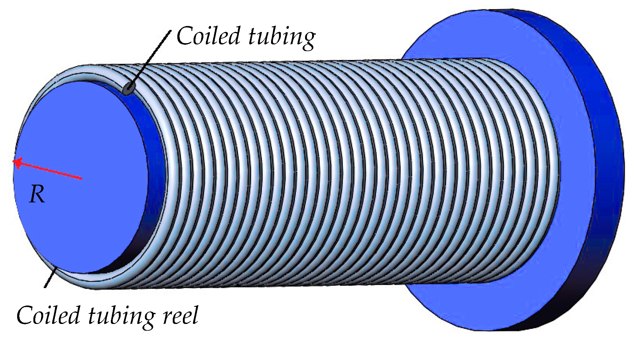
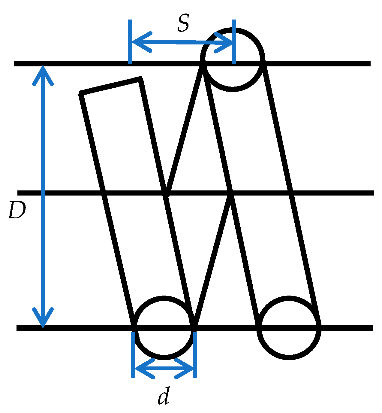
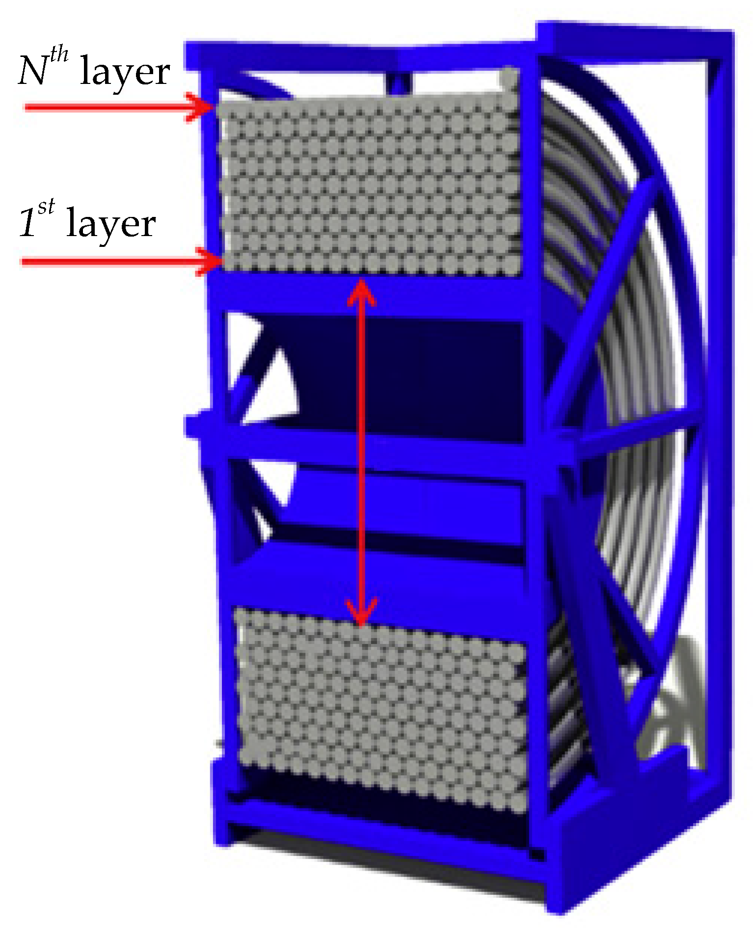
2.2. Geometric Configurations and Computational Conditions

Coiled tubing is wrapped around a drum, sticking one end into the gooseneck guide. The control cabin controls the tubing, which enters the well through the injector head. A one-layer coiled tubing wound drum is shown in Figure 1. Due to the repeatability of coiled tubing on a drum, one-unit spiral section was selected as the research object, as shown in Figure 2. The inside diameter of the helical tubing is d and its radius is r, the diameter of the drum is D and its radius is R, and the pitch is S. Since the coils are tightly wound, the pitch is equal to the inner diameter of the CT, that is, S = d. The curvature ratio is defined as the diameter ratio of the spiral tube to the tubing reel, that is, λ = d/D = r/R.

The diameters of the coils and tubing are the same as in flow experiments conducted by Zhou [9,32,33]; six numerical models of M1-M6 were established, as shown in

Table 1. Geometric dimensions of coils and tubing.

Model	CT Diameter	Coil Diameters	Curvature Ratio
	d (in)	D (in)	d/D
M1	0.435	3.6	0.010
M2	0.435	1.8	0.019
M3	0.435	1.2	0.031
M4	0.435	0.5	0.076
M5	0.810	48	0.017
M6	1.532	82	0.018

. In this study, water and gas were used as the working fluids to compare experimental results. The rheological properties of the fluids are based on sample data at ambient temperature. Water was selected as the liquid phase, with a density of 998.200 kg/m³ and viscosity of 1.003 mPa·s. Air was selected as the gas phase, with a density of 1.205 kg/m³ and viscosity of 0.0181 mPa·s.

The meshing of the helical tube was stretched to a 3D block by a 2D auxiliary block and swept; next, structured meshing was performed. The inlet region was divided into O-shaped meshing, as shown in Figure 3. The near-wall region was processed with a refined mesh and treated using non-equilibrium wall functions. The non-slip boundary condition was used at the tubing wall. The inlet and outlet boundaries were set as velocity- and pressure-outlet boundary conditions, respectively. CFD simulations of two-phase flow in CT were performed with Fluent 19.0 to study the flow behavior of the gas and liquid phases [34]. The finite volume method was used to discretize the governing equations, and the phase-coupled SIMPLE scheme discretized the pressure–velocity coupling [35]. To obtain satisfactory accuracy and better convergence, all results were simulated using a constant time step of 1 × 10⁻⁵ s on an HP-T7000 workstation (1 T hard disk, 8 GB RAM, and 3.6 GHz CPU).

3. Results and Discussion

3.1. Mesh Sensitivity Study

Primary studies were carried out to investigate the variation in simulation results, using grid number variation for pressure drop under different gas void fractions. Taking M2 as an example, with the inlet velocity v_in set as 5 m/s, the pressure drops along the tubing at four grid sizes (85,000, 98,000, 113,000, and 126,000) is shown in Figure 4. When the number of grids increases from 85,000 to 98,000, the pressure drop increases by 15.2%; when the grid size increases from 98,000 to 113,000, the pressure drop changes by 1.2%; and when the grid size increases from 113,000 to 126,000, the pressure drop changes by 0.8%. It was observed that when grids number increases from 98,000 to 126,000, the pressure drop does not change significantly. Considering calculation accuracy and computational cost, the number of grid points was finally chosen as 98,000.

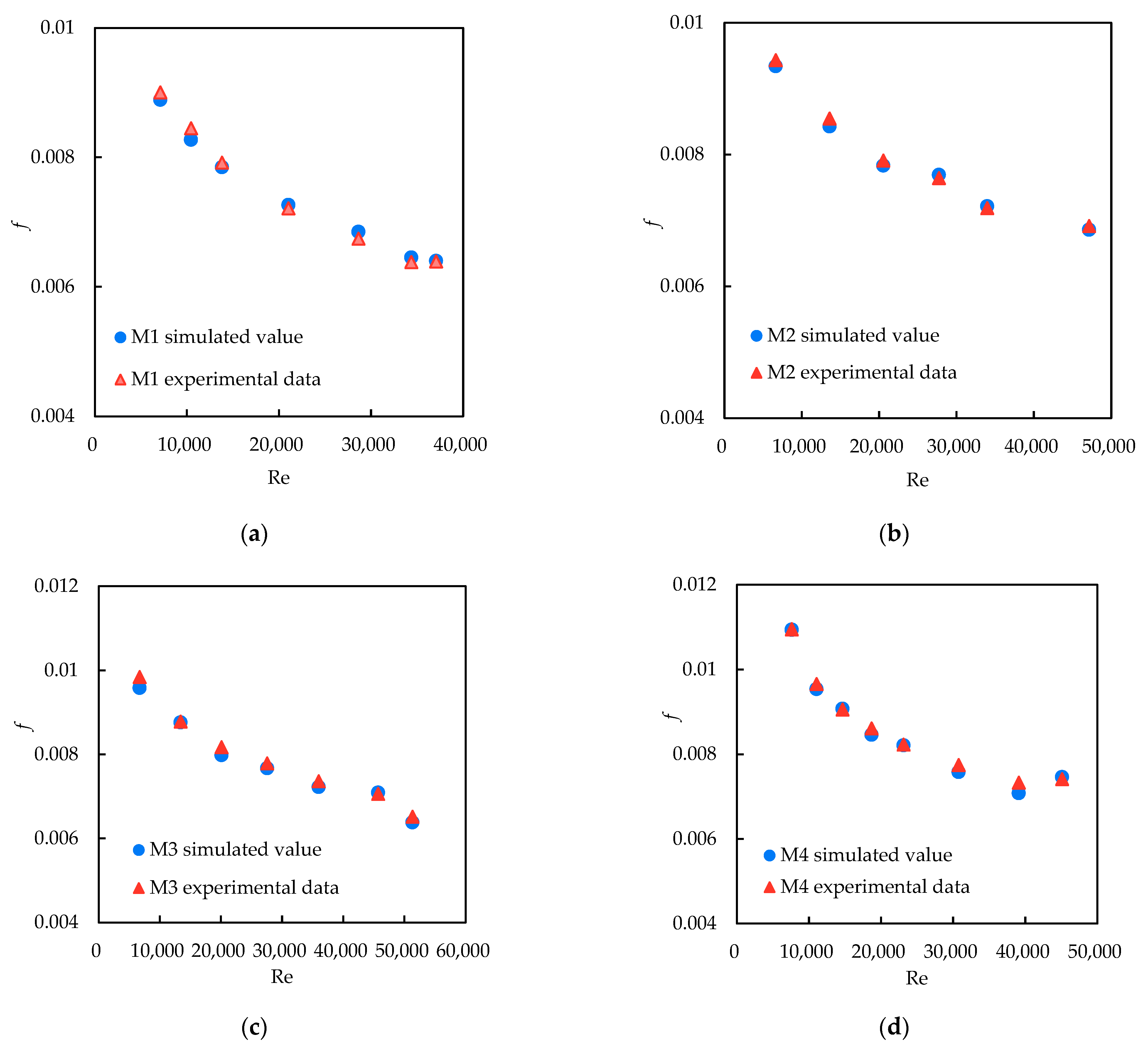
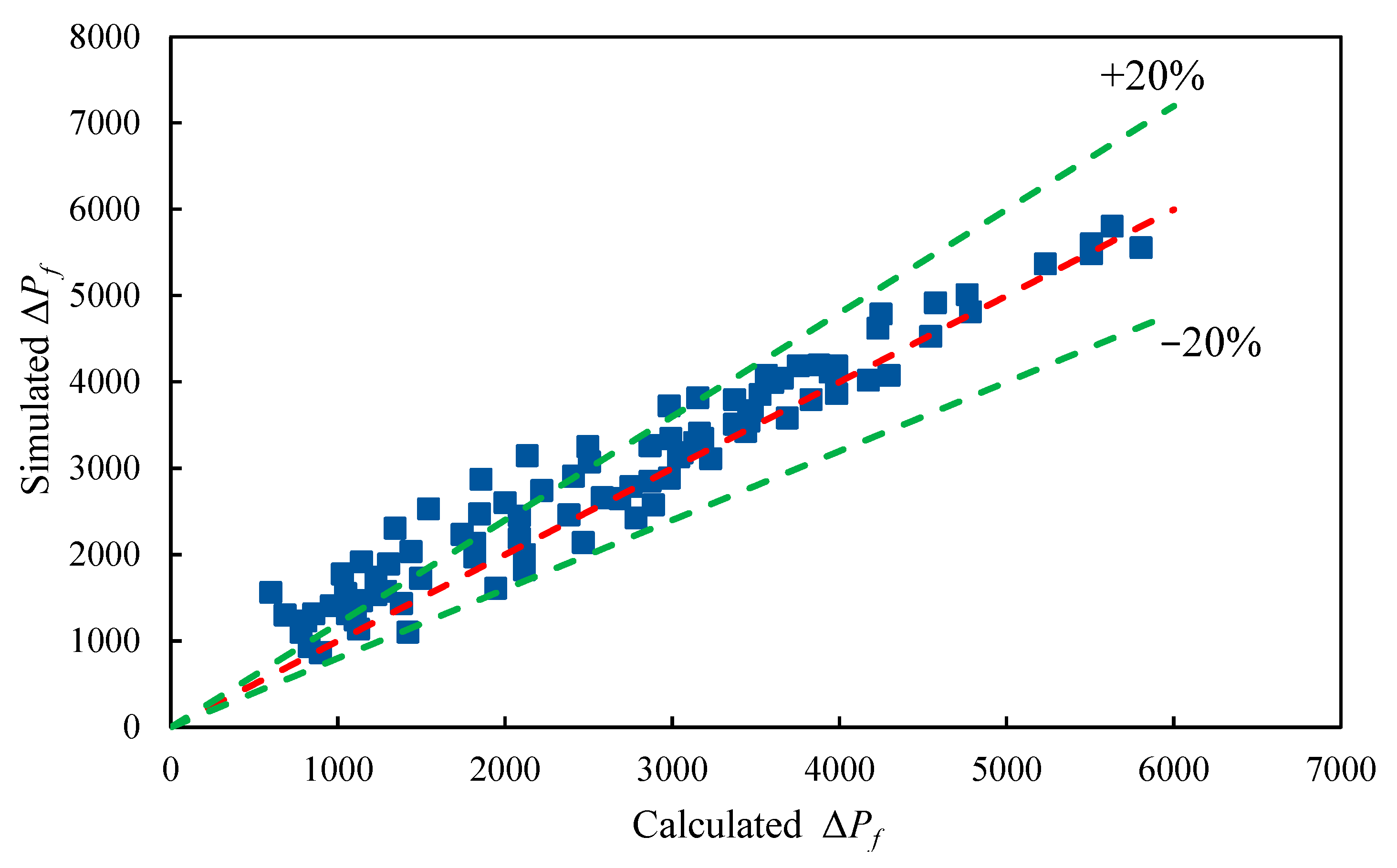
3.2. Model Validation between Simulations and Experiments

Comparisons of simulated and measured values of the Fanning friction factor, f, in CT for M1-M6 tubing sizes are shown in Figure 5 as a function of the Reynolds number, Re. In Zhou’s experiment, water was used as the fluidizing agent, the density was 998.20 kg/m³, and the viscosity was 1.003 mPa·s. The Reynolds number was 5000 < Re <230,000, and flow was turbulent in tubing for all sizes in the experiment.

For Newtonian fluids, the friction factor, f, for smooth CT in turbulent flow can be calculated by Srinivasan’s correlation [36]:

$$f=\frac{0.084{\left(\raisebox{1ex}{$d$}\!\left/ \!\raisebox{-1ex}{$D$}\right.\right)}^{0.2}}{{\mathrm{Re}}^{0.2}}$$

(8)

Equation (10) is suitable for a curvature ratio range of 0.0097 < d/D < 0.135.

The critical Reynolds number, Re_c, can be expressed as

$${\mathrm{Re}}_{\mathrm{c}}=2100\left[1+12{\left(\raisebox{1ex}{$d$}\!\left/ \!\raisebox{-1ex}{$D$}\right.\right)}^{0.5}\right]$$

(9)

Figure 5 shows that the friction factor decreases as the Reynolds number increases, which is consistent with the trend of experimental data. Average error (Avg. error) and standard deviation (RMS) are used to characterize the error between simulation and experimental values to verify the validity of the numerical model. Average error (Avg. error) reflects the difference between simulated results and experimental value, and can be expressed as:

$$Avg.error=\frac{1}{\mathrm{n}}{\displaystyle {\sum }_{\mathrm{n}=1}^{\mathrm{n}}\left|\frac{\mathsf{\Delta }{P}_{EXP}}{\mathsf{\Delta }{P}_{SIM}}-1\right|}$$

(10)

where $\mathsf{\Delta }{P}_{EXP}$ is the experimental data for the pressure drop, $\mathsf{\Delta }{P}_{SIM}$ is the simulated value of the pressure drop, and n is the number of data points.

Standard deviation (RMS) reflects the stability of the error between simulated and experimental data, and can be given as follows:

$$RMS=\sqrt{\frac{{\displaystyle {\sum }_{\mathrm{n}=1}^{\mathrm{n}}{(erro{r}_i-Avg.error)}^2}}{\mathrm{n}-1}}$$

(11)

The average error and standard deviation between simulation and experimental values for M1-M6 coiled tubing are shown in

Table 2. Average error and standard deviation between simulation and experimental value for M1-M6 coiled tubing.

Model	Avg. Error	RMS
M1	1.11%	0.0029
M2	0.88%	0.0035
M3	1.57%	0.0053
M4	1.21%	0.0060
M5	0.72%	0.0027
M6	1.43%	0.0063

. We can see from the data that the maximum average error and standard deviation are 2.14% and 0.006, respectively. The simulation results agree well with the experimental results, which proves that the established simulation model and the above numerical method can simulate fluid flow in coiled tubing.

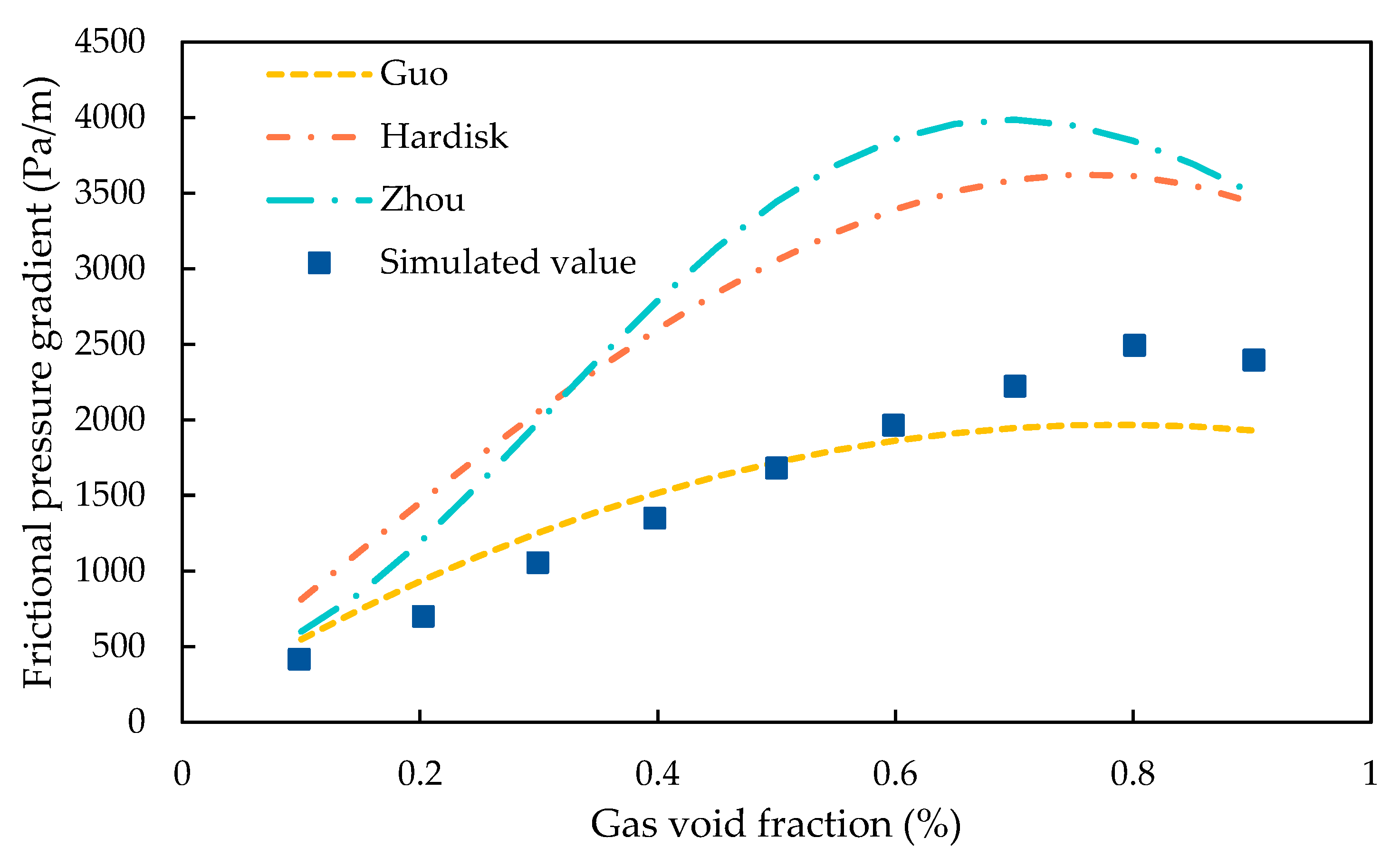
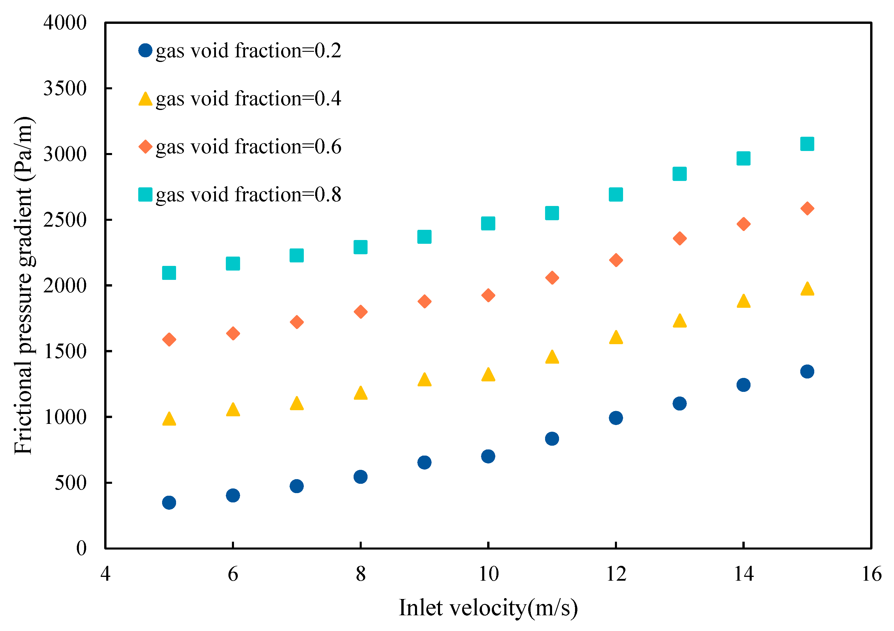
3.3. Effect of Gas Void Fraction on Frictional Pressure Losses

The inlet velocity was set to 10 m/s, and gas void fraction was set to 0.1, 0.2, 0.3..., and 0.9, respectively. Flow in M1, M5 and M6 coiled tubing was simulated. Due to the different tubing sizes in M1, M5 and M6, the influence of the CT size on flow is eliminated, and the effect of the gas void fraction on frictional pressure gradient is analyzed, as Figure 6 shows. The frictional pressure gradient of gas–liquid two-phase flow in CT has a parabolic relationship with the gas void fraction. When the gas void fraction is small, the frictional pressure gradient increases rapidly as void fraction increases, and when gas void fraction increases to 0.8, the frictional pressure gradient decreases with the increase in void fraction. This phenomenon is also verified by the empirical formula’s variation law of frictional pressure drop. The numerical simulation results are compared with the calculated values of Guo [21], Hardik [24], and Zhao [25] correlations, as Figure 7 shows. We can see from both numerical results and empirical formula calculation that with the increase in gas void fraction, there will be a “peak value” of frictional pressure drop. This peak value appears roughly between 0.6 and 0.8 of the gas void fraction. This peak phenomenon is because when the gas mass content is too high, the two gas–liquid phases will have apparent slippage, and the frictional pressure drop gradient will begin to decline. Moreover, the simulated values of frictional pressure drop are in good match with GUO correlation results.

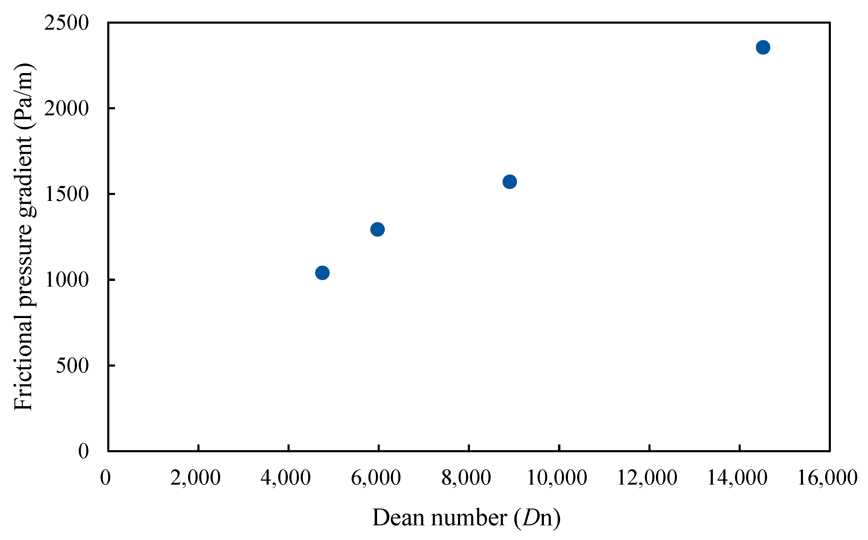
3.4. Effect of Curvature Ratio on Frictional Pressure Losses

The curvature ratios of M1, M2, M3 and M4 are 0.01, 0.019, 0.031 and 0.076, respectively. The gas void fraction was set to 0.2, 0.4, 0.6 and 0.8, respectively, and flow in M1, M2, M3 and M4 coiled tubing was simulated. Figure 8 shows the frictional pressure gradient with curvature ratio at four different gas void fractions.

It is found that as the curvature ratio increases, the frictional pressure gradient increases. This is because when the fluid flows in coiled tubing, the fluid is constantly thrown to the outer tubing wall and interacts with the outer tubing wall, resulting in friction loss. The frictional pressure drop is mainly affected by tubing roughness, fluid viscosity and the interaction between the fluid and the outer wall. In CT operation, once the tubing and drilling fluid is selected, the properties of the tubing roughness and drilling fluid cannot be changed. Only tubing curvature will affect secondary flow intensity, that is, the extent of interaction between the fluid and tubing outside wall. Therefore, the strength of the secondary flow is the main factor affecting the frictional pressure drop of flow in variable curvature tubes.

The influence of secondary flow intensity on frictional pressure drop can be described by the Dean number, and the Dean number of two-phase flow can be calculated by Polsongkram’s correlation [37]:

$${D\mathrm{n}}_{\mathrm{tp}}={\mathrm{Re}}_{\mathrm{tp}}{\left(\frac{d}{D}\right)}^{0.5}$$

(12)

Reynolds number of two-phase flow can be expressed as

$${\mathrm{Re}}_{\mathrm{tp}}={\mathrm{Re}}_{\mathrm{l}}+{\mathrm{Re}}_{\mathrm{g}}\left(\frac{{\mu }_{\mathrm{g}}}{{\mu }_{\mathrm{l}}}\right){\left(\frac{{\rho }_{\mathrm{l}}}{{\rho }_{\mathrm{g}}}\right)}^{0.5}$$

(13)

where Dn_tp and Re_tp are the Dean number and Reynolds number of two-phase flow, respectively. Re_l, μ_l and ρ_l are Reynolds numbers, viscosity and density of liquid phase, respectively. Re_g, μ_g and ρ_g are Reynolds numbers, viscosity and gas phase density, respectively.

Using Equations (14) and (15), we can calculate the Dean number of two-phase at a gas void fraction of 0.2, 0.4, 0.6 and 0.8 under different curvature ratios, and the average value is called the average Dean number of two-phase. The average value of the friction pressure gradient under the same Dean number is called the average frictional pressure gradient. Figure 9 shows the average frictional pressure gradient with the average Dean number of two-phase with a curvature ratio of 0.012.

When the average Dean number of two-phase is 4800, the average frictional pressure gradient is 1040 Pa/m. When the Dean number increases to 8900, the average frictional pressure drop gradient is 1577 Pa/m, increasing by 430 Pa/m. Secondary flow intensity has little influence on friction. When the average Dean number increases to 14,500, the average frictional pressure gradient increases to 2350 Pa/m, and the difference is 1310 Pa/m. At this time, the influence of secondary flow on frictional pressure drop becomes significant.

3.5. Effect of Inlet Velocity on Frictional Pressure Losses

The inlet velocity was set to 5 m/s, 6 m/s, 7 m/s, and… 15 m/s; the gas void fraction was set to 0.2, 0.4, 0.6 and 0.8, respectively; and flow in M2 coiled tubing was simulated. The frictional pressure gradient with inlet velocity at four different gas void fractions is shown in Figure 10. As inlet velocity increases, the frictional pressure gradient increases. This is because as inlet velocity increases, the volume flow rate of fluid flow through the tube increases, the interaction between fluid and tube wall is strengthened, and the centrifugal force effect becomes noticeable. The intensity of secondary flow increases with the increase in inlet velocity. As a result, the frictional pressure gradient of gas–liquid two-phase flow in the spiral tubes increases.

3.6. Development of Friction Factor Correlation for Gas–Liquid Two-Phase Flow in CT

The frictional pressure drop of single-phase gas and liquid can be calculated from:

$${\left(\frac{\mathrm{d}{P}_f}{\mathrm{d}Z}\right)}_g=f_g\frac{v_g^2}{2d}$$

(14)

$${\left(\frac{\mathrm{d}{P}_f}{\mathrm{d}Z}\right)}_l=f_l\frac{v_l^2}{2d}$$

(15)

where ${\left(\frac{\mathrm{d}{P}_f}{\mathrm{d}Z}\right)}_g$ and ${\left(\frac{\mathrm{d}{P}_f}{\mathrm{d}Z}\right)}_l$ are the frictional pressure gradient of gas and liquid phases, respectively.

Because there is no friction factor correlations suitable for gas flow in a spiral tube, the friction factor for single-phase turbulent flow was calculated by Blasius’s equation:

$$f=\frac{0.3164}{{\mathrm{Re}}^{0.25}}$$

(16)

A factor Y is defined as:

$$Y=\raisebox{1ex}{${\left(\frac{\mathrm{d}{P}_f}{\mathrm{d}Z}\right)}_g$}\!\left/ \!\raisebox{-1ex}{${\left(\frac{\mathrm{d}{P}_f}{\mathrm{d}Z}\right)}_l$}\right.=\frac{f_g}{f_l}\frac{{\rho }_{\mathrm{l}}}{{\rho }_{\mathrm{g}}}$$

(17)

By substituting Equation (16) into Equation (17), we can get:

$$Y={\left(\frac{{\rho }_{\mathrm{l}}}{{\rho }_{\mathrm{g}}}\right)}^{1.25}{\left(\frac{{\mu }_{\mathrm{g}}}{{\mu }_{\mathrm{l}}}\right)}^{0.25}$$

(18)

Based on Chisholm B’s coefficient method [38], the two-phase friction factor correlation was obtained as follows:

$${\phi }_{tp}^2=1+\phi (Y-1)=1+\phi \left[{\left(\frac{{\rho }_{\mathrm{l}}}{{\rho }_{\mathrm{g}}}\right)}^{1.25}{\left(\frac{{\mu }_{\mathrm{g}}}{{\mu }_{\mathrm{l}}}\right)}^{0.25}-1\right]$$

(19)

According to the influencing factors of frictional pressure drop analyzed above, we selected gas void fraction α, curvature ratio λ (d/D), and inlet velocity v for regression analysis. Using the multivariate nonlinear regression statistics method, the correction factor, $\phi$, can be obtained as follows:

$$\phi =2.35{\left(\frac{d}{D}\right)}^{0.75}{\left(\frac{v}{100}\right)}^{0.33}{\alpha }^{1.3}{\left(1-\alpha \right)}^{0.3}+{\alpha }^{2.5}$$

(20)

The following frictional pressure correlation for gas–liquid two-phase flow can be proposed as

$$\mathsf{\Delta }{P}_{ftp}={\phi }_{{}_{tp}}^2\mathsf{\Delta }{P}_l$$

(21)

where the frictional pressure of single-phase fluid can be expressed as

$$\mathsf{\Delta }{P}_l=f_l\frac{L}{d}\frac{v_l^2}{2}$$

(22)

Correlation is used to predict the friction factor of fluid flowing in a spiral tube:

$$f_l=\frac{1}{4}{\left(\frac{d}{D}\right)}^{0.5}\left\{0.029+0.304{\left[\mathrm{Re}{\left(\frac{d}{D}\right)}^2\right]}^{-0.25}\right\}$$

(23)

The comparison of the calculated results of Equation (21) with simulated data is shown in Figure 11. The maximum deviation between the calculated and simulated value is 39%, and 82.3% of simulated data are within the error range of 20% of calculated results. The reason for the error of the established frictional pressure correlation is that there is no model to accurately predict gas–liquid two-phase flow parameters. Moreover, no friction factor correlation is fit for the flow of gases in a spiral tube [39]. In this study, we use the Blasius formula for turbulent flow of Newtonian fluid in smooth straight tubes to calculate the Reynolds number of the gas; and the liquid phase friction factor is calculated by an empirical equation which does not consider the tubing roughness. All these will cause calculation error of the model. Therefore, it is necessary to conduct further studies on the hydrodynamic characteristics of CT. A frictional pressure drop model is expected to establish what the influence of tubing roughness and curvature ratio are.

During CT operation, tubing is wound on a drum in multiple layers, and the curvature ratio of different layers is different, as shown in Figure 12. From 3.4, we know that the curvature ratio significantly influences frictional pressure of flow. Therefore, we have further modified Equation (21) to meet the prediction of frictional pressure for gas–liquid two-phase flow in multiple wound tubing.

The curvature ratio of each layer of tubing can be calculated as

$$\lambda =\frac{d}{D}=\frac{2d}{4D+\left(2N-1\right)d}$$

(24)

where N is the number of tubing layers.

The tubing length of each layer can be described as follows:

$$L_N=\frac{L_r}{d}\pi \left[D+(2N-1)d\right]=L_r\pi \left[\frac{D}{d}+(2N-1)\right]$$

(25)

where L_N is the tubing length of the N^th layer, and L_r is the width of the reel.

Then we can calculate the single-phase flow frictional pressure of the Nth layer as:

$$\mathsf{\Delta }{P}_{lN}=f_{lN}\frac{L_N}{d}\frac{v_{{}^{lN}}^2}{2{\rho }_l}$$

(26)

Thus, we can obtain the frictional pressure correlation of multi-layer tubing as:

$$\mathsf{\Delta }{P}_{ftpN}={\left({\phi }_{{}_{tp1}}^2\mathsf{\Delta }{P}_{l1}\right)}_{1^{st}layer}+{\left({\phi }_{{}_{tp2}}^2\mathsf{\Delta }{P}_{l2}\right)}_{2^{nd}layer}+\dots \dots +{\left({\phi }_{tpN}^2\mathsf{\Delta }{P}_{lN}\right)}_{n^{th}layer}$$

(27)

4. Conclusions

The flow behavior of gas and liquid in spiral tubes is simulated using the Eulerian–Eulerian two-phase fluid model approach with the standard k-ε model for the turbulent viscosity of the gas–liquid fluid. The effects of gas void fraction, curvature ratio and inlet velocity on frictional pressure losses in CT were analyzed.

The frictional pressure drop gradient has a parabolic relationship with the gas void fraction, and the frictional pressure losses reach their peak when gas void fraction is 0.8. The frictional pressure drops increase with the increase in curvature ratio. As gas–liquid inlet velocity increases, the secondary flow strength increases, and the flow friction in the spiral section increases. Based on fluid mechanics theory, multivariate nonlinear statistics are conducted on simulation results, and friction factor correlation for gas–liquid two-phase flow in CT is established. Based on error analysis of the developed equation, we recommend that further research on the hydrodynamic characteristics of CT should be conducted to study the combined influence of tubing roughness and curvature ratio. The research results are expected to provide a theoretical basis for hydraulic design. It is worth noting that the simulation in this study does not consider the influence of the rheological properties of non-Newtonian fluids. Future studies will focus on the influence of the shear stress and shear dilution of non-Newtonian fluids on the flow behavior of the gas–liquid flow.

References

1. Walton, I.C.; Gu, H. Hydraulics Design in Coiled Tubing Drilling. In Proceedings of the SPE Gulf Coast Section/ICoTA North American Coiled Tubing Roundtable, Conroe, TX, USA, 26–28 February 1996. [Google Scholar]
2. McCann, R.C.; Isias, C.G. Frictional Pressure Loss during Turbulent Flow in Coiled Tubing. In Proceedings of the SPE Gulf Coast Section/ICoTA North American Coiled Tubing Roundtable, Conroe, TX, USA, 26–28 February 1996. [Google Scholar]
3. Azouz, I.; Shah, S.N.; Vinod, P.S.; Lord, D.L. Experimental Investigation of Frictional Pressure Losses in Coiled Tubing. SPE Prod. Facil. 1998, 13, 91–96. [Google Scholar] [CrossRef]
4. Rao, B.N. Friction Factors for Turbulent Flow of Non–Newtonian Fluids in Coiled Tubing. In Proceedings of the SPE/ICoTA Coiled Tubing Conference and Exhibition, Houston, TX, USA, 9–10 April 2002. [Google Scholar]
5. Medjani, B.; Shah, S.N. A New Approach for Predicting Frictional Pressure Losses of Non–Newtonian Fluids in Coiled Tubing. In Proceedings of the Rocky Mountain Regional/Low–Permeability Reservoirs Symposium and Exhibition, Denver, Colorado, 12–15 March 2000. [Google Scholar]
6. Willingham, J.D.; Shah, S.N. Friction Pressures of Newtonian and Non–Newtonian Fluids in Straight and Reeled Coiled Tubing. In Proceedings of the SPE/ICoTA Coiled Tubing Roundtable, Houston, TX, USA, 5–6 April 2000. [Google Scholar]
7. Shah, S.N.; Zhou, Y. An Experimental Study of the Effects of Drilling Solids on Frictional Pressure Losses in Coiled Tubing. In Proceedings of the SPE Production and Operations Symposium, Oklahoma City, Oklahoma, 24–27 March 2001. [Google Scholar]
8. Zhou, Y.; Shah, S.N. New Friction Factor Correlations for Non–Newtonian Fluid Flow in Coiled Tubing. SPE Drill. Completion. 2006, 21, 68–76. [Google Scholar] [CrossRef]
9. Hou, X.; Zheng, H.; Zhao, J.; Chen, X. Analysis of Circulating System Frictional Pressure Loss in Microhole Drilling with Coiled Tubing. Open Pet. Eng. J. 2014, 7, 22–28. [Google Scholar] [CrossRef] [Green Version]
10. Jain, S.; Singhal, N.; Shah, S.N. Effect of Coiled Tubing Curvature on Friction Pressure Loss of Newtonian and Non–Newtonian Fluids–Experimental and Simulation Study. In Proceedings of the SPE Annual Technical Conference and Exhibition, Houston, TX, USA, 26–29 September 2004. [Google Scholar]
11. Zhou, Y.; Shah, S.N. Non–Newtonian Fluid Flow in Coiled Tubing: Theoretical Analysis and Experimental Verification. In Proceedings of the SPE Annual Technical Conference and Exhibition, San Antonio, TX, USA, 29 September–2 October 2002. [Google Scholar]
12. Shah, S.; Zhou, Y.; Bailey, M.; Hernandez, J. Correlations to Predict Frictional Pressure Loss of Hydraulic–Fracturing Slurry in Coiled Tubing. SPE Prod. Oper. 2009, 24, 381–395. [Google Scholar] [CrossRef]
13. Pereira, C.E.G.; da Cruz, G.A.; Pereira Filho, L.; Justino, L.R.; Paraiso, E.C.H.; Rocha, J.M.; Calçada, L.A.; Scheid, C.M. Experimental Analysis of Pressure Drop in the Flow of Newtonian Fluid in Coiled Tubing. J. Pet. Sci. Eng. 2019, 179, 565–573. [Google Scholar] [CrossRef]
14. Oliveira, B.R.; Leal, B.C.; Pereira Filho, L.; Borges, R.F.d.O.; Paraíso, E.d.C.H.; Magalhães, S.d.C.; Rocha, J.M.; Calçada, L.A.; Scheid, C.M. A Model to Calculate the Pressure Loss of Newtonian and Non–Newtonian Fluids Flow in Coiled Tubing Operations. J. Pet. Sci. Eng. 2021, 204, 10864. [Google Scholar] [CrossRef]
15. Martinelli, R.C.; Nelson, D.B. Prediction of Pressure Drop during Forced–Circulation of Boiling Water. Trans. ASME 1948, 70, 695–702. [Google Scholar]
16. Lockhart, R.W.; Martinelli, R.C. Proposed Correlation of Data for Isothermal Two–Phase Two Component Flow in Pipes. Chem. Eng. Prog. 1949, 45, 39–45. [Google Scholar]
17. Akagawa, K.; Sakaguchi, T.; Ueda, M. Study on a Gas– Liquid Two– Phase Flow in Helically Coiled Tubes. Bull. JSME 1971, 14, 564–571. [Google Scholar] [CrossRef] [Green Version]
18. Bi, Q.; Chen, T.; Luo, Y.; Zheng, J.; Jing, J. Frictional Pressure Drop of Steam–Water Two–Phase Flow in Helical Coils with Small Helix Diameter of HTR–10. Chin. J. Nucl. Sci. Eng. 1996, 3, 208–213. [Google Scholar] [CrossRef]
19. Xin, R.C.; Awwad, A.; Dong, Z.F.; Ebadian, M.A. An Experimental Study of Single–Phase and Two–Phase Flow Pressure Drop in Annular Helicoidal Pipes. Int. J. Heat Fluid Flow 1997, 18, 482–488. [Google Scholar] [CrossRef]
20. Santini, L.; Cioncolini, A.; Lombardi, C.; Ricotti, M. Two–Phase Pressure Drops in a Helically Coiled Steam Generator. Int. J. Heat Mass Tran. 2008, 51, 4926–4939. [Google Scholar] [CrossRef]
21. Guo, L.; Feng, Z.; Chen, X. An Experimental Investigation of the Frictional Pressure Drop of Steam–Water Two–Phase Flow in Helical Coils. Int. J. Heat Mass Tran. 2001, 44, 2601–2610. [Google Scholar] [CrossRef]
22. Colombo, M.; Cammi, A.; Guédon, G.R.; Inzoli, F.; Ricotti, M.E. CFD Study of an Air–Water Flow inside Helically Coiled Pipes. Prog. Nucl. Energy 2015, 85, 462–472. [Google Scholar] [CrossRef] [Green Version]
23. Cioncolini, A.; Santini, L. Two–Phase Pressure Drop Prediction in Helically Coiled Steam Generators for Nuclear Power Applications. Int. J. Heat Mass Tran. 2016, 100, 825–834. [Google Scholar] [CrossRef] [Green Version]
24. Hardik, B.K.; Prabhu, S.V. Boiling Pressure Drop and Local Heat Transfer Distribution of Helical Coils with Water at Low Pressure. Int. J. Therm. Sci. 2017, 114, 44–63. [Google Scholar] [CrossRef]
25. Zhao, H.; Li, X.; Wu, X. New Friction Factor Equations Developed for Turbulent Flows in Rough Helical Tubes. Int. J. Heat Mass Tran. 2016, 95, 525–534. [Google Scholar] [CrossRef]
26. Xiao, Y.; Hu, Z.; Chen, S.; Gu, H. Experimental Study of Two–Phase Frictional Pressure Drop of Steam–Water in Helically Coiled Tubes with Small Coil Diameters at High Pressure. Appl. Therm. Eng. 2018, 132, 18–29. [Google Scholar] [CrossRef]
27. Wu, J.; Li, X.; Liu, H.; Zhao, K.; Liu, S. Calculation Method of Gas–Liquid Two–Phase Boiling Heat Transfer in Helically–Coiled Tube Based on Separated Phase Flow Model. Int. J. Heat Mass Tran. 2020, 161, 114381. [Google Scholar] [CrossRef]
28. Wu, J.; Li, Z.; Li, S.; Chen, Y.; Liu, S.; Xia, C.; Chen, Y. Numerical Simulation Research on Two–Phase Flow Boiling Heat Transfer in Helically Coiled Tube. Nucl. Eng. Des. 2022, 395, 111827. [Google Scholar] [CrossRef]
29. Gidaspow, D. Multiphase Flow and Fluidization: Continuum and Kinetic Theory Descriptions; Academic Press: Cambridge, MA, USA, 2012. [Google Scholar]
30. Rzasa, M.R.; Czapla–Nielacna, B. Analysis of the Influence of the Vortex Shedder Shape on the Metrological Properties of the Vortex Flow Meter. Sensors 2021, 21, 4697. [Google Scholar] [CrossRef] [PubMed]
31. Wilcox, D.C. Turbulence Modeling for CFD; DCW Industries: La Canada, CA, USA, 1998. [Google Scholar]
32. Zhou, Y.; Shah, S.N. Rheological Properties and Frictional Pressure Loss of Drilling, Completion, and Stimulation Fluids in Coiled Tubing. J. Fluid Eng.–T ASME 2004, 126, 153–161. [Google Scholar] [CrossRef]
33. Zhou, Y. Theoretical and Experimental Studies of Power–Law Fluid Flow in Coiled Tubing; University of Oklahoma: Norman, Oklahoma, 2006. [Google Scholar]
34. Fluent. Ansys Fluent User’s Guide; ANSYS, Inc. Release 19.0: Canonsburg, PA, USA, 2018. [Google Scholar]
35. Ogugbue, C.C.; Shah, S.N. Laminar and Turbulent Friction Factors for Annular Flow of Drag–Reducing Polymer Solutions in Coiled–Tubing Operations. SPE Drill. Completion 2011, 26, 506–518. [Google Scholar] [CrossRef]
36. Srinivasan, P.S.; Nandapurkar, S.S.; Holland, S.S. Friction Factors for Coils. Trans. Inst. Chem. Eng. 1970, 48, 156–161. [Google Scholar]
37. Wongwises, S.; Polsongkram, M. Condensation Heat Transfer and Pressure Drop of HFC–134a in a Helically Coiled Concentric Tube–in–Tube Heat Exchanger. Int. J. Heat Mass Transf. 2006, 49, 4386–4398. [Google Scholar] [CrossRef]
38. Chisholm, D. Two–Phase Flow in Pipelines and Heat Exchangers; Longmen Group Ltd.: London, UK, 1983. [Google Scholar]
39. Bharath, R. Coiled Tubing Hydraulics Modeling; CTES, L. C: Conroe, TX, USA, 1999. [Google Scholar]
Figure 1. Schematic diagram of one-layer CT.
Energies 15 08969 g001
Figure 2. Geometric parameters of a unit of helical tube.
Energies 15 08969 g002
Figure 3. Computational grid of a unit of helical tube.
Energies 15 08969 g003
Figure 4. Simulated pressure drop along the tubing at four grid sizes.
Energies 15 08969 g004
Figure 5. Comparison between simulated and experimental friction factor for M1-M6: (a) M1, (b) M2, (c) M3, (d) M4, (e) M5 and (f) M6.
Energies 15 08969 g005aEnergies 15 08969 g005b
Figure 6. Effects of a gas void fraction on frictional pressure drop.
Energies 15 08969 g006
Figure 7. Comparisons between simulations and calculations of Hardik, Guo, and Zhao correlations.
Energies 15 08969 g007
Figure 8. Frictional pressure gradient with curvature ratio at different gas void fractions.
Energies 15 08969 g008
Figure 9. Average frictional pressure gradient with average Dean number.
Energies 15 08969 g009
Figure 10. Frictional pressure gradient with inlet velocity at different gas void fractions.
Energies 15 08969 g010
Figure 11. Comparison of calculated frictional pressure with simulated data.
Energies 15 08969 g011
Figure 12. Schematic diagram of multi-layer coiled tubing drum.
Energies 15 08969 g012