Abstract
This study proposes a novel logarithm curve and operating time (LCOT) control strategy for a self-driving electric mobile robot. This new LCOT control strategy enables the mobile robot to speed up and slow down mildly when running longitudinally, turning left, turning right, and encountering an obstacle based on the relationship between the logarithm curve and operating time. This novel control strategy can enhance the comfort and stability of the self-driving electric mobile robot and reduce its vibrations and instabilities in the operation process. The proposed LCOT control strategy and the fixed duty cycle method were verified experimentally. The results showed that the LCOT control strategy spent 300 s running on a 3000 cm road, whereas the fixed duty cycle method spent 450 s. Because this novel method controls the acceleration and deceleration of the self-driving electric mobile robot gently and flexibly, the proposed LCOT control strategy has better working efficiency than the fixed duty cycle method. This novel control strategy is simple and easy to be implemented. As it can reduce the working load of the controller, increase system efficiency, and require low cost, it can be effectively used in a self-driving electric mobile robot.
1. Introduction
The development of automobiles has upgraded the quality of life in the 20th century. The performance, safety, and comfort of automobiles have improved greatly over this period. The automobile manufacturing cost decreased gradually, and most vehicles used fossil fuels during this period [1]. Since the late 20th century, hybrid electric vehicles have been gradually popularized [2]. Besides finding alternative energy sources, decreasing the greenhouse effect is important [3]. To combat global warming and extreme climate in the 21st century [4], many countries have implemented strategies and policies such as reducing coal consumption, reducing methane emissions, and popularizing zero-carbon-emission electric vehicles (EVs) [5]. Therefore, EVs are expected to be an important development for transportation in the 21st century. Electric vehicles include trains, subways, buses, automobiles, and motorcycles [6,7,8,9,10]. This study focuses on self-driving electric mobile robot control technology. With this control technology, the self-driving electric mobile robot can operate flexibly and stably, and the research horizon can be expanded to self-driving EVs in the future.
Many studies have discussed the control strategies for autonomous vehicles [11,12,13,14,15,16,17,18]. The advantages and disadvantages of these control strategies for autonomous vehicles are as follows: In 2020, Karnouskos proposed quantitative and ethical decision-making techniques for controlling the running vehicle during an accident to reduce the damage to persons and the vehicle, but a number of experiments are required to prove the safety of the ethical decision-making of the control mechanisms [11]. In 2021, Chowdhury et al. studied the combination of the Dempster–Shafer theory and logic operation, which enabled the vehicle to run safely and reliably. However, their control method requires complex operations, such as the internet of things (IoT), global positioning systems (GPS), onboard controllers, and logic control, which would make the control system more complex and generate burdens on the system control [12]. In 2021, Tian et al. proposed a joint account unloading and buffering method, which could predict the next running environment of the vehicle so that the vehicle could run safely and stably. However, telecommunication signals and vehicle trajectories are added to the offline control strategy. So, when other vehicles have a temporary accident, its control strategy requires additional protection mechanisms [13]. In 2021, Dzeparoska et al. proposed a self-driving electric car control system of intent refinement and learning, so that the vehicle could run on the road accurately and stably; but the intent refinement and learning are time-consuming [14]. In 2022, Ni et al. discussed the rapid deep-learning control strategy for image recognition when the vehicle is running. If the available roads and the timing of stops are provided accurately, the safety of the self-driving electric car is further enhanced. However, this control strategy requires a large number of images for analysis in order to achieve the best accuracy, which increases the design costs [15]. In 2020, Shi et al. developed a long-term and short-term memories (LSTM) network to improve LSTM, which has a grasshopper optimization algorithm. The method controls the behavior of the running vehicle so that the vehicle can run in the lane accurately and safely. However, this method has good performance only in going straight and lane change. Thus, more conditions need to be tested for enhancing its performance [16]. In 2020, Park et al. proposed the motor variable frequency control method for a railroad car. Although this method enhanced the system performance, it also increased the complexity of the control and required analysis of the motor parameters [17]. In 2012, Gupta et al. developed the motor fixed duty cycle method for electric cars. Their method can obtain good economics but has low controllability [18].
This study proposed a novel logarithm curve and operating time (LCOT) control strategy for the self-driving electric mobile robot. This new LCOT method controls the running of the self-driving electric mobile robot based on the relationship between the logarithm curve and operating time. The mobile robot achieved mild and stable acceleration while running in a straight line, right turn, and left turn. It can stop gently and stably when encountering an obstacle. The proposed control strategy can increase the running efficiency of the self-driving electric mobile robot through a gentle and flexible operation.
The proposed LCOT control strategy dominates the variable frequency control method and the fixed duty cycle method because of its high efficiency and low cost. This study compares the complexity, parameters, and speed of the three control strategies. Table 1 shows the comparison of three control strategies, which use the same quantity of infrared (IR) sensors [19]. The proposed LCOT control strategy performed better than the variable frequency control and fixed duty cycle methods in controlling the running speed of the self-driving electric mobile robot. The proposed LCOT control strategy is based on the relationship between the logarithm curve and operating time. It helps the mobile robot to accelerate and decelerate gently, thereby enhancing the comfort, stability, and performance of the self-driving electric mobile robot. The design based on the relationship between the logarithm curve and operating time is simple and easy to be implemented, so as to reduce the working load of the controller and increase the system efficiency. This method can be effectively used by the self-driving electric mobile robot.

Table 1.
Comparison of three control strategies.
The remaining work is structured as follows: First, the self-driving electric mobile robot system and architecture descriptions are presented in Section 2. Section 3 presents the proposed LCOT control strategy. Experimental results are discussed in Section 4. Finally, the concluding remarks showing the contribution of this study are listed in Section 5.
2. The Self-Driving Electric Mobile Robot System and Structure
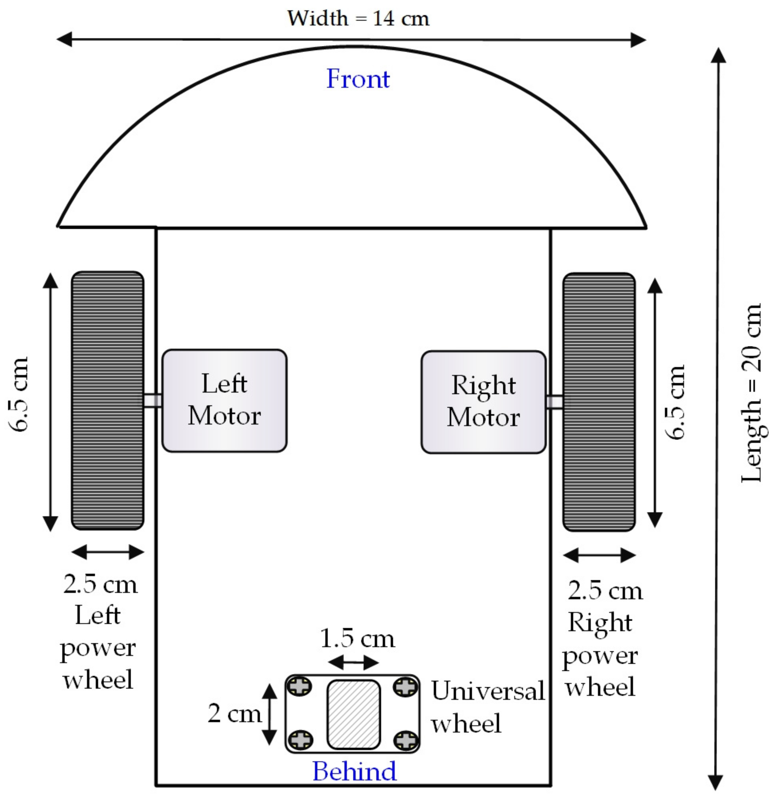
In this study, the self-driving electric mobile robot is a three-wheel type mobile robot [20]. It has one universal wheel and two power wheels, as shown in Figure 1. The universal wheel has a diameter of 2 cm with a width of 1.5 cm. The two power wheels have a diameter of 6.5 cm and a width of 2.5 cm. The mobile robot’s length, width, and height are 20 cm, 14 cm, and 12 cm, respectively. In this study, the advance and cornering of the self-driving electric mobile robot depend on the coordination of the left and right power wheels. Therefore, controlling the two power wheels in this study was important. Table 2 shows the component specifications of the self-driving electric mobile robot, including three infrared sensors, a microcontroller unit (MCU), a battery module, and two motors.
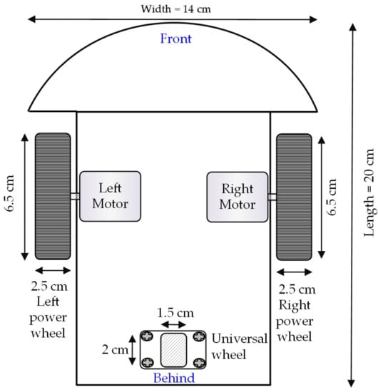
Figure 1.
Arrangement of wheels of the self-driving electric mobile robot.
Table 2.
Component specifications of the self-driving electric mobile robot.
Figure 2 illustrates the control system of the self-driving electric mobile robot. There are three important infrared sensors in this architecture diagram: the front infrared sensor, the left infrared sensor, and the right infrared sensor. The front infrared sensor detects whether there is any obstacle ahead of the self-driving electric mobile robot or not. The left and right infrared sensors detect the travel path of the self-driving electric mobile robot. The three infrared sensors transmit the detected signals to the MCU. The MCU receives the signals, operates according to the control strategy, and exports two sets of PWM signals to two driver ICs. Finally, the two driver ICs drive the left and right motors, respectively, according to the PWM signal received from MCU. Then, the self-driving electric mobile robot is actuated.
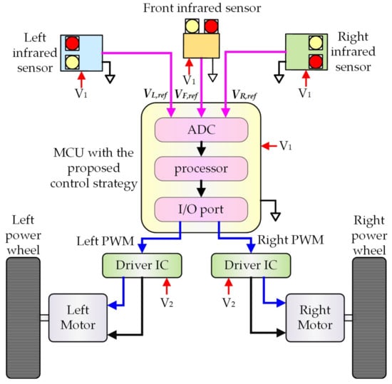
Figure 2.
Schematic diagram of the control system structure of the self-driving electric mobile robot.
Figure 3 shows the arrangement of various components of the self-driving electric mobile robot. Figure 3a is the top view of the self-driving electric mobile robot, showing the arrangement of three infrared sensors, two power wheels, a battery module, and a DC/DC converter. The MCU of the self-driving electric mobile robot is also illustrated. Figure 3b is the left view of the self-driving electric mobile robot. The positions of two infrared sensors, a battery module, two DC/DC converters, the left motor, the left power wheel, the universal wheel, and the MCU of the self-driving electric mobile robot can be observed. The 5 V output supplies of two DC/DC converters are V1 and V2, supplying power to various components, as shown in Figure 2.
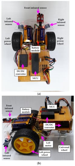
Figure 3.
Arrangement of various components of the self-driving electric mobile robot: (a) top view and (b) left view.
3. The Proposed Logarithm Curve and Operating Time Control Strategy
This traction control strategy is based on the relationship between the logarithm curve and operating time (LCOT) [21], as the logarithm curve has a stable curve variation (as shown in Equation (1)).
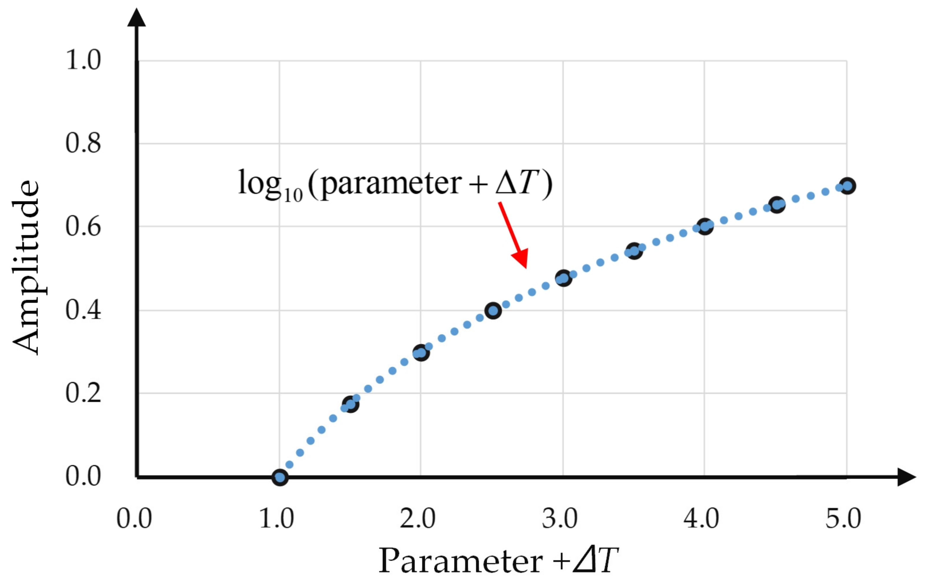
The self-driving electric mobile robot can speed up and turn stably based on the logarithm curve during straight running or cornering. The proposed LCOT control strategy is able to operate the self-driving electric mobile robot on the running path stably and effectively. Figure 4 shows the diagram of the Log10 curve, which illustrates the relationship between the amplitude and parameter + operation time ΔT; the X axis is a parameter + operation time (ΔT) and the Y axis is the amplitude.
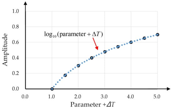
Figure 4.
Log10 curve depicting the relationship between the amplitude and parameter + operation time ΔT.
First, the self-driving electric mobile robot uses three infrared sensors to detect the work environment. It helps to make sure that there is any obstacle ahead of the self-driving electric mobile robot or not and that the path in the forward direction is straight. After receiving information from the infrared sensor, the MCU exports two duty cycles (dright and dleft) at a frequency of 200 kHz to drive two motors (as shown in Figure 2). This is based on the operation of Equation (2) during straight running. It helps to achieve a stable acceleration of the self-driving electric mobile robot.
where dright and dleft are the duty cycles of the right driver motor and left driver motor, respectively. The duty cycle (dright and dleft) range is 0.4~0.9, ΔT denotes operation time, and n1 of 0.25 is the compensation parameter. For setting the parameter a, it should be considered first that the logarithmic value of x should be negative between 0 and 1 (as shown in Equation (1)). Therefore, parameter a in Equation (2) should be greater than 1, so that dright and dleft provide positive values to drive the motors. This paper sets a to be 1.4, which fits the minimal value of 1.4 for dright and dleft so that the dual motors have sufficient power to drive the system.
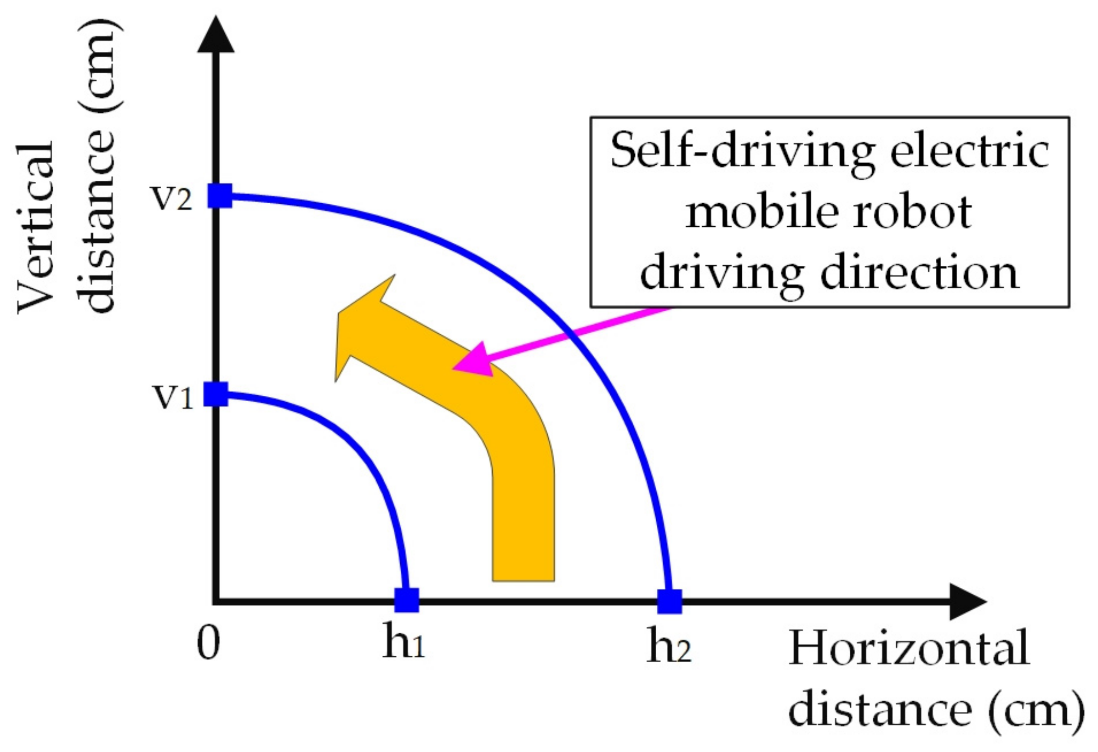
Second, the three infrared sensors of the self-driving electric mobile robot detect the work environment. When there is no obstacle ahead and the detected path is a left turn (as shown in Figure 5), where Figure 5 shows the curve diagram of the self-driving electric mobile robot taking a left turn; the X axis is horizontal distance, the Y axis is vertical distance, and the unit of both the axes are cm. At this point, this control strategy is based on the log10 curve (as shown in Figure 4). When the MCU receives the information from the infrared sensors and conducts a calculation by Equation (3), the MCU exports the duty cycle at a frequency of 200 kHz, and a drive signal is given to the left motor. When the mobile robot turns left, the right wheel’s running path is longer than that of the left wheel. Therefore, the right wheel should turn at a faster rate than the left wheel. At this point, it is calculated by Equation (4), and the MCU exports the duty cycle with a frequency of 200 kHz to give a drive signal to the right motor. Based on Figure 5 and Equations (3) and (4), the self-driving electric mobile robot can turn left stably. This control strategy is based on the log10 curve, operation time, compensation parameter n2, and the relationship between the radius of the inner curve (h1) and the radius of the outer curve (h2).
where dleft is the driver left motor duty cycle and the duty cycle (dleft) range is 0.2~0.36. ΔT denotes operation time and n2 is the compensation parameter with a value of 0.1. For setting the parameter b, firstly it should be considered that the logarithmic value of x should be negative between 0 and 1 (also as shown in Equation (1)). Therefore, parameter b in Equation (3) should be greater than 1 so that dright and dleft provide positive values to drive the motors. This paper sets b to be 1.25, which fits the minimal value of 0.2 for dleft to have sufficient power to drive the system.
where dright is the right driver motor’s duty cycle and the duty cycle (dright) has a range of 0.5~0.9. ΔT denotes operation time, n2 is the compensation parameter with a value of 0.1, h1 is the radius of the inner curve, and h2 is the radius of the outer curve. For setting the parameter b, the logarithmic value of x should be negative between 0 and 1 (as shown in Equation (1)). Therefore, parameter b in Equation (4) should be greater than 1 so that dright is positive to drive the motors. This paper sets b to be 1.25, which fits the minimal value of 0.5 for dright to have sufficient power to drive the system.
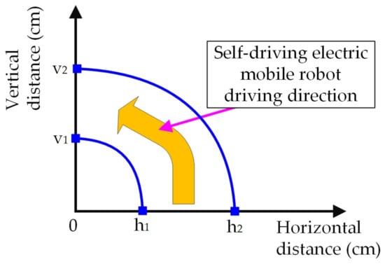
Figure 5.
Curve diagram of the self-driving electric mobile robot taking a left turn.
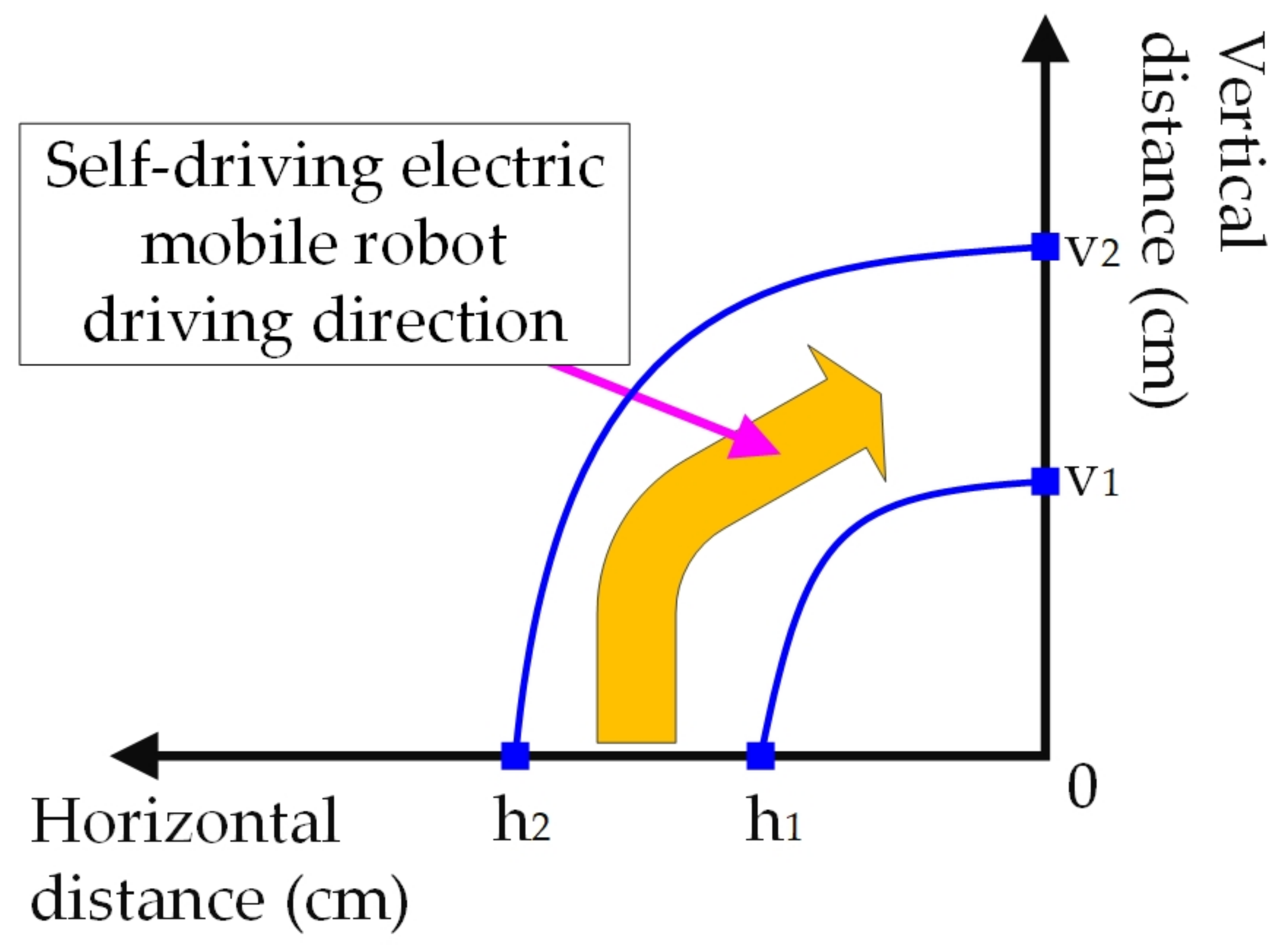
In addition, the three infrared sensors of the self-driving electric mobile robot detect the work environment. When there is no obstacle ahead and the detected path is a right turn (as shown in Figure 6). Figure 6 shows the curve diagram of the self-driving electric mobile robot with a curve on the right; the X axis is the horizontal distance, Y axis is vertical distance, and the unit of both the axes are cm. This control strategy is based on the log10 curve (as Figure 4). When the MCU receives the information from the infrared sensors, it calculates duty cycles using Equation (5). Then it exports the duty cycles at a frequency of 200 kHz, and a drive signal is given to the right motor. When the self-driving electric mobile robot is taking a right turn, the running path of the left wheel is longer than the right wheel. Therefore, the left wheel should turn faster than the right wheel. At this point, it is calculated by Equation (6). The MCU exports the duty cycle with a frequency of 200 kHz to give a drive signal to the left motor. Based on Figure 6 and Equations (5) and (6), the self-driving electric mobile robot can turn right stably. This control strategy is based on the log10 curve, operation time, compensation parameter n3, and the relationship between the radius of the inner curve (h1) and the radius of the outer curve (h2).
where dright is the duty cycle of the right driver motor and the duty cycle range is 0.2~0.36. ΔT denotes operation time, and n3 is the compensation parameter with a value of 0.1. For setting the parameter c, the logarithmic value of x should be negative between 0 and 1 as shown in Equation (1). Therefore, parameter c in Equation (6) should be greater than 1 so that dright is positive to drive the motors. This paper sets c to be 1.25, which fits the minimal value of 0.2 for dright to have sufficient power to drive the system.
where dleft is the left driver motor’s duty cycle and the duty cycle (dleft) range is 0.5 ~ 0.9. ΔT denotes operation time, n3 is the compensation parameter with a value of 0.1, h1 is the radius of the inner curve, and h2 is the radius of the outer curve. For setting the parameter c, the logarithmic value of x should be negative between 0 and 1 (as shown in Equation (1)). Therefore, parameter c in Equation (6) should be greater than 1 so that dleft is positive to drive the motors. This paper sets c to be 1.25, which fits the minimal value of 0.5 for dleft to have sufficient power to drive the system.
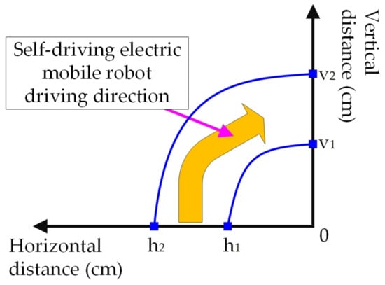
Figure 6.
Curve diagram of the self-driving electric mobile robot taking a right turn.
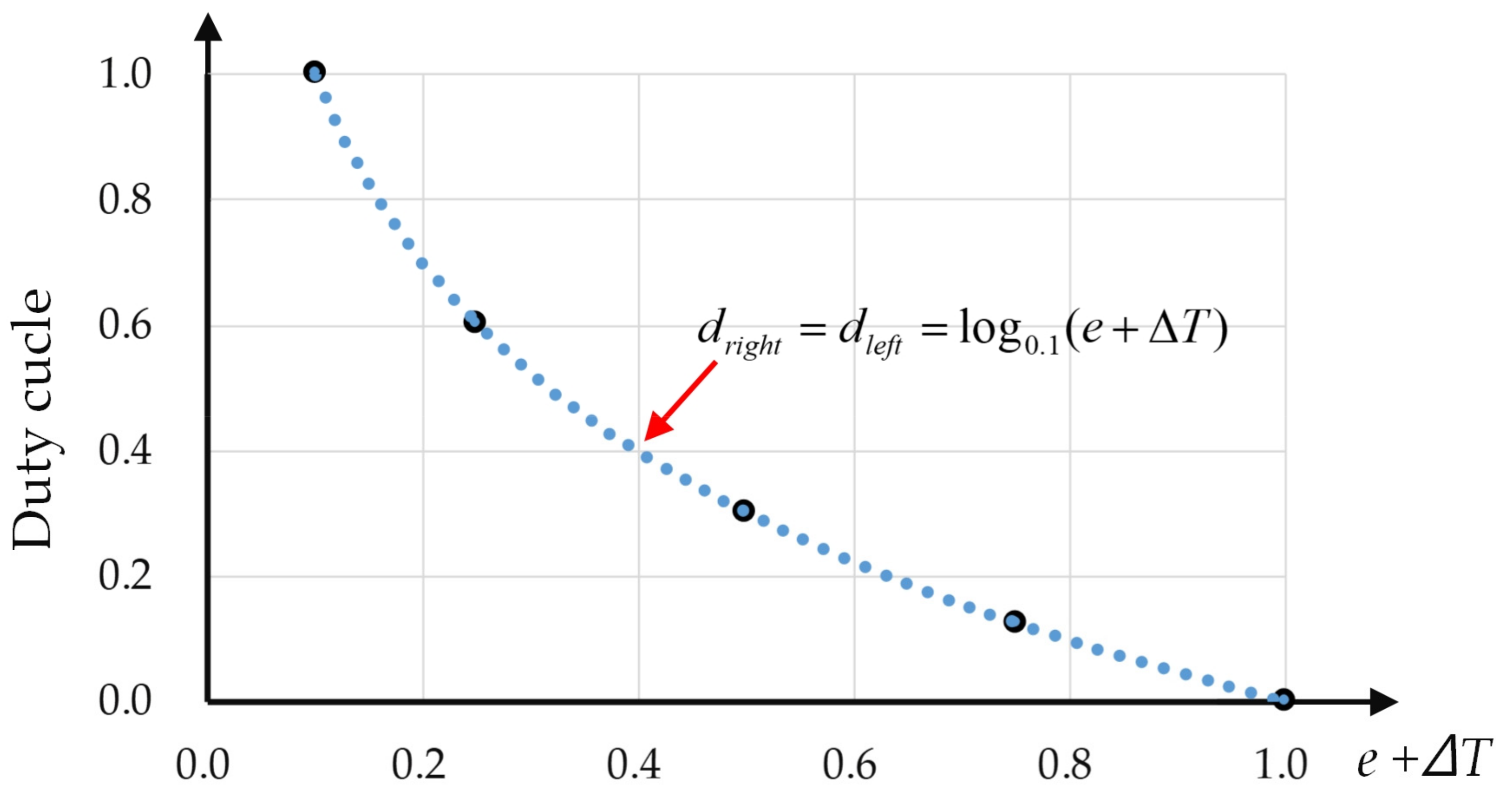
Finally, when an obstacle that is 10 cm ahead is detected, this control strategy is based on the log0.1 curve (as shown in Figure 7). Figure 7 shows the diagram of the Log0.1 curve which illustrates the relationship between the duty cycle and parameter e + operation time ΔT; the X axis is a parameter e + operation time (ΔT), and the Y axis is the duty cycle. When the MCU receives the information from the infrared sensors and conducts a calculation by Equation (7), the MCU exports two duty cycles (dright and dleft) at a frequency of 200 kHz to drive two motors (as shown in Figure 2). This helps the self-driving electric mobile robot to stably decelerate. The self-driving electric mobile robot stops at an operation time of 0.5 s from Equation (7).
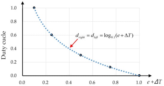
Figure 7.
Log0.1 curve depicting the relationship between the duty cycle and parameter e + operation time ΔT.
The duty cycle (dright and dleft) has a range of 0.1~0.3, and ΔT denotes operation time. The parameter e is set to be 0.5 to fit the maximal value of 0.3 for dright and dleft to gently stop the dual motors.
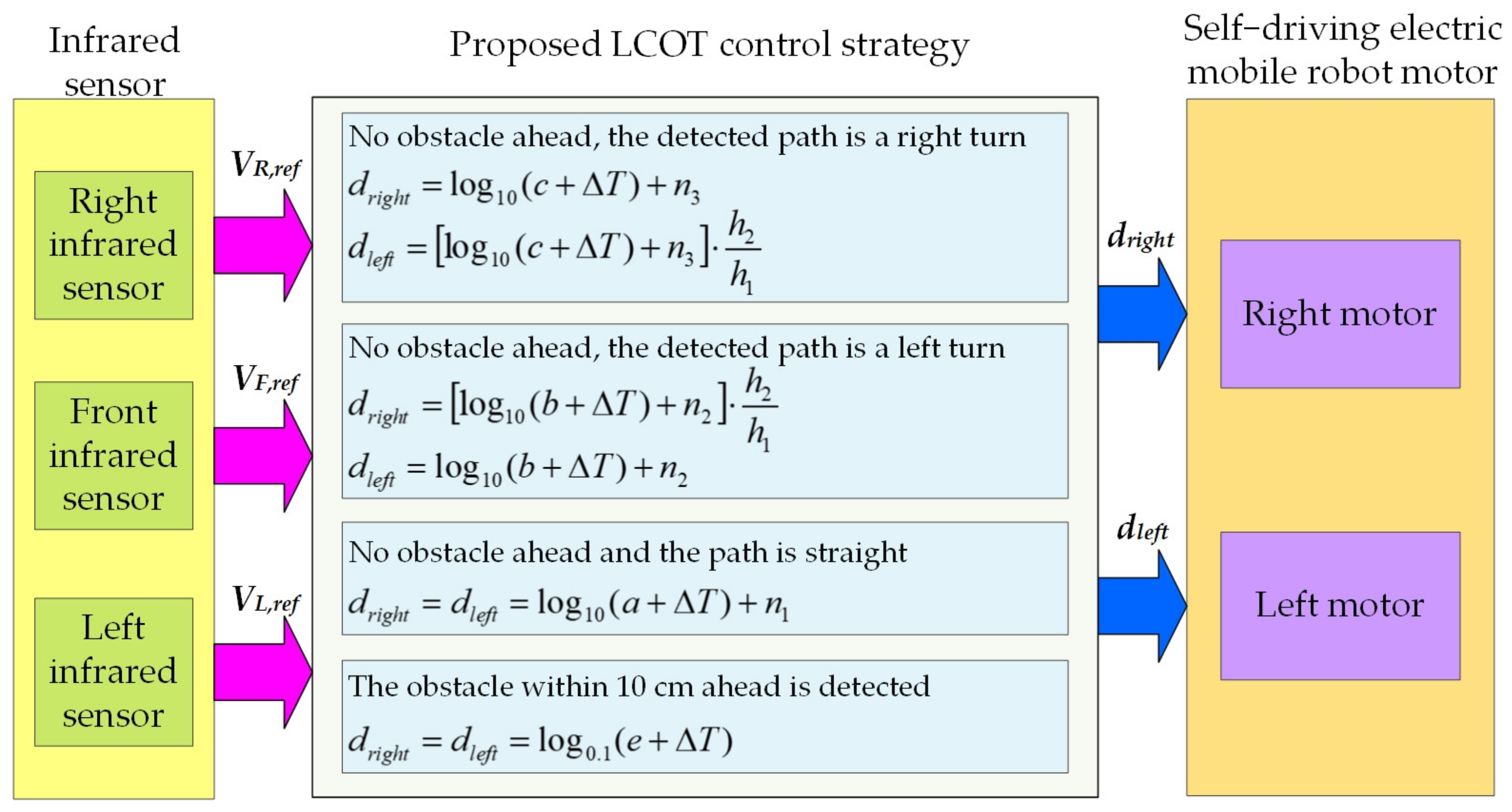
Figure 8 depicts the architecture diagram of the self-driving electric mobile robot control system [22]. First, three infrared sensors determine the driving path of the self-driving electric mobile robot and transmit this information to the MCU. Second, the MCU produces dleft and dright signals for the motor using the proposed LOCT control strategy. Third, dleft and dright drive the left motor and right motor, respectively. Finally, the self-driving electric mobile robot runs gently and flexibly. The specifications of the infrared sensor, MCU, motor, and ICs are mentioned in Table 2. The MCU confirmed to the three infrared sensors signal that the time is 100 us/time and the output PWM frequency is 200 kHz.

Figure 8.
Architecture diagram of the self-driving electric mobile robot control system.
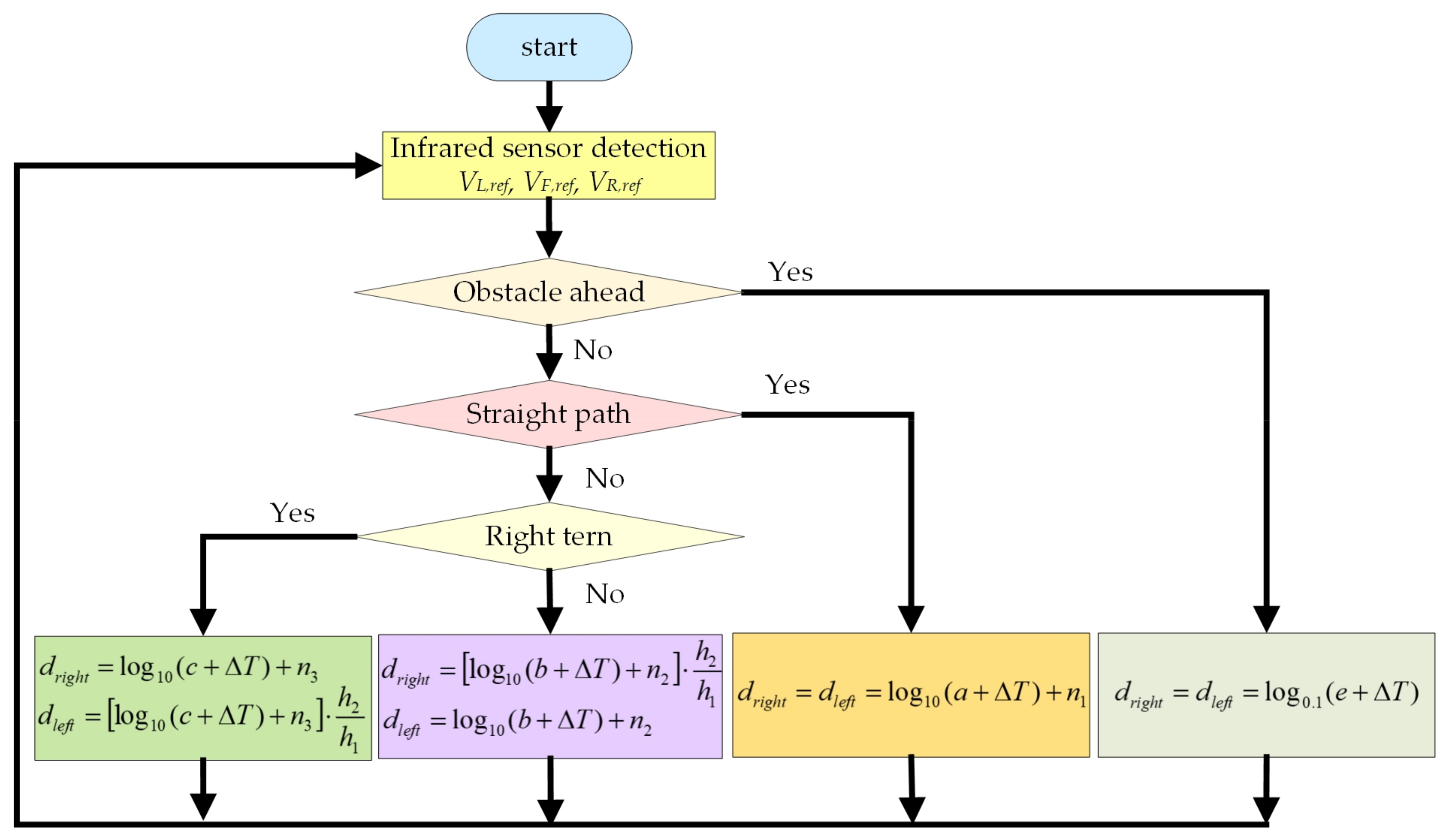
Figure 9 shows the flowchart of the proposed LCOT control strategy. First, the front, left, and right infrared sensors monitor the operational environment of the self-driving electric mobile robot. Second, the self-driving electric mobile robot detects an obstacle at a maximum distance of 10 cm ahead. Then, the MCU performs calculations using Equation (7). The MCU exports two sets of duty cycles (dleft and dright) to control two motors to decelerate and stop the mobile robot. The self-driving electric mobile robot confirms a straight running environment, and the MCU performs calculations using Equation (2). The MCU exports two sets of duty cycles (dleft and dright) to control two motors and to accelerate the self-driving electric mobile robot gently. If the running path is a right turn, the MCU calculates using Equations (5) and (6). Then, it exports two sets of duty cycles (dleft and dright) to drive the left and right motors individually for a stable right turn. If the running path is a left turn, the MCU calculates using Equations (3) and (4). It then exports two sets of duty cycles (dleft and dright) to drive the left and right motors, respectively. This makes the self-driving electric mobile robot turn left stably.
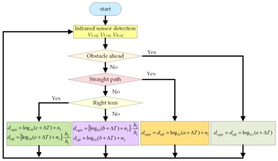
Figure 9.
Flowchart of the proposed LCOT control strategy.
Figure 10 shows the flowchart of the traditional fixed duty cycle method. First, the self-driving electric mobile robot uses the front, left, and right infrared sensors to monitor the environment. If it detects an obstacle within 10 cm ahead of the mobile robot, the MCU exports two sets of duty cycles (dleft = dright = 0.1) to control two motors for deceleration. In actual operation, the driving power of the MCU output duty cycle of 0.1 is low, and the mobile robot will stop. In a straight running environment, the MCU exports two sets of duty cycles (dleft = dright = 0.5) to drive two motors to keep the mobile robot on a straight path. If the running path is a right turn, the MCU exports two duty cycles, dleft = 0.6 and dright = 0.2. The left and right motors are provided with drive signals for a right turn. For a left turn, the MCU exports two duty cycles dleft = 0.2 and dright = 0.6. Then, the left and right motors are provided with drive signals to help the mobile robot turn left.
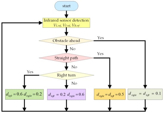
Figure 10.
Flowchart of the traditional fixed duty cycle method.
It is noted that though the traditional fixed duty cycle method might achieve the optimal duty cycle by continuous tuning according to engineering intuition, it is time- and labor-consuming. Contrarily, the proposed LCOT control strategy flexibly adopts the driving route and effectively accelerates, decelerates, and stops without any other devices. Therefore, the proposed LCOT control strategy is a simple and cost-effective design. The proposed LCOT control strategy and fixed duty cycle method are compared in Section 4, and their efficiency, reliability, and stability are further verified.
4. Experimental Results
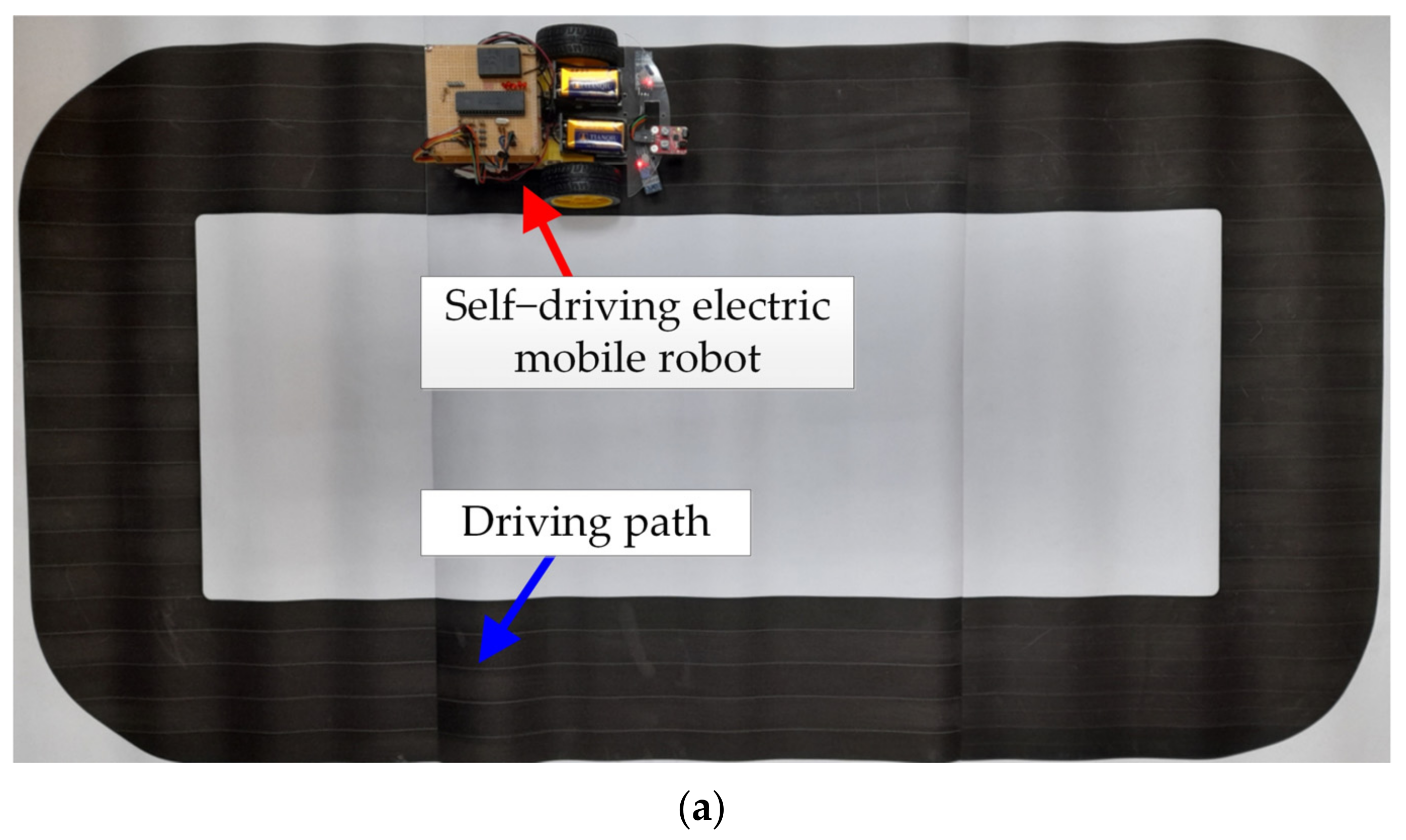
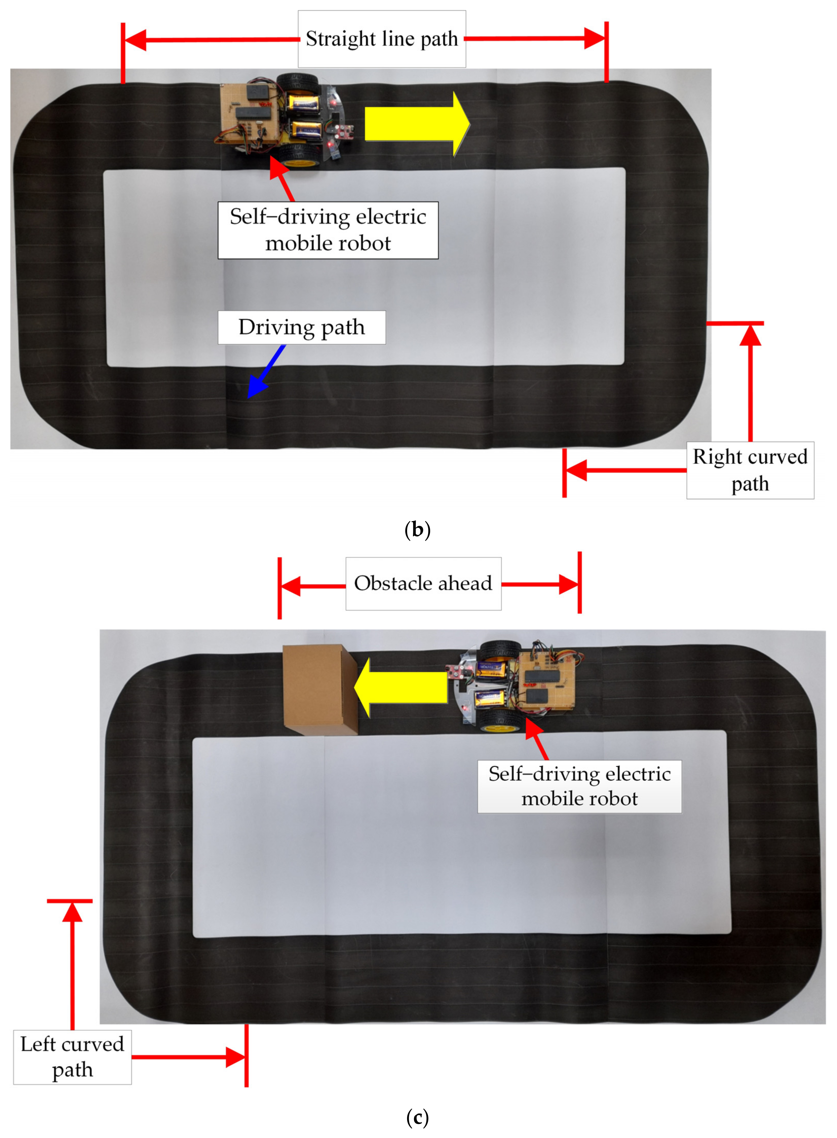
Figure 11 shows the actual self-driving electric mobile robot and the driving path of the test. Figure 11a shows the general view of the annular path, in which the overall length of the path is 300 cm with a width of 15 cm. The self-driving electric mobile robot was operated on this path. Figure 11b shows the straight line and right-curved path of the test path. Figure 11c shows an obstacle ahead and the left-curved path which has been used in this test. The proposed LCOT control strategy was tested using this path to prove its operational stability and reliability. The efficiency was compared with the traditional fixed duty cycle method for the self-driving electric mobile robot. The experimental results show that the proposed LCOT control strategy has better efficiency than the fixed duty cycle method (as shown in Figure 12, Figure 13, Figure 14 and Figure 15 and Table 3).
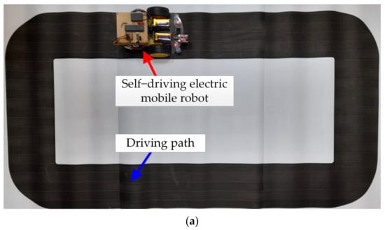
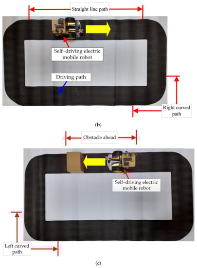
Figure 11.
Stereogram of the self-driving electric mobile robot and driving path: (a) overall view, (b) schematic diagram of a straight line path and right turn, and (c) schematic diagram of an obstacle ahead and the left turn.
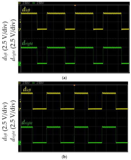
Figure 12.
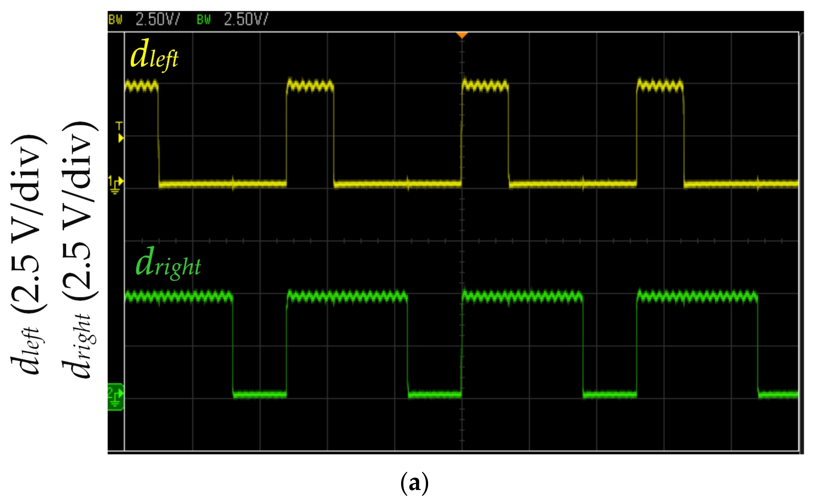
Measured MCU output dleft and dright waveforms during straight-line running: (a) with proposed LCOT control strategy and (b) with fixed duty cycle method. (The horizontal axis: 2 μs.)


Figure 13.
MCU output dleft and dright waveforms during left turning: (a) with proposed LCOT control strategy and (b) with fixed duty cycle method. (The horizontal axis: 2 μs.)
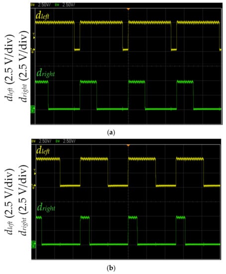
Figure 14.
MCU output dleft and dright waveforms during right turning: (a) with proposed LCOT control strategy and (b) with fixed duty cycle method. (The horizontal axis: 2 μs.)
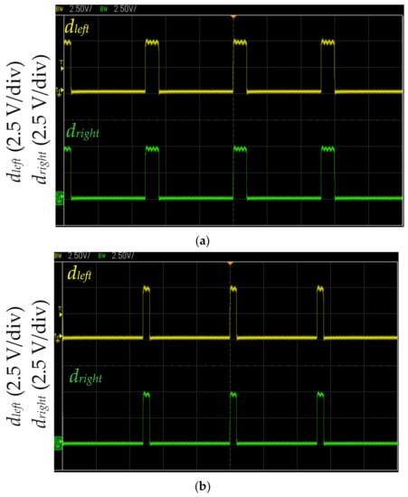
Figure 15.
MCU output dleft and dright waveforms of an obstacle ahead of the self-driving electric mobile robot: (a) with proposed LCOT control strategy and (b) with fixed duty cycle method. (The horizontal axis: 2 μs.)
Table 3.
Characteristics comparison of the two methods.
Figure 12 shows the measured MCU output dleft and dright waveforms during straight-line running. dleft and dright drive the left and right motors, respectively. Figure 12a shows the straight line path identified by three infrared sensors of the self-driving electric mobile robot (as shown in Figure 9 and Figure 11b). The proposed LCOT control strategy calculates dleft and dright according to Equation (2). When the straight-going operation time of the self-driving electric mobile robot is ΔT = 1.2 s, dleft and dright are 0.65 (frequency of 200 kHz). The proposed LCOT control strategy could perform acceleration in the straight line path to increase the working efficiency. As the proposed LCOT control strategy is based on the relationship between the logarithm curve and operation time, the acceleration is mild and stable. Figure 12b shows the straight-line driving path identified by three infrared sensors. The MCU produces duty cycles dleft and dright of 0.5 with a frequency of 200 kHz (as shown in Figure 10). The fixed duty cycle method is fixed for the self-driving electric mobile robot to run in the path at a constant speed. However, this method would result in poor work efficiency (as shown in Table 3).
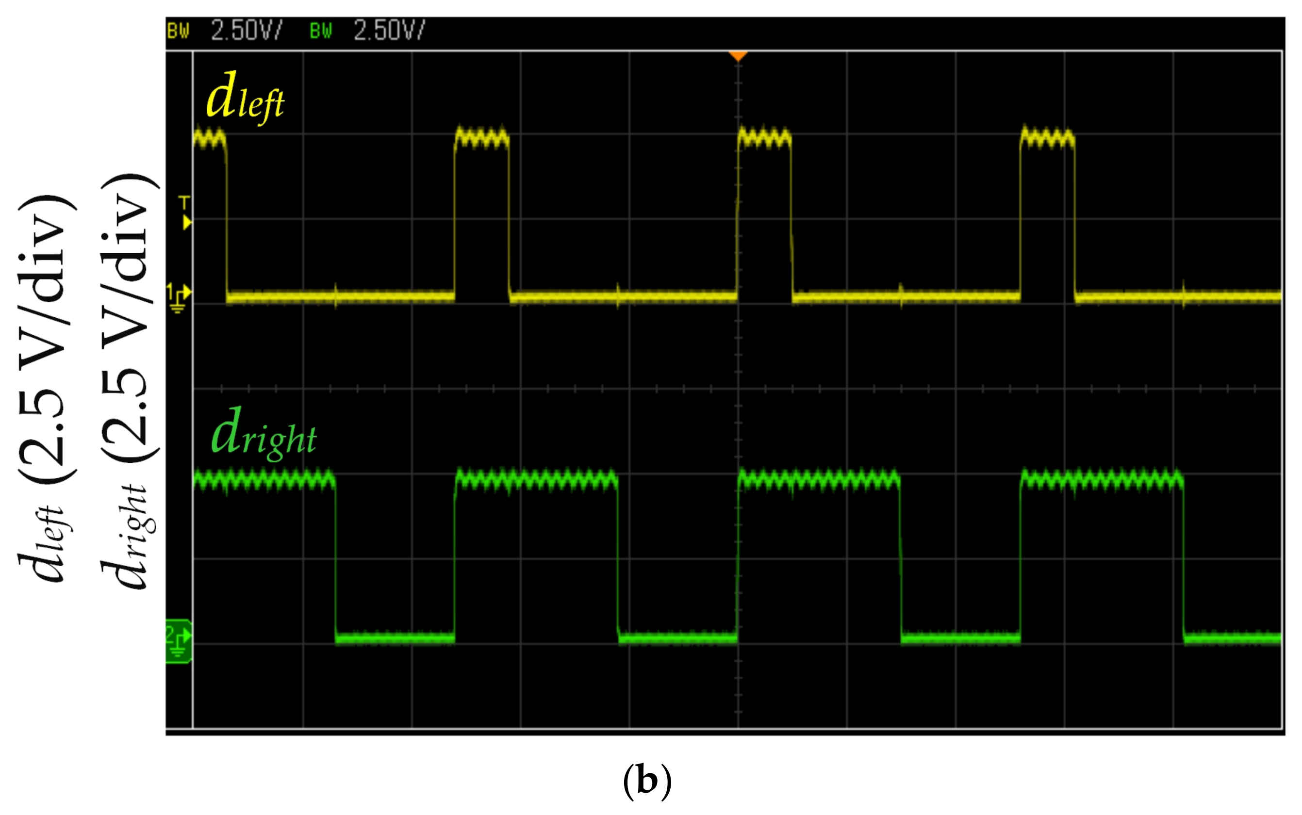
Figure 13 shows the measured MCU output dleft and dright waveforms during left turning. The dleft and dright drive the left and right motors, respectively. Figure 9, Figure 11c, and Figure 13a show the identified left-curved path. The proposed LCOT control strategy calculates dleft and dright according to Equations (3) and (4). When the left turning operation time of the self-driving electric mobile robot is ΔT = 0.27 s, dleft and dright are 0.28 and 0.69, respectively (duty cycle frequency of 200 kHz). The proposed LCOT control strategy could control acceleration in the left-curved path to increase working efficiency. Furthermore, the proposed LCOT control strategy is based on the relationship between the logarithm curve and operation time, so the acceleration of the self-driving electric mobile robot is mild and stable. Figure 13b shows the left-curved path identified by three infrared sensors of the self-driving electric mobile robot. The MCU generates the duty cycles dleft and dright, which are 0.2 and 0.6, respectively, with a duty cycle frequency of 200 kHz (as shown in Figure 10). The fixed duty cycle method of the duty cycle is fixed so that the self-driving electric mobile robot could run on the path at a constant speed. While the mobile robot could be controlled on the driving path stably, this method would result in poor work efficiency (as shown in Table 3).
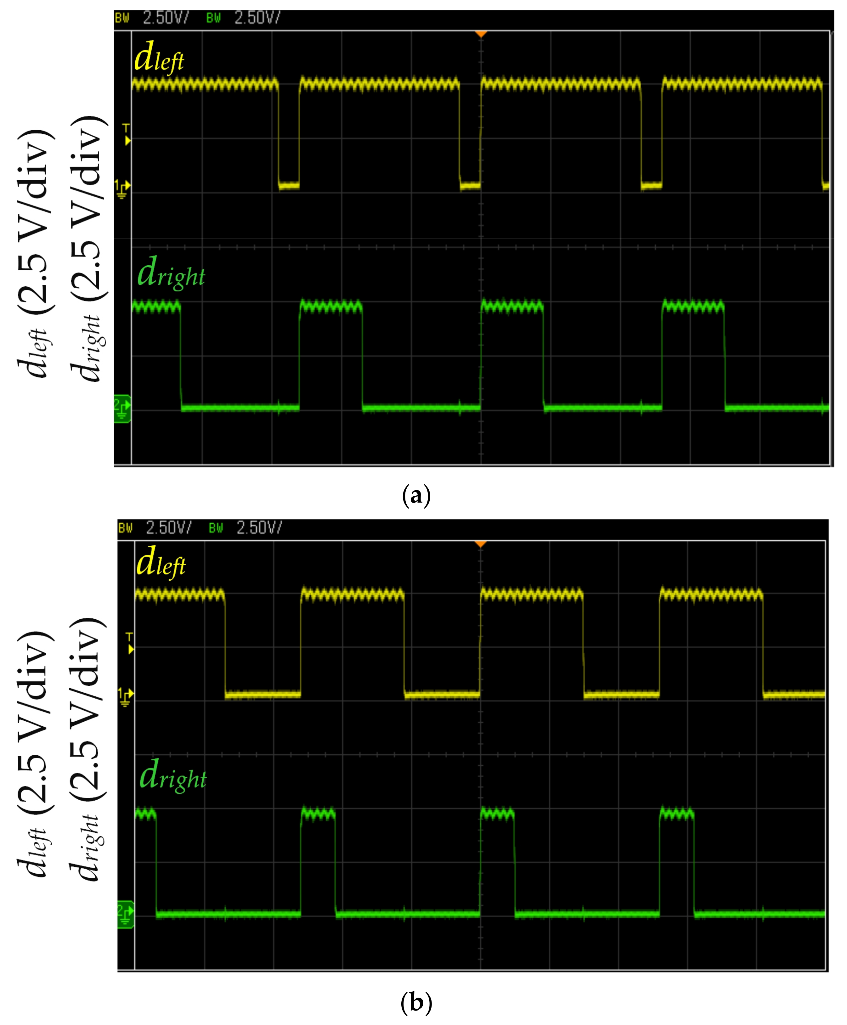
Figure 14 shows the measured MCU output dleft and dright waveforms during the right turning. The dleft and dright drive the left and right motors, respectively. Figure 14a shows the right-curved path identified by three infrared sensors. The proposed LCOT control strategy calculates dleft and dright according to Equations (5) and (6). When the right turning operation time of the self-driving electric mobile robot is ΔT = 0.57 s, the dleft and dright are 0.88 and 0.36, respectively (frequency of 200 kHz). The proposed LCOT control strategy could control acceleration in the right-curved path to increase working efficiency. The proposed LCOT control strategy is based on the relationship between the logarithm curve and operation time. Therefore, the acceleration is mild and maintains the stability of the self-driving electric mobile robot. Figure 14b shows the right-curved path identified by three infrared sensors of the self-driving electric mobile robot. The MCU produces the duty cycles dleft and dright, which are 0.6 and 0.2, respectively, with a frequency of 200 kHz (as shown in Figure 10). The fixed duty cycle method makes the self-driving electric mobile robot run in the path at a constant speed. While the mobile robot could be controlled on the driving path stably, this method would result in poor work efficiency of the self-driving electric mobile robot (as shown in Table 3).
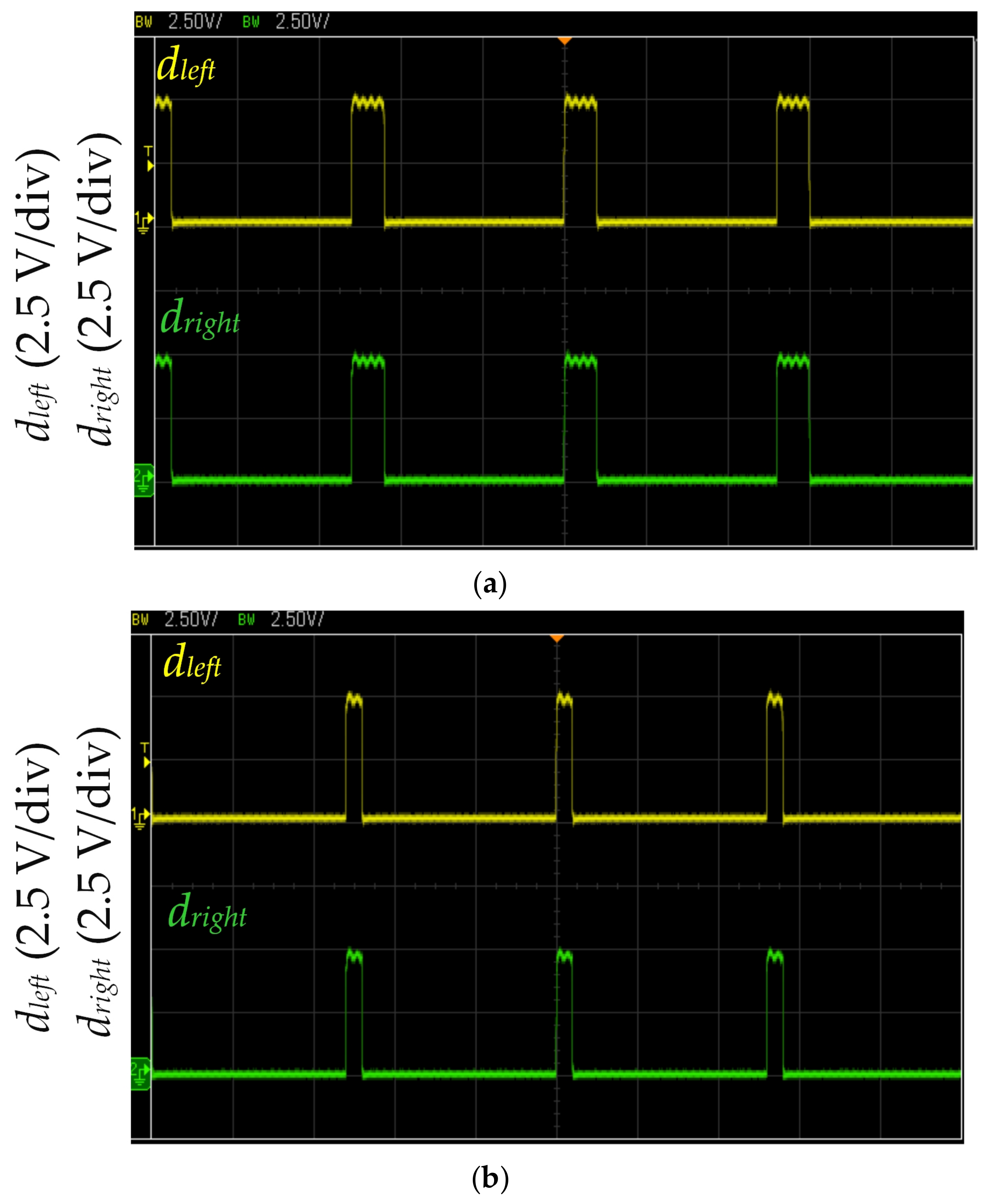
Figure 15 shows the measured MCU output dleft and dright waveforms when an obstacle is ahead of the self-driving electric mobile robot. dleft and dright drive the left and right motors, respectively. Figure 15a shows an obstacle 10 cm ahead identified by three infrared sensors. The proposed LCOT control strategy calculates dleft and dright according to Equation (7). When the operation time of the self-driving electric mobile robot is ΔT = 0.2 s, dleft and dright are 0.15 (frequency of 200 kHz). The proposed LCOT control strategy controls deceleration when an obstacle ahead is verified. As the proposed LCOT control strategy is based on the relationship between the logarithm curve and operation time, the deceleration of the self-driving electric mobile robot is mild and stable. Figure 15b shows an obstacle ahead being identified by three infrared sensors. The MCU duty cycles dleft and dright are 0.1 with a frequency of 200 kHz (as shown in Figure 10). Therefore, the self-driving electric mobile robot could stop instantly. This method could effectively avoid collision with the obstacle but might result in a strong vibration which could be uncomfortable for passengers.
Table 3 shows the characteristics comparison of the two methods. The self-driving electric mobile robot used the proposed LCOT control strategy for straight-line running, right turning, and left turning based on the relationship between the logarithm curve and operation time, where the acceleration is mild and stable. This proposed LCOT control strategy is better than the fixed duty cycle method because the fixed duty cycle method only maintains a constant speed, and the speed cannot be increased effectively. This leads to lower efficiency. Finally, when there is an obstacle ahead, the proposed LCOT control strategy can perform mild deceleration based on the relationship between the logarithm curve and operation time, reducing the impact on the self-driving electric mobile robot. On the contrary, the fixed duty cycle method stops the mobile robot immediately, resulting in a stronger vibration of the self-driving electric mobile robot.
Table 4 shows the performance comparison of the two methods. First, the mobile robot ran in the test path for ten loops with a total length of 3000 cm with no obstacles added. For the experiment of the straight-line and right-turn tests as shown in Figure 11b, the recorded operating time and speed of the self-driving electric mobile robot showed that the working time (300 s) and speed (10 cm/s) with the proposed LCOT control strategy were better than the time (450 s) and the speed (6.67 cm/s) with the fixed duty cycle method. Second, the mobile robot moved in the test path for ten loops with a total length of 3000 cm without obstacles. The test was for the straight line and left turns, as shown in Figure 11c. The recorded operating time and speed of the self-driving electric mobile robot indicated that the working time (301 s) and speed (10 cm/s) of the proposed LCOT control strategy were better than the time (451 s) and the speed (6.67 cm/s) of the fixed duty cycle method. Consequently, the experimental results verify the high efficiency, stability, and reliability of the proposed LCOT control strategy.
Table 4.
Performance comparison of the two methods.
5. Conclusions
This study proposed the LCOT control strategy based on the relationship between the logarithm curve and operation time for high efficiency, stability, and reliability while driving. The self-driving electric mobile robot performed straight running, left turning, right turning, and obstacle encountering. Based on the logarithm curve and operation time, the self-driving electric mobile robot performed mild and soft acceleration and deceleration on the path. This test measured and compared the proposed LCOT control strategy and fixed duty cycle method. The fixed duty cycle method for the self-driving electric mobile robot maintained a constant speed during straight running, turning left, and turning right, and the mobile robot was stopped immediately when an obstacle was encountered, leading to a strong vibration of the self-driving electric mobile robot, causing discomfort for the passengers. The proposed LCOT control strategy spent 300 s for running 3000 cm and a speed of 10 cm/s. However, the fixed duty cycle method spent 450 s running 3000 cm and a speed of 6.67 cm/s. The proposed LCOT control strategy had much better efficiency than the fixed duty cycle method. This novel LCOT control strategy was based on the relationship between the logarithm curve and operation time, and the system design was simple and easy to be implemented, with a reduced working load of the controller and better system efficiency. Consequently, the work efficiency of the self-driving electric mobile robot was increased effectively.
In the future, we will focus on the LCOT control strategy for the acceleration and deceleration of the self-driving electric mobile robot to reduce the vibration for upgrading the ride quality for the passengers. This novel LCOT control strategy can be applied to larger self-driving electric cars, such as karts and golf carts. This novel LCOT control strategy combined with image processing technology can be extended to drones and unmanned ships and tested in different fields to enhance the energy efficiency of unmanned vehicles.
Author Contributions
H.-D.L., G.-J.G., Y.-H.H. and S.-D.L. conceived of the presented idea designed and experimental; H.-D.L. and G.-J.G. performed testing and verification; H.-D.L., G.-J.G., Y.-H.H. and S.-D.L. wrote the original draft of this article; H.-D.L., G.-J.G., Y.-H.H. and S.-D.L. wrote the review and edited this article; S.-D.L. supervised the findings of this work; all authors provided critical feedback and helped shape the research, analysis, and manuscript. All authors have read and agreed to the published version of the manuscript.
Funding
This research was funded by the National Science and Technology Council, Taiwan, R.O.C., grant number MOST 111-2221-E-167-004. The authors also sincerely appreciate the considerable support from the National Taiwan Normal University Subsidy Policy to Enhance Academic Research Projects.
Data Availability Statement
Not applicable.
Acknowledgments
The authors also acknowledge the National Science and Technology Council, Taiwan, R.O.C., grant number MOST 111-2221-E-167-004, and sincerely appreciate the considerable support from the National Taiwan Normal University Subsidy Policy to Enhance Academic Research Projects.
Conflicts of Interest
The authors declare no conflict of interest.
References
- Li, S.E.; Guo, Q.; Xin, L.; Cheng, B.; Li, K. Fuel-Saving Servo-Loop Control for an Adaptive Cruise Control System of Road Vehicles with Step-Gear Transmission. IEEE Trans. Veh. Technol. 2017, 66, 2033–2043. [Google Scholar] [CrossRef]
- Tang, X.; Chen, J.; Yang, K.; Toyoda, M.; Liu, T.; Hu, X. Visual Detection and Deep Reinforcement Learning-Based Car following and Energy Management for Hybrid Electric Vehicles. IEEE Trans. Transp. Electrif. 2022, 8, 2501–2515. [Google Scholar] [CrossRef]
- Liu, B.; Ghosal, D.; Chuah, C.-N.; Zhang, H.M. Reducing Greenhouse Effects via Fuel Consumption-Aware Variable Speed Limit (FC-VSL). IEEE Trans. Veh. Technol. 2012, 61, 111–122. [Google Scholar] [CrossRef]
- Kanellos, F.D.; Grigoroudis, E.; Hope, C.; Kouikoglou, V.S.; Phillis, Y.A. Optimal GHG Emission Abatement and Aggregate Economic Damages of Global Warming. IEEE Syst. J. 2017, 11, 2784–2793. [Google Scholar] [CrossRef]
- Borenius, S.; Tuomainen, P.; Tompuri, J.; Mansikkamäki, J.; Lehtonen, M.; Hämmäinen, H.; Kantola, R. Scenarios on the Impact of Electric Vehicles on Distribution Grids. Energies 2022, 15, 4534. [Google Scholar] [CrossRef]
- Nikitenko, A.; Kostin, M.; Mishchenko, T.; Hoholyuk, O. Electrodynamics of Power Losses in the Devices of Inter-Substation Zones of AC Electric Traction Systems. Energies 2022, 15, 4552. [Google Scholar] [CrossRef]
- Li, M.; Wang, H.; Wang, H. Resilience Assessment and Optimization for Urban Rail Transit Networks: A Case Study of Beijing Subway Network. IEEE Access 2019, 7, 71221–71234. [Google Scholar] [CrossRef]
- Gkiotsalitis, K. Bus Holding of Electric Buses with Scheduled Charging Times. IEEE Trans. Intell. Transp. Syst. 2021, 22, 6760–6771. [Google Scholar] [CrossRef]
- Bruzinga, G.R.; Filho, A.J.S.; Pelizari, A. Analysis and Design of 3 kW Axial Flux Permanent Magnet Synchronous Motor for Electric Car. IEEE Lat. Am. Trans. 2022, 20, 855–863. [Google Scholar] [CrossRef]
- Yu, W.; Hua, W.; Qi, J.; Zhang, H.; Zhang, G.; Xiao, H.; Xu, S.; Ma, G. Coupled Magnetic Field-Thermal Network Analysis of Modular-Spoke-Type Permanent-Magnet Machine for Electric Motorcycle. IEEE Trans. Energy Convers. 2021, 36, 120–130. [Google Scholar] [CrossRef]
- Karnouskos, S. Self-Driving Car Acceptance and the Role of Ethics. IEEE Trans. Eng. Manag. 2020, 67, 252–265. [Google Scholar] [CrossRef]
- Chowdhury, A.; Karmakar, G.C.; Kamruzzaman, J.; Islam, S. Trustworthiness of Self-Driving Vehicles for Intelligent Transportation Systems in Industry Applications. IEEE Trans. Ind. Inform. 2020, 17, 961–970. [Google Scholar] [CrossRef]
- Tian, H.; Xu, X.; Qi, L.; Zhang, X.; Dou, W.; Yu, S.; Ni, Q. CoPace: Edge Computation Offloading and Caching for Self-Driving With Deep Reinforcement Learning. IEEE Trans. Veh. Technol. 2021, 70, 13281–13293. [Google Scholar] [CrossRef]
- Dzeparoska, K.; Beigi-Mohammadi, N.; Tizghadam, A.; Leon-Garcia, A. Towards a Self-Driving Management System for the Automated Realization of Intents. IEEE Access 2021, 9, 159882–159907. [Google Scholar] [CrossRef]
- Ni, J.; Shen, K.; Chen, Y.; Cao, W.; Yang, S.X. An Improved Deep Network-Based Scene Classification Method for Self-Driving Cars. IEEE Trans. Instrum. Meas. 2022, 71, 1–14. [Google Scholar] [CrossRef]
- Shi, Y.; Li, Y.; Fan, J.; Wang, T.; Yin, T. A Novel Network Architecture of Decision-Making for Self-Driving Vehicles Based on Long Short-Term Memory and Grasshopper Optimization Algorithm. IEEE Access 2020, 8, 155429–155440. [Google Scholar] [CrossRef]
- Park, J.-H.; Jo, W.; Jeon, E.-T.; Kim, S.-H.; Lee, C.-H.; Lee, J.-H.; Lee, J.-H.; Yi, J.; Won, C.-Y. Variable Switching Frequency Control-Based Six-Step Operation Method of a Traction Inverter for Driving an Interior Permanent Magnet Synchronous Motor for a Railroad Car. IEEE Access 2020, 10, 33829–33843. [Google Scholar] [CrossRef]
- Gupta, V.; Deb, A. Speed control of brushed DC motor for low cost electric cars. In Proceedings of the 2012 IEEE International Electric Vehicle Conference, Greenville, SC, USA, 4–8 March 2012; pp. 1–3. [Google Scholar] [CrossRef]
- Nowosielski, A.; Małecki, K.; Forczmanski, P.; Smolinski, A.; Krzywicki, K. Embedded Night-Vision System for Pedestrian Detection. IEEE Sens. J. 2020, 20, 9293–9304. [Google Scholar] [CrossRef]
- Kamalakkannan, S.; Hariharan, V.C.; Raghu, U. Three-Wheeled Autonomous E-Car. In Proceedings of the 2020 International Conference on System, Computation, Automation and Networking (ICSCAN), Pondicherry, India, 3–4 July 2020; pp. 1–5. [Google Scholar] [CrossRef]
- Zhang, W.; Zhang, B.; Li, S. A Wide-Stable-Region Logarithm-Type Slope Compensation for Peak-Current-Mode Controlled Boost Converter. IEEE Trans. Circuits Syst. II Express Briefs 2022, 69, 2927–2931. [Google Scholar] [CrossRef]
- Sviatov, K.; Yarushkina, N.; Kanin, D.; Rubtcov, I.; Jitkov, R.; Mikhailov, V.; Kanin, P. Functional Model of a Self-Driving Car Control System. Technologies 2021, 9, 100. [Google Scholar] [CrossRef]


Publisher’s Note: MDPI stays neutral with regard to jurisdictional claims in published maps and institutional affiliations. |
© 2022 by the authors. Licensee MDPI, Basel, Switzerland. This article is an open access article distributed under the terms and conditions of the Creative Commons Attribution (CC BY) license (https://creativecommons.org/licenses/by/4.0/).