Optimization of the Control of Electromagnetic Brakes in the Stand for Tuning Internal Combustion Engines Using ID Regulators of Fractional Order

Abstract

This work is aimed at developing a stand for tuning the fuel system of an internal combustion engine based on two electromagnetic retarders connected to the driving wheels of a car to simulate a load, and a microprocessor-based torque control system for each brake. In accordance with the terms of reference from the specialists of the automotive service center, such a stand should provide two main modes of operation: (1) stabilization of the speed of the drive wheels in the entire range of loads (fuel supply); (2) engine acceleration and deceleration according to linear tachograms in the range from minimum to maximum speed to determine the dependence of engine power and torque on speed. The purpose of this research is the synthesis of controllers, testing, the choice of the structural scheme, and the parameters of the control and data processing system in the stand for the precision tuning of internal combustion engines. Based on a preliminary analysis of the system, taking into account the mechanical connection of the wheels through the main gear and the car differential, the nonlinear dependence of the electromagnetic torque on the current and retarder speed, and subsequent experimental results, we obtained two types of controller—a third-order aperiodic transfer function and a fractional aperiodic transfer function of order 1.6. This made it possible to synthesize a family of controllers that ensure the operation of the stand in the required modes: synchronization of wheel speeds during engine acceleration; stabilization of the reference speed when the engine torque is changed from minimum to maximum due to fuel supply; measurement of the maximum power and torque of the internal combustion engine during the formation of a triangular tachogram with a given acceleration to compensate for the dynamic component of the torque due to mechanical inertia. The system with the PID controller configured in MATLAB in the “Tune” package has the best performance, but the smallest overshoot and the best dynamic accuracy are ensured by the PIDI^γI^µ fractional–integral controller, where the system is characterized by a fractional order of astaticism 1.6. Such a controller for each electromagnetic retarder serves as the basis of the microprocessor-based control, data acquisition, processing, graphical display system, and will also be used to develop a similar bench for tuning four-wheel-drive vehicles.

1. Introduction: Fractional Calculus in Control Systems

The first historical mention associated with fractional calculus was recorded over three centuries ago. In letters between Guillaume François L’Hopital and Gottfried Wilhelm Leibniz, the possibility of an order of differentiation not of an integer but of an intermediate value, equal to 1/2, was described [1]. In 1738, L. Euler noticed that the calculation of the derivative $\frac{d^{\beta }y}{d{x}^{\beta }}$ of a power function $y=x^m$ could be performed with a fractional value $\beta$. Less than 100 years later, in 1819, a publication by S. Lacroix appeared, where Euler’s idea was repeated, and an explicit formula for calculating the derivative of a power function using the gamma function $\mathsf{\Gamma }\left(x\right)$ was given, generalizing the factorial function to the case of a non-integer argument. In 1822, J. Fourier derived a formula for calculating the fractional derivative for any function [2]. He obtained it by integrating by parts the inverse transformation formula. Some of the first and most complete research in this branch of mathematics was carried out by J. Liouville in 1832–1837. Although further research significantly developed and modified his ideas, the definition of a fractional differential formulated by Liouville laid the foundation and made it possible to expand the scope of fractional calculus in geometry, physics, and mechanics [3]:

$$D^{\gamma }{x}^{-\alpha }=\frac{{\left(-1\right)}^{\gamma }\mathsf{\Gamma }\left(\alpha +\gamma \right)}{\mathsf{\Gamma }\left(\alpha \right)}{x}^{-\alpha -\gamma }.$$

(1)

B. Riemann in 1847 applied the Taylor series expansion and the definite integral to series with non-integer order [4,5] for fractional integration, but the additional function $\mathsf{\Psi }\left(x\right)$ caused some problems. However, after the work of N. Ya. Sonin [6], A. V. Letnikov [7], and H. Laurent [8], this problem was solved. The formulated concept of a fractional integral and a fractional derivative were given the name Riemann–Liouville, in honor of the authors of the idea:

$$D^{-\gamma }f\left(x\right)=\frac{1}{\mathsf{\Gamma }\left(\gamma \right)}{\displaystyle \underset{c}{\overset{x}{\int }}{\left(x-t\right)}^{\gamma -1}f\left(t\right)dt}.$$

(2)

Almost simultaneously, Grunwald [9] and Letnikov [7], having decided to get rid of the restrictions in the Liouville formulas, derived the fractional differential formula as the boundary of the difference relation ${\mathsf{\Delta }}_{\mathsf{\Delta }t}^{\gamma }f/\mathsf{\Delta }{t}^{\gamma }$:

$$D^{\gamma }f\left(x\right)=\underset{\mathsf{\Delta }t\to 0}{\lim }\frac{{\displaystyle \sum _{k=0}^{\infty }{\left(-1\right)}^k\left(\begin{array}{l}\gamma \\ k\end{array}\right)f\left(x-k\mathsf{\Delta }t\right)}}{\mathsf{\Delta }{t}^{\gamma }},$$

(3)

where $\left(\begin{array}{l}\gamma \\ k\end{array}\right)$ are generalized binomial coefficients.

Expression (3) is now called the Grunwald–Letnikov form.

We should also mention the works of A. Heaviside [10], who used operational calculus to solve certain problems in electromagnetic theory. G. Weyl [11] in 1917 defined fractional integration for periodic functions; A. Marcho [12] in 1927 developed an integral version of the form of the Grunwal–Letnikov fractional derivative; M. Caputo [13] reformulated the definitions of the Riemann–Liouville fractional derivative to use more “classical” initial values.

The mathematical applications of integrals and derivatives with fractional degrees expanded so much in the second half of the 20th century that in 1974, the first conference devoted to fractional calculus was held in New Haven [14]. In the same year, the first book by Oldham and Spagnier [15] was published. Several significant works by Miller and Ross, Samko [16], and Podlubny appeared. In 1998, the first issue of the mathematical journal “Fractional Calculus and Applied Analysis” was published. In 2004, a large conference “Fractional differentiation and its applications” was held in Bordeaux with 104 reports related to the solution of various scientific and engineering problems using this mathematical apparatus: inverse mechanical problems; stochastic kinetics and dynamic chaos; movement in a viscous fluid; distribution of heat flow; electrochemistry of electrodes; dynamics of a turbulent medium; filtration in a porous medium; rheology of viscoelastic materials; electrical engineering and radio engineering; plasma physics; quantum optics and nanophysics; laser cooling of atoms; astrophysics and cosmology; biophysics and medicine. The presence of a fractional time derivative is interpreted as a special property of this process, called memory or heredity [17]. Fractional derivatives with coordinates reflect a medium with inhomogeneities of a special kind, referred to as being self-similar, or as fractals. Such structures are found in turbulent flows, plasma, and interstellar media. In 1991, S. Westerlund suggested using fractional derivatives to describe the process of propagation of plane electromagnetic waves in an isotropic homogeneous dielectric medium with losses, in the generalized form of the equations of Maxwell, Newton and Hooke, in Einstein’s theory of relativity [18]. It was shown in [19] that fractional derivatives make it possible to describe better the physical processes of the working fluid in a hydrostatic drive.

Areas of application of fractional calculus in automatic control can be divided into two groups [20]. The first one is formed by methods of mathematical and computer modeling of fractional order systems. The second group includes methods of using fractional calculus for the synthesis of control systems for dynamic systems of both integer and fractional orders, in particular, the synthesis of controllers of non-integer order, the structure of which is similar to a PID controller [21]. The use of a differential and an integral with a fractional order makes it possible to obtain a more flexible controller in tuning, which is denoted $P{I}^{\gamma }{D}^{\mu }$ and is described by the following transfer function [22,23,24]:

$$\begin{array}{l}{D}^{\gamma }f\left(x\right)=\underset{\mathsf{\Delta }t\to 0}{\lim }\frac{{\displaystyle \sum _{k=0}^{\infty }{\left(-1\right)}^k\left(\begin{array}{l}\gamma \\ k\end{array}\right)f\left(x-k\mathsf{\Delta }t\right)}}{\mathsf{\Delta }{t}^{\gamma }},\\ G(s)=\frac{U(s)}{E(s)}=K_P+{\left(T_{I}s\right)}^{-\gamma }+{\left(T_{D}s\right)}^{\mu }.\end{array}$$

(4)

Such a $P{I}^{\gamma }{D}^{\mu }$ controller is formally an infinite-order filter [25]. Additionally, in the theory of automatic control, other types of fractional-order controllers have been used—the TID controller [26], the CRONE controller from the French abbreviation “Contrôle robuste des commandes non entières” [27], and the fractional lead–lag compensator [28,29]—in an attempt to achieve “fractal robustness”. However, there is no specific methodology for calculating the parameters of a $P{I}^{\gamma }{D}^{\mu }$ controller, in contrast to the traditional PID.

For the $P{I}^{\gamma }{D}^{\mu }$ controller, you can select five values, three of which are coefficients, and two of which are fractional orders of the derivative and integral. However, such freedom of choice comes at a price—a complicated search for the controller parameters for a transient with the desired quality. One can use the pole distribution scheme of the characteristic equation in the complex plane, and one can use such optimization procedures as genetic algorithms, the particle swarm method, etc.

One of the methods to simplify the search for the necessary structure and parameters of the regulator is a correction in accordance with the principles of subordinate regulation. The most common settings are with an astatic order of 1 $W_{op.}^1(s)$ and 2 $W_{op.}^2(s)$:

$$\begin{array}{l}{D}^{\gamma }f\left(x\right)=\underset{\mathsf{\Delta }t\to 0}{\lim }{W}_{op}^1\left(s\right)=\frac{1}{2T_{v}s\left(T_{\nu }s+1\right)},\\ W_{op}^2\left(s\right)=\frac{4T_{\nu }s+1}{8T_v^2{s}^2\left(T_{\nu }s+1\right)}.\end{array}$$

(5)

where $T_v$ is the small uncompensated time constant of the control object.

Fractional calculus makes it possible to expand the value of the non-integer astatic order with the corresponding transfer functions:

$$W_{op}^{\mu }\left(s\right)=\frac{1}{a{T}_{\nu }^{\mu }{s}^{\mu }\cdot (T_{\nu }s+1)}, 0<\mu <1,$$

(6)

$$W_{op}^{1+\mu }\left(s\right)=\frac{1}{a{T}_v^{\mu -1}{s}^{\mu -1}}\frac{b{T}_{v}s+1}{b{T}_{v}s}\frac{1}{(T_{v}s+1)}, 1<\mu <2,$$

(7)

where $a, b$ are the system setting parameters.

For the synthesis of systems with the maximum possible speed and a given allowable overshoot when a single jump is applied to the input, an additional criterion for assessing the quality of the system can be formulated in the following form:

$$F={\displaystyle \sum _{i=1}^N\{\begin{array}{l}{\left(1-Y_i\right)}_{}\forall Y_i<1\\ {\left(\frac{1}{\delta }\left(1-Y_i\right)\right)}^2 \forall Y_i>1\end{array}\to Min},$$

(8)

where $\delta$ is the allowable overshoot.

This criterion can be used when searching for controller parameters, since for a system with Transfer Function (6), the function $F\left(a{,}_{}\mu {,}_{}\delta \right)$ is characterized by the presence of an extremum (Figure 1a), which is absent when using the traditional criterion of minimum mean square error. Processing the results for $\delta =0.05$, which satisfies the requirements of most technical systems, makes it possible to obtain a calculated empirical dependence $a\left(\mu \right)$, on the basis of which the choice of optimal contour parameters is simplified:

$$a\approx \frac{\mu }{4.683-5.897\mu +1.595{\mu }^2}{,}_{}0.5\le \mu \le 0.9.$$

(9)

For systems with astatic order from 1 to 2 with Transfer Function (7), the dependence $F\left(a{,}_{}b{,}_{}\mu {,}_{}\delta \right)$ is also characterized by the presence of an extremum (Figure 1b). For $\delta =0.05$ the following calculation expressions are obtained:

$$\{\begin{array}{l}a\approx \exp \left(-10.27+7.831\mu \right)\\ b\approx 7.336+0.792a+3.83\ln (a)\end{array} \forall 1.3\le \mu \le 1.9.$$

(10)

After choosing the optimal transfer function of the open loop $W_{op}\left(s\right)$, the transfer function of the controller $W_{reg}\left(s\right)$ is determined from the relation $W_{reg}\left(s\right)=\frac{W_{op}\left(s\right)}{W_{obj}\left(s\right)}$. THis can consist of fractional integral, differential, or aperiodic links, depending on the mathematical model of the object $W_{obj}\left(s\right)$, which can also include blocks with fractional and integer order. Accordingly, the following pairs may arise:

• Integer controller–integer control object;
• Controller with fractional order–integer control object;
• Integer controller–control object with a fractional order;
• Controller with fractional order–control object with fractional order.

The next task is the technical implementation of the obtained regulators. From a theoretical point of view, an operator $s^{\mu }$ with a fractional order $\mu$ turns into a transfer function with an infinite integer order, which leads to an infinite number of terms in the Riemann–Liouville and Grunwal–Letnikov forms. In practice, approximate solutions are used in the selected frequency range, which can be divided according to the type of implementation into analog ones with various R–L–C combinations and discrete ones for calculation in microcontrollers [30,31,32].

Among the most popular are methods that use indirect discretization with the recursive approximation algorithm of Ostaloup [33], Carlson [34], direct power series expansion of the Euler operator [35], continuous fraction expansion (CFE) [36,37,38], a filter with a finite impulse response (FIR filter) [39], the B-spline function [40], the Podlubny matrix approach [41], and the discrete Grunwal–Letnikov operator model [42].

Based on the Riemann–Liouville form, it is possible to introduce a corrective bias in the denominator, which reduces the regular error by dozens of times without applying corrective calculations [43]. As a result, we get:

$$I_{t_i}^{\mu }f\left(t\right)=\frac{\mathsf{\Delta }{t}^{\mu }}{\mathsf{\Gamma }\left(1+\mu \right)}{\displaystyle \sum _{j=1}^i\left(j^{\mu }-{\left(j-1\right)}^{\mu }\right)f_{i-j+1}}=\frac{\mathsf{\Delta }{t}^{\mu }}{\mathsf{\Gamma }\left(1+\mu \right)}{\displaystyle \sum _{j=1}^i{k}_j{f}_{i-j+1}}.$$

(11)

It is important that $k_j=\left(j^{\mu }-{\left(j-1\right)}^{\mu }\right)$ are an array of constants that are calculated in advance, which simplifies the task of the microcontroller. However, at each quantization period, it is necessary to calculate the sum of pairwise products of the coefficients $k_j$ and previous values of the input signal $f_{i-j+1}$, which takes the time of the controller and requires the storage of vectors of constants and the history of the signal change. The maximum number of row members is determined by the amount of RAM. The required array size for calculation with a permissible relative error ε is determined by the expression $N={\left(\frac{1}{\epsilon }\frac{\mathsf{\Gamma }\left(1+\mu \right)}{\mathsf{\Gamma }\left(\mu \right)\mathsf{\Delta }{t}^{\mu }}\right)}^{\frac{1}{\mu }}$. For example, for µ = 0.5 and ε = 0.05, 315 points must be stored, and to ensure $\epsilon =0.02$, this figure is already 1964. Storage of such a volume of data exceeds the capabilities of many single-chip processors.

Analysis of the coefficients in Equation (11), when constructing graphs in logarithmic axes, shows that, starting from the 50th, …, 100th term, the coefficients lie almost on straight lines, which corresponds to a geometric progression with an error of a fraction of a percent. This makes it possible to significantly simplify the procedure for calculating the fractional integral and reduce it to several tens or hundreds of combinations of multiplication and addition operations during one quantization period. The most important thing is that only a limited number of input signal values and the same number of coefficients must be stored in the processor memory [43]. To optimize calculations, it is advisable to store the last values of the input signal in an organized ring array with numbering from 0 to $n_{\dim }-1$. If you specify $n_{\dim }=2^k$ and choose k from 6 to 8, reserving arrays of 64, 128 or 256 elements, then the procedure for changing the number j of the element of the ring array is described by a simple expression $j=\left(j+1\right)\&mask,$ where $mask=\left(n_{\dim }-1\right)=0b\mathrm{0...11}$ is a binary number in which the k least significant digits are equal to 1. The algorithm for calculating the fractional integral is provided in Figure 2, where in loop 2, the exact value of the fractional integral over the $n_{\dim }-1$ last points is calculated, and in loop 1, the component calculated from the old values of the input coordinate as the sum of a geometric progression is added to this value.

Such an algorithm for the approximate calculation of fractional integrals reduces the required amount of memory for storing arrays of coefficients and the history of the input signal by hundreds to thousands of times and reduces the processor time required to calculate the controller signal by the same factor. This allows, on the basis of modern microcontrollers, such as Intel^®Quark™ SoC X1000, STM32F4, FPGA Altera Cyclone V, the implementation of fractional integral–differential controllers with high speed.

2. Fractional Order Regulators in the Control System of Electromagnetic Brakes in the Stand for Tuning of Internal Combustion Engines

The presented theoretical information was used in the development of an electromagnetic brake control system in a stand for precision tuning of the fuel system of internal combustion engines (ICE) of sports cars. The principle of operation of an inductive brake (Figure 3) is based on the dissipation of mechanical rotational energy into heat due to the generation of eddy currents that occur in a massive metal conductor when it moves in a magnetic field created by coils. An inductive brake consists of a stator and a pair of rotors rigidly connected to each other. The stator is made of a special conductive material and acts as an inductor. It consists of electromagnets connected in series. The interaction of the magnetic field and eddy currents creates a moment [44], which tends to stop the rotor, while heating it. Excess heat is removed by the airflow created by the blades on the disks.

Inductive brakes (Figure 3) are widely used in freight and passenger transport, industry (wind generators, lifts), and emergency braking systems, as well as in test stands [45].

Two TELMA retarders are used in the developed stand for tuning sports cars of various classes participating in international rallies. They are installed instead of drive wheels and allow for the entire range of speed and torque of the internal combustion engine, adjusting the ignition timing and fuel mixture composition so as to provide maximum torque and minimum fuel consumption (Figure 4) [46,47]. Compared to the most common drum (roller) type stands, on which a car is mounted attached to the wall with cables, the advantage of such a stand is the independence of the wheels, the absence of vibrations due to spikes on the drums or wheels, and incomparably greater safety, since the car remains stationary, cannot move from the drums, cannot jump and fall off the cables, which is especially dangerous at high loads and high wheel speeds.

However, the control system built by the masters of the center turned out to be ineffective. Synchronization took a long time (tens of seconds), and minor changes in the torque and speed of the internal combustion engine led to oscillations.

In this regard, the task arose of studying the system and synthesizing regulators that would provide fast (no more than 1–3 s) synchronization of the wheel speed and fast transitions from one operating point to another.

Figure 5 shows a functional diagram of the stand for measuring the power and torque of an internal combustion engine, where P_e, T_e, ω_e are the power, torque and angular velocity of the internal combustion engine; T_EL, T_ER, ω_L, ω_R are torques and angular velocities of the left and right wheels (differential axle shafts), T_bL, T_bR are braking torques from the left and right retarders; ω_ref is speed reference signal; U_{PWM_L}, U_{PWM_R} are duty cycle of the PWM voltage of the left and right retarders. When the angle of inclination of the car’s gas pedal is increased, a certain amount of fuel is injected into the internal combustion engine, while the created mechanical energy is transferred through the transmission and differential to the wheels of the car, which begin to develop a certain speed. To tune the internal combustion engine, it is necessary to stabilize this speed at a given level at the maximum angle of inclination of the gas pedal, that is, at the maximum engine power. This is achieved thanks to the braking torque of the retarders, the value of which is regulated by the control system.

For preliminary study, a model of the control system and the mechanical part of the stand was developed, in which the following assumptions were made:

• Elastic connections and losses in the clutch, gearbox and cardan shaft are combined into one element;
• Power losses and elastic connections in the differential are not taken into account.

With these assumptions, the transfer of the power from the motor shaft to the symmetrical differential is described by the system of equations [48,49]:

$$\{\begin{array}{l}\frac{d{\omega }_L}{dt}{J}_L=T_L-T_{bL}+\mu T_d,\\ \frac{d{\omega }_R}{dt}{J}_R=T_R-T_{bR}-\mu T_d,\\ \frac{T_d}{2}=T_L=T_R,\\ \frac{d{T}_{ru}}{dt}{c}_u={\omega }_h-{\omega }_L-{\omega }_R,\\ T_{rv}=b_v\left({\omega }_h-{\omega }_L-{\omega }_R\right),\\ T_d=T_{ru}+T_{rv}.\end{array}$$

(12)

where J_L, J_R, ω_L, ω_R, T_L, T_R, T_bL, T_bR are the moments of inertia, angular velocity, torque and drag of the left and right wheels; μ_tr is the load asymmetry factor; T_rv is the torque of viscous friction of the cardan shaft; T_ru is the torque of elasticity of the chain from the engine to the differential; T_d is the torque that is transmitted by the differential to the axle; C_u, b_v are the coefficients of elastic bonds and viscous friction.

Since the axles of the driving wheels are not connected in any way, they can rotate at different speeds. This asymmetry is given in the model by a constant value ±μT_d in the system of Equation (12), although this value and sign may change during the real operation of the differential.

The braking torques are controlled by a system that consists of two subsystems for the left and right brakes. At the preliminary stage, models of various speed stabilization systems in each channel for the left and right axes were compared—a single-loop system with a PI-speed controller and a double-loop system with a PI-speed controller and a relay current or torque controller. In the models of the speed sensors, quantization with respect to time and in level is taken into account, and the induction brake coil is approximated by an aperiodic block with a non-linear dependence:

$$W_c(s)=\frac{i_b}{U}=\frac{1}{0.1s+1}, T_b=T_{\max }\sin \left(\frac{\pi }{2}\frac{i_b}{i_{\max }}\right)\frac{{\omega }_b}{{\omega }_{\max }},$$

(13)

where $T_{\max }$ is the maximum brake torque; $i_b$ is the instantaneous value of the current; ${\omega }_b$ is the angular velocity of the brake.

The system must operate in two modes.

In the calibration mode, the operator accelerates the internal combustion engine, but the speed of rotation of the wheels should be approximately the same. To do this, a command signal ${\omega }_{ref}$ is generated in the control system for each wheel, as the sum of the arithmetic mean instantaneous speed values and some lead Δ:

$${\omega }_{ref}=\frac{{\omega }_L+{\omega }_R}{2}+\mathsf{\Delta }.$$

(14)

The lead is reset to zero when switching to the speed stabilization mode, and ω_ref is equal to the value set by the operator. In this mode, the angular speeds of the wheels must be maintained constant regardless of the angle of the carburetor throttle, that is, the engine power. The simulation results showed that in all modes a two-loop system provides a better quality of the transient process than a single-loop one. However, in both cases, satisfactory results were obtained from the point of view of the problem posed [50]. Therefore, the final decision on the structure of the regulators was made only after testing the control system.

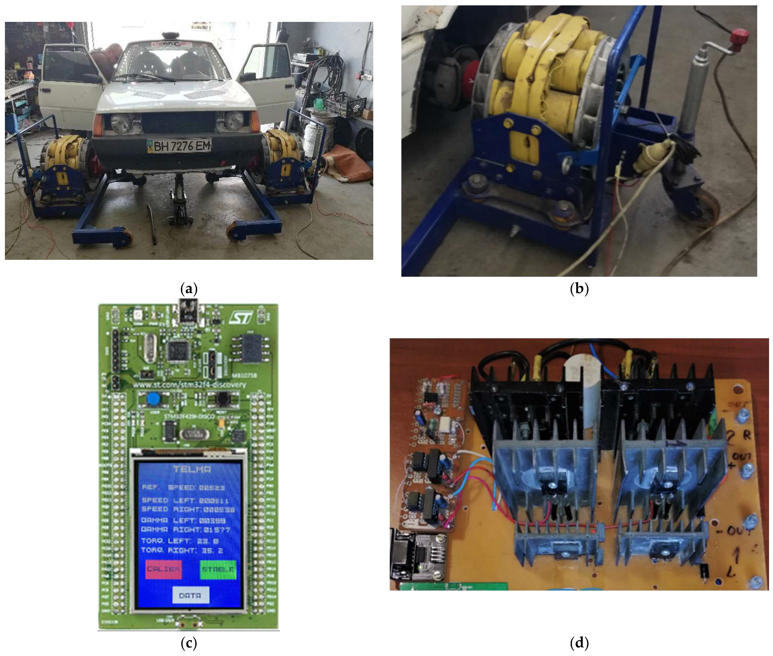
3. Experimental Studies for a Stand with Two Electromagnetic Retarders

The tests were carried out with a GT car with a nominal engine power of 90 hp. The left and right wheels of the machine are removed and induction brakes on special frames are attached directly to the axles (Figure 6).

The current regulation in the electromagnetic brake is carried out by means of a DC voltage PWM in a single-key inverter. G4PH40UD series IGBT is used as a power switch. A 30EPH06 series flyback diode is selected for overvoltage protection. The KBPC5010 diode bridge with a capacitive filter rectifies the voltage from a single-phase network and supplies a constant voltage to the transistors. Control signals are fed to the base through galvanic isolation—HCPL3120 optocouplers. Optocouplers are powered by DC/DC converter TMA1515D. The input of the optocouplers receives signals from the ports of the microcontroller 32F429IDISCOVERY (STM32F429ZI). The clock frequency of the microcontroller is 168 MHz. The frequency of pulse-width modulation—4 kHz—is provided by setting the counter AutoReload Register ARR = 41,999, which makes it possible to change the duty cycle from 0 to 41,999. For the speed loop, the sampling period is set to 10 ms.

The measurement of the torque of each electromagnetic brake is carried out using electronic scales XK3118T1, the load sensor of which is installed in the retarder case; the polling period is 100 ms.

To measure the rotation speed of the axes, OMRON E6B2-CWZ6C encoders with 2500 pulses per revolution are used. We obtain 10,000 pulses per revolution by setting the timers of the quadrature decoder with the determination of the leading and trailing edges of the pulse. The encoders are fixed on the frames and connected to the retarder axles by short belt drives, which protects the encoders from destruction due to vibration of the retarder axle.

For the first tests, a program was developed to interact with a 2.4 QVGA TFT display (Figure 6c), which displays “REF. SPEEED”, “SPEED LEFT” and “SPEED RIGHT”—the reference and current speeds of the left and right axes (in pulses for 10 ms); “GAMMA LEFT” and “GAMMA RIGHT”—duty cycles of the PWM voltage of the left and right induction brakes; and “TORQ. LEFT” and “TORQ. RIGHT”—left and right axle torque (kg m). The buttons “CALIBRE” and “STABLE” set calibration and stabilization modes, and the “DATA” button starts data transfer via USB to the terminal program “RealTerm: Serial Capture Program 3.0.1.44” with the formation of a text file of the “.csv” format.

This interface has limited functionality (the screen is small, graphs are built manually on a computer, data in the form of numbers are not very clear, two operators are needed—one is driving, and the second works with the controller). Therefore, after adjusting the regulators, a program was developed in the Java programming language to connect the controller to a computer via an Ethernet network. The interface of the created program is shown in Figure 7.

This interface makes it possible to display on the “speedometers” the measured speeds of the engine and wheels, the torques on the wheels, and the torque and power of the engine (without taking into account losses in the transmission). The screen also displays oscillograms of four parameters: speed, speed, torque, and power of the internal combustion engine. In another window, the results of data processing are displayed: graphs and tables of dependences of torque and power on speed, extreme values found by the program.

4. Identification of the Parameters of the Control Object Based on Preliminary Experimental Studies

Taking into account the obtained theoretical results, the greatest hopes were placed on a two-loop system with subordinate regulation. However, experimental studies showed that significant current ripples at the selected PWM frequency do not allow the implementation of relay controllers with the required trajectory processing accuracy, and torque sensors with 100 ms time quantization are also not able to meet the requirements for the test stand. In the general case, antiphase oscillations occurred, and with some regulator parameters, self-oscillations occurred with increasing power. The best results obtained—regulation time in the range from 3.3 to 4.1 s with an overshoot from 32.2% to 71.1%—do not satisfy the requirements for the system.

In a single-loop system with PID controllers for each semi-axis, despite significant overshoot and oscillation in the speed stabilization mode, after several attempts, it was possible to select the coefficients K_p = 50, K_i = 50, K_d = 9, at which values the obtained transient processes made it possible to identify the object parameters for several types of transfer functions:

$$W_{co1}\left(s\right)=\frac{K}{\left(a_{1}s+1\right)\left(a_{2}s+1\right)\left(a_{3}s+1\right)},$$

(15)

$$W_{co2}\left(s\right)=\frac{K}{\left(a_{1}s+1\right)\left(a_{2}s+1\right)},$$

(16)

$$W_{co3}\left(s\right)=\frac{K}{\left(a_{1}s+1\right)\left(a_{2}s+1\right)s},$$

(17)

$$W_{co4}\left(s\right)=\frac{K}{a_1{s}^{1+{\mu }_{co}}+a_2{s}^{{\mu }_{co}}+1}.$$

(18)

The graphs of the transient processes obtained as a result of the experiments made it possible to determine the unknown parameters in the Transfer Functions (15)–(18). A genetic algorithm was used, in which the tournament method was chosen for selection. New individuals inherited the genes of their parents by uniform crossing, the probability of mutation in the chromosome is 20%. The standard error F served as an estimate of the fitness of an individual.

The results of identification of the parameters transfer functions W_co1, W_co2, W_co3 and W_co4 are summarized in

Table 1. Results of identification of the control object.

Parameter	Transfer Function of the Control Object
	Wco1	Wco2	Wco3	Wco4
K	0.03729	0.06666	0.04069	0.11514
a1	0.7445	1.2856	0.2042	2.8951
a2	0.3208	0.8804	0.04813	1.8987
a3	0.7252	–	–	–
µco	–	–	–	0.6261
F	0.0130	0.0142	0.0275	0.0132

; the corresponding graphs of the experimental and calculated transient processes are compared in Figure 8.

Obviously, the models with transfer functions W_co1 and W_co4 are characterized by the smallest root mean square error. This allows them to be used as models of the control object.

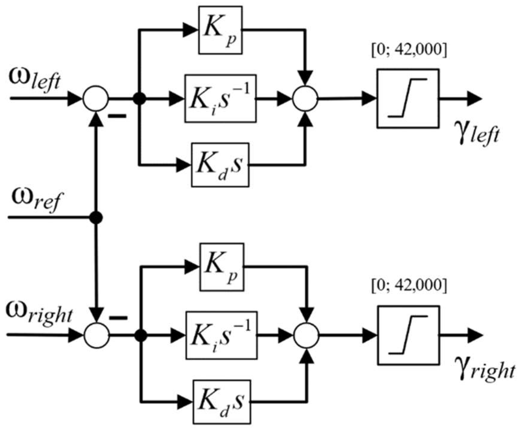
5. Synthesis of an Optimal Control System for Electromagnetic Retarders

The obtained identification results made it possible to significantly simplify the control system—to abandon the internal circuit and the compensator of antiphase oscillations. An independent regulator controls each of the two axes. Figure 9 shows a block diagram for a variant with classic PID controllers, where ω_ref, ω_left, ω_right are the reference signal and the speed of the left and right axes, respectively, and γ_left, γ_right are the PWM duty cycles of the power transistors.

Based on the obtained functions, the synthesis of three types of controllers was performed.

• For the Wco1 function in the “PID Controller” block of MATLAB Simulink, using the “Tune” procedure, the parameters of the classical PID controller were found, which turned out to be quite close to those found empirically: K_p = 65, K_i = 50, K_d = 15.
• Based on the Wco4 fractional order model, the circuit is tuned to a modular optimum with an equivalent transfer function:

$$W_{op.s}\left(s\right)=\frac{1}{2T_{f}s\left(T_{f}s+1\right)}=W_{sr}\left(s\right)\frac{1}{\left(T_{f}s+1\right)}\frac{K}{\left(a_1{s}^{1+{\mu }_{co}}+a_2{s}^{{\mu }_{co}}+1\right)},$$

(19)

where $T_f=0.05 s$ is the inertia of the first-order filter connected in the circuit of the differentiating component, taken as an uncompensated small time constant. Then, we obtain a D^γI^µI controller:

$$W_{sr}(s)=K_{1}s{s}^{{\mu }_{co}-1}+K_2{s}^{{\mu }_{co}-1}+K_3{s}^{-1},$$

(20)

where $K_1=\frac{a_1}{2T_{f}K}$, $K_2=\frac{a_2}{2T_{f}K}$, $K_3=\frac{1}{2T_{f}K}$.

3.

Additionally, on the basis of the fractional order model W_co4, taking into account (10), a controller is synthesized that ensures the astatism of the closed loop of the fractional order µ = 1 + µ_co. From the relation

$$W_{op.s}\left(s\right)=\frac{1}{a{T}_f^{\mu -1}{s}^{\mu -1}}\frac{b{T}_{f}s+1}{b{T}_{f}s}\frac{1}{\left(T_{f}s+1\right)}=W_{sr}\left(s\right)\frac{1}{\left(T_{f}s+1\right)}\frac{K}{\left(a_0{s}^{1+{\mu }_{co}}+a_1{s}^{{\mu }_{co}}+1\right)},$$

(21)

we obtain the transfer function of the controller from five components:

$$W_{sr}(s)=\frac{K_0}{s^{\mu -1}}\times \left(K_1{s}^{{\mu }_{co}+1}+K_2{s}^{{\mu }_{co}}+K_3{s}^{{\mu }_{co}-1}+\frac{K_4}{s}+K_5\right).$$

(22)

where $K_0=\frac{1}{a{T}_f^{\mu -1}}$, $K_1=\frac{a_1}{k_{f}K}$, $K_2=\frac{a_{2}b{T}_f+a_1}{b{T}_{f}K}$, $K_3=\frac{a_2}{b{T}_{f}K}$, $K_4=\frac{1}{b{T}_{f}K}$, $K_5=\frac{1}{K}$.

For µ = 1 + µ_co, the controller consists of traditional PID and fractional–integral components with orders 1 + µ_co and µ_co:

$$W_{sr}(s)=K_0{K}_{1}s+K_0{K}_2+\frac{K_0{K}_3}{s}+\frac{K_0{K}_4}{s^{1+{\mu }_{co}}}+\frac{K_0{K}_5}{s^{{\mu }_{co}}}.$$

(23)

It should be noted that similar controllers have also been obtained for several other electrical control objects [51,52].

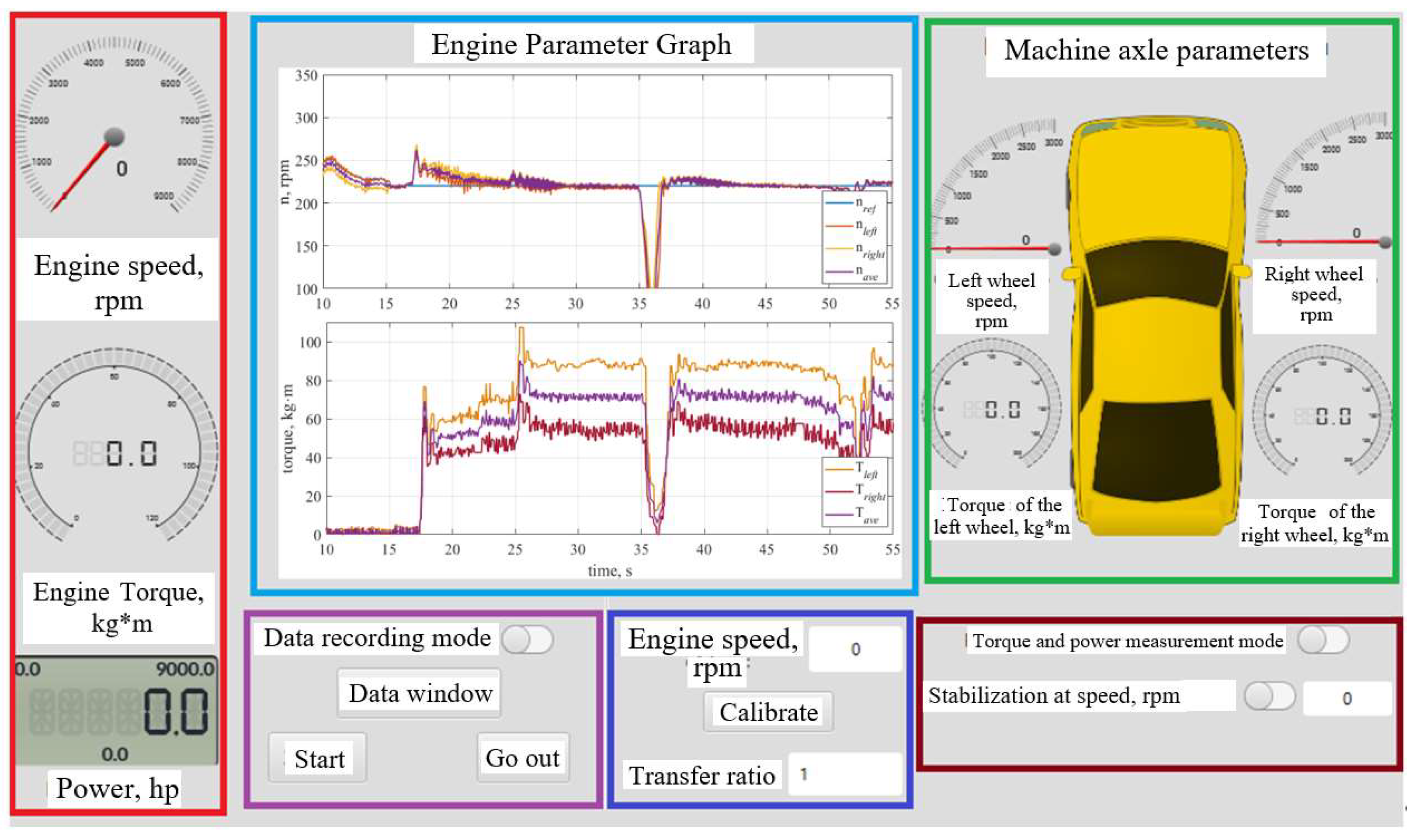
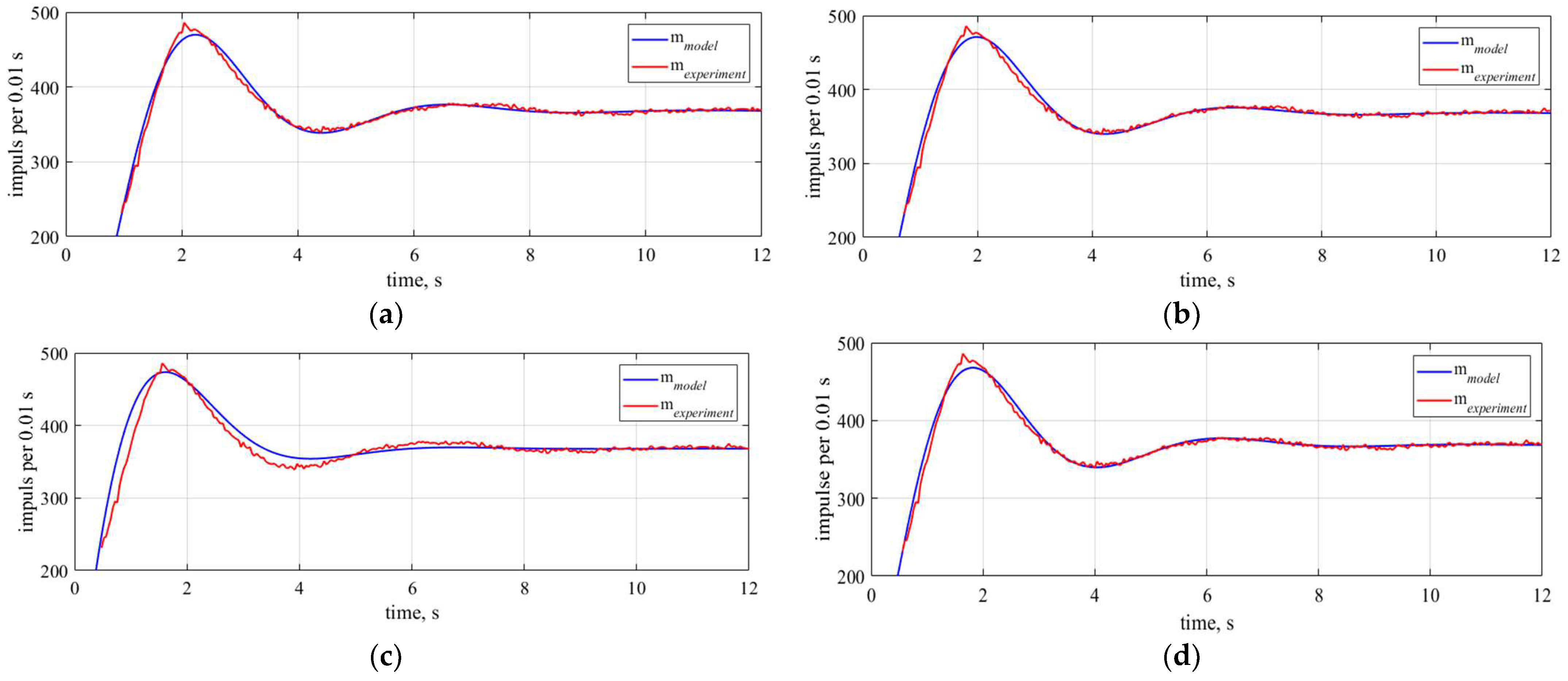
6. Experimental Studies of the Tuned Stand and Discussion of the Results

After programming the system with the developed regulators, transient graphs were obtained, which are shown in Figure 10. Transitions from the calibration mode to the stabilization mode (for 10–15 s) and the reaction to an increase in fuel supply after a short-term decrease in speed (for 35–45 s) were studied.

Areas of rapid increase in the fuel supply to the internal combustion engine in the speed stabilization mode were selected from the obtained graphs and combined in time (Figure 11).

These plots compare performance (as lane entry time ±2% of speed setpoint) and overshoot.

The PID controller provides the best performance (2.55 s), but with the highest overshoot δ₁ = 27.6%. With the DγIµI controller, the overshoot was δ₂ = 16.3%, and the duration of the transient process was 4.42 s. The smallest overshoot was obtained with a PIDI^γI^µ controller—δ₃ = 3.3% with a formal duration of the transient process of 3.8 s, but it can be clearly seen that after 0.6 s the deviations from the set value were very small.

The most important step in checking the results of the internal combustion engine tuning is the measurement of power and maximum torque. This was done by ramping the speed reference with the throttle fully depressed. The results of such a test with the fastest (PID) and most accurate (PIDI^γI^µ) controllers are shown in Figure 12.

Both controllers provide speed stabilization over the entire power measurement range; however, at the beginning of this process (Figure 12b), the PIDI^γI^µ- controller provides less overshoot.

Measuring the torque of an internal combustion engine with a linear speed reference from 1000 to 7000 rpm, and vice versa, gives different characteristics due to the significant moment of inertia, especially of electromagnetic brakes. Therefore, to compensate for the dynamic error, a triangular speed diagram is formed, and the average value of the torque is calculated at the same speeds during acceleration and deceleration (Figure 13).

Obviously, the obtained dependences of the average value of the torque on the speed are practically independent of the acceleration, which is the necessary result of the bench operation.

Accurate (without speed error due to the order of astatism greater than 1) processing of triangular diagrams made it possible to make a final decision in favor of a PIDI^γI^µ controller and a single-loop control system [53,54].

7. Results

The obtained results are consistent with those of many studies in this area. Most often, the setting for the fractional order of astaticism that provides the best indicators of the quality of transient and steady modes in electrical systems, especially with objects with variable parameters and the presence of a monotonic nonlinear dependence in the mathematical description, as in this case, is the magnetization curve. This is due to the possibility of providing large margins of stability in a closed system.

As for the developed control system for the engine tuning stand, according to experts, in the near future it will be necessary to install two more retarders for tuning cars with a 4 × 4 scheme, and improve torque measurement systems using four strain gauges for each wheel to improve accuracy. A continuation of these experimental studies with vehicles of different power and gearboxes will make it possible to establish more accurate criteria for the selection of coefficients and their changes depending on the type and power of the engine.

8. Conclusions

Thus, the development of a stand for tuning the fuel system of an internal combustion engine of sports cars based on two electromagnetic brakes installed instead of the driving wheels of the car, with a microprocessor control system for the torque of each brake, was completed.

The preliminary analysis of the system, taking into account the characteristics of the transmission and the nonlinear characteristics of induction brakes, along with subsequent experimental studies, made it possible to obtain two types of the most accurate models of the control object—the inertial block of the 3rd order and the fractional–aperiodic block of the order of 1.6. Based on the data obtained, a family of regulators was synthesized that ensures the operation of the stand in several modes—synchronization of wheel speeds during engine acceleration; stabilization of set speeds when the engine torque changes from minimum to maximum; measurement of the maximum power and torque of the internal combustion engine during the formation of a triangular tachogram. The highest speed of 2.55 s, but with a noticeable overshoot of 27.6%, is characterized by a system with a PID controller tuned in the MATLAB “Tune” package. The system with the D^γI^μI controller, which provides tuning to the modular optimum, is characterized by the worst rates—the transient time is 4.42 s and the overshoot is 16.3%. The smallest overshoot and the best dynamic accuracy are provided by the fractional–integral PIDI^γI^μ controller, where the system is characterized by an astatism order of 1.6. The latter option serves as the basis of the microprocessor control system, data collection and display (Figure 7), during which graphs are displayed on the computer screen (Figure 10 and Figure 13), allowing the service center masters to adjust the internal combustion engine fuel system.

The results obtained on the stand with two brakes will allow us to further improve the stand for researching and tuning the internal combustion engines of all-wheel-drive vehicles by supplementing the stand with two brakes with speed sensors and PWM controllers and changing the software.

References

1. Kimeu, J.M. Fractional Calculus: Definitions and Applications. Master′s Thesis, Western Kentucky University, Bowling Green, KY, USA, May 2009. [Google Scholar]
2. Miller, D. Fractional Calculus. Ph.D. Thesis, West Virginia University, Morgantown, WV, USA, May 2004. [Google Scholar] [CrossRef]
3. Lioville, J. Memoire sur l’integration des equations differentielles a indices fractionnaires. J. l’École R. Polytech. 1837, 15, 58–84. [Google Scholar]
4. Lazarević, M. Advanced Topics on Applications of Fractional Calculus on Control Problems, System Stability and Modelin; Mladenov, V., Mastorakis, N., Eds.; World Scientific and Engineering Academy and Society: Belgrade, Serbia, 2014; p. 210. ISBN 978-960-474-348-3. [Google Scholar]
5. Riemann, B. Versuch einer allgemeinen Auffasung der Integration und Differentiation. Gesammelte Math. Werke 1876, 62, 331–344. [Google Scholar]
6. Sonin, N. On differentiation with arbitrary index. Mosc. Matem. Sb. 1869, 6, 1–38. [Google Scholar]
7. Letnikov, A. An explanation of the concepts of the theory of differentiation of arbitrary index. Mosc. Matem. Sb. 1872, 6, 413–445. [Google Scholar]
8. Laurent, H. Sur le calcul des derivees a indicies quelconques. Nouv. Ann. Math. 1884, 3, 240–252. [Google Scholar]
9. Grünwald, A. Ueber "Begrenzte" Derivationen und Deren Anwendung. Zeitschrift für Mathematik und Physik: Organ Für angewandte Mathematik 1867, 12, Leipzig, Verlag Von B.G. Teubner. Available online: https://www.deutsche-digitale-bibliothek.de/item/57U4JANM6MPP2QDG3TKZTG5TKAI7AUBF (accessed on 9 December 2022).
10. Heaviside, O. Electrical Papers; Macmillan Co.: London, UK; New York, NY, USA, 1894; Volume 2. [Google Scholar]
11. Weyl, H. Bemerkungen zum begriff des differentialquotienten gebrochener ordnung. Vierteljschr. Naturforsch. Gesellsch. Zur. 1917, 62, 296–302. [Google Scholar]
12. Marchaud, M.A. Sur les dérivées et sur les différences des fonctions de variables réelles. Thèses L’entre-Deux-Guerres. 1927, 78, 98. [Google Scholar]
13. Caputo, M.; Mainardi, F. Linear models of dissipation in anelastic solids. Riv. Nuovo Cim. 1971, 1, 161–198. [Google Scholar] [CrossRef]
14. Ross, B. Fractional Calculus and Its Applications, Proceedings of the International Conference Held at the University of New Haven, June 1974; Springer: Berlin/Heidelberg, Germany, 1974; Volume 457, p. 386. ISBN 978-3-540-07161-7. [Google Scholar] [CrossRef] [Green Version]
15. Oldham, K.B.; Spanier, J. The Fractional Calculus, Mathematics in Science and Engineering; Academic Press: New York, NY, USA; London, UK, 1974; Volume 111, p. 234. [Google Scholar]
16. Samko, S.; Kilbas, A.; Marichev, O. Fractional Integrals and Derivatives: Theory and Applications; Gordon and Breach Science Publishers: Amsterdam, The Netherlands, 1993. [Google Scholar]
17. Uchaikin, V.V. Fractional Derivatives for Physicists and Engineers: Background and Theory; Nonlinear Physical Science; Springer: Beijing, China, 2013. [Google Scholar]
18. Westerlund, E. Einstein’s Relativity—And What It Really Is; Preprint SE-39351: Kalmar, Sweden, 2003; p. 5. [Google Scholar]
19. Ułanowicz, L.; Jastrzębski, G. The analysis of working liquid flow in a hydrostatic line with the use of frequency characteristics. Bull. Pol. Acad. Sci. Tech. Sci. 2020, 68, 949–956. [Google Scholar] [CrossRef]
20. Caponetto, R.; Dongola, G.; Fortuna, L.; Petras, I. Fractional Order Systems: Modeling and Control Applications; World Scientific: Singapore, 2010; p. 178. [Google Scholar]
21. Yamamoto, S.; Hashimoto, I. Present Status and Future Needs: The View from Japanese Industry. In Chemical Process Control Cpciv: Proceedings of the Fourth International Conference on Chemical Process Control, Padre Island, TX, USA, February 17–22 1991; Amer Inst. of Chemical Engineers: New York, NY, USA, 1991. [Google Scholar]
22. Podlubny, I. Fractional-order systems and PIγDμ-controllers. IEEE Trans. Autom. Control. 1999, 1, 208–214. [Google Scholar] [CrossRef]
23. Petras, I. The fractional-order controllers: Methods for their synthesis and application. J. Electr. Eng. 1999, 50, 284–288. [Google Scholar]
24. Lozynskyy, O.; Lozynskyy, A.; Kopchak, B.; Paranchuk, Y.; Kalenyuk, P.; Marushchak, Y. Synthesis and research of electromechanical systems described by fractional order transfer functions. In Proceedings of the 2017 International Conference on Modern Electrical and Energy Systems (MEES), Kremenchuk, Ukraine, 15–17 November 2017; pp. 16–19. [Google Scholar] [CrossRef]
25. Chen, Y.; Petras, I.; Xue, D. Fractional Order Control—A Tutorial. In Proceedings of the American Control Conference, St. Louis, MO, USA, 10–12 June 2009. [Google Scholar]
26. Lurie, B. Three-Parameter Tunable Tilt-Integral-Derivative (TID) Controller; Jet Propulsion Lab. California Inst. of Tech.: Pasadena, CA, USA, 1994. [Google Scholar]
27. Yessef, M.; Bossoufi, B.; Taoussi, M.; Motahhir, S.; Lagrioui, A.; Chojaa, H.; Lee, S.; Kang, B.-G.; Abouhawwash, M. Improving the Maximum Power Extraction from Wind Turbines Using a Second-Generation CRONE Controller. Energies 2022, 15, 3644. [Google Scholar] [CrossRef]
28. Monje, C.; Vinagre, B.; Calderón, A. Auto-tuning of Fractional Lead-Lag Compensators. IFAC Proc. Vol. 2005, 38, 319–324. [Google Scholar] [CrossRef]
29. Yu, J.; Zhao, Q.; Li, H.; Yue, X.; Wen, S. High-Performance Fractional Order PIMR-Type Repetitive Control for a Grid-Tied Inverter. Energies 2022, 15, 3854. [Google Scholar] [CrossRef]
30. Monje, C.; Chen, Y.; Vinagre, M. Fractional-Order Systems and Controls: Fundamentals and Applications; Springer: London, UK, 2010. [Google Scholar]
31. Calderón, A.; Vinagre, B.; Feliu, V. Fractional order control strategies for power electronic buck converters. Signal Process. 2006, 86, 2803–2819. [Google Scholar] [CrossRef]
32. Kaczorek, T. The pointwise completeness and the pointwise degeneracy of fractional descriptor discrete-time linear systems. Bull. Pol. Acad. Sci. Tech. Sci. 2019, 67, 989–993. [Google Scholar] [CrossRef]
33. Oustaloup, A.; Sabatier, J.; Lanusse, P. An overview of the Crone approach in system analysis, modeling and identification, observation and control. In Proceedings of the 17th World Congress IFAC, Soul, Republic of Korea, 6–11 July 2008; pp. 14254–14265. [Google Scholar] [CrossRef] [Green Version]
34. Valério, D. Fractional Robust System Control. Ph.D. Thesis, Universidade Técnica de Lisboa Instituto Superior, Lisbon, Portugal, 2005. [Google Scholar]
35. Vinagre, M.; Petras, I.; Merchan, P.; Dorcak, L. Two digital realizations of fractional controllers: Application to temperature control of a solid. In Proceedings of the European Control Conference, Porto, Portugal, 4–7 September 2001; pp. 1764–1767. [Google Scholar] [CrossRef]
36. Chen, Y.; Moore, K. Discretization schemes for fractional-order differentiators and integrators. IEEE Trans. Circuits Syst. I Fundam. Theory Appl. 2002, 49, 363–367. [Google Scholar] [CrossRef]
37. Vinagre, B.; Chen, Q.; Petras, I. Two direct Tustin discretization methods for fractional-order differentiator/integrator. J. Frankl. Inst. 2003, 340, 349–362. [Google Scholar] [CrossRef]
38. Oprz ˛edkiewicz, K.; Rosół, M.; Mitkowski, W. Modeling of Thermal Traces Using Fractional Order, a Discrete, Memory-Efficient Model. Energies 2022, 15, 2257. [Google Scholar] [CrossRef]
39. Tseng, C. Design of fractional order digital FIR differentiator. IEEE Signal Process. Lett. 2001, 8, 77–79. [Google Scholar] [CrossRef]
40. Hwang, C.; Leu, J.; Tsay, S. A note on time-domain simulation of feedback fractional-order systems. IEEE Trans. Autom. Control. 2002, 47, 625–631. [Google Scholar] [CrossRef]
41. Podlubny, I.; Chechkin, A.; Skovranek, T. Matrix approach to discrete fractional calculus II: Partial fractional differential equations. J. Comput. Phys. 2021, 228, 3137–3153. [Google Scholar] [CrossRef] [Green Version]
42. Oprzędkiewicz, K. Fractional order, discrete model of heat transfer process using time and spatial Grünwald-Letnikov operator. Bull. Pol. Ac. Tech. 2021, 69, 1–10. [Google Scholar] [CrossRef]
43. Busher, V.; Aldairi, A. Synthesis and technical realization of the control systems with the digital fractional integral-differentiating regulators. East. Eur. J. Enterp. Technol. 2018, 4, 63–71. [Google Scholar] [CrossRef] [Green Version]
44. Anwar, S. A parametric model of an eddy current electric machine for automotive braking applications. IEEE Trans. Control. Syst. Technol. 2004, 3, 422–427. [Google Scholar] [CrossRef]
45. Liu, C.; Jiang, K.; Zhang, Y. Design and Use of an Eddy Current Retarder In an Automobile. Int. J. Automot. Technol. 2011, 4, 611–616. [Google Scholar] [CrossRef]
46. Kalmakov, V.; Andreev, A. The Ignition System of a Car; GRANADAPRESS: Cheljabinsk, Russia, 2014. [Google Scholar]
47. Kakaee, A.; Shojaeefard, M.; Zareei, J. Sensitivity and Effect of Ignition Timing on the Performance of a Spark Ignition Engine: An Experimental and Modeling Study. J. Combust. 2011, 2011, 678719. [Google Scholar] [CrossRef] [Green Version]
48. Morselli, R.; Zanasi, R.; Sandoni, G. Detailed and Reduced Dynamic Models of Passive and Active Limited-slip Car Differentials. Math. Comput. Model. Dyn. Syst. 2006, 12, 347–362. [Google Scholar] [CrossRef]
49. Tarasik, V.; Puzanova, O.; Kurstak, V. Differential drives modeling of mobile machines driving wheels. Vestnik Belorussko-Rossiyskogo Universiteta 2009, 24, 1–12. [Google Scholar] [CrossRef]
50. Busher, V.; Horoshko, V. Dual Electromagnetic Retarder Control System for Tuning Internal Combustion Engines. In Proceedings of the 2019 IEEE International Conference on Modern Electrical and Energy Systems (MEES), Kremenchuk, Ukraine, 23–25 September 2019; pp. 26–29. [Google Scholar] [CrossRef]
51. Busher, V.; Horoshko, V. Fractional Integral-differentiating Control in Speed Loop of Switched Reluctance Motor. Probl. Reg. Energetics 2019, 1, 46–54. [Google Scholar] [CrossRef]
52. Busher, V.; Melnikova, L.; Horoshko, V. Synthesis and implementation of fractional-order controllers in a current circuit of the motor with series excitation, Eastern-European Journal of Enterprise Technologies. Ind. Control. Syst. 2019, 2, 63–72. [Google Scholar] [CrossRef] [Green Version]
53. Busher, V.; Horoshko, V.; Shestaka, A.; Melnikova, L. Fractional Integrated Dual Electromagnetic Retarder Controller for Tuning Internal Combustion Engines. In Proceedings of the 2020 IEEE Problems of Automated Electrodrive. Theory and Practice (PAEP), Kremenchuk, Ukraine, 21–25 September 2020; pp. 218–223. [Google Scholar] [CrossRef]
54. Kolimas, Ł.; Bieńkowski, K.; Łapczyński, S.; Szulborski, M.; Kozarek, Ł.; Birek, K. Control system and measurements of coil actuators parameters for magnetomotive micropump concept. Bull. Pol. Acad. Tech. 2020, 68, 893–901. [Google Scholar] [CrossRef]
Figure 1. F ( a , μ ) (a) and F ( a , b , μ ) (b), δ = 0.05 .
Energies 15 09378 g001
Figure 2. Algorithm for calculating the fractional integral.
Energies 15 09378 g002
Figure 3. Electromagnetic brake: 1—metal disk (rotor), 2—electromagnetic coils, 3—housing, 4—attachment to the wheel hub.
Energies 15 09378 g003
Figure 4. Dependence of the advance ignition angle on speed and fuel supply per cycle.
Energies 15 09378 g004
Figure 5. Functional diagram of the stand for measuring the power and torque of an internal combustion engine.
Energies 15 09378 g005
Figure 6. General view of the stand (a) and induction brake on a movable frame (b), controller 32F429IDISCOVERY (c), and Power Block with G4PH40UD (d).
Energies 15 09378 g006
Figure 7. PC APP interface.
Energies 15 09378 g007
Figure 8. General view of the stand (a) and induction brake on a movable frame (b), controller 32F429IDISCOVERY (c), and Power Block with G4PH40UD (d). Comparison of experimental transient processes mexperiment with calculated mmodel: (a) Wco1, (b) Wco2, (c) Wco3, (d) Wco4.
Energies 15 09378 g008
Figure 9. Structural diagram of the regulator with independent control of the left and right retarders.
Energies 15 09378 g009
Figure 10. Graphs of transient processes of speed and torque with different controllers: (a) PID, (b) DγIµI, (c) PIDIγIµ.
Energies 15 09378 g010
Figure 11. Graphs of transient processes with a rapid increase in fuel supply to the internal combustion engine.
Energies 15 09378 g011
Figure 12. Graphs of transient processes of the average speed of the wheels when measuring power (a); enlarged fragment at the beginning of acceleration (b).
Energies 15 09378 g012
Figure 13. Tachograms and mechanical characteristics of the internal combustion engine during acceleration ±300 rpm/s (a), ±600 rpm/s (b) (red line—measurements during acceleration, blue—during braking, green—average value); torque and power on the axle shafts (c).
Energies 15 09378 g013