Volumic Eddy-Current Losses in Conductive Massive Parts with Experimental Validations

Abstract

In this paper, the analytical determination of volumic eddy-current losses in rectangular-shaped conductive massive parts is presented with experimental validations. Eddy currents, as well as the resulting volumic losses, are generated by a sinusoidal spatially uniform applied magnetic field. A U-shaped electromagnetic device with a flat mobile armature (or adjustable air gap) is used to measure the eddy-current losses. The experimental device, its instrumentation, and the conductive massive parts are presented in detail in the paper. Thereafter, the magnetic field distribution applied on the conductive massive parts, which is the mean input data for the eddy-current loss model, is studied. A two-dimensional (2D) numerical model, under the FEMM software, for the magnetic field calculation was also developed. A comparative analysis between the experimental measurements and the numerical results allowed the distribution of the applied magnetic field to be accurately validated. In the final phase, the objective was to estimate the volumic eddy-current losses in rectangular-shaped aluminium conductive massive parts generated by the variation of this applied magnetic field. An analytical model, based on the Maxwell–Fourier method, for the accurate prediction of eddy-current losses has also been developed. An electromagnet with and without the conductive massive parts is characterized in terms of power consumption. By using the power conservation method (i.e., Boucherot’s theorem), the eddy-current losses could be quantified experimentally. The influence of segmentation is also studied. The analytical results are compared to the experimental test results.

1. Introduction

1.1. Preamble

Over the past few decades, eddy-current losses have attracted a lot of interest in the scientific community [1,2,3]. The magnetic field is one of the most important quantities that influence the distribution of volumic eddy-current losses. Eddy currents, as well as resulting volumic losses, are generated in any conductive material located in a spatio-temporal varying magnetic field. The magnetic field variation is due to either its alternating nature or the relative movement of the material with respect to the source of the magnetic field, or both. Eddy currents involve volumic losses and consequently thermal heating in conductive massive parts [4], which could deteriorate system efficiency and performance. For example, magnets used in electrical machines, especially rare-earth magnets, having a high electrical conductivity (such as NdFeB or SmCo), are sensitive to temperature, which may cause their partial or irreversible demagnetization [5]. The skin depth $\delta$ of the material (characterized by the excitation frequency $f$, the electrical conductivity $\sigma$, and the absolute magnetic permeability of the material $\mu$), which is defined by

$$\delta =\sqrt{\frac{2}{\mu \cdot \sigma \cdot \omega }} \mathrm{with} \omega =2\pi \cdot f,$$

(1)

where $\omega$ is the electrical angular frequency, also influences the generated eddy-current losses. This will be detailed in this article.

Detailed states-of-the-art of the eddy-current loss models were realized in the studies reported in [6,7,8,9,10]. The mathematical expressions most commonly used in eddy-current loss calculations are explained with equations in [6]. A significant segmentation of conductive massive parts may permit a significant reduction in the eddy-current losses [5,11,12,13,14,15,16,17,18,19,20,21,22]. The conductive material (such as magnets in electrical machines) can be segmented radially, axially, or circumferentially, depending on the direction of the applied magnetic field. In electrical machines, eddy-current loss reduction is particularly studied. However, in some cases, this result is not verified, and it is possible to generate an increase in volumic eddy-current losses with a low segmentation [17,18,19]. This phenomenon is called “anomaly of segmentation”. Eddy-current losses reach the maximum when the length of segmented material is nearly $2\delta$ [18].

Despite the progress described above, very few researchers have developed methods to measure experimentally eddy-current losses. Furthermore, the measurements are always performed on rare-earth magnet materials with a spatially uniform applied magnetic field and compared to numerical results. In [23,24], the eddy-current losses of Nd-Fe-B sintered magnets were studied experimentally to determine the influence of segmentation. For this purpose, the magnet was inserted into a solenoid coil. The sinusoidal alternating magnetic field was generated by an alternating-current power supply. In [25], a study of higher frequencies and temperature effects under a (non-)sinusoidal applied magnetic field was performed. The excitation frequency was varied between 10 Hz and 1 kHz in [23], 1 kHz and 30 kHz in [24], and 50 Hz and 1 kHz (with a switching frequency of 8 kHz) in [25]. The eddy-current losses were calculated using

$$P_{ec}=c_p\cdot V_m\cdot {\rho }_v\cdot \frac{dT}{dt,}$$

(2)

where $T$ is the measured temperature of the magnet, $c_p$ is the specific heat capacity of the magnet, $V_m$ is the volume of the magnet, and ${\rho }_v$ is the volumetric mass density of the magnet. The transient phase when the temperature increases at the beginning of the experiment permits the estimation of the eddy-current losses. In [26], the same method was applied to a synchronous machine at frequencies of 133.3 Hz and 400 Hz. As stated previously, in [27], the segmentation influence on the eddy-current losses is studied for a frequency of 50 Hz, again using thermal measurements.

In [28,29,30], based on double U-shaped closed magnetic circuit test equipment, the eddy-current losses were calculated as

$$P_{ec}=V_m\cdot f\cdot {\displaystyle \int H\cdot d{B}_{av}},$$

(3)

where $H$ and $B_{av}$ are the magnetic field strength of the sample surface and the average magnetic flux density inside the sample, respectively. In [29], a frequency range of between 30 Hz and 150 Hz and segmentation (up to 6 segments) in one axis were investigated; while [30] studied a frequency range of between 100 Hz and 3 kHz but without segmentation.

In [31], a figure-of-eight-shaped magnetic circuit with a mobile armature was used. The eddy-current losses were determined by the decomposition of the power components based on different experimental measurements with a frequency range of between 50 Hz and 600 Hz, but the segmentation influence was not considered. In [32], the same method was used for a magnet inserted in a solenoid, with a “high” frequency (500 Hz < f < 1.8 kHz), and the impact of the segmentation was studied. In [33], the eddy-current losses are measured from a C-shaped magnetic circuit for different materials (stainless steel, carbon fiber, copper, titanium alloy) with a “high” frequency (500 Hz < f < 1 kHz).

The eddy-current losses can be estimated from experimental measurement using: (i) the thermometric method [23,24,25,26], (ii) the iron loss formulation [28,29,30], or (iii) the loss segregation method [31,32,33]. The latter technique will be used in this paper.

1.2. Objectives of the Study of Volumic Eddy-Current Losses

In this paper, the analytical determination of volumic eddy-current losses in rectangular-shaped conductive massive parts is presented with experimental validations. Eddy currents as well as resulting volumic losses are generated by a sinusoidal spatially uniform applied magnetic field with $f$ = 50 Hz. The time study could be performed at any frequency and waveform, but this is not within the scope of this paper. A U-shaped electromagnetic device with a flat mobile armature (or adjustable air gap) allows the deduction of the volumic eddy-current losses for a spatially uniform but also non-uniform applied magnetic field (depending on the position of the studied material). As a first step, a 2D numerical model under the FEMM software [34] is developed in order to extract the magnetic field applied to conductive massive parts. A numerical and experimental comparison of the magnetic field is then performed. In the second phase, an accurate eddy-current loss estimation in rectangular-shaped aluminium conductive massive parts is performed and compared with the experimental test results. Moreover, the segmentation effect in both directions (i.e., $y$- and $z$-axes) is investigated. It is interesting to note that the mean input data, represented by the applied magnetic field distribution, can be deduced by a (semi-)analytical model (e.g., Maxwell–Fourier method, magnetic equivalent circuit, etc.), by a numerical method, or by experimental measurements. In this paper, the experimental measurements of the applied magnetic field distribution will be used for eddy-current loss estimation.

The rest of this article is organized as follows. Section 2 describes the electromagnet generating the magnetic field (with the advantages compared to a Helmholtz coil) as well as the aluminium conductive massive parts. In Section 3, the instrumentation and the experimental measures of the magnetic field distribution applied on conductive massive parts are presented. Furthermore, in order to evaluate the effectiveness of the mean input data for the eddy-current loss model, a comparative analysis between the experimental measurements and the numerical results of the applied magnetic field distribution is discussed. Section 4 describes the mathematical development of the analytical model, based on the Maxwell–Fourier method, for accurate eddy-current loss prediction in conductive massive parts. The analytical results have been compared to experimental test results in order to evaluate the effectiveness of the eddy-current loss model. This introduces the power conservation method (i.e., Boucherot’s theorem) in order to decompose the different values of the power consumed by the electromagnet with and without the conductive massive parts. The influence of segmentation of the conductive massive part is revealed. The different segmentation variants are compared and, in some cases, are specifically discussed. Finally, the conclusion is drawn in Section 5.

It is interesting to note that the analytical model of eddy-current losses can be adapted to any electromagnetic device or system (e.g., for different types of rotating or linear electrical machines with magnets). Nevertheless, the major constraint is that the conductive massive part must be geometrically rectangular-shaped. The studied material, where the eddy-current losses are generated, can be of any material (e.g., aluminium, copper, brass, iron, magnets, etc.). The most important input is the applied magnetic field, which must be spatially uniform and temporally sinusoidal (e.g., the fundamental component of the magnetic field in electrical machines).

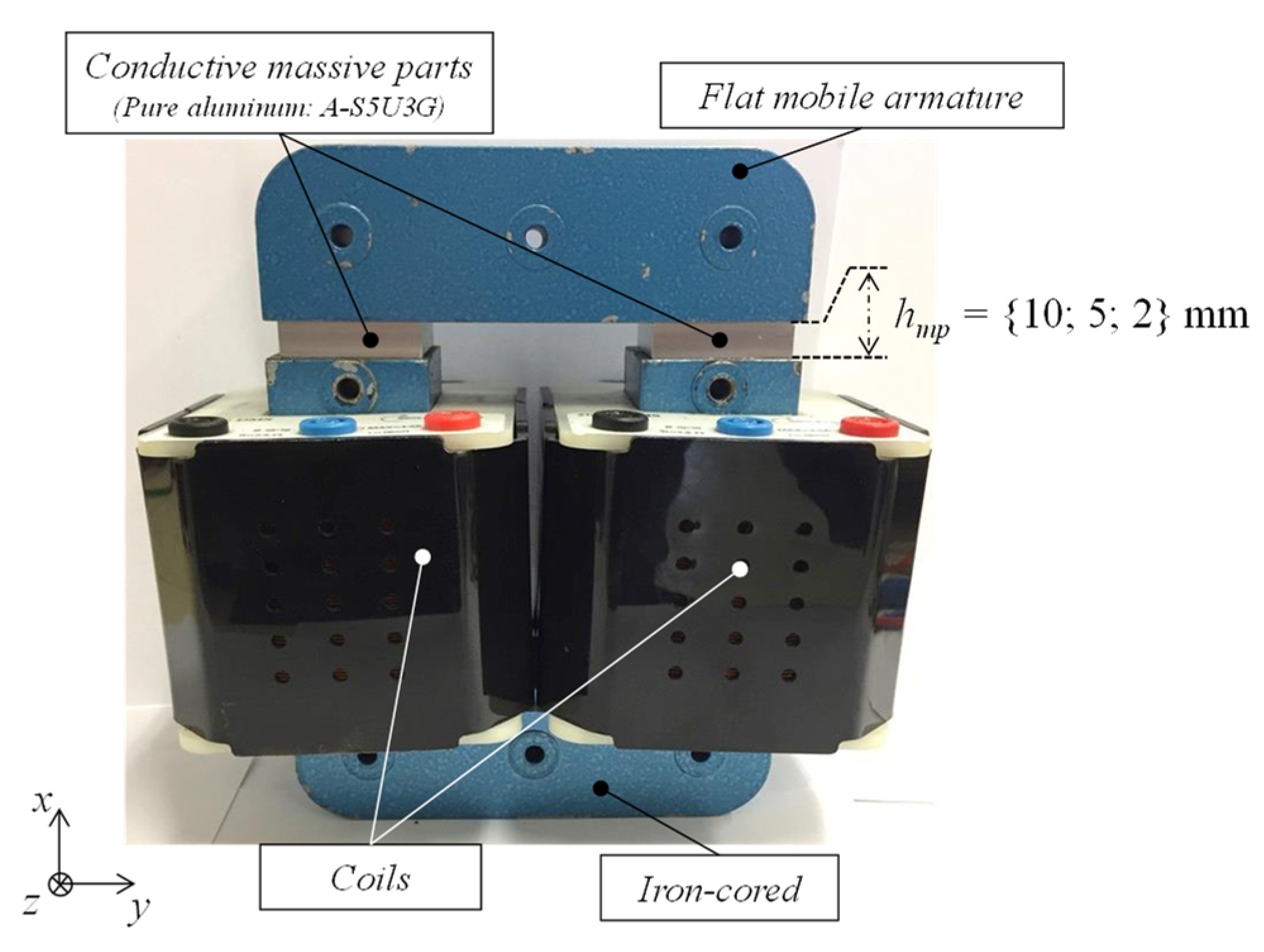
2. U-Shaped Electromagnetic Device and Conductive Massive Parts Description

2.1. Overall View

The magnetic field source is a U-shaped electromagnetic device with a flat mobile armature (or adjustable airgap), which is illustrated in Figure 1 with the rectangular-shaped aluminium conductive massive parts. The electromagnet is supplied with a sinusoidal instantaneous voltage $v$ at $f$ = 50 Hz. The ferromagnetic circuit is not saturated with the voltage levels used. Therefore, the instantaneous electrical current $i$, flowing through the coils will also be sinusoidal with a maximum amplitude of $I_{\max }$ = 4.5 A. The characteristics of the electromagnet (viz., ferromagnetic circuit and coil) are shown in Figure 2 and given in

Table 1. Parameters of the electromagnetic device.

	Symbol	Quantity	Values
Ferromagnetic circuit	$d$	Depth	46 mm
	$w$	Width	45 mm
	$h_y$	Yoke height	45 mm
	$l_y$	Yoke length	150 mm
	$h_{ot}$	Height overhang top	19 mm
	$h_{ob}$	Height overhang bot	4 mm
	${\mu }_0$	Vacuum permeability	4π10−7 H/m
	B(H)	FeSi ferromagnetic properties	Figure 3
Coils	$N_t$	Number of coils turns	500
	$I_{\max }$	Maximal current (per coil)	4.5 A
	$h_c$	Coil height	77 mm
	$w_c$	Coil width	10 mm
	$S_c=w_c\times h_c$	Conductors area	700 mm²
	$r_c$	Electrical resistance	2.8 Ω
	$L$	Inductance	18 mH

.

One of the major advantages of the flat mobile armature electromagnet compared to a Helmholtz coil is that it is possible to modify the height of the air gap $e$ in order:

• to have a more or less intense magnetic field in the air gap;
• to be able to insert conductive massive parts of various thicknesses $h_{mp}$;
• and to displace the conductive massive parts with respect to the magnetic circuit to apply a spatially non-uniform applied magnetic field to the studied materials.

The values of $e$ = $h_{mp}$ considered in this paper will be 10, 5, and 2 mm.

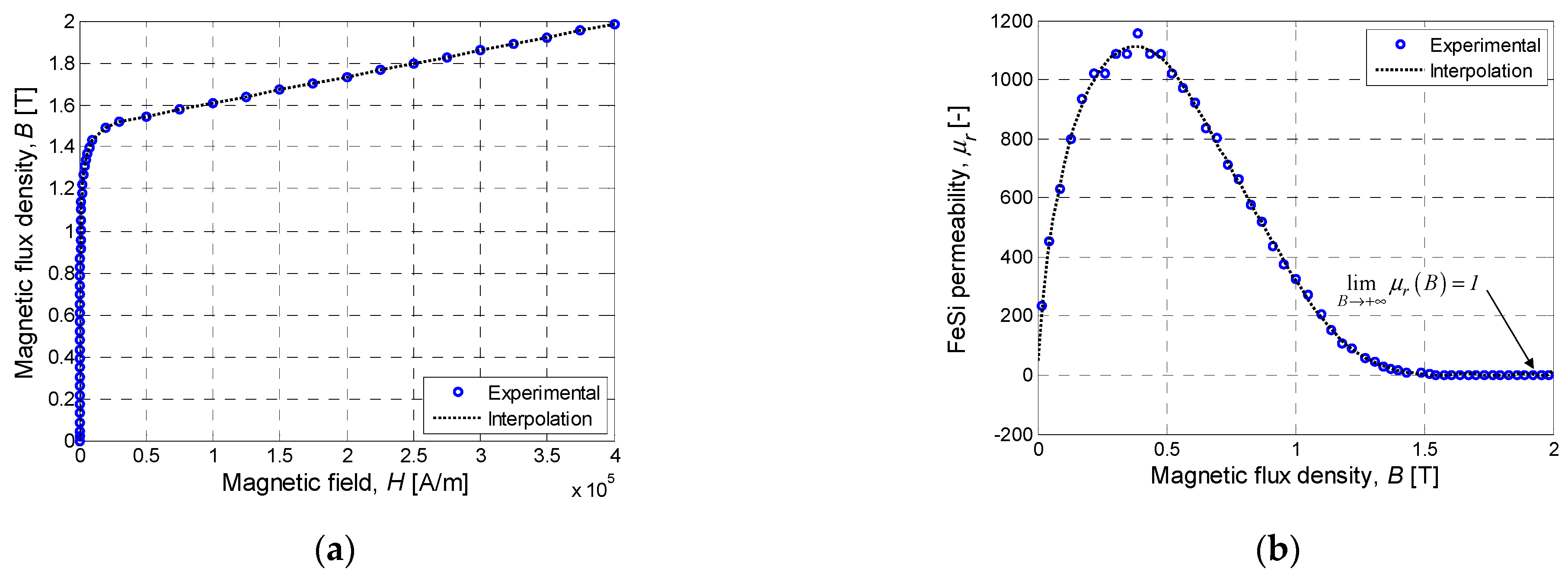
2.2. Ferromagnetic Circuit

The ferromagnetic circuit is composed of Iron Silicium (FeSi) sheets. Their magnetic properties are shown in Figure 3 (anhysteretic $B\left(H\right)$ and ${\mu }_r\left(B\right)$ curves).

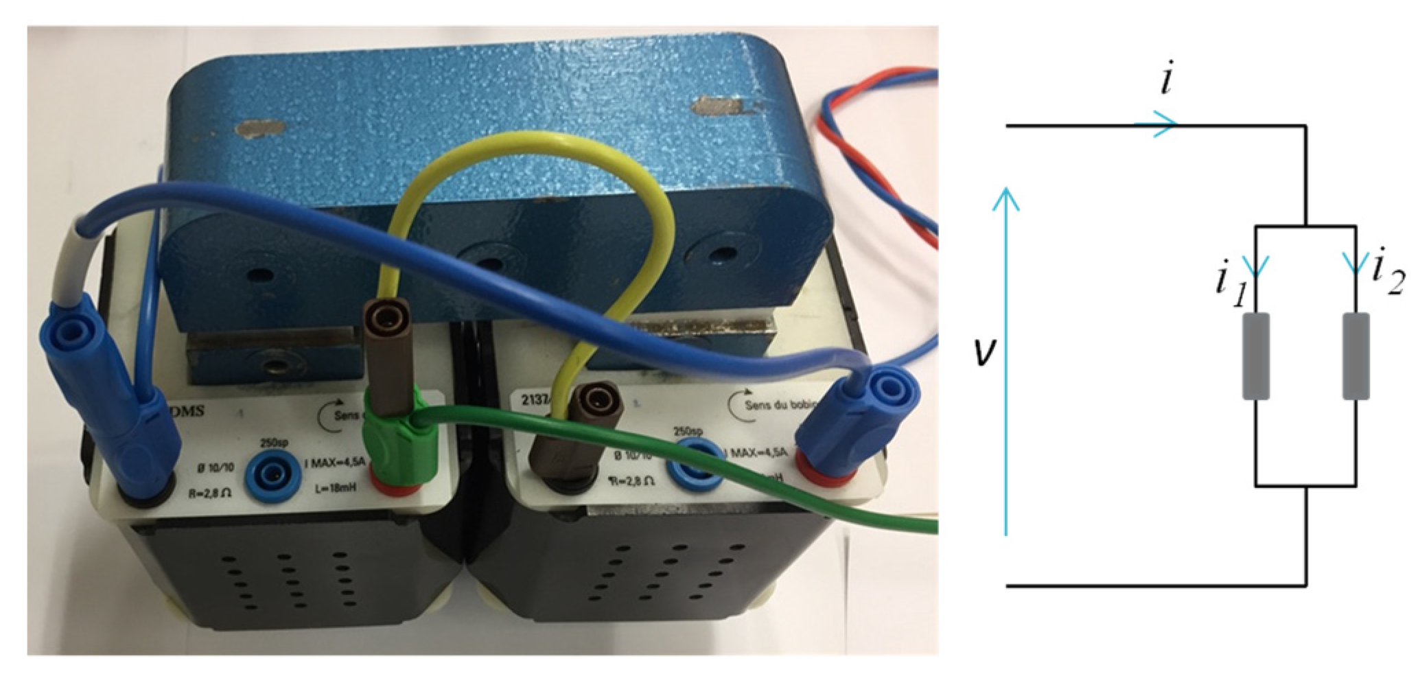
2.3. Coils and Connections

Two identical coils, having $N_t$ series of turns, are associated with the ferromagnetic circuit as shown in Figure 1. These coils create a magnetic flux linkage $\psi$ in the iron core and the conductive massive parts. The coils’ arrangement in the electromagnet allows for magnetic symmetry of fluxes (viz., principal and leakage flux). In order to obtain a maximum magnetic field in the air gap $e$ and, consequently, to measure higher eddy-current losses, the coils must be connected in parallel as shown in Figure 4.

According to Faraday–Hopkinson law, we have

$$v=R\cdot i+\omega \cdot \frac{\partial \psi }{\partial {\theta }_{rs}} \mathrm{with} {\theta }_{rs}=\omega \cdot t,$$

(4)

$$\psi =\frac{N_t{}^2}{\Re }\cdot i=L_m\cdot i,$$

(5)

where $R=r_c/2$ is the total electrical resistance for a parallel coupling with $r_c$ the electrical resistance of the coil, ${\theta }_{rs}$ is the electrical angular position, $\Re$ is the principal magnetic reluctance, and $L_m$ is the magnetizing inductance.

By assuming that the resistive part can be considered negligible compared to the inductive part, the root mean square (RMS) current $I$ and the phase shift $\phi$ (between $i$ and $v$) of $i$ are determined by

$$I\cdot e^{j\cdot \phi }\cong \frac{V}{j\cdot \omega \cdot L_m}=\frac{V}{\omega \cdot L_m}\angle -\pi /2$$

(6)

where $V$ is the RMS voltage.

It can be seen that for a given $V$, if the number of coil turns is increased, then the RMS current $I$ as well as the generated magnetic field is less important. According to (6), the phase shift $\phi$ is approximately equal to $-\pi /2$.

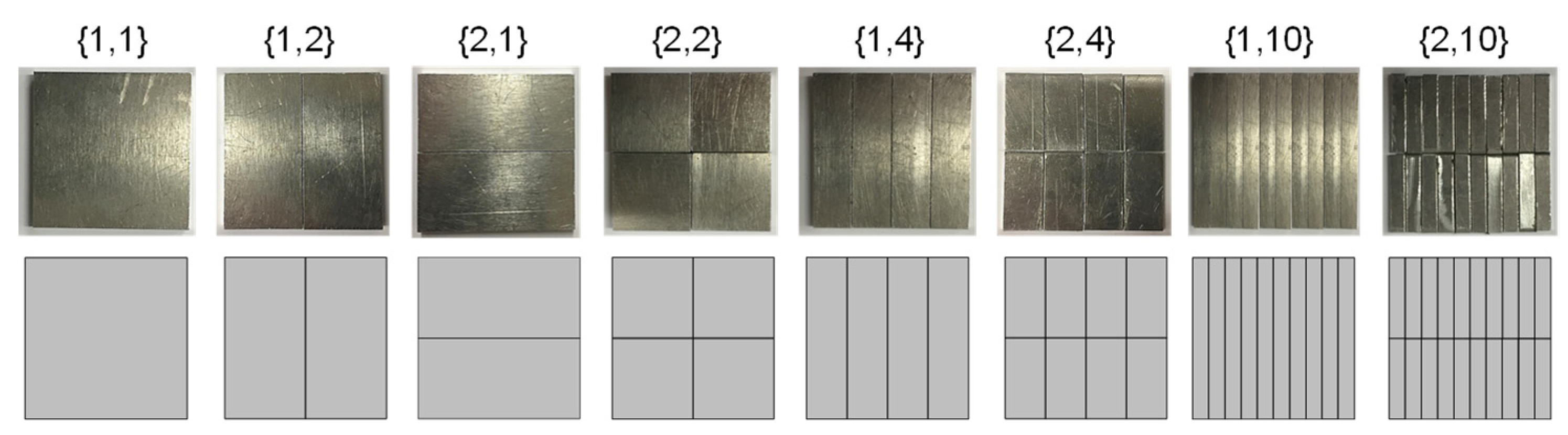
2.4. Conductive Massive Parts

This experimental device allows the characterization of $N_{mp}=2$ conductive massive parts at the same time, as illustrated in Figure 1. The flat mobile armature allows the height of the air gap $e$ to be changed and conductive massive parts to be inserted. In our study, rectangular-shaped aluminium conductive massive parts (aluminium: A-S5U3G) have been considered with ${\sigma }_{mp}={\sigma }_{Al}=20\times {10}^6$ S/m.

The segmentation effect, which is also investigated in this paper, influences the eddy currents and, therefore, the eddy-current losses. In the$yz$-plane, the conductive massive part can be decomposed into $N{s}_z\times N{s}_y$ regular conductive segments in which $N{s}_y\in {\mathbb{N}}^{\ast }$ and $N{s}_z\in {\mathbb{N}}^{\ast }$ are, respectively, the segmentation number in the $y$-axis and the $z$-axis. The various segmentations $\left\{N{s}_z,N{s}_y\right\}$ are shown in Figure 5. Furthermore, it should be noted that the various conductive segments of a conductive massive part are glued together and isolated from each other. The pitch size of the isolation is 0.06 mm (type: Ruban Kapton).

3. Applied Magnetic Field Distribution with Experimental Validations

In this section, the main objective is to precisely establish and measure the magnetic field distribution applied on the aluminium conductive massive parts generated by the electromagnet as a function of the current injected into the coils. The experimental measurements of this magnetic field will be the mean input data for the analytical model of eddy-current losses.

3.1. Instrumentation

3.1.1. Hall Effect Sensor

The value of the magnetic field in the air gap is obtained by using a Hall effect sensor HE144T (Asensor Technology AB^® [35]). This sensor, with an estimated uncertainty of 1%, is shown in Figure 6a. One of the advantages of this sensor is its thickness, which is only 0.5 mm. This Hall effect sensor has four pins, two to supply the probe with a direct current of 1 mA, and two to measure the Hall voltage and recover the value of the measured magnetic field.

In order to power a 1 mA probe, an electrical circuit diagram (supplied with −15 V/0 V/15 V) was created and developed with the Proteus Isis software (Version 8.2, Société Labcenter Electronics, France). Subsequently, EuroCircuits^® was used to fabricate printed circuits (single track cards) onto which various components were soldered to obtain the final version presented in Figure 6b. In order to measure the magnetic field on a given path quickly and precisely, a total of 12 Hall effect sensors was determined to be the optimal and cost-effective choice. Figure 6b presents the created power/acquisition box, which can contain 12 printed circuits. In order to observe the magnetic field signals, the sensors’ outputs are connected to the BNC cables, which can be directly connected to an oscilloscope.

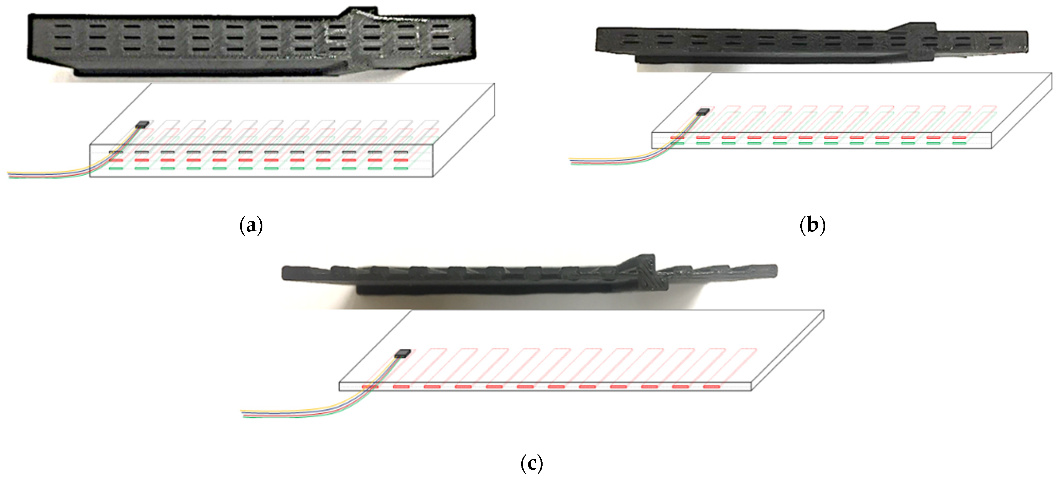
3.1.2. Sensor Supports

Various supports have been realized to make it possible to measure the magnetic field very precisely at regular intervals, as shown in Figure 7. These supports (non-magnetic and non-conductive) are produced by 3D printing in PolyLactic Acid (PLA). The thickness of the measuring supports must be the same as the thickness of the conductive massive parts (viz., $e=h_{mp}$) so that the magnetic field in the air gap can be measured correctly for the eddy-current loss calculation.

Figure 8 presents the various supports and their arrangements according to the desired air-gap thickness. For $e=10$ mm (Figure 8a), it was possible to make three layers of 12 slots (i.e., 36 measurement locations). When $e=5$ mm (Figure 8b), the support is composed of two layers of 12 slots (i.e., 24 measurement locations). For the final support of $e=2$ (Figure 8c), the printing method was modified to solve the problem related to the thinness of the geometry, and only 12 measurements were possible.

3.2. Experimental Measurements

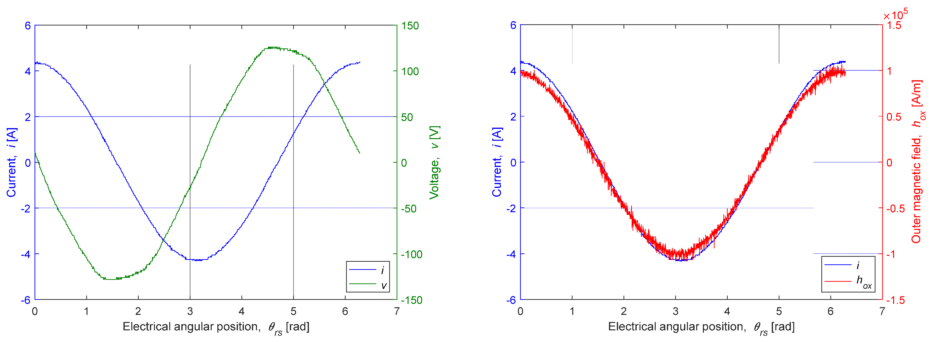
3.2.1. Temporal Evolutions of $i$, $v$, and $h_{ox}$

It is possible to visualize the temporal evolutions over an electrical period of the different quantities such as the current $i$, the voltage $v$, and the normal magnetic field at the sensor support $h_{ox}$. The measurements are realized for $I$ = 3 A (viz., $V$ = 90 V). The various temporal evolutions for a 10 mm air gap are shown in Figure 9.

By comparing the various curves, some generalities could be made:

• $i$ and $v$ (only the fundamental components) have a phase shift $\phi$ of $\approx -\pi /2$ as demonstrated by (6);
• $i$ and $h_{ox}$ are still in phase.

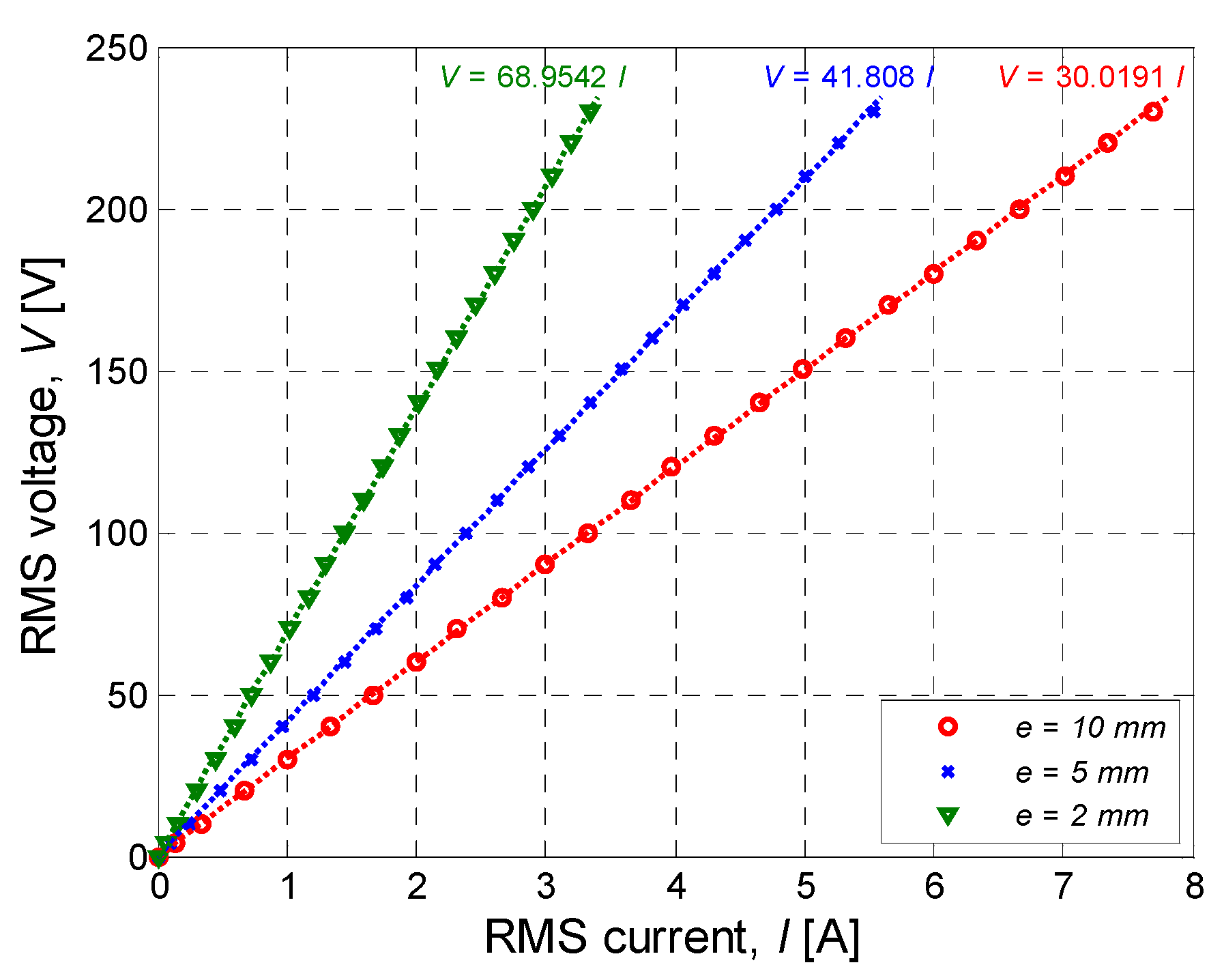
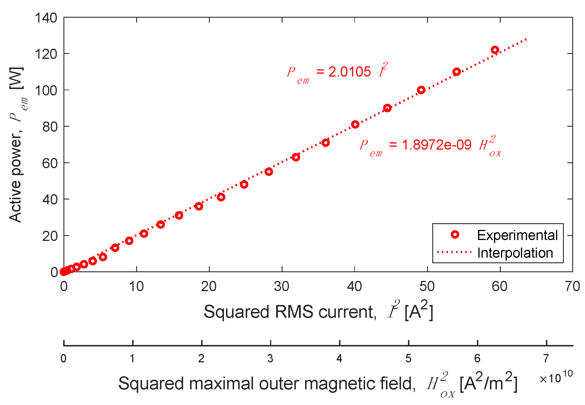
3.2.2. Linear Dependency of $V\left(I\right)$ and $H_{ox}\left(I\right)$

The electromagnet is voltage-controlled, for an RMS voltage $V$ varying from 0 to 230 V in 10 V steps, the RMS current $I$ flowing in the coils is measured.

Figure 10 shows the dependence between $V$ and $I$ for the three air-gap thicknesses detailed previously. It can be seen that, for a given $V$, when $e$ increases (equivalent to a decrease in the magnetizing inductance $L_m$), $I$ also increases. Moreover, $V$ is proportional to $I$ for the various thicknesses, and it could be deduced that the device does not saturate.

Concerning the measured maximum magnetic field, $H_{ox}$, the measurements are performed in the middle of the air gap for the three air-gap thicknesses. Figure 11 shows the dependence between $H_{ox}$ and $I$. It can be seen that, for a given $I$, when $e$ increases, $H_{ox}$ decreases. The generated maximum magnetic field $H_{ox}$ is therefore the image of $I$. These conclusions are confirmed by (assuming that ${\mu }_r\to +\infty$)

$$H_{ox}\cong \frac{N_t\sqrt{2}}{2\cdot e}\cdot I \left(\mathit{resulting\; from\; Hopkinson’s\; law}\right).$$

(7)

It is interesting to note that the slopes, as well as the ratios between the various curves in Figure 11, can be validated by (7).

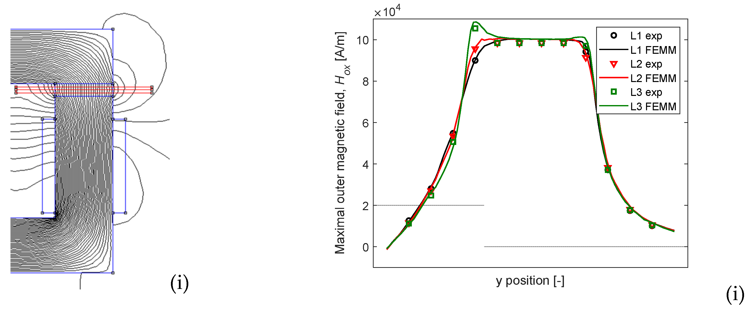
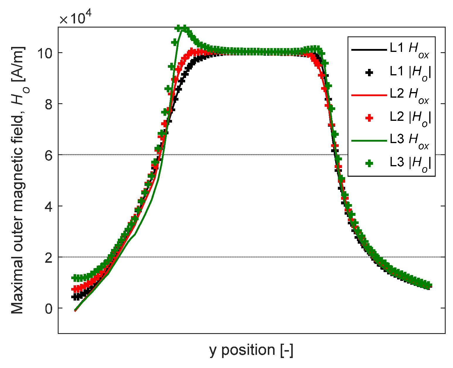
3.2.3. Spatial Evolution of $H_{ox}$

The study aims to determine the spatial distribution of the magnetic field generated in the air gap along the flux paths (or sensor support layers) (see Figure 8). Figure 12 presents the spatial distribution of the measured maximum magnetic field $H_{ox}$ for a 10 mm air gap at the various layers (that is 36 measurement locations). The measurements are realized for $I$ = 3 A (viz., $V$ = 90 V). It can be observed that $H_{ox}$ is homogeneous (or spatially uniform) throughout the air gap with a value close to 100 kA/m. Moreover, due to leakage fluxes, the levels of $H_{ox}$ are different at the edges (the right and the left sides of the air gap) and in the middle of the air gap. The magnetic leakages are more important inside the electromagnet than outside at the air gap and can be assumed to be negligible.

3.3. Comparison between Measurements and Numerical Results

The objective here is to perform a comparative analysis of the magnetic generated in the air gap (without the conductive massive parts) between the experimental measurements and the numerical results, in order to evaluate the effectiveness of the mean input data for the eddy-current loss model.

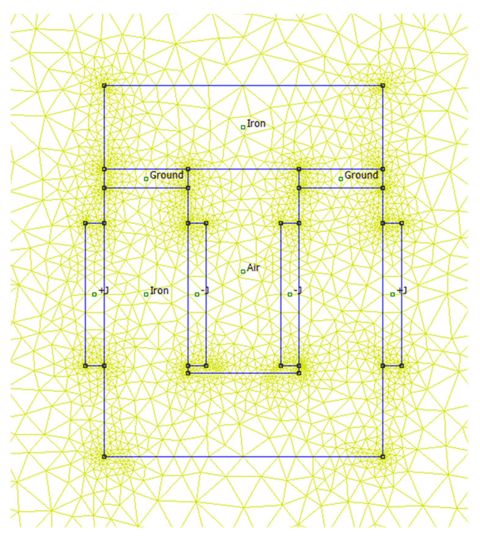
3.3.1. Numerical Modeling

The numerical model, under the FEMM software [34], considers the electromagnet without the conductive massive parts introduced previously (see Figure 2 and Figure 7). A calculation code developed using the Matlab^® environment allows us to execute commands in the FEMM software, as illustrated in Figure 13.

The assumptions used in the static numerical model are:

• the model is supposed to be in 2D (i.e., the end effects are neglected);
• the magnetic materials are considered to be isotropic;
• the hysteresis effect is ignored;
• and the skin effect in all materials (e.g., copper and iron) is neglected.

The 2D numerical mesh (with 7463 nodes) of the electromagnet is illustrated in Figure 14. The numerical simulations are performed for the three air-gap thicknesses with $I$ = 3 A (viz., $V$ = 90 V) and by using the FeSi ferromagnetic properties (see Figure 3).

3.3.2. Results Discussion

Figure 15a presents the equipotential lines ($\approx$90 lines) of the magnetic vector potential in the electromagnet with the 2D numerical modeling. The validation paths of the maximum magnetic field $H_{ox}$ for the comparison are given in Figure 15a (equivalent to various layers in Figure 8). The spatial evolution of $H_{ox}$ are represented on the various paths in Figure 15b. The solid lines represent $H_{ox}$ computed by the 2D numerical modeling and the symbols correspond to experimental measurements. It can be seen that a very good agreement between the experimental measurements and the numerical results is obtained whatever the validation paths and the air-gap thickness. By observing the equipotential lines, it could be concluded that a decrease in the air-gap thickness reduces the leakage fluxes, and thus, a more uniform magnetic field is observable in the active part of the electromagnetic (such as the transition of Figure 15a(i) to Figure 15b(iii). At the extremities, the magnetic field decreases faster.

The normal component $H_{ox}$ and the module $\left|H_o\right|$ of the magnetic field in the air gap are plotted in Figure 16. The studied case is the following: a 10 mm air gap (maximum leakage), and an RMS current $I$ = 3 A (viz., $V$ = 90 V). By comparing the magnetic field values obtained from the numerical modeling, the similar evolutions of $H_{ox}$ and $\left|H_o\right|$ could be observed for all the studied paths. This confirms that the normal component $H_{ox}$ of the magnetic field is predominant. Eddy currents are induced only by the normal component $H_{ox}$ and the effects of the tangential component $H_{oy}$ on the eddy-current loss calculation can be neglected.

4. Eddy-Current Loss Calculation with Experimental Validations

In this section, the main objective is to estimate analytically and experimentally the volumic eddy-current losses in rectangular-shaped aluminium conductive massive parts generated by a varying applied magnetic field (see Section 3).

4.1. Analytical Model

4.1.1. Introduction

The analytical model is based on the formal resolution of the magnetodynamic Maxwell’s equations in Cartesian coordinates $\left(x,y,z\right)$ by using the separation of variables method and the Fourier series. By applying boundary conditions (BCs) to the edges of the conductive massive part, the inner (or resulting) magnetic field in the conductive massive parts considering the skin effect can be obtained analytically. From this quantity, the resultant eddy-current density distribution as well as the eddy-current losses can be determined analytically. These losses have been established from Poynting’s theorem. The segmentation effect in both directions (i.e., $y$-axis and $z$-axis) is also considered in the mathematical development of the analytical model.

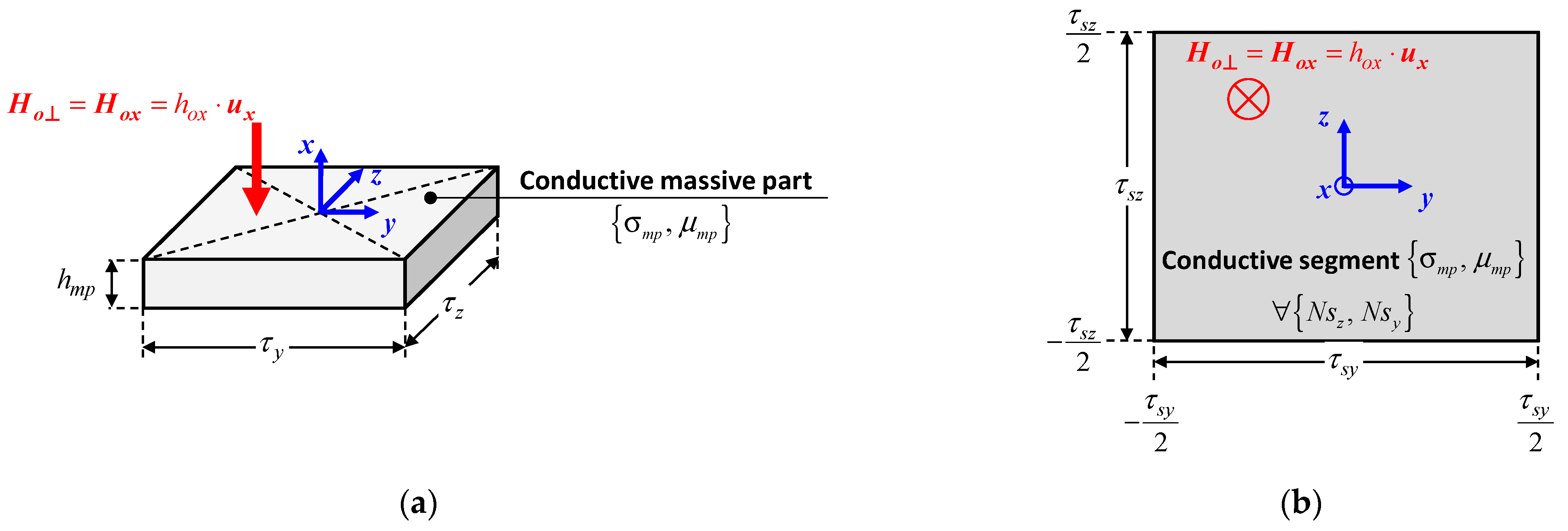
4.1.2. Assumptions and Segmentation

Figure 17a represents the geometrical/physical parameters of the conductive massive part and the coordinate system used. The simplifying assumptions are:

• the studied materials are excited by a spatially uniform outer magnetic field supposed normal to the $yz$-plane, as shown in Figure 17a; i.e., ${\mathit{H}}_{\mathit{o}}=\left\{{\mathit{H}}_{\mathit{o}\perp }\hspace{0.33em};0\hspace{0.33em};\hspace{0.33em}0\right\}$ with ${\mathit{H}}_{\mathit{o}\perp }={\mathit{H}}_{\mathit{o}\mathit{x}}=h_{ox}\cdot {\mathit{u}}_{\mathit{x}}$ where $\mathit{u}$ is the unity vector of the three components;
• the eddy currents are induced only by $h_{ox}$ and the effects of other magnetic field components on the eddy-current loss calculation can be neglected;
• the studied materials are rectangular-shaped only and considered to be isotropic (i.e., the magnetic permeability ${\mu }_{mp}$ and the electrical conductivity ${\sigma }_{mp}$ of the conductive massive part are constant);
• and ${\sigma }_{mp}$ is assumed to be invariant to the operating temperature.

Regarding the last assumption, even if the temperature of the conductive massive part varies, the maximum increase (<4%) of ${\sigma }_{mp}$ (viz., $20\times {10}^6<{\sigma }_{mp}<20.8\times {10}^6$ S/m) will not have a significant influence on the eddy-current losses.

In Section 3, it was demonstrated that:

• the leakage fluxes at the edges of the conductive massive parts could be neglected (such as $h_{ox}$ is independent of x, $\forall h_{mp}$);
• and the electromagnet supplied with a sinusoidal voltage was not saturated.
• Therefore, the analytical model can be developed in 2D and the $yz$-plane. Hence,
• the resultant eddy-current density has two components, i.e., ${\mathit{J}}_{\mathit{\sigma }}=\left\{0;{\mathit{J}}_{\mathit{\sigma }\mathit{y}};{\mathit{J}}_{\mathit{\sigma }\mathit{z}}\right\}$ with ${\mathit{J}}_{\mathit{\sigma }\mathit{y}}=j_{\sigma y}\cdot {\mathit{u}}_{\mathit{y}}$ and ${\mathit{J}}_{\mathit{\sigma }\mathit{z}}=j_{\sigma z}\cdot {\mathit{u}}_{\mathit{z}}$;
• and the inner (or resulting) magnetic field in the conductive massive parts considering the skin effect ${\mathit{H}}_{\mathit{i}}=\left\{{\mathit{H}}_{\mathit{i}\mathit{x}}\hspace{0.33em};0\hspace{0.33em};\hspace{0.33em}0\right\}$ with ${\mathit{H}}_{\mathit{i}\mathit{x}}=h_{ix}\cdot {\mathit{u}}_{\mathit{x}}$.

In the unsaturated state, all electromagnetic quantities can be considered to be sinusoidal, i.e.,

$$q=\mathrm{Re}\left\{Q\cdot e^{j\cdot {\theta }_{rs}}\right\} \mathrm{with} j=\sqrt{-1}$$

(8)

where $Q$ is the maximum complex amplitude of $q$.

The segmentation effect influences the eddy currents, and therefore, the eddy-current losses. Figure 17b shows a conductive segment whose geometrical parameters are defined by

$${\tau }_{sy}=\frac{{\tau }_y}{N{s}_y} \mathrm{and} {\tau }_{sz}=\frac{{\tau }_z}{N{s}_z}.$$

(9)

For $N{s}_z\times N{s}_y=1\times 1$, the conductive massive part is not segmented. In Section 3, it was observed that $h_{ox}$ applied to the studied materials was homogeneous (or spatially uniform) over the whole piece. Therefore, the inner (or resulting) magnetic field $h_{ix}$, the distribution of ${\mathit{J}}_{\mathit{\sigma }}$, as well as the eddy-current losses, can be considered identical in each conductive segment, $\forall \left\{N{s}_z,N{s}_y\right\}$. It is interesting to note that this remark is no longer valid when $h_{ox}$ is spatially non-uniform because the eddy-current losses would be more or less different in each conductive segment.

4.1.3. Resulting Magnetic Field

➢

Governing Partial Differential Equation (PDE) in Cartesian Coordinate$\left(\mathit{y},\mathit{z}\right)$: In the quasi-stationary approximation, inside a linear (non)magnetic material without electromagnetic sources, the magnetodynamic PDE in terms of $h_{ix}$, resulting from Maxwell’s equations, is defined by

$${\nabla }^2{h}_{ix}-{\mu }_{mp}\cdot {\sigma }_{mp}\cdot \omega \cdot \frac{\partial h_{ix}}{\partial {\theta }_{rs}}=0 \left(\mathit{Diffusion\; equation}\right).$$

(10)

Using (7), (9) becomes, in complex notation

$${\nabla }^2{H}_{ix}-{\alpha }_{mp}{}^2\cdot H_{ix}=0 \left(\mathit{Helmholtz’s\; equation}\right)$$

(11)

$${\alpha }_{mp}=\sqrt{j\cdot {\mu }_{mp}\cdot {\sigma }_{mp}\cdot \omega }=\frac{1+j}{{\delta }_{mp}}$$

(12)

where ${\delta }_{mp}$ is the skin depth of the conductive massive part defined by (1), and ${\nabla }^2{H}_{ix}$ is the complex Laplacian of $h_{ix}$ in the $yz$-plane

$${\nabla }^2{H}_{ix}=\frac{{\partial }^2{H}_{ix}}{\partial y^2}+\frac{{\partial }^2{H}_{ix}}{\partial z^2}.$$

(13)

By using the separation of variables method, the 2D general solution of $H_{ix}$ in both directions (i.e., $y$-axis and $z$-axis) can be defined by a complex Fourier series [1]. The unknown coefficients are determined analytically from the BCs at the edges of each conductive segment.

➢

Definition of BCs: Since the conductive massive parts are excited by an outer sinusoidal spatially uniform magnetic field, the BCs can be considered homogeneous [see Section 3] and equal to $-H_{ox}$ (according to the Cartesian coordinates of Figure 17) on the edges, $\forall \left\{N{s}_z,N{s}_y\right\}$:

-

in the $y$-axis:

$$h_{ix}\left(y,\pm \frac{{\tau }_{sz}}{2},{\theta }_{rs}\right)=h_{ox}\Rightarrow H_{ix}\left(y,\pm \frac{{\tau }_{sz}}{2}\right)=-H_{ox},$$

(14)

-

in the $z$-axis:

$$h_{ix}\left(\pm \frac{{\tau }_{sy}}{2},z,{\theta }_{rs}\right)=h_{ox}\Rightarrow H_{ix}\left(\pm \frac{{\tau }_{sy}}{2},z\right)=-H_{ox}.$$

(15)

Nevertheless, it is interesting to note that imposing $-H_{ox}$ as a BC on the edges remains a more or less rigorous approximation (e.g., the negligible magnetic leakages, etc.).

➢

Magnetic Field Solution: By satisfying (14) and (15), the 2D final solution of $H_{ix}$ (viz., the complex amplitude of $h_{ix}$) in each conductive segment can be written as a Fourier series

$$H_{ix}=-H_{ox}\cdot \left[\frac{\mathrm{c}\mathrm{o}\mathrm{s}\mathrm{h}\left({\alpha }_{mp}\cdot z\right)}{\mathrm{c}\mathrm{o}\mathrm{s}\mathrm{h}\left({\alpha }_{mp}\cdot \frac{{\tau }_{sz}}{2}\right)}+{\displaystyle \sum _n{e}_n\cdot \mathrm{c}\mathrm{o}\mathrm{s}\mathrm{h}\left({\lambda }_n{}^{\prime }\cdot y\right)\cdot \mathrm{c}\mathrm{o}\mathrm{s}\mathrm{h}\left({\lambda }_n\cdot z\right)}\right],$$

(16)

$$e_n=2\cdot {\left(\frac{{\alpha }_{mp}}{{\lambda }_n{}^{\prime }}\right)}^2\cdot \frac{\mathrm{s}\mathrm{i}\mathrm{n}\mathrm{c}\left({\lambda }_n\cdot \frac{{\tau }_{sz}}{2}\right)}{\mathrm{c}\mathrm{o}\mathrm{s}\mathrm{h}\left({\lambda }_n{}^{\prime }\cdot \frac{{\tau }_{sy}}{2}\right)} \mathrm{with} {\lambda }_n{}^{\prime }=\sqrt{{\alpha }_{mp}{}^2+{\lambda }_n{}^2},$$

(17)

where ${\lambda }_n=n\cdot \pi /{\tau }_{sz}$ is the spatial frequency (or periodicity) of $H_{ix}$ with $n\in \left\{{\mathbb{N}}^{*},N_{\max }|odd\right\}$ the spatial harmonic orders in which $N_{\max }$ is the finite number of spatial harmonics terms.

4.1.4. Resultant Eddy-Current Density Distribution

According to the superposition principle, the magnetic field due to eddy currents $H_{\sigma }=\left\{H_{\sigma x}\hspace{0.33em};0\hspace{0.33em};\hspace{0.33em}0\right\}$ with $H_{\sigma x}=h_{\sigma x}\cdot u_x$ is defined by

$$h_{\sigma x}=h_{ix}-h_{ox}\Rightarrow H_{\sigma x}=H_{ix}-H_{ox}.$$

(18)

From the Maxwell–Ampère law (i.e., $J_{\sigma }=\nabla \times H_{\sigma }$), the complex amplitudes of $j_{\sigma y}$ and $j_{\sigma z}$ in each conductive segment are respectively given by

$$J_{\sigma y}=H_{ox}\cdot \left[{\alpha }_{mp}\cdot \frac{\mathrm{s}\mathrm{i}\mathrm{n}\mathrm{h}\left({\alpha }_{mp}\cdot z\right)}{\mathrm{c}\mathrm{o}\mathrm{s}\mathrm{h}\left({\alpha }_{mp}\cdot \frac{{\tau }_{sz}}{2}\right)}-{\displaystyle \sum _n{e}_n\cdot {\lambda }_n\cdot \mathrm{c}\mathrm{o}\mathrm{s}\mathrm{h}\left({\lambda }_n{}^{\prime }\cdot y\right)\cdot \mathrm{s}\mathrm{i}\mathrm{n}\left({\lambda }_n\cdot z\right)}\right],$$

(19)

$$J_{\sigma z}=H_{ox}\cdot {\displaystyle \sum _n{e}_n\cdot {\lambda }_n{}^{\prime }\cdot \mathrm{s}\mathrm{i}\mathrm{n}\mathrm{h}\left({\lambda }_n{}^{\prime }\cdot y\right)\cdot \mathrm{c}\mathrm{o}\mathrm{s}\left({\lambda }_n\cdot z\right)}.$$

(20)

4.1.5. Volumic Eddy-Current Losses

The complex time-averaged Poynting vector over time in each conductive segment is defined by

$$〈{\Pi }_{cs}〉=\frac{1}{2\cdot {\sigma }_{mp}}\cdot \left(J_{\sigma }\times \overline{H_i}\right)=\frac{1}{2\cdot {\sigma }_{mp}}\cdot \left(\begin{array}{c}0\\ J_{\sigma z}\cdot \overline{H_{ix}}\\ -J_{\sigma y}\cdot \overline{H_{ix}}\end{array}\right).$$

(21)

According to Poynting’s theorem, $〈{\Pi }_{cs}〉$ across a closed surface $S$ is given by the complex Poynting vector flux through this surface. From (14), (15) and (21), we obtain

$$〈{\Pi }_{cs}〉={\displaystyle {∯}_S〈{\Pi }_{cs}〉\cdot }dS=\frac{h_{mp}}{{\sigma }_{mp}}\cdot \left[{\displaystyle \underset{-\frac{{\tau }_{sz}}{2}}{\overset{\frac{{\tau }_{sz}}{2}}{\int }}{\left(J_{\sigma z}\cdot \overline{H_{ix}}\right)}_{y=-\frac{{\tau }_{sy}}{2}}\cdot dz}-{\displaystyle \underset{-\frac{{\tau }_{sy}}{2}}{\overset{\frac{{\tau }_{sy}}{2}}{\int }}{\left(J_{\sigma y}\cdot \overline{H_{ix}}\right)}_{z=\frac{{\tau }_{sz}}{2}}\cdot dy}\right].$$

(22)

After the development, by substituting (16), (17), (19) and (20) into (22), the time-averaged apparent power in each conductive segment is then given by, $\forall \left\{N{s}_z,N{s}_y\right\}$,

$$〈{\Pi }_{cs}〉=P_{cs}+j\cdot Q_{cs}=2\cdot \frac{h_{mp}\cdot {\left|H_{ox}\right|}^2}{{\sigma }_{mp}}\cdot \left(g_0+{\displaystyle \sum _n{g}_n}\right),$$

(23)

$$g_0={\alpha }_{mp}\cdot \frac{{\tau }_{sy}}{2}\cdot \frac{\mathrm{s}\mathrm{i}\mathrm{n}\mathrm{h}\left({\alpha }_{mp}\cdot \frac{{\tau }_{sz}}{2}\right)}{\mathrm{c}\mathrm{o}\mathrm{s}\mathrm{h}\left({\alpha }_{mp}\cdot \frac{{\tau }_{sz}}{2}\right)},$$

(24)

$$g_n=\frac{2}{\frac{{\tau }_{sz}}{2}}\cdot \frac{{\lambda }_n{}^{\prime }}{{\lambda }_n{}^2}\cdot {\left(\frac{{\alpha }_{mp}}{{\lambda }_n{}^{\prime }}\right)}^4\cdot \frac{\mathrm{s}\mathrm{i}\mathrm{n}\mathrm{h}\left({\lambda }_n{}^{\prime }\cdot \frac{{\tau }_{sy}}{2}\right)}{\mathrm{c}\mathrm{o}\mathrm{s}\mathrm{h}\left({\lambda }_n{}^{\prime }\cdot \frac{{\tau }_{sy}}{2}\right)},$$

(25)

where $P_{cs}=\mathrm{Re}\left\{〈{\Pi }_{cs}〉\right\}$ and $Q_{cs}=\mathrm{Im}\left\{〈{\Pi }_{cs}〉\right\}$ are the active and reactive power for each conductive segment, respectively.

It is interesting to note that the time-averaged apparent power in the rectangular-shaped conductive massive parts is calculated by

$$〈{\Pi }_{mp}〉=N_{mp}\cdot N{s}_z\cdot N{s}_y\cdot 〈{\Pi }_{cs}〉=P_{mp}+j\cdot Q_{mp}.$$

(26)

where $N_{mp}$ is the number of studied materials within the electromagnet.

4.2. Experimental Validations

4.2.1. Power Conservation Method

The process used to experimentally determine the eddy-current losses is the power conservation method. Firstly, the experimental measures must allow the characterization of the electromagnet in terms of power consumption. The various types of power measured are:

• $P_{em}$: the power consumed only by the electromagnet (i.e., without the studied materials);
• and, $P_{tot}$: the total power consumed by the electromagnet associated with the conductive massive parts.

In order to carry out compliant measurements of the power, it is necessary to respect

$${\displaystyle {\oint }_{C}H\cdot dl}={\displaystyle \sum N_t\cdot i} \left(\mathit{Ampère’s\; theorem}\right)$$

(27)

to keep the circulation length of the main magnetic flux with and without the conductive massive parts (see Figure 18). The studied materials are replaced by PLA. These supports (non-magnetic and non-conductive) are produced by 3D printing (see Section 3). According to (27), the PLA thickness should be equal to the height of conductive massive parts, as shown in Figure 18.

Finally, from these data, the volumic eddy-current losses in the conductive massive parts can be deduced from

$$P_{mp}=P_{tot}-P_{em} \left(\mathit{Boucherot’s\; theorem}\right).$$

(28)

It is interesting to note that the electromagnet is voltage-controlled, for an RMS voltage $V$ varying from 0 to 230 V with 10 V steps, the RMS current $I$ flowing in the coils is measured. Therefore, $P_{em}$ and $P_{tot}$ were measured for the same values of $I$ and for the three air-gap thicknesses. The measurements are realized with a MetraHit 29S wattmeter.

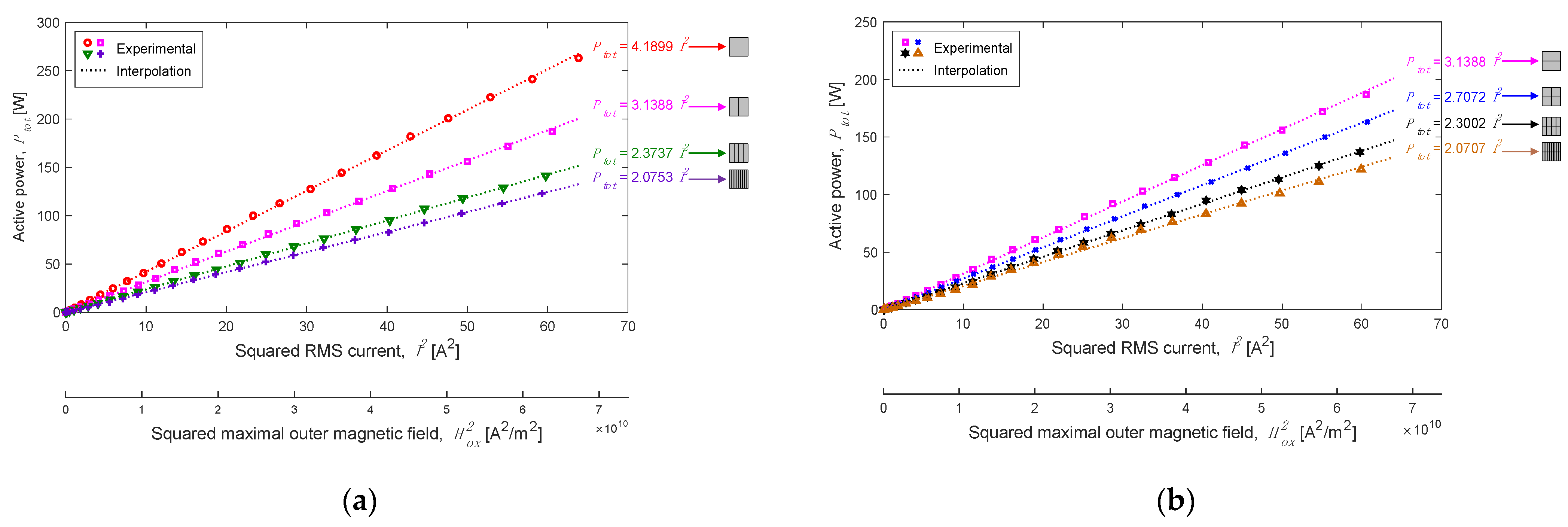
4.2.2. Power Experimental Measurements

➢

Electromagnet Power Consumption: First, the electromagnetic device alone is characterized (see Figure 18a). The active power $P_{em}$ (without the conductive massive parts replaced by PLA) is then measured.

In Section 3 (see Figure 11), it was demonstrated that $H_{ox}$ in the conductive massive parts was the image of $I$. Hence, as an example, Figure 19 permits the visualization of $P_{em}$ according to the squared RMS current $I^2$ and also the squared maximal outer magnetic field $H_{ox}{}^2$ for a 10 mm air gap. It can be observed that $P_{em}$ is proportional to $I^2$ and $H_{ox}{}^2$, $\forall e$. Moreover, from (7), for a given $I^2$, $P_{em}$ increases when $e$ decreases. A power limitation due to the power supply can also be observed.

➢

Total Power: Secondly, the conductive massive parts with(out) segmentation are introduced into the adjustable air gap. The total active power $P_{tot}$ consumed by the electromagnet associated with the conductive massive parts (see Figure 18b) is then measured.

As an example, Figure 20 shows $P_{tot}$ according to $I^2$ and $H_{ox}{}^2$ for conductive massive parts of 10 mm thickness and the various segmentations $\left\{N{s}_z,N{s}_y\right\}$ (Figure 5). It can be observed that $P_{tot}$ is also proportional to $I^2$ and $H_{ox}{}^2$, $\forall h_{mp}$. For a given $I^2$, $P_{tot}$ is less important for high thickness, $\forall \left\{N{s}_z,N{s}_y\right\}$. It is interesting to note that $P_{tot}$ decreases with the increase in the number of conductive segments in conductive massive parts, $\forall h_{mp}$.

4.2.3. Analytical and Experimental Comparison of Volumic Eddy-Current Losses

➢

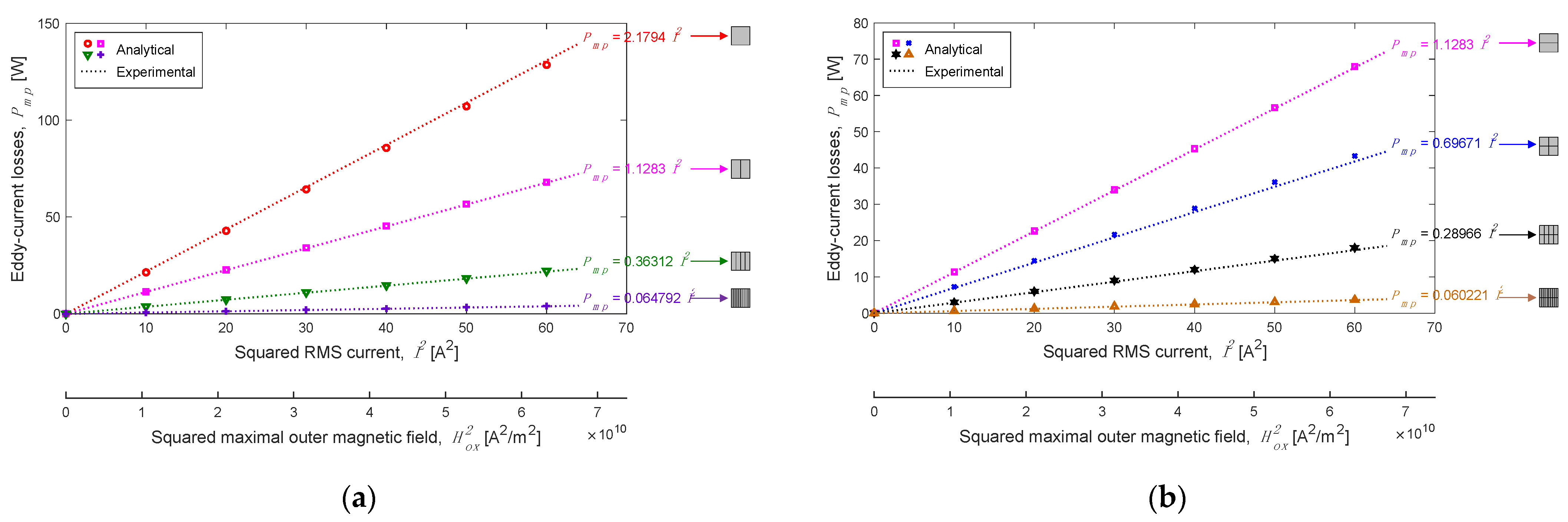
Linear Dependency: Knowing $P_{em}$ and $P_{tot}$, the volumic eddy-current losses in conductive massive parts $P_{mp}$ are determined from (26).

As an example, Figure 21 shows $P_{mp}$ according to $I^2$ and $H_{ox}{}^2$ for conductive massive parts of 10 mm thickness and for the various segmentations $\left\{N{s}_z,N{s}_y\right\}$ (see Figure 5). The analytical results are in good agreement with the experimental measurements with a maximum error of less than 5%. The difference between the analytical and experimental results can be linked to $\forall h_{mp}$:

-

the experimental method;

-

and the variation of ${\sigma }_{mp}$ due to the heating of the conductive massive parts (which is assumed to be invariant to the operating temperature in the analytical model).

It can be observed that $P_{mp}$ are proportional to $I^2$ and $H_{ox}{}^2$, $\forall h_{mp}$. This can be explained by (23), (24) and (25). Under the applied conditions, for a sinusoidal spatially uniform applied magnetic field with $f$ = 50 Hz, when the conductive massive parts are segmented, $P_{mp}$ decrease, $\forall h_{mp}$. By inserting (7) into (23), (24) and (25), it is interesting to note that $P_{mp}$ is inversely proportional to $h_{mp}$, $\forall \left\{N{s}_z,N{s}_y\right\}$.

➢

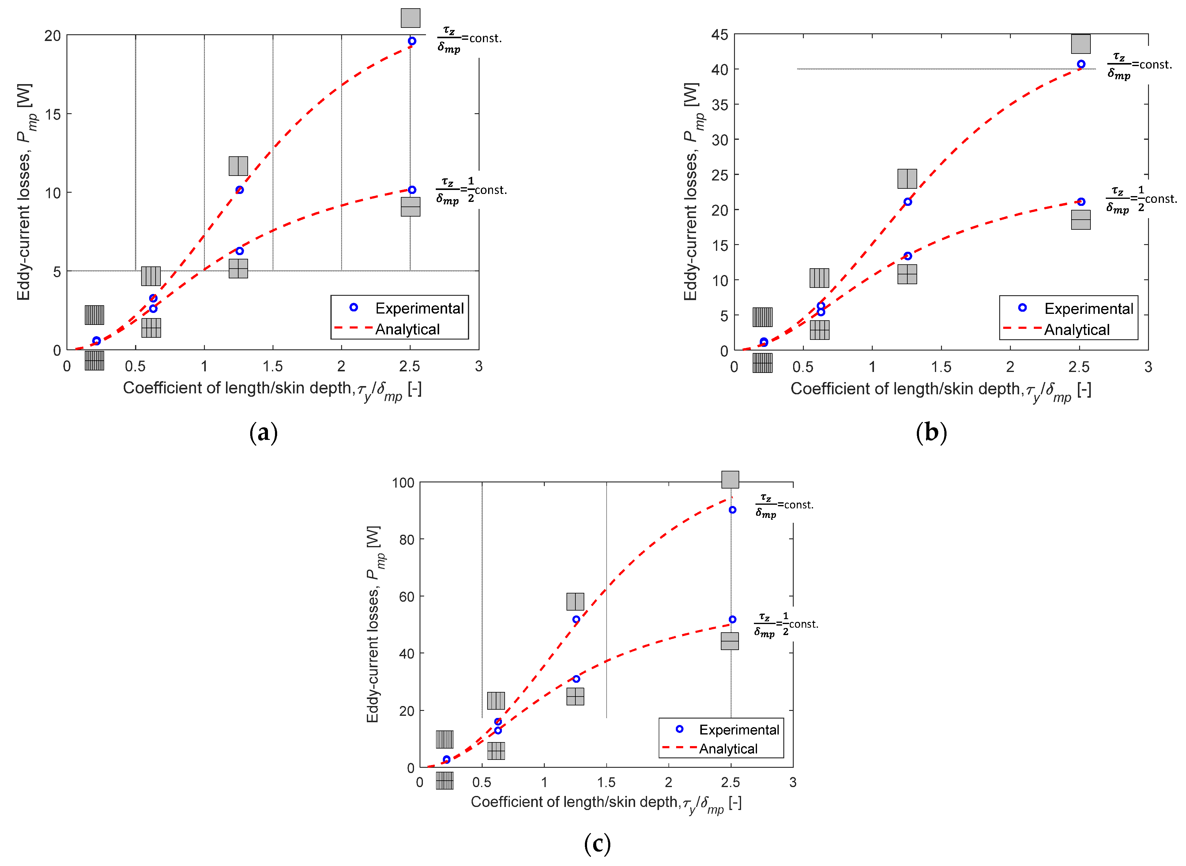
Coefficient of Length/Skin Depth Study: For this comparison analysis, $I$ = 3 A (viz., $V$ = 90 V). In order to study the segmentation influence on volumic eddy-current losses, they were plotted in relation to the coefficient of length/skin depth in both directions (such as ${\tau }_y/{\delta }_{mp}$ in the $y$-axis and ${\tau }_z/{\delta }_{mp}$ in the $z$-axis). In our study, the skin depth ${\delta }_{mp}$ = 16 mm.

Figure 22 shows $P_{mp}$ according to ${\tau }_y/{\delta }_{mp}$ and ${\tau }_z/{\delta }_{mp}$ for the various segmentations $\left\{N{s}_z,N{s}_y\right\}$ (Figure 5) and every thickness. The analytical results compared to the experimental measurements are consistent with a maximum error of less than 5% (viz., 4.67% for 4.67 W of difference for $P_{mp}=95$ W with $\left\{1,1\right\}$ and $h_{mp}=2$ mm).

Table 2. Various segmentations in both directions vs. cross-section and perimeter of a conductive segment and coefficient of length/skin depth.

$\left\{\mathit{N}{\mathit{s}}_{\mathit{z}},\mathit{N}{\mathit{s}}_{\mathit{y}}\right\}$		${\mathit{S}}_{\mathit{c}\mathit{s}}$ (mm2)	${\mathit{L}}_{\mathit{c}\mathit{s}}$ (mm)	${\mathit{\tau }}_{\mathit{y}}/{\mathit{\delta }}_{\mathit{m}\mathit{p}}$	${\mathit{\tau }}_{\mathit{z}}/{\mathit{\delta }}_{\mathit{m}\mathit{p}}$
{1,1}		1600	160	2.513	2.513
{1,2}		800	120	1.257	2.513
{1,4}		400	100	0.628	2.513
{1,10}		160	88	0.251	2.513
{2,1}		800	120	2.513	1.257
{2,2}		400	80	1.257	1.257
{2,4}		200	60	0.628	1.257
{2,10}		80	48	0.251	1.257

presents the various segmentations $\left\{N{s}_z,N{s}_y\right\}$ following the cross-section of a conductive segment $S_{cs}$, the perimeter of a conductive segment $L_{cs}$, ${\tau }_y/{\delta }_{mp}$, and ${\tau }_z/{\delta }_{mp}$. Firstly, it is interesting to note that $P_{mp}$ is the same for $\left\{1,2\right\}$ and $\left\{2,1\right\}$, $\forall h_{mp}$. Secondly, $P_{mp}$ decreases considerably when the ratios ${\tau }_y/{\delta }_{mp}$ and/or ${\tau }_z/{\delta }_{mp}$ are reduced, e.g., a loss reduction = $\approx$50% when ${\tau }_y/{\delta }_{mp}$ and/or ${\tau }_z/{\delta }_{mp}$ is divided by 2: $\left\{1,2\right\}$, $\left\{2,1\right\}$ and $\left\{2,2\right\}$ compared to $\left\{1,1\right\}$, $\forall h_{mp}$. It can also be seen that for a segmentation > 4 in the $y$-axis, the segmentation into 2 in the $z$-axis has an insignificant influence on the loss reduction (viz., $P_{mp}$ for $\left\{1,4\right\}$ # $P_{mp}$ for $\left\{4,2\right\}$ and $P_{mp}$ for $\left\{1,10\right\}$ $\cong$ $P_{mp}$ for $\left\{2,10\right\}$). Thirdly, for $\left\{1,4\right\}$ and $\left\{2,2\right\}$, it could be observed that $S_{cs}$ is identical, however, $P_{mp}$ is different (viz., $P_{mp}$ for $\left\{1,4\right\}$ < $P_{mp}$ for $\left\{2,2\right\}$). The segmentation $\left\{1,4\right\}$ is more efficient since it presents a ratio ${\tau }_y/{\delta }_{mp}$ = 0.628, while the segmentation $\left\{2,2\right\}$ has a ratio ${\tau }_y/{\delta }_{mp}$ = 1.257, $\forall h_{mp}$.

5. Conclusions

This paper conducts an electromagnetic analysis of the magnetic field generated by a U-shaped electromagnetic device with a flat mobile armature (or adjustable air gap) and a volumic eddy-current loss estimation in conductive massive parts.

The experimental device was presented in detail. It includes an electromagnet, aluminium conductive massive parts (aluminium: A-S5U3G) with(out) segmentation, and its instrumentation. The study on conductive massive parts was performed with a sinusoidal spatially uniform applied magnetic field at an excitation frequency of 50 Hz.

The spatial distribution of the magnetic field predicted by a 2D numerical model, under the FEMM software, has been compared to the experimental measurements. A good agreement between the experimental measurements and the numerical results has been achieved, with a mean percentage error (MPE) of less than 3%.

The accurate determination of the applied magnetic field has allowed an accurate eddy-current loss estimation in massive conductive parts. The losses were estimated from an analytical model, based on the Maxwell–Fourier method, and measured experimentally on (non-)segmented conductive massive parts. The analytically predicted eddy-current losses have been compared to the experimental results. The segmentation influence in both directions was studied. The comparison between the analytical and the experimental results allow the good accuracy to be confirmed. The maximal difference between experimental and analytical results is about 5 %, while the MPE is less than 2%.

Other frequencies (up to 600 Hz), time waveforms (e.g., six-step commutation, pulse-width modulation, etc.), geometrical shapes and materials (e.g., copper, brass, magnets, etc.) with different electrical conductivities [36] are a prospect for future study in order to explore the influence of segmentation further. Other prospects for future study are: (i) the volumic eddy-current loss distribution with a spatially non-uniform applied magnetic field, and (ii) the analytical and experimental validation of the eddy-currents reactance in conductive massive parts.

References

- Stoll, R.L. The Analysis of Eddy Currents; Clarendon Press: Oxfort, UK, 1974. [Google Scholar]
- Sikora, R.; Purczynski, J.; Lipinski, W.; Gramz, M. Use of variational methods to the eddy current calculation in thin conducting plates. IEEE Trans. Magn. 1978, 14, 383–385. [Google Scholar] [CrossRef]
- Dresner, L. Eddy current heating of irregularly shaped plates by slow ramped fields. OAK Ridge Natl. Lab. (ORNL) 1978, 6968, 1–44. [Google Scholar]
- Vansompel, H.; Yarantseva, A.; Sergeant, P.; Crevecoeur, G. An inverse thermal modeling approach for thermal parameter and loss identification in an axial flux permanent magnet machine. IEEE Trans. Ind. Electron. 2019, 66, 1727–1735. [Google Scholar] [CrossRef]
- Benlamine, R.; Dubas, F.; Randi, S.A.; Lhotellier, D.; Espanet, C. 3-D numerical hybrid method for PM eddy-current losses calculation: Application to axial-flux PMSMs. IEEE Trans. Magn. 2015, 51, 8106110. [Google Scholar] [CrossRef] [Green Version]
- Jassal, A.; Polinder, H.; Ferreira, J.A. Literature survey of eddy-current loss analysis in rotating electrical machines. IET Electr. Power Appl. 2012, 6, 743–752. [Google Scholar] [CrossRef]
- Dubas, F.; Rahideh, A. Two-dimensional analytical permanent-magnet eddy-current loss calculations in slotless PMSM equipped with surface-inset magnets. IEEE Trans. Magn. 2014, 50, 6300320. [Google Scholar] [CrossRef]
- Tessarolo, A. A survey of state-of-the-art methods to compute rotor eddy-current losses in synchronous permanent magnet machines. In Proceedings of the IEEE Workshop on Electrical Machines Design, Control and Diagnosis (WEMDCD), Nottingham, UK, 20–21 April 2017. [Google Scholar] [CrossRef]
- Ouamara, D.; Dubas, F. Permanent-magnet eddy-current losses: A global revision of calculation and analysis. Math. Comput. Appl. 2019, 24, 67. [Google Scholar] [CrossRef] [Green Version]
- Sirimanna, S.; Balachandran, T.; Haran, K.A. Review on magnet loss analysis, validation, design considerations, and reduction strategies in permanent magnet synchronous motors. Energies 2022, 15, 6116. [Google Scholar] [CrossRef]
- Jara, W.; Lindh, P.; Tapia, J.A.; Petrov, I.; Repo, A.K.; Pyrhönen, J. Rotor eddy-current losses reduction in an axial flux permanent-magnet machine. IEEE Trans. Ind. Electron. 2016, 63, 4729–4737. [Google Scholar] [CrossRef]
- De Paula Machado Bazzo, T.; Kölzer, J.F.; Carlson, R.; Wurtz, F.; Gerbaud, L. Multiphysics design optimization of a permanent magnet synchronous generator. IEEE Trans. Ind. Electron. 2017, 64, 9815–9823. [Google Scholar] [CrossRef]
- Zheng, J.; Zhao, W.; Ji, J.; Zhu, J.; Gu, C.; Zhu, S. Design to reduce rotor losses in fault-tolerant permanent-magnet machines. IEEE Trans. Ind. Electron. 2018, 65, 8476–8487. [Google Scholar] [CrossRef]
- Zhu, S.; Hu, Y.; Liu, C.; Wang, K. Iron loss and efficiency analysis of interior PM machines for electric vehicle applications. IEEE Trans. Ind. Electron. 2018, 65, 114–123. [Google Scholar] [CrossRef]
- Martinek, G.; Lanz, M.; Schneider, G.; Goll, D. Determination of AC losses in segmented rare earth permanent magnets. J. Appl. Phys. 2020, 128, 113902. [Google Scholar] [CrossRef]
- Amara, Y.; Wang, J.; Howe, D. Analytical prediction of eddy-current loss in modular tubular permanent-magnet machines. IEEE Trans. Energy Convers. 2005, 20, 761–770. [Google Scholar] [CrossRef]
- Yamazaki, K.; Abe, A. Loss investigation of interior permanent-magnet motors considering carrier harmonics and magnet eddy currents. IEEE Trans. Ind. Appl. 2009, 45, 659–665. [Google Scholar] [CrossRef]
- Huang, W.; Bettayeb, A.; Kaczmarek, R.; Vannier, J. Optimization of magnet segmentation for reduction of eddy-current losses in permanent magnet synchronous machine. IEEE Trans. Energy Convers. 2010, 25, 381–387. [Google Scholar] [CrossRef] [Green Version]
- Mirzaei, M.; Binder, A.; Funieru, B.; Susic, M. Analytical calculations of induced eddy currents losses in the magnets of surface mounted PM machines with consideration of circumferential and axial segmentation effects. IEEE Trans. Magn. 2012, 48, 4831–4841. [Google Scholar] [CrossRef]
- Mirzaei, M.; Binder, A.; Deak, C. 3D analysis of circumferential and axial segmentation effect on magnet eddy-current losses in permanent magnet synchronous machines with concentrated windings. In Proceedings of the XIX International Conference on Electrical Machines—ICEM 2010, Rome, Italy, 6–8 September 2010. [Google Scholar] [CrossRef]
- Balamurali, A.; Lai, C.; Mollaeian, A.; Loukanov, V.; Kar, N.C. Analytical investigation into magnet eddy current losses in interior permanent magnet motor using modified winding function theory accounting for pulsewidth modulation harmonics. IEEE Trans. Magn. 2016, 52, 8106805. [Google Scholar] [CrossRef]
- Nair, S.S.; Wang, J.; Chin, R.; Chen, L.; Sun, T. Analytical prediction of 3-D magnet eddy current losses in surface mounted PM machines accounting slotting effect. IEEE Trans. Energy Convers. 2017, 32, 414–423. [Google Scholar] [CrossRef]
- Aoyama, Y.; Miyata, K.; Ohashi, K. Simulations and experiments on eddy current in Nd-Fe-B magnet. IEEE Trans. Magn. 2005, 41, 3790–3792. [Google Scholar] [CrossRef]
- Yamazaki, K.; Shina, M.; Miwa, M.; Hagiwara, J. Investigation of eddy current loss in divided Nd-Fe-B sintered magnets for synchronous motors due to insulation resistance and frequency. IEEE Trans. Magn. 2008, 44, 4269–4272. [Google Scholar] [CrossRef]
- Yogal, N.; Lehrmann, C.; Henke, M. Permanent magnet eddy current loss measurement at higher frequency and temperature effects under ideal sinusoidal and non-sinusoidal external magnetic fields. In Proceedings of the IEEE Energy Conversion Congress and Exposition (ECCE), Vancouver, BC, Canada, 10–14 October 2021. [Google Scholar] [CrossRef]
- Deak, C.; Petrovic, L.; Binder, A.; Mirzaei, M.; Irimie, D.; Funieru, B. Calculation of eddy-current losses in permanent magnets of synchronous machines. In Proceedings of the IEEE International Symposium on Power Electronics, Electrical Drives, Automation and Motion (SPEEDAM), Ischia, Italy, 11–13 June 2008. [Google Scholar] [CrossRef]
- Plait, A.; Dubas, F. 2-D eddy-current losses model and experimental validation through thermal measurements. IEEE Trans. Instrum. Meas. 2022; under review. [Google Scholar]
- Fukuma, A.; Kanazawa, S.; Miyagi, D.; Takahashi, N. Investigation of AC loss of permanent magnet of SPM motor considering hysteresis and eddy-current losses. IEEE Trans. Magn. 2005, 41, 1964–1967. [Google Scholar] [CrossRef] [Green Version]
- Kanazawa, S.; Takahashi, N.; Kubo, T. Measurement and analysis of AC loss of NdFeB sintered magnet. Electr. Eng. Jpn. 2006, 154, 869–875. [Google Scholar] [CrossRef]
- Li, Y.; Jiang, B.; Zhang, C.; Liu, Y.; Gong, X. Eddy-current loss measurement of permanent magnetic material at different frequency. Int. J. Appl. Electromagn. Mech. 2019, 61, S13–S22. [Google Scholar] [CrossRef]
- Fratila, R.; Benabou, A.; Tounzi, A.; Mipo, J.C. A combined experimental and finite element analysis method for the estimation of eddy-current loss in NdFeB magnets. Sensors 2014, 14, 8505–8512. [Google Scholar] [CrossRef] [PubMed] [Green Version]
- Takahashi, N.; Shinagawa, H.; Miyagi, D.; Doi, Y.; Miyata, K. Analysis of eddy current losses of segmented Nd-Fe-B sintered magnets considering contact resistance. IEEE Trans. Magn. 2009, 45, 1234–1237. [Google Scholar] [CrossRef]
- Tong, W.; Hou, M.; Sun, L.; Wu, S. Analysis and experimental verification of segmented rotor structure on rotor eddy current loss of high-speed surface-mounted permanent magnet machine. In Proceedings of the IEEE International Magnetic Conference (INTERMAG), Lyon, France, 26–30 April 2021. [Google Scholar] [CrossRef]
- Meeker, D.C. Finite Element Method Magnetics Ver. 4.2. Available online: http://www.femm.info (accessed on 21 April 2019).
- Asensor Technology AB, Linear High Precision Analog Hall Sensors. Available online: https://www.asensor.eu (accessed on 8 November 2022).
- Plait, A.; Dubas, F. Electrical conductivity influence on eddy-current losses: Analytical study and experimental validation. In Proceedings of the IEEE International Conference on Electrical Machines and Systems (ICEMS), Gyeongju, Korea, 31 October–3 November 2021. (Best Paper Award from the IEEE ICEMS’22). [Google Scholar] [CrossRef]