
System Profit Improvement of a Thermal–Wind–CAES Hybrid System Considering Imbalance Cost in the Electricity Market
 ,
,  and
and
Abstract
:1. Introduction
- This work relates and differences between regulated and deregulated systems in presence of wind energy in the system.
- In a deregulated power context, a method is developed to examine the effects of the uncertainty of wind speed on the wind-incorporated power system. After the GENCOs and DISCOs adopted a power delivery bond (dependent on a wind speed estimate), if there was any discrepancy between the real and predicted wind speeds, ISO might reward or punish the GENCOs for their excess or deficiency in power supply. Therefore, GENCOs are working to close the power difference between real and predicted wind speed in order to avoid the negative impact of imbalance costs.
- The ESS is the only choice to alleviate this power shortfall. The energy storage systems in a competitive power market can mitigate the power difference and also minimize the burden on thermal power plants, so the financial profit can be exploited.
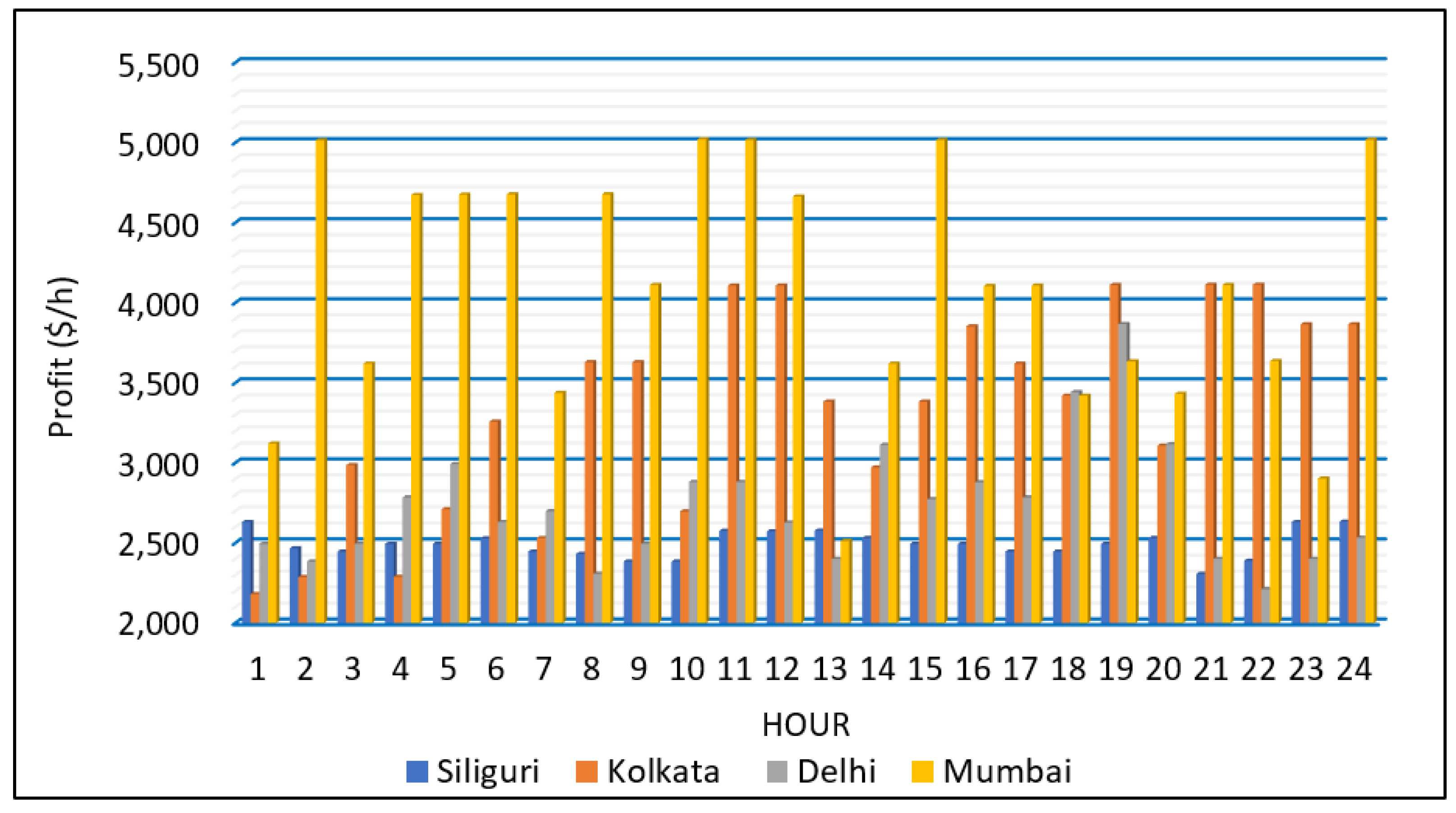
- The influence of system imbalance cost on the profit is deliberated here for four different locations in India based on the predicted and real wind speed for 24 h.
- A compressed air energy storage (CAES) system has been utilized here to diminish the damaging influences of imbalance costs in the thermal–wind–CAES hybrid system.
- Artificial bee colony algorithms (ABC) and moth flame optimization algorithms (MFO) have been put into action here to check the effectiveness of the proposed method along with sequential quadratic programming (SQP).
- The proportional studies of system risk before and after placement of the CAES system are also illustrated here with different optimization methodologies.
- The effect of imbalance cost has been assessed. The novelty of the work lies in the use of CAES which has been used to maximize the profit by minimizing the effect of imbalance cost which has not been done earlier.
2. Mathematical Modeling
2.1. Wind Speed Data
2.2. Wind Power and Wind Power Cost Calculation
2.3. Modeling of the CAES System
2.4. Locational Marginal Pricing (LMP)
2.5. Power Pool
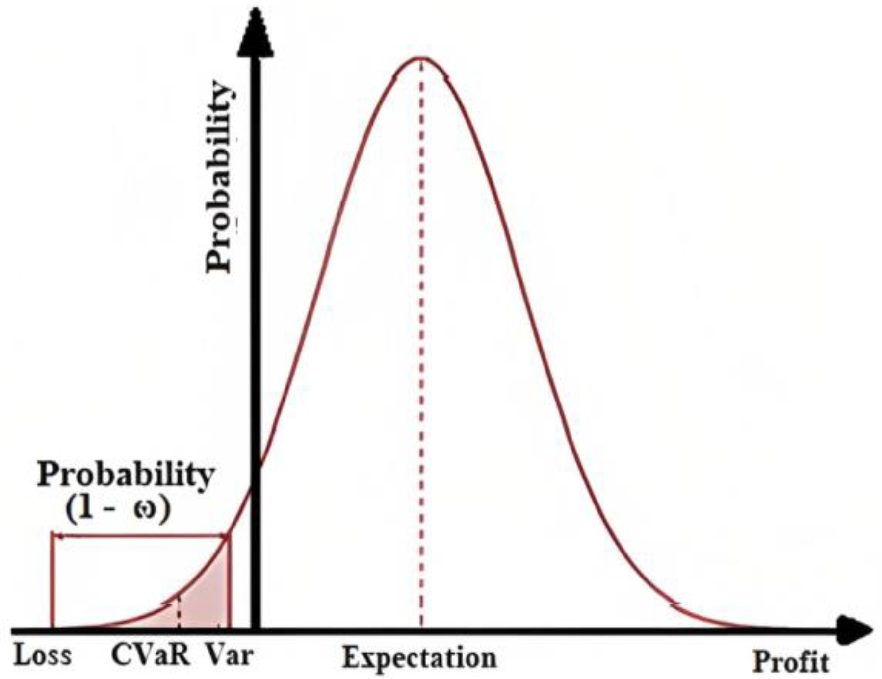
2.6. Value-at-Risk (VaR) and Conditional Value-at-Risk (CVaR)
3. Objective Function
- Second Part of the Objective Function:
3.1. Constraints
3.1.1. Constraints on Equality
- Equations for real power balance:
- Equations for power flow:
3.1.2. Constraints on Inequality
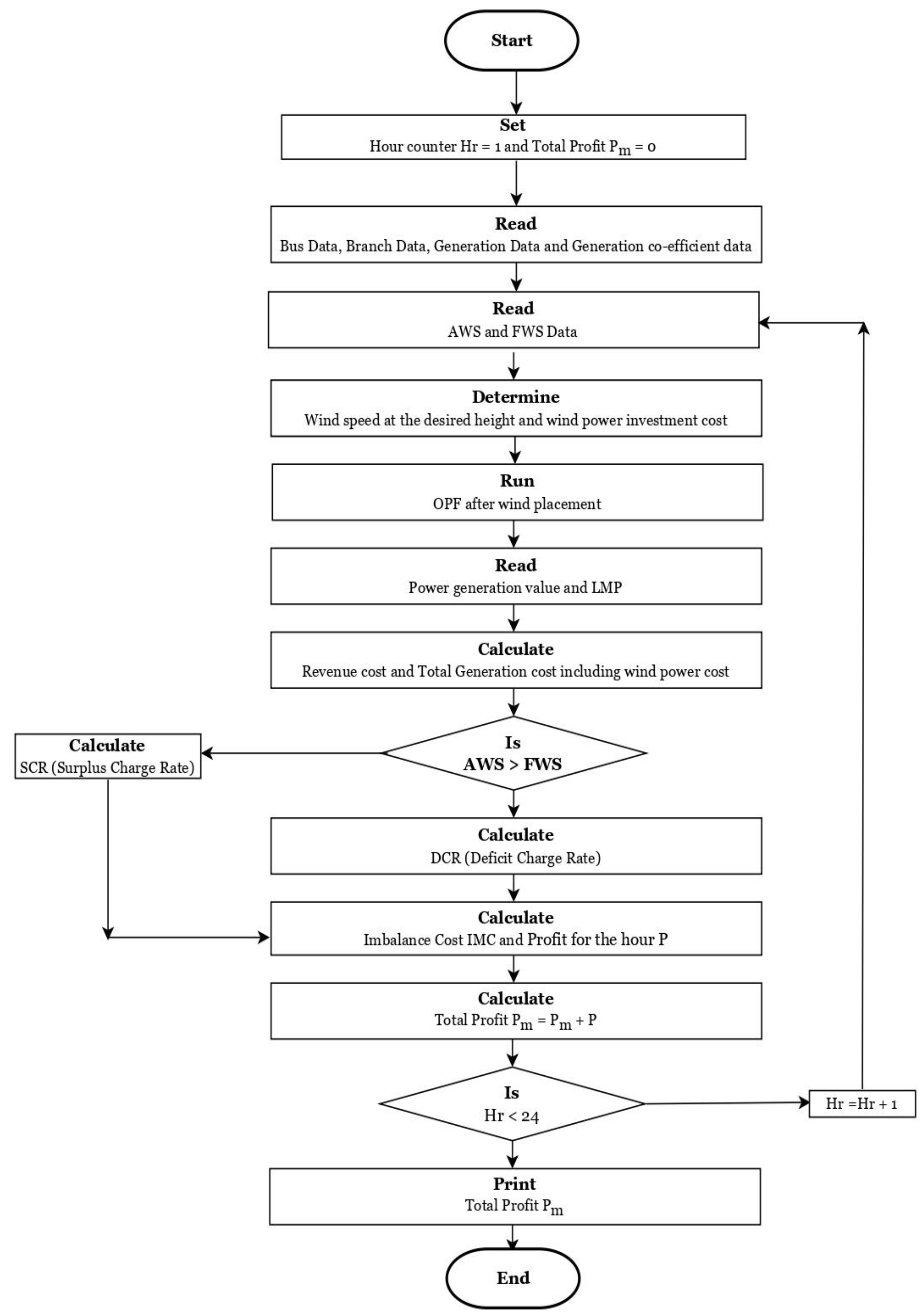
4. Proposed Method
5. Application of the Suggested Approach
- Regulated system;
- Deregulated system with single auction bidding;
- Deregulated system with double auction bidding.
- Case 1: Performance of the System for Single Auction Bidding Prior to Wind Installation
- Case 2: System Performance Prior to Wind Installation and When Double Auction Bidding Is Present
- Case 3: System Performance under Double Auction Bidding and Wind Positioning
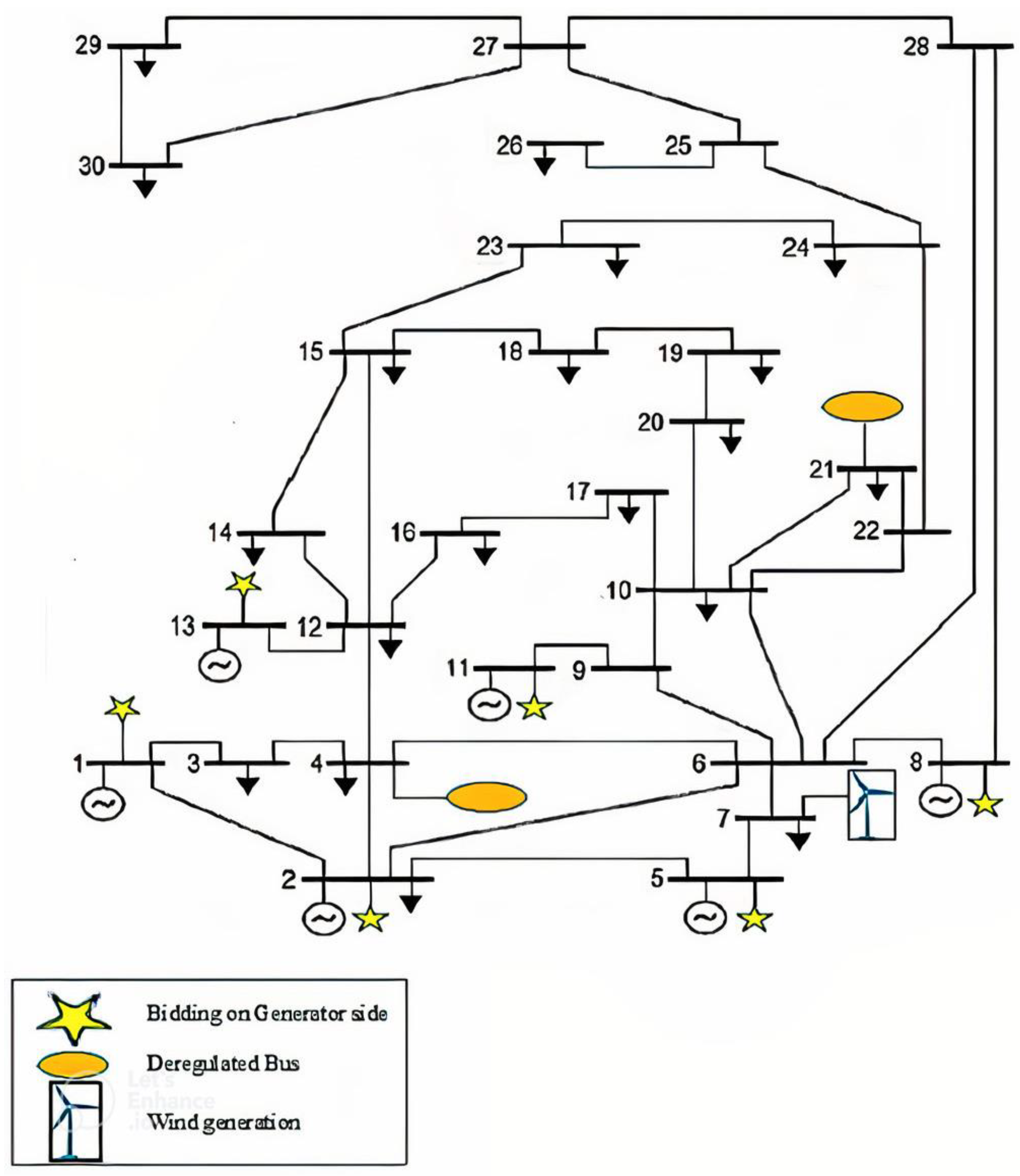
5.1. Profit Evaluation in a Modified IEEE 30-Bus System
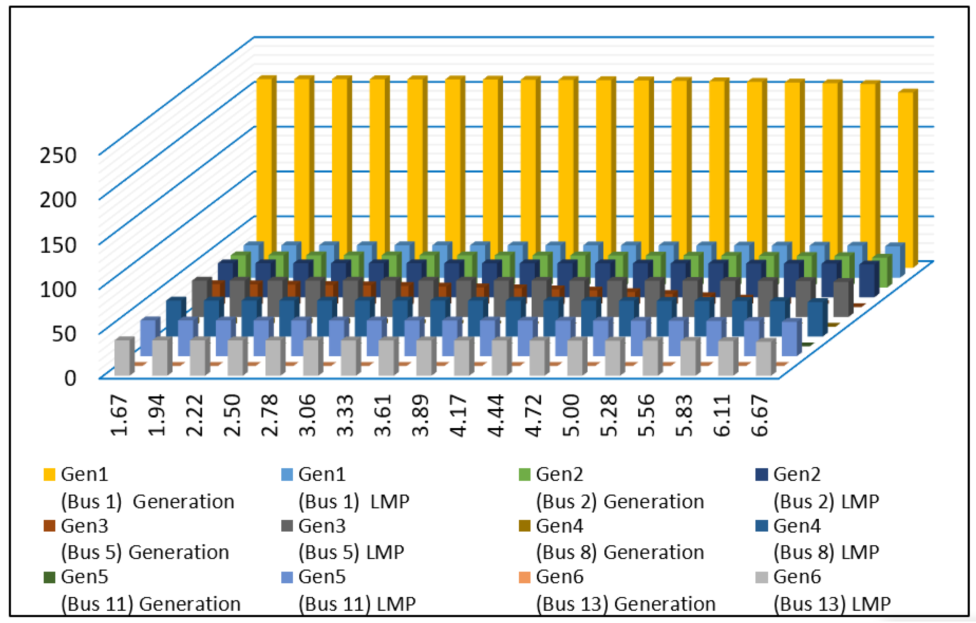
5.1.1. Generation and LMP Calculation
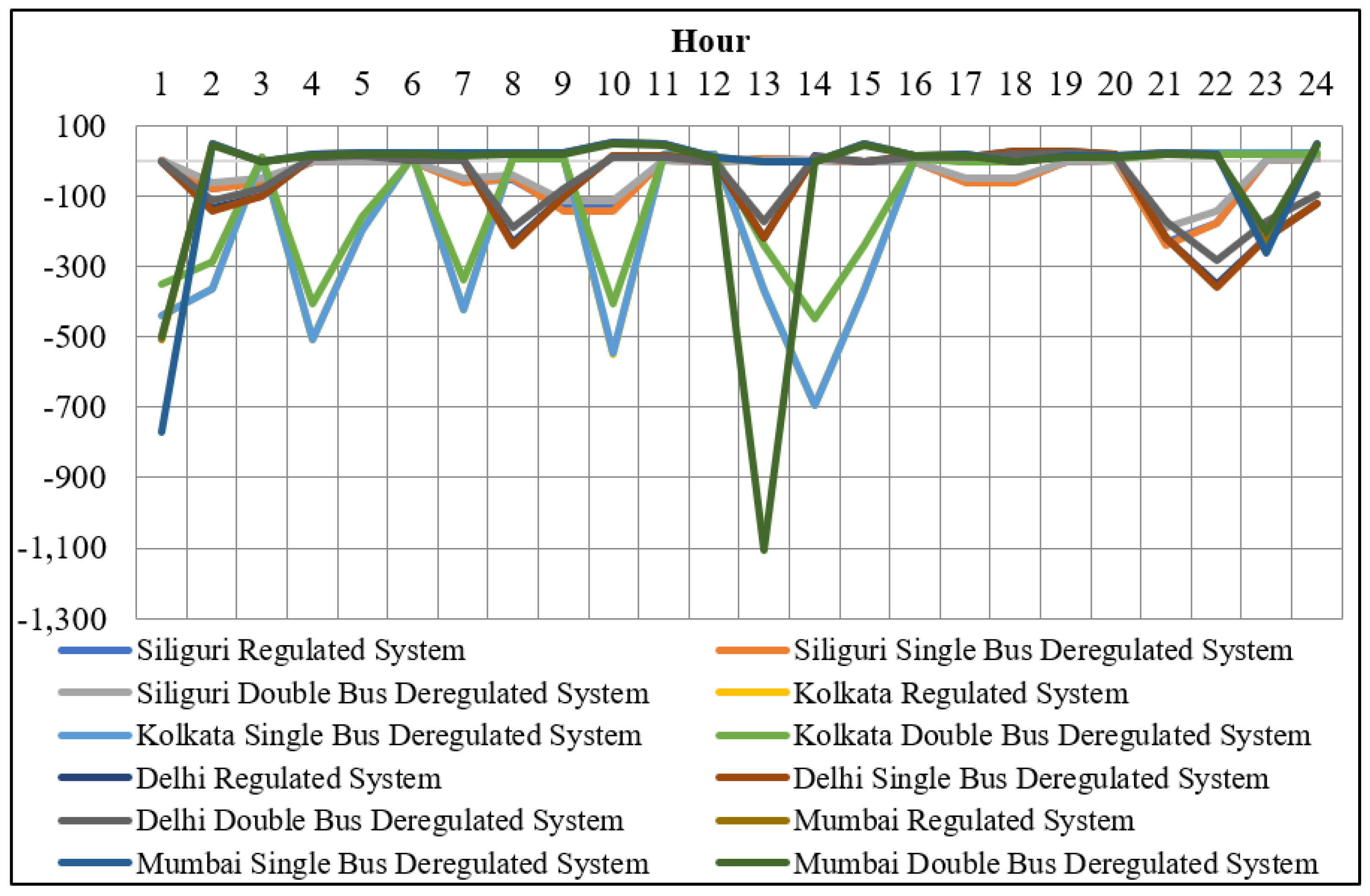
5.1.2. Calculation of Imbalance Cost
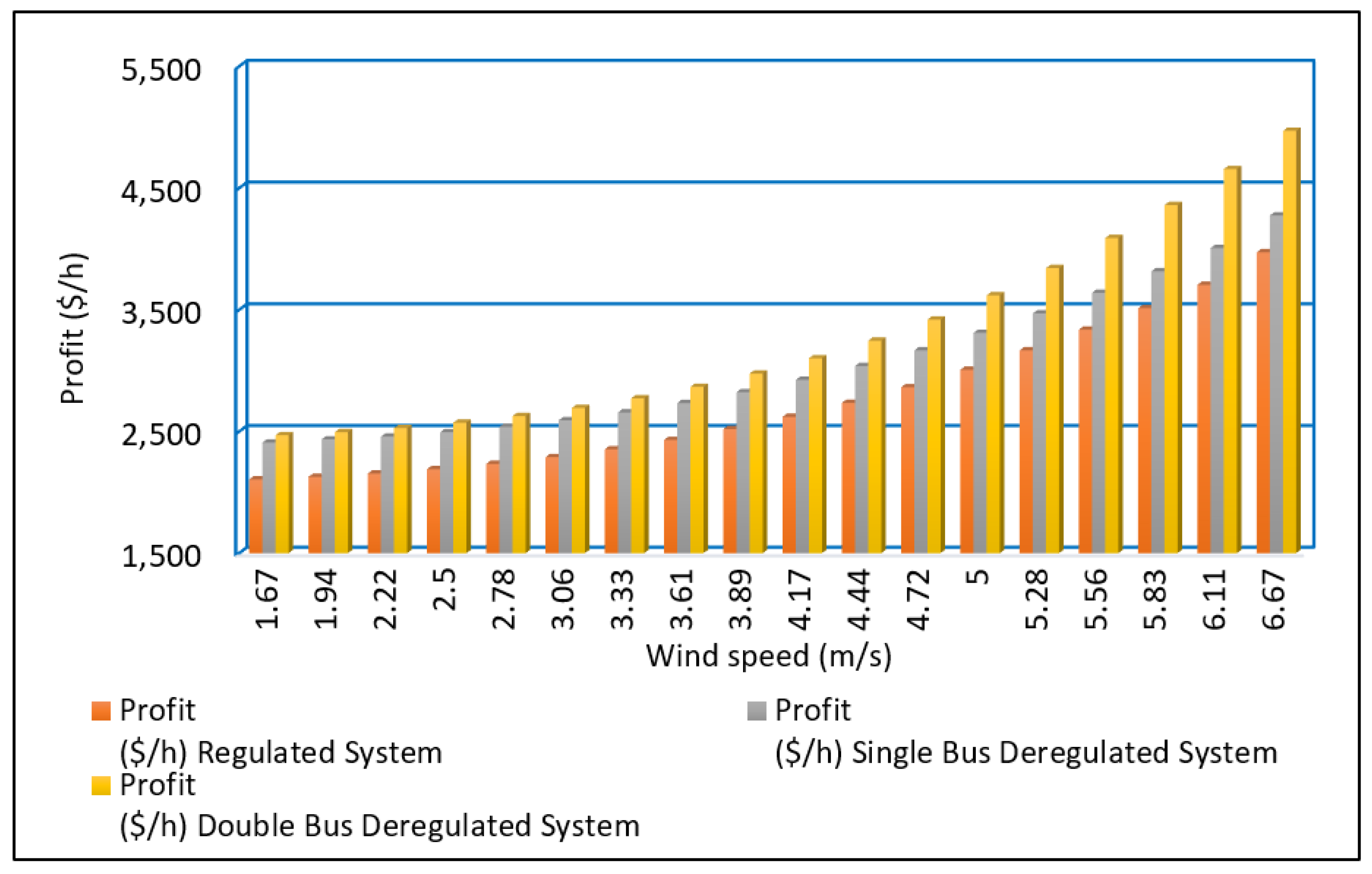
5.1.3. Profit Estimate for 24 h
5.2. Profit Comparison after WF Installation, Taking RWS and PWS into Consideration
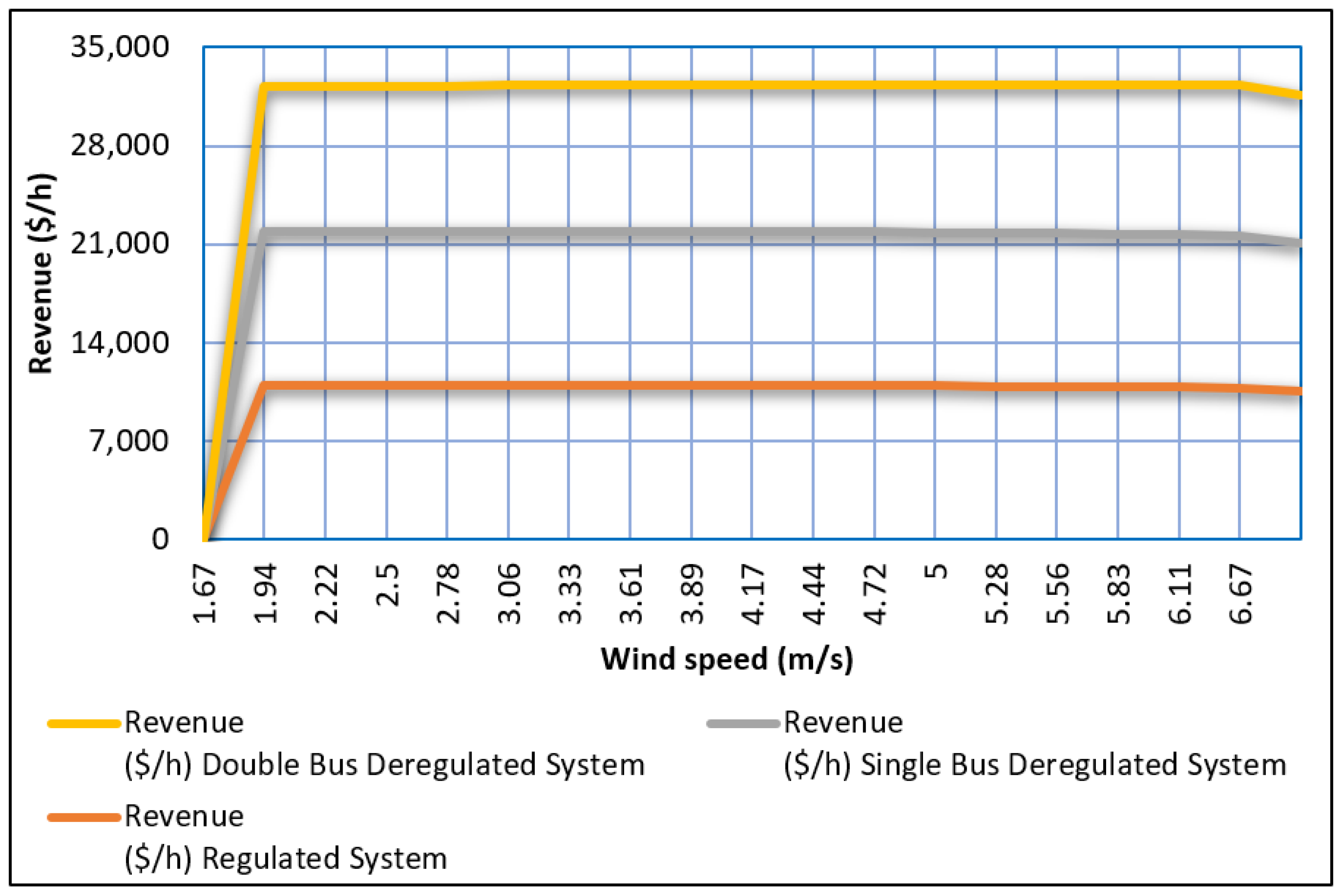
5.3. Revenue, Bus Voltage and Imbalance Cost after WF Placement
- Case 4: system performance with the placement of wind farm and CAES system
- Case 5: System risk Analysis with the placement of wind farm and CAES system
6. Conclusions
Author Contributions
Funding
Institutional Review Board Statement
Informed Consent Statement
Data Availability Statement
Conflicts of Interest
Abbreviations and Notations
| GENCOs | Generation Companies |
| TRANSCOs | Transmission Companies |
| DISCOs | Distribution Companies |
| APCDs | Air Pollution Control Devices |
| CAES | Compressed Air Energy Storage |
| CSP | Concentrated Solar Power |
| DAM | Day Ahead Markets |
| RFB | Redox Flow Battery |
| LMP | Locational Marginal Price |
| GWO | Grey Wolf Optimization |
| FA | Firefly Algorithm (FA) |
| PSO | Particle Swarm Optimization |
| MCP | Market Clearing Price |
| MCV | Market Clearing Volume |
| AGTO | Artificial Gorilla Troops Optimizer |
| MFO | Moth Flame Optimization |
| GSF | Generator Sensitivity Factor |
| ALO | Ant Lion Optimizer |
| ISO | Independent System Operator |
| ICR | Imbalance Charge Rate |
| SQP | Sequential Quadratic Programming |
| OPF | Optimal Power Flow |
| RWS | Real Wind Speed |
| PWS | Predicted Wind Speed |
| wind speed (at any height ‘’) | |
| reference wind speed | |
| Hellman’s co-efficient | |
| air density | |
| turbine’s swept area in | |
| efficiency (overall) of the wind plant | |
| power consumption of CAES (i.e., electric power of the compressor) while charging | |
| electric power generation of CAES (i.e., the electric power of the turbine) while discharging | |
| compressor efficiency | |
| efficiency of the turbine | |
| i-th generator’s cost curve at time t | |
| MCG | Marginal cost (generation) |
| MCL | Marginal cost (losses) |
| MCTC | Marginal cost (transmission congestion) |
| APGP | vector of the active power generation in the pool |
| APLP | vector of the active power demand in the pool |
| APGT | total active power generation vector |
| APLT | total active power demand vector |
| Tg | total number of generators |
| Td | total number of loads |
| Pm(t) | the m-th unit’s total profit at time ‘t’ |
| TRm(t) | total revenue |
| IMCm(t) | total imbalance cost |
| TGCm(t) | total generation cost |
| power generated with real wind speed at time ‘t’ at i-th generation bus | |
| power generated with predicted wind speed | |
| charge rate (surplus) at time ‘t’ | |
| charge rate (deficit) at time ‘t’ | |
| LMP at time ‘t’ at i-th bus | |
| Power generation cost of the thermal unit | |
| generated power at i-th generating unit | |
| wind power | |
| transmission loss | |
| demand in power | |
| overall system transmission lines count | |
| The line conductance between buses ‘i’ and ‘j’ | |
| magnitude and angle of voltage of bus ‘i’ | |
| magnitude and angle of voltage of bus ‘j’ | |
| real power injected into the system at the bus ‘i’ | |
| reactive power injected into the system at the bus ‘i’ | |
| bus ‘i’’s lower voltage limit | |
| bus ‘i’’s upper voltage limit | |
| lower angle limit corresponding to the voltage of bus ‘i’ | |
| upper angle limit corresponding to the voltage of bus ‘i’ | |
| actual line flow of line ‘l’ | |
| maximum line flow limit of Line ‘l’ | |
| lower real power limit of bus ‘I’ | |
| maximum real power limit of bus ‘I’ | |
| lower reactive power limit of bus ‘i’ | |
| maximum reactive power limit of bus ‘i’ |
References
- Gencer, B.; Larsen, E.R.; van Ackere, A. Understanding the coevolution of electricity markets and regulation. Energy Policy 2020, 143, 111585. [Google Scholar] [CrossRef]
- Shahidehpour, M.; Marwali, M. Introduction. In Maintenance Scheduling in Restructured Power Systems; The Springer International Series in Engineering and Computer Science; Springer: Boston, MA, USA, 2000. [Google Scholar] [CrossRef]
- AL Shaqsi, A.Z.; Sopian, K.; Al-Hinai, A. Review of energy storage services, applications, limitations, and benefits. Energy Rep. 2020, 6 (Suppl. S7), 288–306. [Google Scholar] [CrossRef]
- OECD Green Growth Studies, Energy. Available online: https://www.oecd.org/greengrowth/greening-energy/49157219.pdf (accessed on 6 August 2022).
- Kumar, M. Social, Economic, and Environmental Impacts of Renewable Energy Resources. In Wind Solar Hybrid Renewable Energy System; IntechOpen: London, UK, 2020; Available online: https://www.intechopen.com/chapters/70874 (accessed on 6 August 2022). [CrossRef] [Green Version]
- Bublitz, A.; Keles, D.; Zimmermann, F.; Fraunholz, C.; Fichtner, W. A survey on electricity market design: Insights from theory and real-world implementations of capacity remuneration mechanisms. Energy Econ. 2019, 80, 1059–1078, ISSN 0140-9883. [Google Scholar] [CrossRef]
- Razzaghi Asl, S. Re-powering the Nature-Intensive Systems: Insights From Linking Nature-Based Solutions and Energy Transition. Front. Sustain. Cities 2022, 4, 91. [Google Scholar] [CrossRef]
- Climate Impacts Energy. United States Environmental Protection Agency (EPA). Available online: https://19january2017snapshot.epa.gov/climate-impacts/climate-impacts-energy_html (accessed on 7 August 2022).
- Abdallah, L.; El-Shennawy, T. Reducing Carbon Dioxide Emissions from Electricity Sector Using Smart Electric Grid Applications. J. Eng. 2013, 2013, 845051. [Google Scholar] [CrossRef] [Green Version]
- Necoechea-Porras, P.; López, A.; Salazar-Elena, J. Deregulation in the Energy Sector and Its Economic Effects on the Power Sector: A Literature Review. Sustainability 2021, 13, 3429. [Google Scholar] [CrossRef]
- Das, C.K.; Bass, O.; Kothapalli, G.; Mahmoud, T.S.; Habibi, D. Overview of energy storage systems in distribution networks: Placement, sizing, operation, and power quality. Renew. Sustain. Energy Rev. 2018, 91, 1205–1230. [Google Scholar] [CrossRef]
- Energy Storage Important to Creating Affordable, Reliable, Deeply Decarbonized Electricity Systems. Available online: https://news.mit.edu/2022/energy-storage-important-creating-affordable-reliable-deeply-decarbonized-electricity-systems-0516 (accessed on 11 August 2022).
- Stephens, J.C. Energy Democracy: Redistributing Power to the People Through Renewable Transformation. Environ. Sci. Policy Sustain. Dev. 2019, 61, 4–13. [Google Scholar] [CrossRef]
- Ugurlu, U.; Tas, O.; Kaya, A.; Oksuz, I. The Financial Effect of the Electricity Price Forecasts’ Inaccuracy on a Hydro-Based Generation Company. Energies 2018, 11, 2093. [Google Scholar] [CrossRef] [PubMed] [Green Version]
- Liu, J.; Bo, R.; Wang, S.; Chen, H. Optimal scheduling for profit maximization of energy storage merchants considering market impact based on dynamic programming. Comput. Ind. Eng. 2021, 155, 107212. [Google Scholar] [CrossRef]
- The Economics of Grid-Scale Energy Storage in Wholesale Electricity Markets. Available online: https://climate.mit.edu/posts/economics-grid-scale-energy-storage-wholesale-electricity-markets#.YvDupD370d8.link (accessed on 8 August 2022).
- Rudkevich, A.; Duckworth, M.; Rosen, R. Modeling Electricity Pricing in a Deregulated Generation Industry: The Potential for Oligopoly Pricing in a Poolco. Energy J. 1998, 19. [Google Scholar] [CrossRef] [Green Version]
- Patil, G.S.; Mulla, A.; Dawn, S.; Ustun, T.S. Profit Maximization with Imbalance Cost Improvement by Solar PV-Battery Hybrid System in Deregulated Power Market. Energies 2022, 15, 5290. [Google Scholar] [CrossRef]
- Lan, P.; Han, D.; Zhang, R.; Xu, X.; Yan, Z. Optimal portfolio design of energy storage devices with financial and physical right market. Front. Energy 2022, 16, 95–104. [Google Scholar] [CrossRef]
- Siddiqui, A.S.; Sioshansi, R.; Conejo, A.J. Merchant Storage Investment in a Restructured Electricity Industry. Energy J. 2019, 40, 129–163. [Google Scholar] [CrossRef]
- Kumar, P.; Bharadwaj, S.K. Optimal Bidding Strategies and Profit Maximization for Micro Grid Combinations in Electric Energy Market in Indian Restructured Environment. Int. J. Adv. Res. Eng. Technol. 2020, 11, 931–949. Available online: https://ssrn.com/abstract=3658341 (accessed on 22 July 2020).
- Chen, W.; Tian, Y.; Zheng, K.; Wan, N. Influences of mechanisms on investment in renewable energy storage equipment. Environ. Dev. Sustain. 2022. [Google Scholar] [CrossRef]
- Murphy, C.; Schleifer, A.; Eurek, K. A taxonomy of systems that combine utility-scale renewable energy and energy storage technologies. Renew. Sustain. Energy Rev. 2021, 139, 110711. [Google Scholar] [CrossRef]
- Li, K.; Cursio, J.D.; Sun, Y.; Zhu, Z. Determinants of price fluctuations in the electricity market: A study with PCA and NARDL models. Econ. Res. 2019, 32, 2404–2421. [Google Scholar] [CrossRef] [Green Version]
- Zhang, M.; Chen, J.; Yang, Z.; Peng, K.; Zhao, Y.; Zhang, X. Stochastic day-ahead scheduling of irrigation system integrated agricultural microgrid with pumped storage and uncertain wind power. Energy 2021, 237, 121638. [Google Scholar] [CrossRef]
- Gilvaei, M.N.; Imani, M.H.; Ghadi, M.J.; Li, L.; Golrang, A. Profit-Based Unit Commitment for a GENCO Equipped with Compressed Air Energy Storage and Concentrating Solar Power Units. Energies 2021, 14, 576. [Google Scholar] [CrossRef]
- Selvaraju, R.K.; Somaskandan, G. Impact of energy storage units on load frequency control of deregulated power systems. Energy 2016, 97, 214–228. [Google Scholar] [CrossRef]
- Das, S.S.; Das, A.; Dawn, S.; Gope, S.; Ustun, T.S. A Joint Scheduling Strategy for Wind and Solar Photovoltaic Systems to Grasp Imbalance Cost in Competitive Market. Sustainability 2022, 14, 5005. [Google Scholar] [CrossRef]
- Yu, Q.; Tian, L.; Li, X.; Tan, X. Compressed Air Energy Storage Capacity Configuration and Economic Evaluation Considering the Uncertainty of Wind Energy. Energies 2022, 15, 4637. [Google Scholar] [CrossRef]
- Eladl, A.; Kaddah, S.; Haikal, E. Optimal generation rescheduling for congestion management, LMP enhancement and social welfare maximization. In Proceedings of the 2017 Nineteenth International Middle East Power Systems Conference (MEPCON), Cairo, Egypt, 19–21 December 2017; pp. 1190–1194. [Google Scholar] [CrossRef]
- Farzana, D.F.; Mahadevan, K. Performance comparison using firefly and PSO algorithms on congestion management of deregulated power market involving renewable energy sources. Soft Comput. 2020, 24, 1473–1482. [Google Scholar] [CrossRef]
- Gautam, A.; Sharma, P.; Kumar, Y. Mitigating congestion by optimal rescheduling of generators applying hybrid PSO–GWO in deregulated environment. SN Appl. Sci. 2021, 3, 69. [Google Scholar] [CrossRef]
- Özcan, M.; Keysan, O.; Satır, B. Optimum bidding strategy for wind and solar power plants in day-ahead electricity market. Energy Syst. 2021, 12, 955–987. [Google Scholar] [CrossRef]
- Kumar, K.K.P.; Soren, N.; Latif, A.; Das, D.C.; Hussain, S.M.S.; Al-Durra, A.; Ustun, T.S. Day-Ahead DSM-Integrated Hybrid-Power-Management-Incorporated CEED of Solar Thermal/Wind/Wave/BESS System Using HFPSO. Sustainability 2022, 14, 1169. [Google Scholar] [CrossRef]
- Singh, N.K.; Koley, C.; Gope, S.; Dawn, S.; Ustun, T.S. An Economic Risk Analysis in Wind and Pumped Hydro Energy Storage Integrated Power System Using Meta-Heuristic Algorithm. Sustainability 2021, 13, 13542. [Google Scholar] [CrossRef]
- Patil, G.S.; Mulla, A.; Ustun, T.S. Impact of Wind Farm Integration on LMP in Deregulated Energy Markets. Sustainability 2022, 14, 4354. [Google Scholar] [CrossRef]
- Dawn, S.; Gope, S.; Das, S.S.; Ustun, T.S. Social Welfare Maximization of Competitive Congested Power Market Considering Wind Farm and Pumped Hydroelectric Storage System. Electronics 2021, 10, 2611. [Google Scholar] [CrossRef]
- Gope, S.; Dawn, S.; Das, S.S.; Galiveeti, H.R. Wind farm integrated restructured electricity market analysis using Ant Lion optimizer algorithm. Energy Sources Part A Recovery Util. Environ. Eff. 2021. [Google Scholar] [CrossRef]
- India Meteorological Department, Ministry of Earth Sciences, Government of India. AWS Lab, Pune. Available online: http://www.imd.gov.in/Welcome%20To%20IMD/Welcome.phpandhttp://www.imdaws.com/ViewAwsData.aspx (accessed on 10 July 2022).
- Database: World Temperatures-Weather around the World. Available online: www.timeanddate.com/weather (accessed on 12 July 2022).
- Dawn, S.; Tiwari, P.K.; Goswami, A.K. An approach for efficient assessment of the performance of double auction competitive power market under variable imbalance cost due to high uncertain wind penetration. Renew. Energy 2017, 108, 230–243. [Google Scholar] [CrossRef]
- Morthorst, P.E. Wind Energy—The Facts: Costs & Prices; RISO National Laboratory: Roskilde, Denmark, 2010; Volume 2, pp. 94–110. [Google Scholar]
- Dawn, S.; Tiwari, P.K. Improvement of economic profit by optimal allocation of TCSC & UPFC with wind power generators in double auction competitive power market. Int. J. Electr. Power Energy Syst. 2016, 80, 190–201. [Google Scholar] [CrossRef]
- Basu, J.B.; Dawn, S.; Saha, P.K.; Chakraborty, M.R.; Ustun, T.S. Economic Enhancement of Wind–Thermal–Hydro System Considering Imbalance Cost in Deregulated Power Market. Sustainability 2022, 14, 15604. [Google Scholar] [CrossRef]
- Tiwari, P.K.; Sood, Y.R. An Efficient Approach for Optimal Allocation and Parameters Determination of TCSC With Investment Cost Recovery Under Competitive Power Market. IEEE Trans. Power Syst. 2013, 28, 2475–2484. [Google Scholar] [CrossRef]
- Das, A.; Dawn, S.; Gope, S.; Ustun, T.S. A Risk Curtailment Strategy for Solar PV-Battery Integrated Competitive Power System. Electronics 2022, 11, 1251. [Google Scholar] [CrossRef]


| Hour | Siliguri | Kolkata | Mumbai | Delhi | ||||
|---|---|---|---|---|---|---|---|---|
| PWS | RWS | PWS | RWS | PWS | RWS | PWS | RWS | |
| 1. | 2.50 | 2.78 | 3.33 | 2.22 | 5.56 | 5.00 | 1.94 | 1.94 |
| 2. | 2.50 | 2.22 | 3.33 | 2.50 | 5.28 | 6.67 | 2.50 | 1.94 |
| 3. | 2.22 | 1.94 | 3.33 | 3.89 | 5.00 | 5.00 | 2.78 | 2.50 |
| 4. | 1.94 | 1.94 | 3.89 | 3.06 | 4.72 | 6.11 | 2.50 | 3.33 |
| 5. | 1.94 | 1.94 | 3.89 | 3.61 | 4.17 | 6.11 | 2.50 | 3.89 |
| 6. | 2.22 | 2.22 | 3.89 | 4.44 | 3.61 | 6.11 | 2.50 | 2.78 |
| 7. | 2.22 | 1.94 | 4.17 | 3.61 | 3.61 | 4.72 | 2.78 | 3.06 |
| 8. | 1.94 | 1.67 | 4.72 | 5.00 | 3.61 | 6.11 | 2.78 | 1.94 |
| 9. | 2.50 | 1.94 | 4.72 | 5.00 | 3.89 | 5.56 | 2.78 | 2.50 |
| 10. | 2.50 | 1.94 | 4.72 | 4.17 | 4.17 | 6.67 | 2.50 | 3.61 |
| 11. | 2.22 | 2.50 | 4.72 | 5.56 | 5.00 | 6.67 | 2.50 | 3.61 |
| 12. | 2.50 | 2.50 | 4.72 | 5.56 | 5.83 | 6.11 | 2.78 | 2.78 |
| 13. | 1.94 | 2.50 | 5.28 | 5.00 | 6.11 | 5.00 | 3.06 | 2.50 |
| 14. | 1.94 | 2.22 | 5.28 | 4.72 | 5.00 | 5.00 | 3.61 | 4.17 |
| 15. | 1.94 | 1.94 | 5.28 | 5.00 | 5.00 | 6.67 | 3.33 | 3.33 |
| 16. | 1.94 | 1.94 | 5.00 | 5.28 | 5.00 | 5.56 | 2.78 | 3.61 |
| 17. | 2.22 | 1.94 | 5.00 | 5.00 | 4.72 | 5.56 | 2.50 | 3.33 |
| 18. | 2.22 | 1.94 | 4.72 | 4.72 | 4.72 | 4.72 | 2.50 | 4.72 |
| 19. | 1.94 | 1.94 | 4.17 | 5.56 | 4.44 | 5.00 | 2.78 | 5.28 |
| 20. | 1.94 | 2.22 | 3.89 | 4.17 | 4.17 | 4.72 | 3.06 | 4.17 |
| 21. | 2.78 | 1.94 | 3.61 | 5.56 | 4.17 | 5.56 | 3.06 | 2.50 |
| 22. | 2.78 | 2.22 | 3.61 | 5.56 | 4.17 | 5.00 | 3.06 | 1.94 |
| 23. | 2.50 | 2.78 | 3.61 | 5.28 | 4.44 | 4.17 | 3.06 | 2.50 |
| 24. | 2.22 | 2.78 | 3.61 | 5.28 | 4.72 | 6.67 | 3.06 | 2.78 |
| Sl. No. | Wind Speed at 10 m (m/s) | Wind Speed at 120 m (m/s) | Wind Power with 50 Turbines (MW) | Wind Gen Cost with 50 Turbines ($/h) |
|---|---|---|---|---|
| 1 | 1.67 | 2.38 | 1.01 | 3.799 |
| 2 | 1.94 | 2.77 | 1.61 | 6.032 |
| 3 | 2.22 | 3.17 | 2.40 | 9.004 |
| 4 | 2.50 | 3.57 | 3.42 | 12.820 |
| 5 | 2.78 | 3.96 | 4.69 | 17.586 |
| 6 | 3.06 | 4.36 | 6.24 | 23.407 |
| 7 | 3.33 | 4.75 | 8.10 | 30.389 |
| 8 | 3.61 | 5.15 | 10.30 | 38.637 |
| 9 | 3.89 | 5.55 | 12.87 | 48.257 |
| 10 | 4.17 | 5.94 | 15.83 | 59.353 |
| 11 | 4.44 | 6.34 | 19.21 | 72.033 |
| 12 | 4.72 | 6.73 | 23.04 | 86.401 |
| 13 | 5.00 | 7.13 | 27.35 | 102.563 |
| 14 | 5.28 | 7.53 | 32.17 | 120.624 |
| 15 | 5.56 | 7.92 | 37.52 | 140.690 |
| 16 | 5.83 | 8.32 | 43.43 | 162.866 |
| 17 | 6.11 | 8.72 | 49.94 | 187.258 |
| 18 | 6.67 | 9.51 | 64.83 | 243.112 |
| Generation (MW) | LMP ($/MW) | Generation Cost ($/h) | Revenue Cost ($/h) | |
|---|---|---|---|---|
| Gen 1 (Bus 1) | 212.25 | 36.414 | 8602.87 | 10,996.74 |
| Gen 2 (Bus 2) | 36.23 | 38.115 | ||
| Gen 3 (Bus 5) | 29.36 | 40.587 | ||
| Gen 4 (Bus 8) | 12.93 | 40.259 | ||
| Gen 5 (Bus 11) | 4.36 | 40.087 | ||
| Gen 6 (Bus 13) | 0 | 39.651 |
| Generation (MW) | LMP ($/MW) | Generation Cost ($/h) | Revenue Cost ($/h) | |
|---|---|---|---|---|
| Gen 1 (Bus 1) | 210.86 | 36.207 | 7896.03 | 10,321.36 |
| Gen 2 (Bus 2) | 36 | 37.998 | ||
| Gen 3 (Bus 5) | 26.04 | 40.521 | ||
| Gen 4 (Bus 8) | 6.57 | 40.131 | ||
| Gen 5 (Bus 11) | 0 | 39.841 | ||
| Gen 6 (Bus 13) | 0 | 39.528 |
| Sl. No. | Wind Speed (m/s) | Revenue ($/h) | Generation Cost ($/h) | Profit ($/h) |
|---|---|---|---|---|
| 1. | 1.67 | 10,327.831 | 7859.009 | 2468.823 |
| 2. | 1.94 | 10,330.800 | 7837.002 | 2493.797 |
| 3. | 2.22 | 10,335.824 | 7808.064 | 2527.760 |
| 4. | 2.50 | 10,342.368 | 7770.710 | 2571.657 |
| 5. | 2.78 | 10,350.565 | 7724.246 | 2626.319 |
| 6. | 3.06 | 10,360.481 | 7667.597 | 2692.884 |
| 7. | 3.33 | 10,372.007 | 7599.679 | 2772.328 |
| 8. | 3.61 | 10,385.406 | 7519.427 | 2865.979 |
| 9. | 3.89 | 10,400.933 | 7425.817 | 2975.116 |
| 10. | 4.17 | 10,418.721 | 7318.183 | 3100.538 |
| 11. | 4.44 | 10,441.601 | 7195.533 | 3246.068 |
| 12. | 4.72 | 10,475.785 | 7056.871 | 3418.914 |
| 13. | 5.00 | 10,520.177 | 6901.293 | 3618.885 |
| 14. | 5.28 | 10,570.406 | 6727.894 | 3842.512 |
| 15. | 5.56 | 10,625.454 | 6536.160 | 4089.294 |
| 16. | 5.83 | 10,685.383 | 6325.256 | 4360.127 |
| 17. | 6.11 | 10,749.535 | 6093.968 | 4655.567 |
| 18. | 6.67 | 10,542.761 | 5573.142 | 4969.620 |
| Wind Speed (m/s) | Gen1 (Bus 1) | Gen2 (Bus 2) | Gen3 (Bus 5) | Gen4 (Bus 8) | Gen5 (Bus 11) | Gen6 (Bus 13) | ||||||
|---|---|---|---|---|---|---|---|---|---|---|---|---|
| Generation ($) | LMP ($/MWh) | Generation ($) | LMP ($/MWh) | Generation ($) | LMP ($/MWh) | Generation ($) | LMP ($/MWh) | Generation ($) | LMP ($/MWh) | Generation ($) | LMP ($/MWh) | |
| 1.67 | 210.78 | 36.20 | 35.98 | 37.99 | 25.65 | 40.51 | 6.24 | 40.13 | 0.00 | 39.88 | 0.00 | 39.52 |
| 1.94 | 210.73 | 36.20 | 35.97 | 37.99 | 25.41 | 40.51 | 6.04 | 40.12 | 0.00 | 39.83 | 0.00 | 39.51 |
| 2.22 | 210.66 | 36.19 | 35.96 | 37.98 | 25.11 | 40.50 | 5.78 | 40.12 | 0.00 | 39.82 | 0.00 | 39.51 |
| 2.50 | 210.58 | 36.19 | 35.95 | 37.97 | 24.71 | 40.49 | 5.45 | 40.11 | 0.00 | 39.81 | 0.00 | 39.50 |
| 2.78 | 210.48 | 36.18 | 35.93 | 37.97 | 24.22 | 40.48 | 5.04 | 40.10 | 0.00 | 39.80 | 0.00 | 39.48 |
| 3.06 | 210.36 | 36.17 | 35.91 | 37.95 | 23.62 | 40.47 | 4.53 | 40.09 | 0.00 | 39.79 | 0.00 | 39.47 |
| 3.33 | 210.21 | 36.16 | 35.88 | 37.94 | 22.90 | 40.46 | 3.93 | 40.08 | 0.00 | 39.78 | 0.00 | 39.45 |
| 3.61 | 210.03 | 36.14 | 35.85 | 37.92 | 22.05 | 40.44 | 3.21 | 40.06 | 0.00 | 39.76 | 0.00 | 39.43 |
| 3.89 | 209.82 | 36.13 | 35.81 | 37.91 | 21.06 | 40.42 | 2.38 | 40.05 | 0.00 | 39.74 | 0.00 | 39.41 |
| 4.17 | 209.58 | 36.11 | 35.77 | 37.88 | 19.91 | 40.40 | 1.43 | 40.03 | 0.00 | 39.72 | 0.00 | 39.38 |
| 4.44 | 209.28 | 36.09 | 35.72 | 37.86 | 18.55 | 40.37 | 0.50 | 40.00 | 0.00 | 39.69 | 0.00 | 39.34 |
| 4.72 | 208.85 | 36.05 | 35.64 | 37.82 | 16.78 | 40.34 | 0.05 | 39.95 | 0.00 | 39.64 | 0.00 | 39.29 |
| 5.00 | 208.29 | 36.01 | 35.54 | 37.77 | 14.62 | 40.29 | 0.00 | 39.89 | 0.00 | 39.58 | 0.00 | 39.22 |
| 5.28 | 207.66 | 35.96 | 35.43 | 37.72 | 12.19 | 40.24 | 0.00 | 39.81 | 0.00 | 39.52 | 0.00 | 39.14 |
| 5.56 | 206.96 | 35.91 | 35.31 | 37.66 | 9.50 | 40.19 | 0.00 | 39.73 | 0.00 | 39.45 | 0.00 | 39.06 |
| 5.83 | 206.18 | 35.85 | 35.18 | 37.59 | 6.54 | 40.13 | 0.00 | 39.64 | 0.00 | 39.37 | 0.00 | 38.96 |
| 6.11 | 205.33 | 35.78 | 35.03 | 37.51 | 3.28 | 40.07 | 0.00 | 39.53 | 0.00 | 39.28 | 0.00 | 38.86 |
| 6.67 | 195.70 | 35.04 | 33.32 | 36.66 | 0.00 | 39.05 | 0.00 | 38.51 | 0.00 | 38.27 | 0.00 | 37.88 |
| Hour | Siliguri | Kolkata | Delhi | Mumbai |
|---|---|---|---|---|
| 1 | 3.749 | −347.793 | 0.000 | −499.464 |
| 2 | −62.157 | −285.583 | −110.611 | 44.064 |
| 3 | −48.445 | 10.235 | −77.263 | 0.000 |
| 4 | 0.000 | −404.948 | 11.055 | 16.452 |
| 5 | 0.000 | −156.554 | 16.314 | 19.067 |
| 6 | 0.000 | 10.471 | 3.749 | 20.674 |
| 7 | −48.445 | −336.597 | 4.471 | 17.305 |
| 8 | −37.882 | 8.988 | −187.899 | 20.674 |
| 9 | −110.611 | 8.988 | −77.263 | 21.276 |
| 10 | −110.611 | −404.641 | 14.034 | 50.203 |
| 11 | 3.073 | 17.262 | 14.034 | 46.100 |
| 12 | 0.000 | 17.262 | 0.000 | 6.860 |
| 13 | 5.225 | −237.026 | −171.985 | −1107.252 |
| 14 | 2.433 | −448.376 | 10.382 | 0.000 |
| 15 | 0.000 | −237.026 | 0.000 | 46.100 |
| 16 | 0.000 | 9.463 | 12.169 | 14.258 |
| 17 | −48.445 | 0.000 | 11.055 | 17.262 |
| 18 | −48.445 | 0.000 | 22.040 | 0.000 |
| 19 | 0.000 | 20.387 | 23.969 | 14.040 |
| 20 | 2.433 | 6.541 | 15.208 | 12.076 |
| 21 | −187.899 | 22.039 | −171.985 | 20.387 |
| 22 | −139.435 | 22.039 | −282.652 | 16.939 |
| 23 | 3.749 | 22.006 | −171.985 | −199.299 |
| 24 | 6.372 | 22.006 | −94.701 | 47.895 |
| Hour | Siliguri | Kolkata | Delhi | Mumbai |
|---|---|---|---|---|
| 1 | 2630.068 | 2179.967 | 2493.797 | 3119.421 |
| 2 | 2465.603 | 2286.074 | 2383.187 | 5013.683 |
| 3 | 2445.352 | 2985.351 | 2494.394 | 3618.885 |
| 4 | 2493.797 | 2287.935 | 2783.383 | 4672.018 |
| 5 | 2493.797 | 2709.425 | 2991.430 | 4674.634 |
| 6 | 2527.760 | 3256.539 | 2630.068 | 4676.241 |
| 7 | 2445.352 | 2529.382 | 2697.354 | 3436.219 |
| 8 | 2430.940 | 3627.873 | 2305.898 | 4676.241 |
| 9 | 2383.187 | 3627.873 | 2494.394 | 4110.570 |
| 10 | 2383.187 | 2695.897 | 2880.013 | 5019.823 |
| 11 | 2574.730 | 4106.556 | 2880.013 | 5015.720 |
| 12 | 2571.657 | 4106.556 | 2626.319 | 4662.426 |
| 13 | 2576.883 | 3381.858 | 2399.672 | 2511.633 |
| 14 | 2530.192 | 2970.538 | 3110.920 | 3618.885 |
| 15 | 2493.797 | 3381.858 | 2772.328 | 5015.720 |
| 16 | 2493.797 | 3851.975 | 2878.149 | 4103.552 |
| 17 | 2445.352 | 3618.885 | 2783.383 | 4106.556 |
| 18 | 2445.352 | 3418.914 | 3440.954 | 3418.914 |
| 19 | 2493.797 | 4109.681 | 3866.481 | 3632.925 |
| 20 | 2530.192 | 3107.078 | 3115.745 | 3430.990 |
| 21 | 2305.898 | 4111.333 | 2399.672 | 4109.681 |
| 22 | 2388.325 | 4111.333 | 2211.146 | 3635.823 |
| 23 | 2630.068 | 3864.518 | 2399.672 | 2901.239 |
| 24 | 2632.691 | 3864.518 | 2531.618 | 5017.515 |
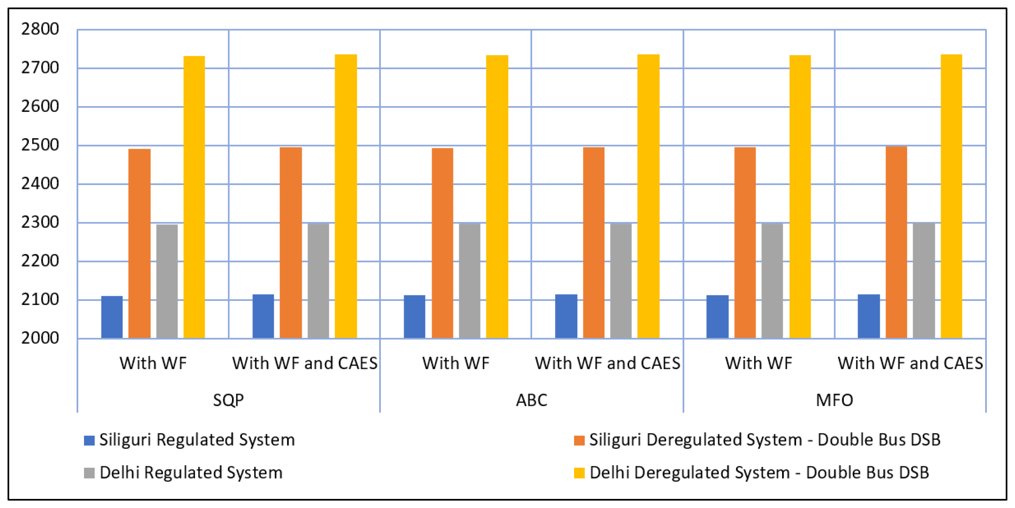
| Average Hourly Profit ($/h) | |||||
|---|---|---|---|---|---|
| Optimization Techniques | Conditions | Siliguri | Delhi | ||
| Regulated System | Deregulated System—Double Bus DSB | Regulated System | Deregulated System—Double Bus DSB | ||
| SQP | With WF | 2111.360 | 2492.157 | 2295.753 | 2732.083 |
| With WF and CAES | 2113.621 | 2495.248 | 2297.547 | 2735.348 | |
| ABC | With WF | 2112.367 | 2493.621 | 2296.547 | 2733.217 |
| With WF and CAES | 2114.626 | 2496.358 | 2298.315 | 2736.629 | |
| MFO | With WF | 2113.455 | 2494.812 | 2297.346 | 2734.328 |
| With WF and CAES | 2115.367 | 2497.924 | 2299.532 | 2736.614 | |
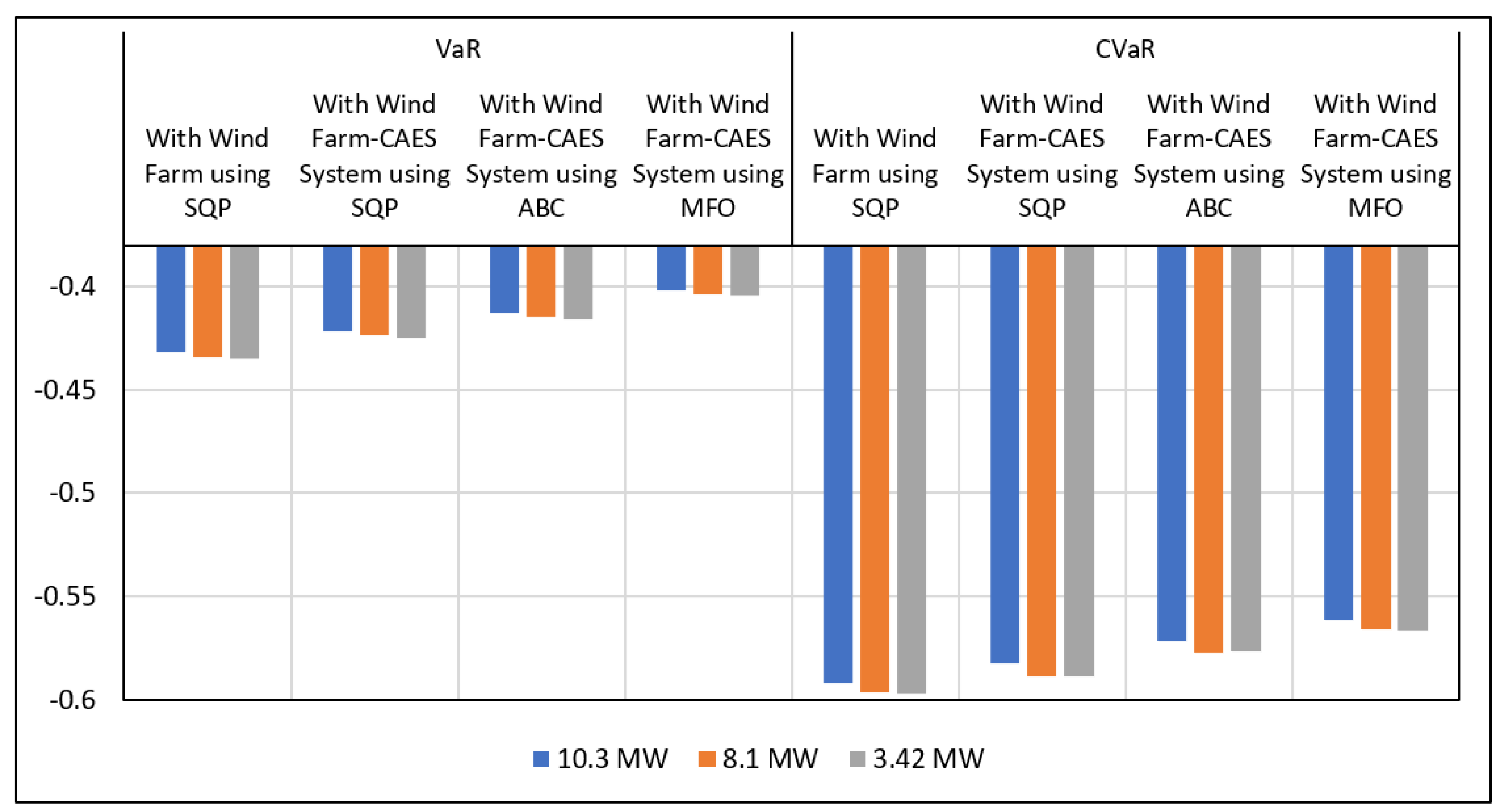
| Sl. No. | Wind Power | VaR | CVaR | ||||||
|---|---|---|---|---|---|---|---|---|---|
| With Wind Farm Using SQP | With Wind Farm-CAES System Using SQP | With Wind Farm-CAES System Using ABC | With Wind Farm-CAES System Using MFO | With Wind Farm Using SQP | With Wind Farm-CAES System Using SQP | With Wind Farm-CAES System Using ABC | With Wind Farm-CAES System Using MFO | ||
| 1 | 10.3 MW | −0.4316 | −0.4214 | −0.4124 | −0.4018 | −0.5918 | −0.5825 | −0.5715 | −0.5615 |
| 2 | 8.1 MW | −0.4345 | −0.4233 | −0.4147 | −0.4037 | −0.5962 | −0.5885 | −0.5773 | −0.5656 |
| 3 | 3.42 MW | −0.4351 | −0.4246 | −0.4158 | −0.4041 | −0.5971 | −0.589 | −0.5764 | −0.5667 |
Publisher’s Note: MDPI stays neutral with regard to jurisdictional claims in published maps and institutional affiliations. |
© 2022 by the authors. Licensee MDPI, Basel, Switzerland. This article is an open access article distributed under the terms and conditions of the Creative Commons Attribution (CC BY) license (https://creativecommons.org/licenses/by/4.0/).
Share and Cite
Chakraborty, M.R.; Dawn, S.; Saha, P.K.; Basu, J.B.; Ustun, T.S. System Profit Improvement of a Thermal–Wind–CAES Hybrid System Considering Imbalance Cost in the Electricity Market. Energies 2022, 15, 9457. https://doi.org/10.3390/en15249457
Chakraborty MR, Dawn S, Saha PK, Basu JB, Ustun TS. System Profit Improvement of a Thermal–Wind–CAES Hybrid System Considering Imbalance Cost in the Electricity Market. Energies. 2022; 15(24):9457. https://doi.org/10.3390/en15249457
Chicago/Turabian StyleChakraborty, Mitul Ranjan, Subhojit Dawn, Pradip Kumar Saha, Jayanta Bhusan Basu, and Taha Selim Ustun. 2022. "System Profit Improvement of a Thermal–Wind–CAES Hybrid System Considering Imbalance Cost in the Electricity Market" Energies 15, no. 24: 9457. https://doi.org/10.3390/en15249457