Study on the Viscosity Optimization of Polymer Solutions in a Heavy Oil Reservoir Based on Process Simulation

Abstract

Polymer flooding has been proved by many scholars for use in heavy oil reservoirs. However, due to mobility control effects and injectivity, selecting the appropriate solution viscosity is essential. It is difficult to form a deep understanding of the effect and mechanism of polymer flooding using conventional experimental methods with oil recovery as the reference standard, so it is necessary to conduct further study with the aid of simulation methods. In this study, a one-dimensional displacement mathematical model based on the Buckley–Leverett theory was established, and in the range of water–oil viscosity ratio from 0.1 to 0.6, the variation of water saturation along the flow caused by polymer solution was studied. The research results showed that under the action of a polymer solution, compared with water flooding, there was a decreasing region of water saturation along the flow due to oil phase accumulation. The larger the water–oil viscosity ratio, the larger the area of water saturation decline and the greater the degree of water saturation decline, resulting in a better the displacement effect. However, under the condition of oil–phase viscosity of 70 mPa·s, when the water–oil viscosity ratio reached 0.4, the range and degree of water saturation decline along the way no longer changed, all the crude oil that could be swept had been displaced, and the outlet end was close to producing only water, not oil; therefore, further increasing the water–oil viscosity ratio could not increase the oil recovery. At the same time, the increase in pressure had not changed, that is, the increase in pressure had not resulted in the same increase in oil recovery. When the viscosity of oil phase increased to 140 mPa·s, the same rule was displayed, the appropriate water–oil viscosity ratio was also 0.4. The paper analyzed the action mechanism of polymer solution through process description, and the results provided a clear selection method for selecting reasonable polymer solution concentration, as well as a reference for polymer solution range under different crude oil viscosity conditions.

1. Introduction

The world is rich in heavy oil resources, and with the development of thin oil reservoirs gradually decline, heavy oil development is becoming increasingly important. In heavy oil development, thermal recovery reduces the oil phase viscosity by heating, which increases the flow capacity of the oil phase and improves the heavy oil recovery [1]. However, for some deep and thin layer heavy oil reservoirs, the development effect is poor due to heat loss [2,3]. Polymer flooding, however, does not have such a problem. By increasing the water-phase viscosity and decreasing the water-oil mobility ratio, polymer flooding can expand the sweep volume and improve oil recovery [4,5]. Polymer flooding has become an important means to develop heavy oil reservoirs [6,7,8,9]. However, for heavy oil reservoirs with high oil phase viscosity, the effect of polymer flooding mobility control is not significant compared with thin oil reservoirs. The effect of polymer flooding with low viscosity is poor, while the injectivity problem may exist with high viscosity [10], so it is necessary to select a reasonable solution viscosity for polymer flooding in heavy oil reservoirs.

In fact, due to the advantages of polymer flooding in enhancing oil recovery, many scholars have conducted relevant research on selecting the polymer flooding solution viscosity [11,12,13]. Based on the field practice of using 30 mPa·s polymer solutions to displace crude oil with a viscosity of 1000 mPa·s in Canadian oilfields [14], and 150 mPa·s polymer solutions to displace crude oil with a viscosity of 10 mPa·s in Daqing oilfields in China [15], Seright [16] proposed the research question asking how much the polymer solution viscosity should be when polymer flooding is carried out, and conducted the relevant analysis from the perspectives of water-oil mobility ratio, injection pressure and economic benefits. Furthermore, in 2018, Seright et al. [17] proposed through research that, when displacing crude oil with a viscosity of 1610 mPa·s, using a polymer solution with a viscosity of 25 mPa·s could improve oil recovery. However, when the polymer solution viscosity was increased further, the effect was not obvious. Therefore, they investigated the cause of this phenomenon and indicated that the reason for this phenomenon was the influence of the oil-water relative permeability value; that is, the water phase relative permeability value was low. Levitt et al. [18] also found that when the crude oil viscosity was 2000~5000 mPa·s and a 2 PV polymer solution was injected, when the solution viscosity increased from 3 mPa·s to 60 mPa·s, there would be no significant change in oil recovery.

Many experiments have been carried out to obtain the appropriate polymer solution viscosity that matches with the viscosity of crude oil. Wang et al. [19,20] conducted 28 groups of sand pack model oil displacement experiments. Within a crude oil viscosity range of 430 mPa·s to 5500 mPa·s, the incremental oil recovery obtained from polymer solution displacement experiments under different viscosity conditions showed an S-shaped change; that is, there were minimum and optimal values to improve the displacement effect. The minimum value means that there is no oil increase effect below this value, while the optimal value means that the recovery factor will not change greatly when this value is exceeded. On this basis, Guo et al. [21] used the mobility ratio at the end of water flooding as the normalization factor, and plotted the recovery factor and normalization factor obtained under different crude oil viscosity and polymer solution viscosity conditions in the same coordinate axis, so as to obtain the relationship between the polymer flooding recovery factor and the normalization factor, and to evaluate the potential of using polymer flooding for heavy oil.

In existing studies on the selection of polymer solution under different crude oil viscosity conditions, most used oil recovery as a reference index to judge whether the selection of polymer solution was appropriate [22]. Olayiwola and Dejam [23] used laboratory experiments to study the oil recovery performance of alternate injection of silica NPS, LSW and sodium dodecyl sulfate (SDS) surfactant to judge reasonable injection methods. Zhu et al. [24] studied the influence of polymer solution viscosity and residual resistance factor on injection pressure and oil recovery through displacement experiment. Although the oil recovery was an important parameter, it only reflected the polymer flooding results. Combined with the selection of polymer solution viscosity at the injection end, the existing studies [13,25,26] mainly focused on the parameter description of the injection and production ends, but did not analyze the parameter changes during the displacement process. The study of the parameter changes in the displacement process was conducive to an in-depth understanding of the process of polymer flooding under different crude oil viscosity conditions, and an analysis of its displacement mechanism.

However, it is difficult to quantitatively analyze the parameter changes in the process of displacement through conventional physical experiments, so it is necessary to study it by means of simulation. In this paper, with the help of simulation software (COMSOL) [27,28], a mathematical model was established using a custom partial differential equation (PDE) to study the variation in water saturation along the flow caused by polymer flooding in a one-dimensional displacement process. The mechanism of selecting the appropriate polymer solution viscosity under different crude oil viscosity conditions was analyzed by combining the oil recovery and water cut, to provide a reference for the selection of polymer solution under different crude oil viscosity conditions. Through this study, we can have a clear understanding of the oil displacement process of polymer solution, so as to select reasonable polymer solution concentration for different conditions and improve the application effect of polymer solution. The research roadmap is shown in Figure 1.

2. Experiments and Methodology

2.1. Measurement of Relative Permeability Curve

2.1.1. Materials

Experimental Core

An artificial homogeneous core (4.5 cm × 4.5 cm × 30 cm) is made by pressing quartz sand of the same mesh, which is used for the determination of relative permeability. The permeability of the core is approximately 2500 mD and the porosity is about 30%.

Brine

The composition of the brine used in the experiments is listed in

Table 1. Brine composition.

Ion Types	Na+, K+	Ca2+	Mg2+	CO32−	HCO3−	SO42−	Cl−	TDS
Concentration (mg/L)	3091.96	276.16	158.68	14.21	311.48	85.29	5436.34	9374.12

, the brine is used for water flooding experiment and polymer solution preparation.

Oil

The oil used in the experiment is crude oil taken from the oil field. After dehydration, it is diluted with diesel oil to make viscosity being 70 mPa·s at 65 °C.

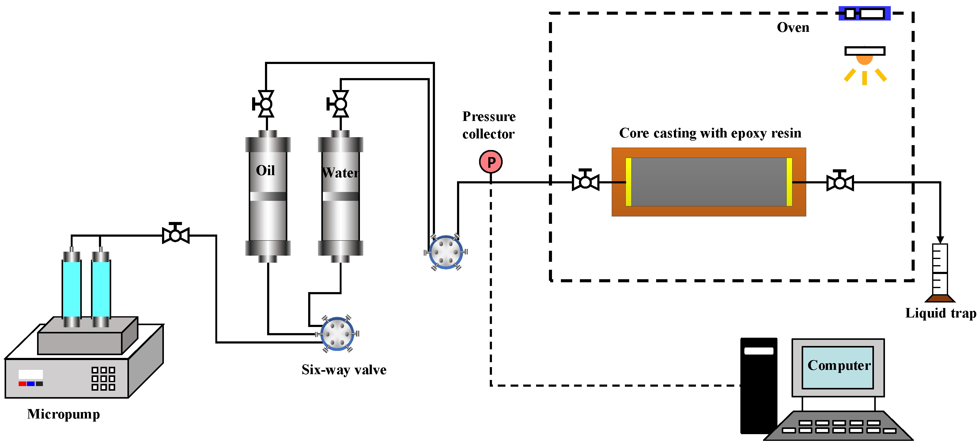
2.1.2. Experimental Procedures

(1)

Drain the saturated core with oil: the gradient flow rate method was used to flood the core with oil, the flow rates were 0.1 mL/min, 0.2 mL/min, 0.5 mL/min and 1.0 mL/min, successively. At each flow rate, the core was saturated with oil until the pressure was stable and no water was produced, then the water and oil production and displacement pressure data were collected [23].

(2)

Water flooding: Water displacement was carried out at a flow rate of 1.0 mL/min until the pressure was stable and no oil was produced. Water and oil production and displacement pressure data were collected. The experimental flowchart is presented in Figure 2.

(3)

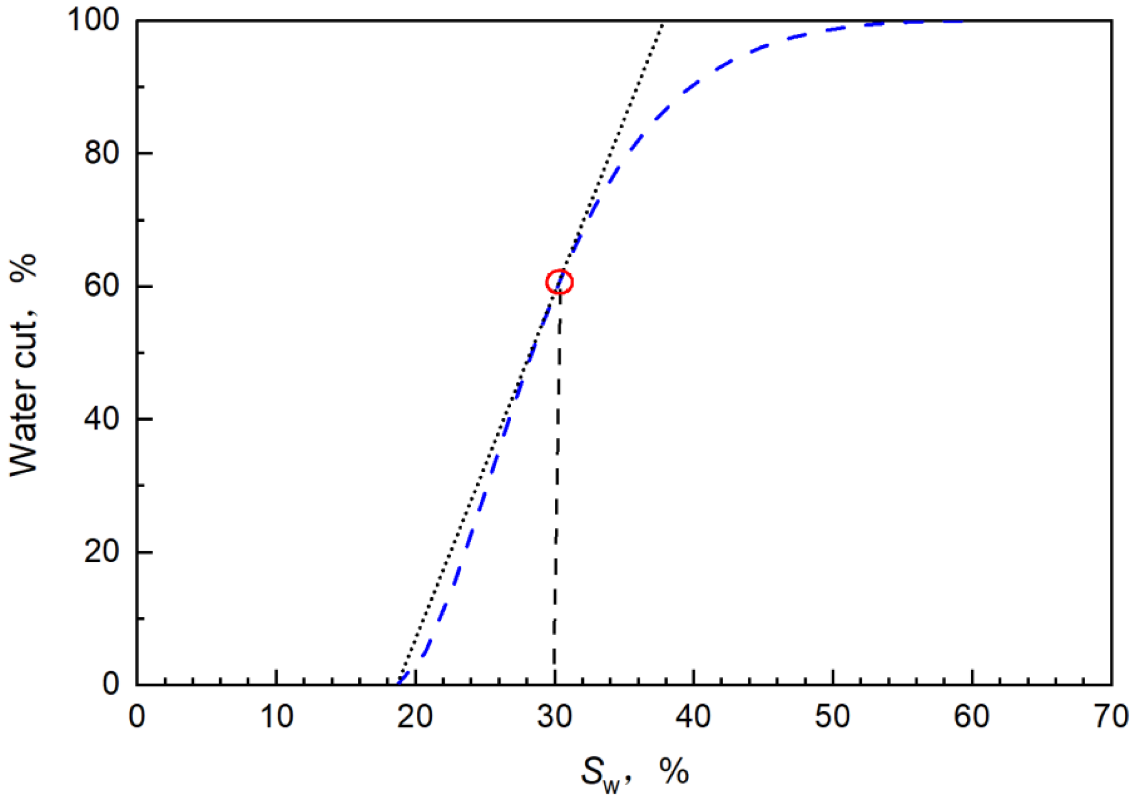
Data processing: The JBN method was used to process the displacement data, then the relative permeability curve was standardized according to the Corey model.

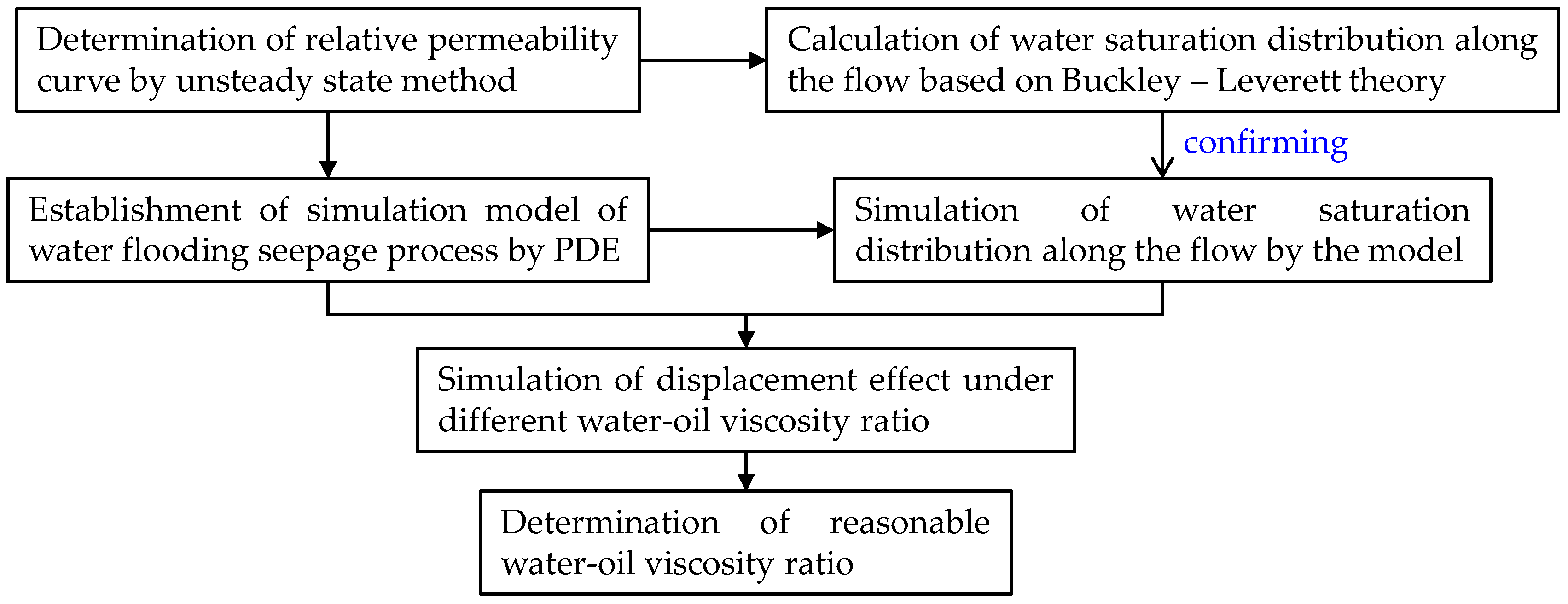
2.2. Numerical Simulation

2.2.1. Model Building

To simulate the seepage process of water flooding, a homogeneous model was established with a size of 30 cm × 4.5 cm, a permeability of 2500 mD and a porosity of 30%, as shown in Figure 3.

The displacement was carried out by means of a constant flow rate at the inlet end and constant pressure at the outlet end. The flow rate was converted to 8.23 × 10⁻⁶ m/s through 1 mL/min in the physical experiment, and the outlet pressure was set to 0 mPa. The injection time was set as 180 min, which was converted into dimensionless time, namely the multiple of pore volume, as shown in Equation (1), then 180 min was approximately 1 PV:

$${\mathrm{t}}_{\mathrm{D}}=\frac{\mathrm{v}\cdot \mathrm{t}}{\mathsf{\varphi }\cdot \mathrm{L}}$$

(1)

where v represents the flow rate (m/s), t is the injection time (s), ϕ denotes the porosity and L stands for the length of the model (m).

The equations of motion and continuity of the two phases of oil and water were rewritten into partial differential equations (PDE), and the mathematical model was established with the PDE module in COMSOL.

According to the continuity equation and the motion equation of the oil-water two-phase flow, Equations (2) and (3) can be obtained:

$$\mathsf{\varphi }\frac{\mathsf{\partial }{\mathrm{S}}_{\mathrm{w}}}{\partial \mathrm{t}}+\frac{\partial {\mathrm{v}}_{\mathrm{w}}}{\partial \mathrm{x}}=\mathsf{\varphi }\frac{\partial {\mathrm{S}}_{\mathrm{w}}}{\partial \mathrm{t}}-\frac{\partial \left(\frac{\mathrm{K}\cdot {\mathrm{K}}_{\mathrm{rw}}}{{\mathsf{\mu }}_{\mathrm{w}}}\cdot \frac{\partial \mathrm{p}}{\partial \mathrm{x}}\right)}{\partial \mathrm{x}}=0$$

(2)

$$\mathsf{\varphi }\frac{\partial {\mathrm{S}}_{\mathrm{o}}}{\partial \mathrm{t}}+\frac{\partial {\mathrm{v}}_{\mathrm{o}}}{\partial \mathrm{x}}=-\mathsf{\varphi }\frac{\partial {\mathrm{S}}_{\mathrm{w}}}{\partial \mathrm{t}}-\frac{\partial \left(\frac{\mathrm{K}\cdot {\mathrm{K}}_{\mathrm{ro}}}{{\mathsf{\mu }}_{\mathrm{o}}}\cdot \frac{\partial \mathrm{p}}{\partial \mathrm{x}}\right)}{\partial \mathrm{x}}=0$$

(3)

where S_w represents the water saturation; S_o stands for the oil saturation; v_o and v_w denote the seepage velocity of the oil phase and water phase, respectively; K is the permeability; K_ro refers to the oil phase relative permeability; K_rw represents the water phase relative permeability, μ_o and μ_w are the viscosity of oil phase and water phase, respectively; and p indicates the pressure.

When a polymer solution is used, the concentration convection diffusion equation is coupled, as shown in Equation (4):

$$\mathsf{\varphi }\frac{\partial {\mathrm{C}}_{\mathrm{p}}}{\partial \mathrm{t}}=\mathrm{D}\frac{{\partial }^2{\mathrm{C}}_{\mathrm{p}}}{\partial {\mathrm{x}}^2}-\mathrm{v}\frac{\partial {\mathrm{C}}_{\mathrm{p}}}{\partial \mathrm{t}}$$

(4)

where C_p represents the polymer solution concentration, D denotes the diffusion coefficient.

For conventional polymer solutions, the solution performance is a function of concentration. For example, the relationship between the viscosity and concentration of the solution is shown in Equation (5).

$${\mathsf{\mu }}_{\mathrm{p}}=\mathrm{k}\cdot {\mathrm{C}}_{\mathrm{p}}+0.001$$

(5)

where k is the slope of viscosity-concentration relationship curve.

Therefore, during the displacement process, the viscosity will change with the change of solution concentration.

The form of the coefficient form partial differential equation is shown in Equation (6).

$${\mathrm{e}}_{\mathrm{a}}\frac{{\partial }^2\mathrm{u}}{{\partial }^2\mathrm{t}}+{\mathrm{d}}_{\mathrm{a}}\frac{\partial \mathrm{u}}{\partial \mathrm{t}}-\nabla \cdot (\mathrm{c}\nabla \mathrm{u}+\mathrm{a}\mathrm{u}-\mathsf{\gamma })+\mathsf{\beta }\cdot \nabla \mathrm{u}+\mathrm{a}\mathrm{u}=\mathrm{f}$$

(6)

where u represents the dependent variable; ${\mathrm{e}}_{\mathrm{a}}\frac{{\partial }^2\mathrm{u}}{{\partial }^2\mathrm{t}}$ denotes a quality item; ${\mathrm{d}}_{\mathrm{a}}\frac{\partial \mathrm{u}}{\partial \mathrm{t}}$ indicates a storage item; $\mathrm{c}\nabla \mathrm{u}+\mathrm{a}\mathrm{u}-\mathsf{\gamma }$ refers to the conservation flux, where each item in turn represents the diffusion term, convection term and source term; $\mathsf{\beta }\cdot \nabla \mathrm{u}$ represents the convection term; $\mathrm{a}\mathrm{u}$ stands for absorbing term; and f is the source item.

Therefore, the equations of motion and continuity of the two phases of oil and water and concentration equations are rewritten into partial differential equations, and the coefficients are shown in Equation (7):

$$\mathrm{u}=\left[\begin{array}{c}{\mathrm{S}}_{\mathrm{w}}\\ \mathrm{p}\end{array}\right]\frac{\partial \mathrm{u}}{\partial \mathrm{t}}=\left[\begin{array}{c}\frac{\partial {\mathrm{S}}_{\mathrm{w}}}{\partial \mathrm{t}}\\ \frac{\partial \mathrm{p}}{\partial \mathrm{t}}\end{array}\right]\mathrm{d}\mathrm{a}=\left[\begin{array}{cc}\mathsf{\varphi }& 0\\ 0& 0\end{array}\right]\mathrm{c}=\left[\begin{array}{cc}0& \frac{\mathrm{K}\cdot {\mathrm{K}}_{\mathrm{rw}}}{{\mathsf{\mu }}_{\mathrm{p}}({\mathrm{C}}_{\mathrm{p}})\cdot {\mathrm{R}}_{\mathrm{k}}}\\ 0& \frac{\mathrm{K}\cdot {\mathrm{K}}_{\mathrm{rw}}}{{\mathsf{\mu }}_{\mathrm{p}}({\mathrm{C}}_{\mathrm{p}})\cdot {\mathrm{R}}_{\mathrm{k}}}+\frac{\mathrm{K}\cdot {\mathrm{K}}_{\mathrm{ro}}}{{\mathsf{\mu }}_{\mathrm{o}}}\end{array}\right]$$

(7)

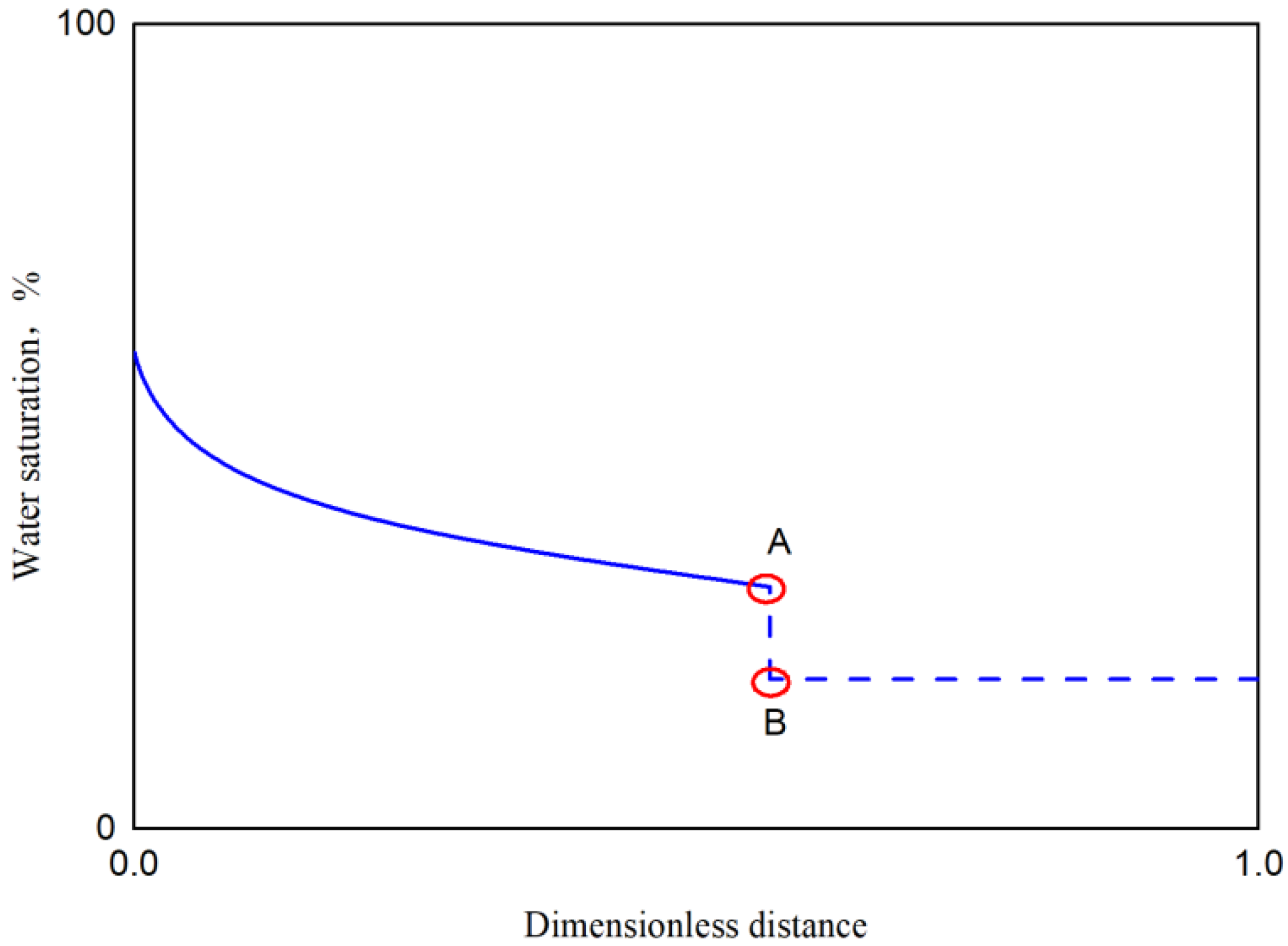
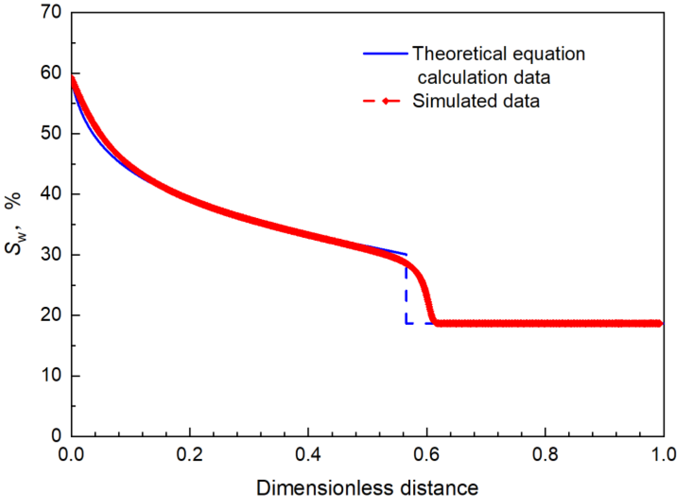
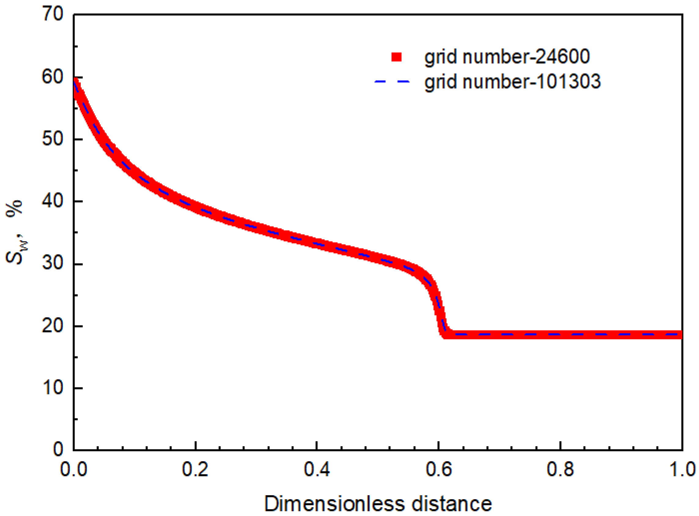
2.2.2. Model Validation

Under the condition of neglecting capillary pressure and gravity, the water saturation along the flow can be obtained through an oil-water seepage equation, according to the Buckley-Leverett theory and the calculation of the relative permeability curve, as shown in Equation (8):

$$\frac{\mathrm{d}\mathrm{x}}{\mathrm{d}\mathrm{t}}=-\frac{\frac{\partial {\mathrm{S}}_{\mathrm{w}}}{\partial \mathrm{t}}}{\frac{\partial {\mathrm{S}}_{\mathrm{w}}}{\partial \mathrm{x}}}=\frac{\mathrm{v}}{\mathsf{\varphi }}{{\mathrm{f}}_{\mathrm{w}}}^{\prime }\left({\mathrm{S}}_{\mathrm{w}}\right)$$

(8)

Through the relative permeability curve, the relationship curve between water saturation and water cut can be calculated to obtain the derivative of water cut, and then the displacement distance at a certain moment can be obtained, the specific calculation process will be described in detail in the subsequent experimental part. So that the corresponding relationship between water saturation and displacement distance can be obtained, that is, the distribution of water saturation along the flow. The schematic diagram is shown in Figure 4, where the water saturation along the flow gradually decreases. According to the Buckley-Leverett theory, the displacement front always moves forward at a fixed water saturation and a fixed speed; that is, in the process of oil displacement, the saturation of the displacement agent changes from the water saturation of the displacement front to irreducible water saturation prior to there being no water at the outlet end of the model, as shown in point A and point B in Figure 4.

The accuracy of the model can be verified by comparing it with the water saturation along the flow obtained using the simulation calculation.

2.2.3. Simulation of the Effect of Viscosity on Displacement Process and Effect

To observe the overall process of water flooding, displacement agent flooding and subsequent water flooding with a total injection volume of 1.00 PV (Pore Volume), a displacement agent solution with a certain viscosity was injected after 0.18 PV of water flooding. After the injection volume of the displacement agent solution reached 0.10 PV, we transferred to subsequent water flooding. By setting different viscosity values for the displacement agent solution, the influence of viscosity on the displacement process, including water saturation along the flow and recovery, was simulated and studied. The viscosity ratios of the displacement fluid and oil were set as 0.1, 0.2, 0.3, 0.4 and 0.5, respectively.

3. Results and Discussions

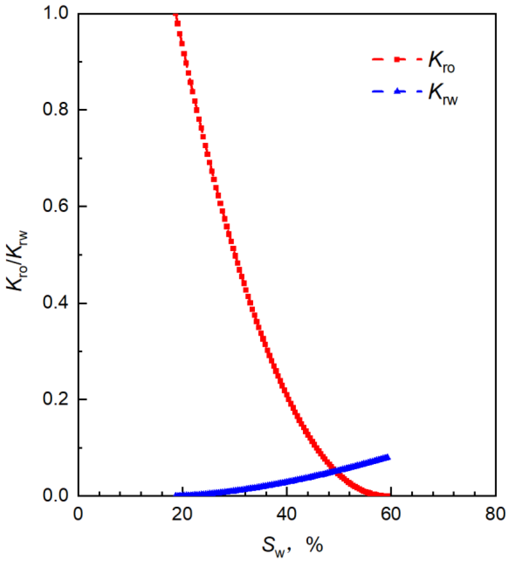
3.1. Oil-Water Relative Permeability Curve

Through the relative permeability curve, the displacement effect can be calculated theoretically, and the relative permeability curve is also one of the most important parameters for establishing the seepage model [29]. Measured using the unsteady state method [30], the oil-water relative permeability curve treated using the JBN method [31] and the Corey model is shown in Figure 5, and the relevant parameters are shown in

Table 2. Relevant parameters of the oil-water relative permeability curve.

Swi	Sor	Kro (Swi)	Krw (Sor)	no	nw
0.19	0.41	1.00	0.08	2.10	1.60

.

Where S_wi represents the irreducible water saturation, S_or stands for the residual oil saturation, K_ro (S_wi) is the oil phase relative permeability at the irreducible water saturation, K_rw (S_or) denotes the water phase relative permeability at the residual oil saturation, no represents the index of the oil phase and nw refers to the index of the water phase.

In the process of water flooding, the relative permeability of the oil phase decreases and the relative permeability of the water phase increases with the increase in water saturation. Through the relative permeability value, the change in the water cut with water saturation can be calculated, as shown in Equation (9):

$${\mathrm{f}}_{\mathrm{w}}=\frac{1}{1+\frac{{\mathrm{K}}_{\mathrm{ro}}}{{\mathrm{K}}_{\mathrm{rw}}}\cdot \frac{{\mathsf{\mu }}_{\mathrm{w}}}{{\mathsf{\mu }}_{\mathrm{o}}}}$$

(9)

The water saturation of the displacement front can then be calculated according to the water cut, as shown in Equation (10) and Figure 6:

$${\mathrm{S}}_{\mathrm{wf}}=\frac{{\mathrm{f}}_{\mathrm{w}}\left({\mathrm{S}}_{\mathrm{wf}}\right)}{{{\mathrm{f}}_{\mathrm{w}}}^{\prime }\left({\mathrm{S}}_{\mathrm{wf}}\right)}+{\mathrm{S}}_{\mathrm{wi}}$$

(10)

When the tangent of the curve of the water cut changing with water saturation is made from the irreducible water saturation (S_wi) point, the water saturation corresponding to the tangent point is the water saturation of the displacement front (S_wf), which is 30%. In Equation (10), f_w (S_wf) represents the water cut corresponding to the water saturation of the displacement front and ${{\mathrm{f}}_{\mathrm{w}}}^{\prime }\left({\mathrm{S}}_{\mathrm{wf}}\right)$ denotes the slope of the above tangent, which is 5.16.

When the displacement time was 0.11 PV (20 min), the position of the displacement front (the water saturation is 30%) at this time could be calculated according to Equation (8), as shown in Equation (11).

$${\mathrm{x}}_{\mathrm{D}}=\frac{\mathrm{vt}}{\varnothing }{{\mathrm{f}}_{\mathrm{w}}}^{\prime }\left({\mathrm{S}}_{\mathrm{wf}}\right)/\mathrm{L}=\frac{8.26\times {10}^{-6}\times 20\times 60}{0.3}\times 5.16/0.3=0.57$$

(11)

That is to say, the displacement front was at the dimensionless distance of 0.57, and other water saturation positions could also be obtained, as shown in Figure 7.

3.2. Model Validation

The established model was used for the displacement simulation. When the displacement time reached approximately 0.11 PV, the simulated water saturation along the flow was compared with the water saturation obtained by theoretical calculation to verify the accuracy of the model, as shown in Figure 8.

As can be seen from Figure 8, the simulated water saturation distribution along the flow basically coincides with the theoretical calculation, except that there is a difference when the water saturation is approximately 30%, this water saturation corresponds to the displacement front. From the simulation point of view, in the calculation process, because the equation is solved numerically, and the water saturation near the front edge will be automatically interpolated for calculation, there will be no sudden change in data, so there is a difference between the simulation data and the theoretical calculation data at the front of the displacement. However, the error is only about 5%, which does not affect the research results. Therefore, the model can effectively reflect the change in water saturation along the flow, and the results are accurate.

To verify the reliability of the model, we used the results of different densified grids for comparison, as shown in Figure 9. The results of different densified grids were basically consistent, indicating that the calculation results of the model were reliable.

3.3. Study on the Influence of Different Viscosity Conditions on the Seepage Process

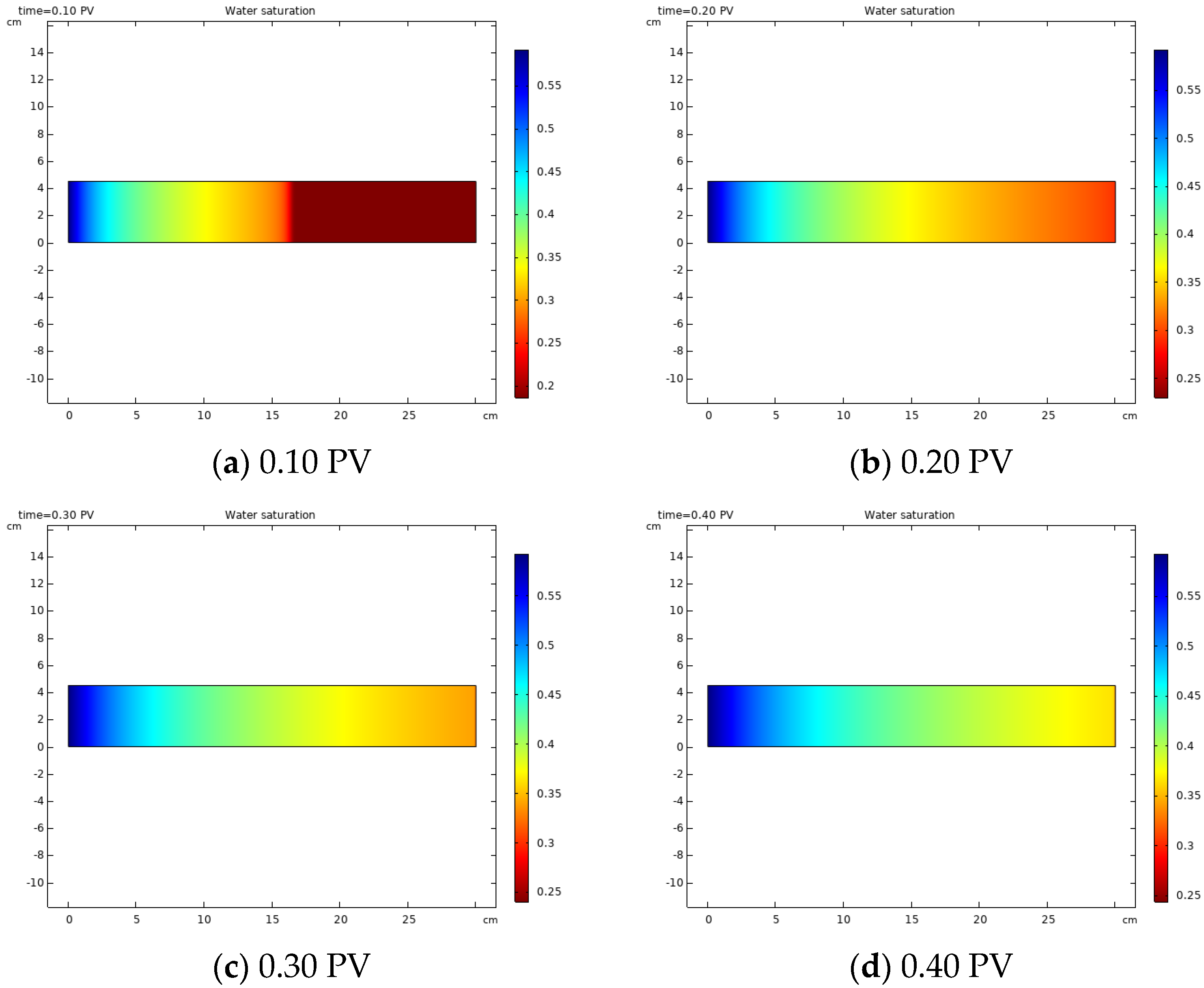
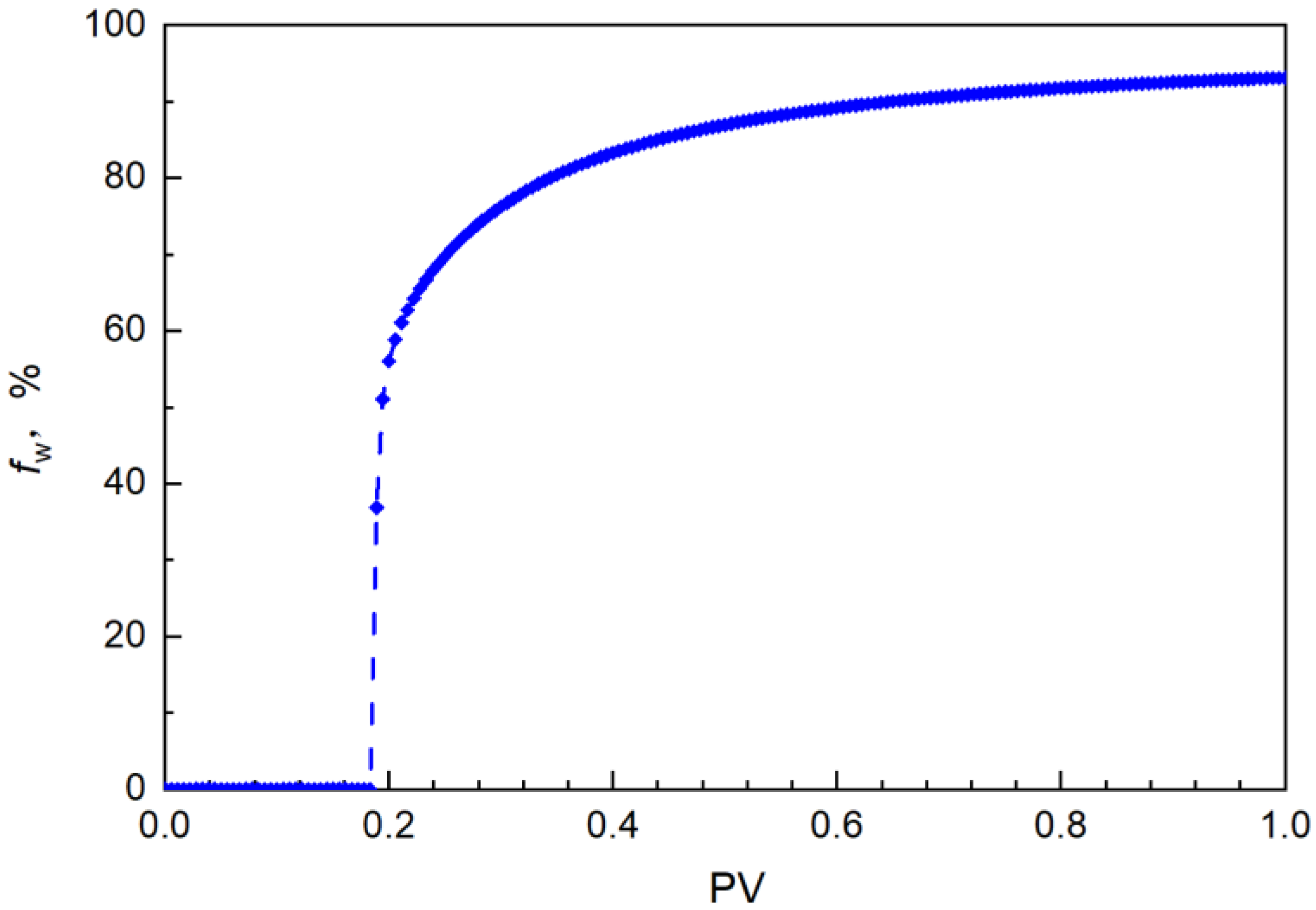
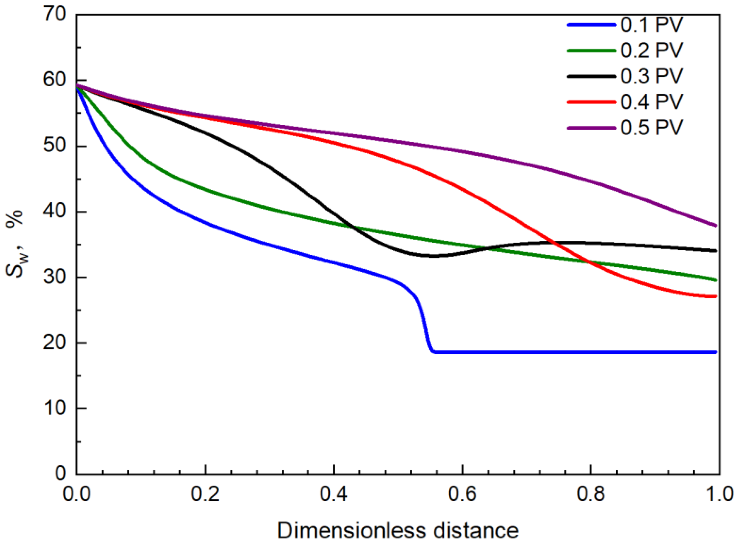
3.3.1. Simulation of the Water Flooding Process

During water flooding, the water saturation changes with the extension of the displacement time, as shown in Figure 10.

In Figure 10, blue represents displacement agent and red represents oil. From the color change in the simulation results, it can be seen that, with displacement, the oil saturation in the model decreased and the water phase saturation increased. In Figure 10a, the section from blue to red represented that the water phase had swept to this position, while the unchanged red area represented that the water phase had not swept, that is, the water displacement front was located in the middle of the model and the dimensionless distance calculated in Equation (11) was 0.57. From Figure 10b to Figure 10d, the red color changed, indicating that the water phase had reached the outlet end, and different water saturation made the color change different.

As it was under the homogeneous model conditions, the vertical saturation distribution was uniform. With a further extension of the displacement time, the water saturation along the flow showed a slow growth trend. The closer it was to the inlet end, the higher the water saturation, that is, the more oil phase was displaced. The results accorded with the variation law of water flooding.

The distribution of water saturation along the flow under different displacement time is shown in Figure 11.

When the displacement time was 0.10 PV, the position of the water displacement front reached a dimensionless distance of 0.57. When the displacement time was 0.20 PV, the water saturation along the flow was higher than that of the displacement front (30%), indicating that the water phase reached the outlet end, completing the breakthrough. Additionally, it can be seen from Figure 12 that the time for the water phase to reach the outlet end was approximately 0.18 PV, the water cut at the outlet end increased rapidly.

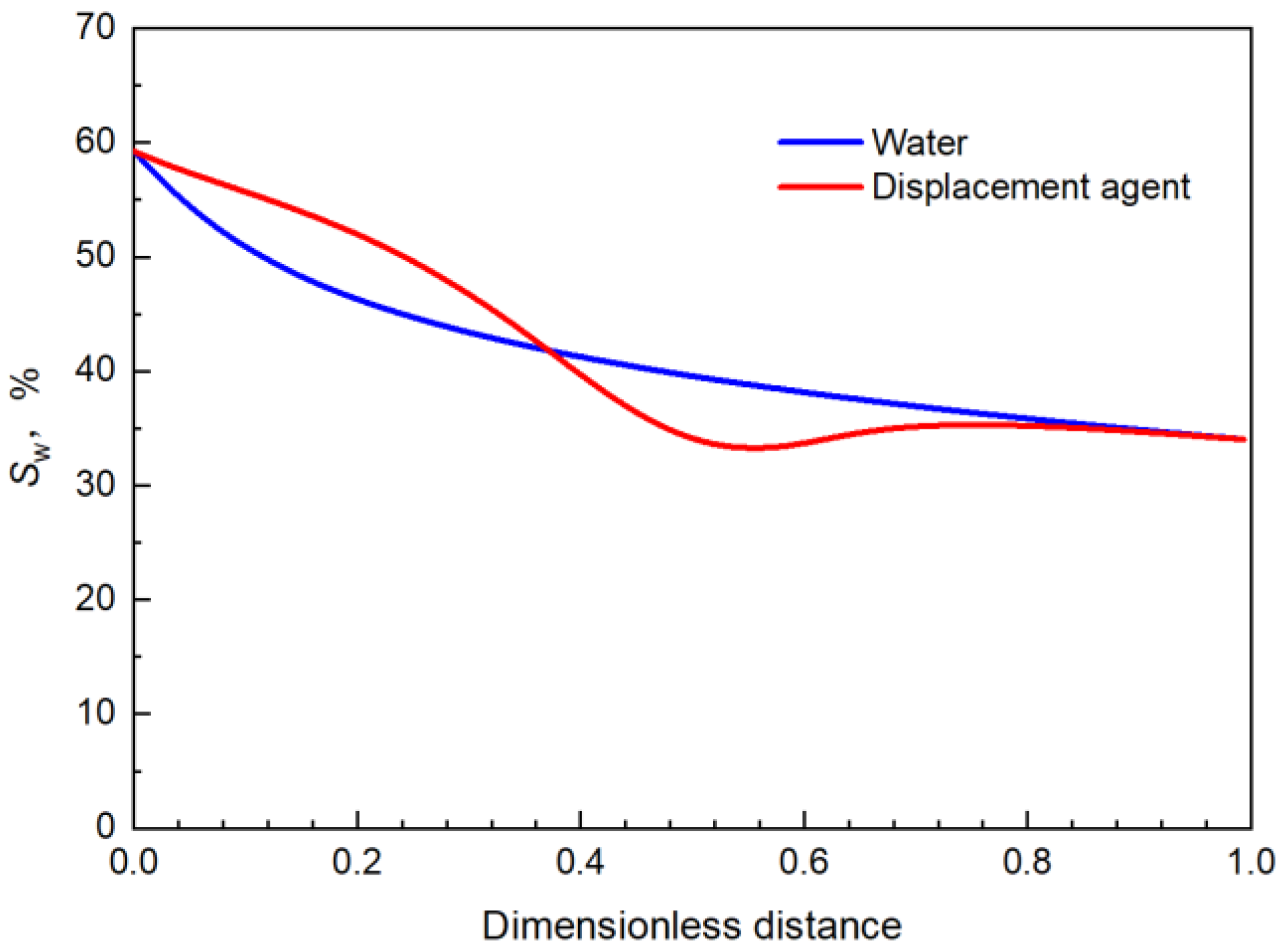
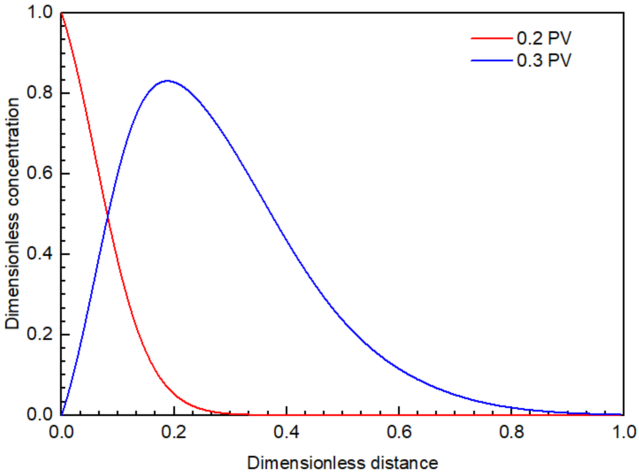
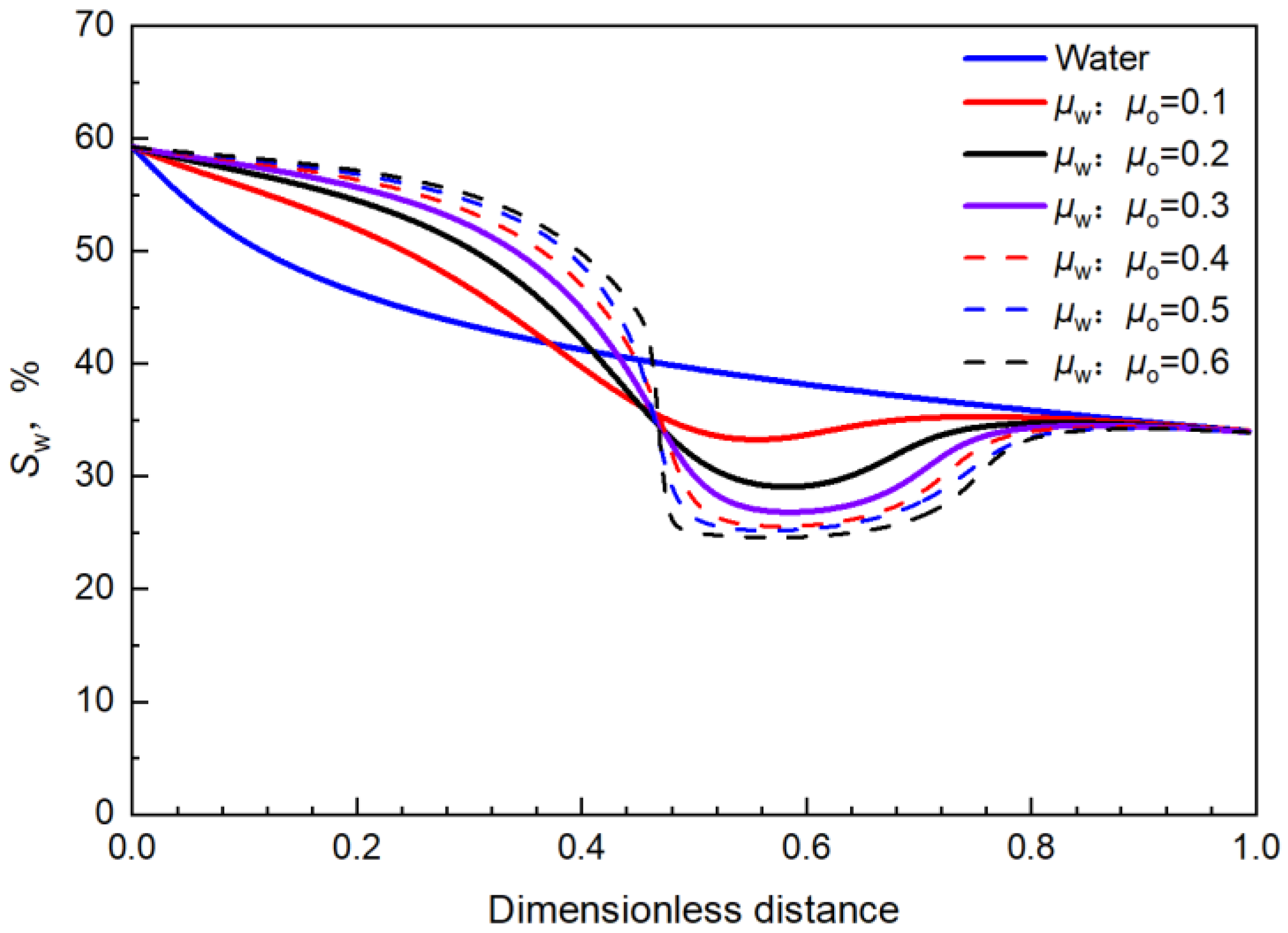
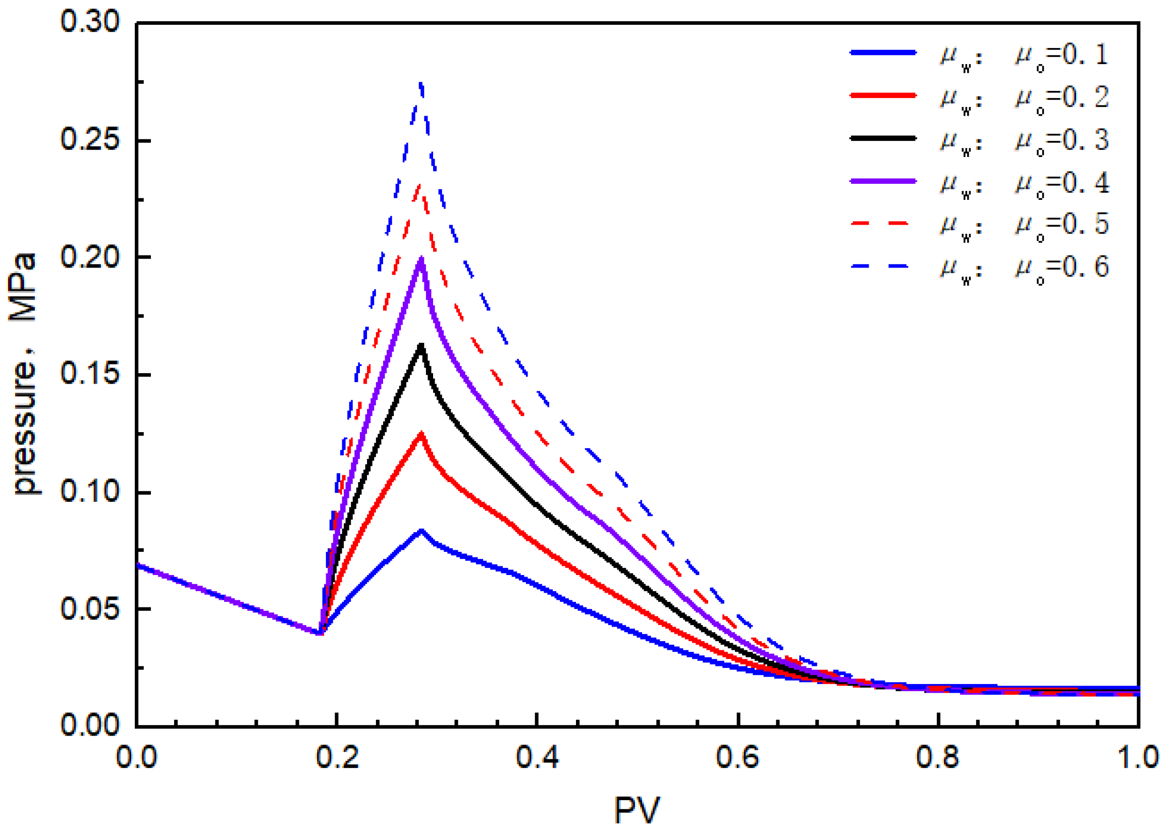
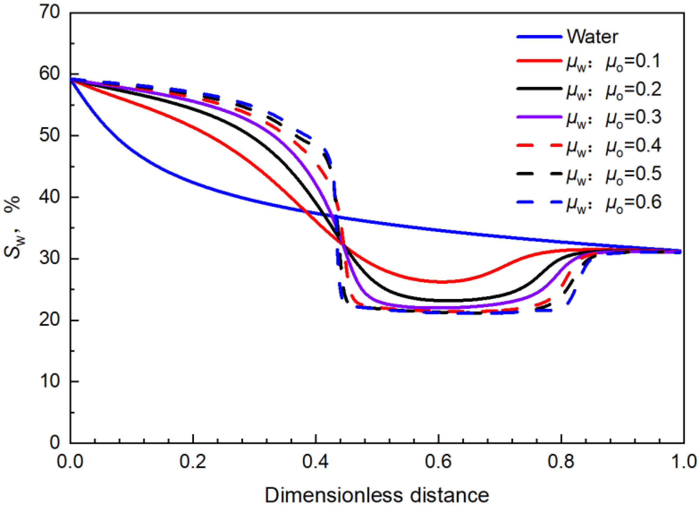
3.3.2. Simulation the Process of Polymer Flooding after Water Flooding

When 0.10 PV of displacement agent was injected after 0.18 PV of water flooding, the change in water saturation along the flow resulted due to the mobility control effect of the displacement agent, which was different from the change law of water flooding. There was an area where the water saturation decreased due to the mobility control effect [24]. Taking the ratio of displacement agent viscosity to crude oil viscosity as 0.1 as an example, the variation in water saturation is shown in Figure 13.

It can be clearly seen from Figure 13b that the water saturation at the dimensionless distance of approximately 0.53 (16 cm) was less than that at the same position in Figure 13a; that is, with the displacement, there was a decrease in water saturation at some positions.

Since it was a displacement agent transferred at 0.18 PV, the distribution of water saturation along the flow at 0.1 PV and 0.18 PV was consistent with water flooding. However, when the displacement time reached 0.3 PV, since the displacement agent had played the role of mobility control, more oil was displaced from the inlet end, so as to reduce the oil phase saturation near the inlet end and increase the water saturation. Therefore, the water saturation change in Figure 14 occurred when the dimensionless distance was less than 0.38.

As the oil phase accumulated and advanced continuously, the water saturation decreased when the dimensionless distance was greater than 0.38 and less than 0.80, as shown in Figure 14. However, when the dimensionless distance was greater than 0.80, the water saturation distribution was the same as that of water flooding, which indicated that the mobility control function of the displacement agent did not affect this part at this time [32].

Further, we analyzed the concentration of polymer solution along the flow when the displacement time reached 0.3 PV, as shown in Figure 15.

It can be seen from Figure 15 that, when polymer solution was injected, the concentration at the inlet end was the highest. Along the displacement direction, the concentration gradually decreased. When the concentration was 0, it indicated that the polymer solution had not reached this position. With the extension of displacement time, when it increased from 0.2 PV to 0.3 PV, the polymer solution concentration at the inlet end became 0 due to the subsequent water flooding, and the highest solution concentration along the flow decreased. When the dimensionless distance was greater than 0.80, the concentration of polymer solution became approximately 0, this also indicated that the mobility control function of the polymer solution did not affect the part.

The variation in water saturation along the flow under different displacement times is shown in Figure 16.

Comparing the water saturation along the flow with different displacement times, when the displacement time increased from 0.2 PV to 0.3 PV, the water saturation at the dimensionless distance 0.44 to 0.64 decreased, it could also be seen from Figure 15 that the polymer solution had reached this section; but when the displacement time increased from 0.3 PV to 0.4 PV, the water saturation at this section increased. Since polymer flooding was switched after water injection of 0.18 PV, when the displacement time increased from 0.2 PV to 0.3 PV, the water saturation decreased due to the mobility control, while the subsequent water flooding was switched at 0.28 PV, so the water saturation increased when the displacement time increased from 0.3 PV to 0.4 PV. Additionally, it could be seen that the low water saturation area was advancing continuously, reflecting the process of the oil phase being pushed forward.

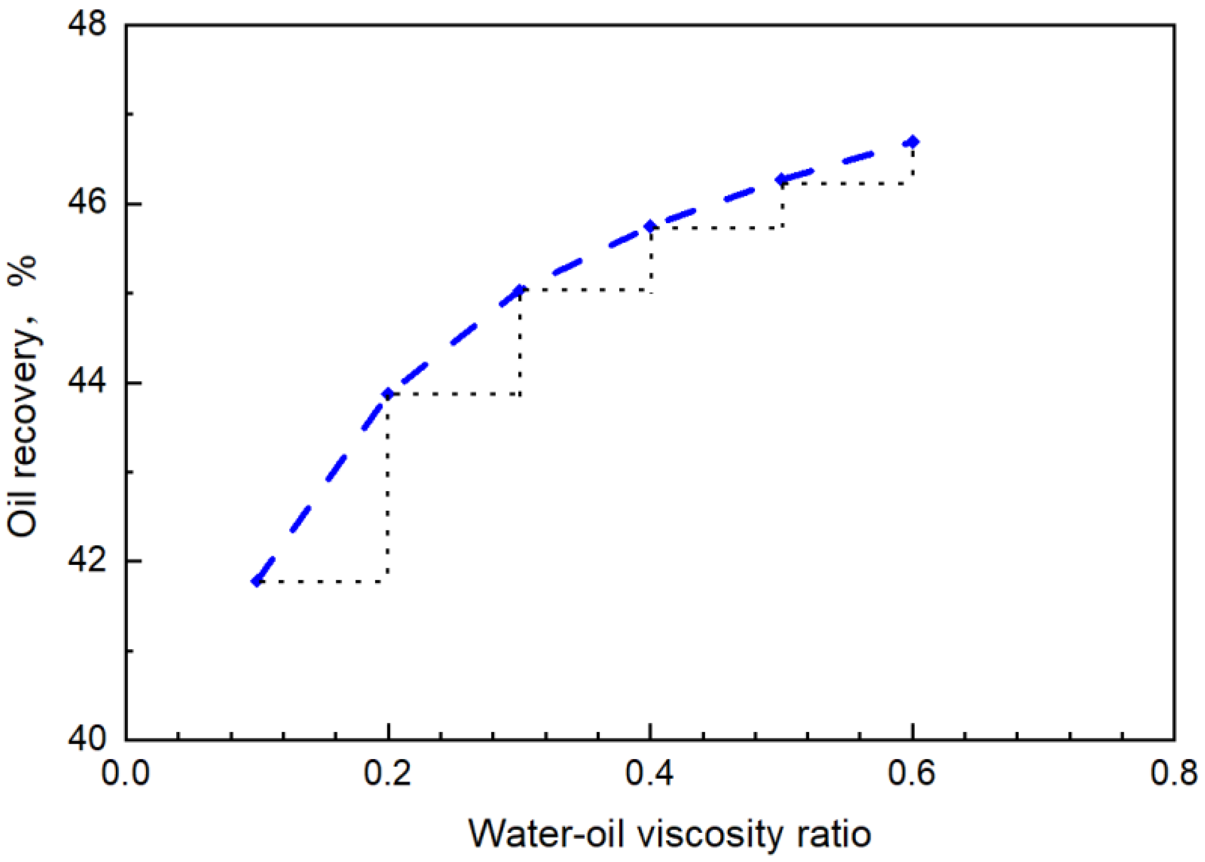
3.3.3. Comparison of Oil Displacement Effect under Different Water-Oil Viscosity Ratio Conditions

We compared the water saturation distribution along the flow under different water-oil viscosity ratio conditions, as shown in Figure 17.

It can be seen from Figure 17 that, in the water saturation decreasing section, with the increase in the water-oil viscosity ratio, the greater the degree of decrease in the water saturation, that is, the stronger the mobility control effect. At the same time, it can also be clearly seen that, when the water-oil viscosity ratio was 0.4~0.6, the degree of decrease in water saturation did not differ greatly; that is, further increasing the water phase viscosity did not produce a great effect.

The change curves of the water cut under different viscosity conditions are shown in Figure 18.

It can also be seen from the changes in the water cut that, with the increase in water phase viscosity, the greater the decrease in the water cut and the better the effect. When the water-oil viscosity ratio exceeded 0.4, the displacement effect would not change greatly.

The oil recovery under different water-oil viscosity ratios is shown in Figure 19.

According to the comparison of oil recovery under different water-oil viscosity ratios, with the increase in the water-oil viscosity ratio, the recovery efficiency showed an increasing trend, but the increasing effect gradually weakened. In combination with the change law of water cut and water saturation along the flow, under such conditions, the appropriate water-oil viscosity ratio in the process of displacement should not exceed 0.4.

Further, we compared the injection pressure under different water-oil viscosity ratios, as shown in Figure 20.

From the perspective of injection pressure, the injection pressure increased due to polymer flooding, and decreased due to subsequent water flooding. The higher the water oil viscosity ratio was, the faster the injection pressure rose and the higher the maximum pressure was. By comparing the injection pressure under different water oil viscosity ratios, it can be seen that the maximum value basically showed a linear growth, while in combination with the change of oil recovery, the increase in injection pressure did not produce the same amplitude of oil recovery growth. In combination with the injection pressure, the optimal water-oil viscosity ratio was not more than 0.4.

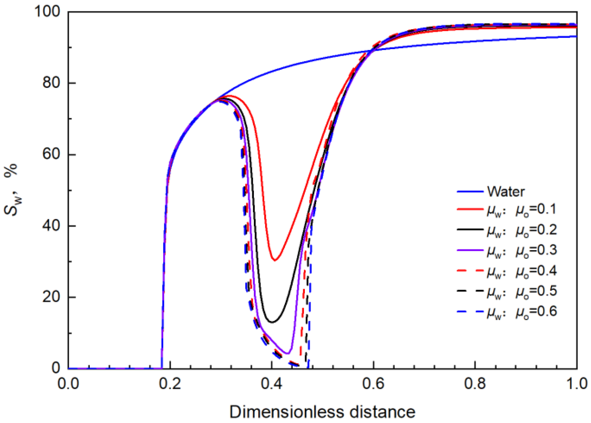
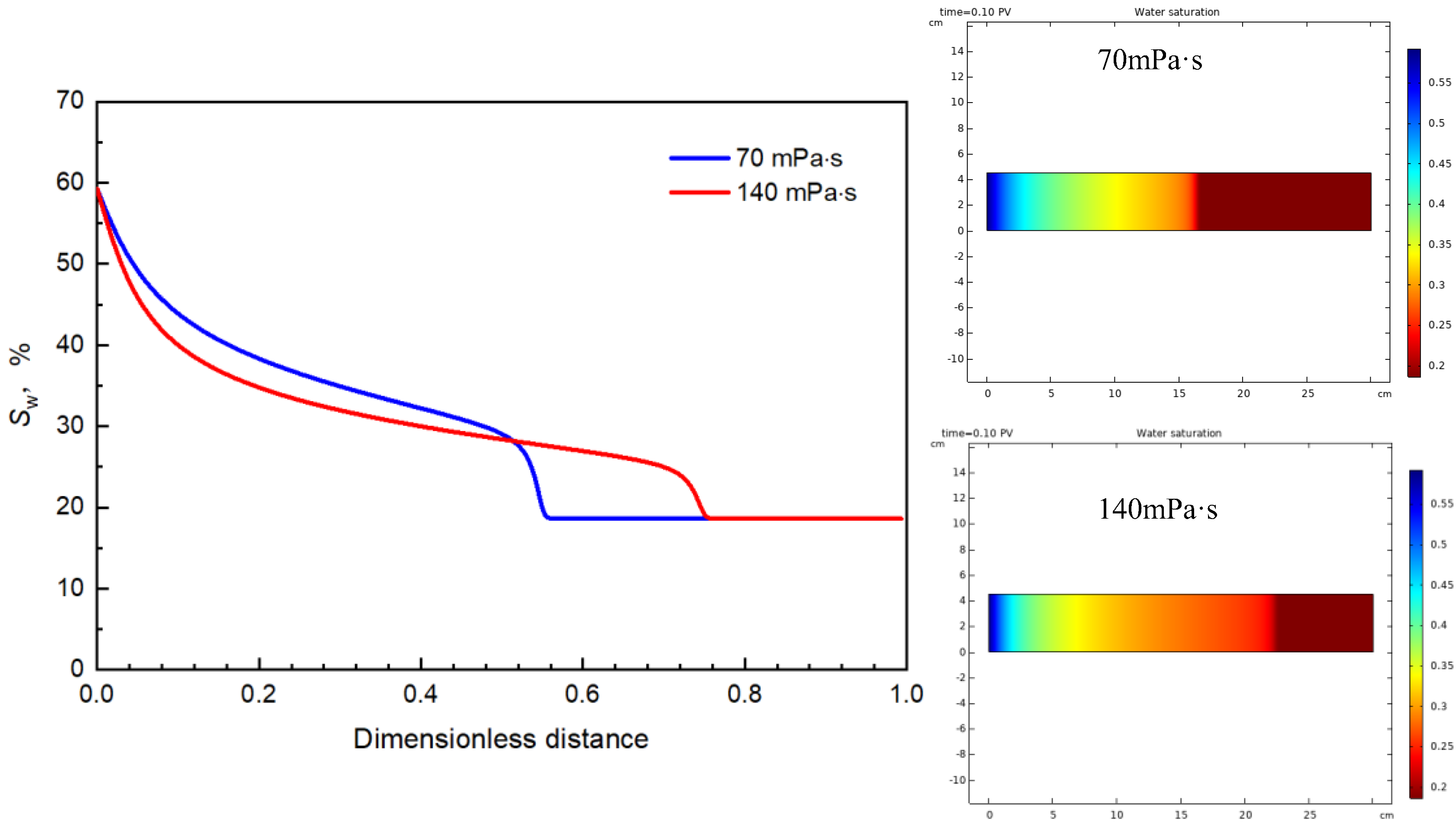
3.3.4. Effect of Increasing Oil Viscosity on the Displacement

In order to further analyze and verify the effect of the displacement agent viscosity on the oil displacement effect, the oil phase viscosity was increased from 70 mPa·s to 140 mPa·s on the basis of the constant water-oil viscosity ratio, and the displacement process was simulated.

At an injection time of 0.1 PV, the water saturation distribution along the flow was compared under different oil phase viscosity conditions during water flooding, as shown in Figure 21.

When the oil phase viscosity was increased, the water phase inrush speed became relatively fast during the water flooding. Before the breakthrough, the front edge of the water flooding was closer to the outlet at the same displacement time. At the same time, the sweep range of the water flooding was reduced, making the water saturation along the flow near the inlet end low.

The water saturation distribution along the flow under different water-oil viscosity ratio conditions at an injection time of 0.3 PV is shown in Figure 22.

Compared with the case in which the oil phase viscosity is 70 mPa·s, the water saturation decreasing distance is longer and the degree of reduction is greater. Similar to the situation in which the oil phase viscosity is 70 mPa·s, when the water-oil viscosity ratio exceeds 0.4, there is basically no great change in the decreasing section of water saturation; that is, the displacement effect will not increase, indicating that the optimal water-oil viscosity ratio still cannot exceed 0.4 under this condition.

The results of this study can clearly understand the action process of polymer flooding, so that during the selection of polymer solution, a more specific and reasonable concentration of polymer solution can be selected to avoid too high (high injection pressure) or too low (poor displacement effect) concentration and improve the application effect of polymer flooding.

4. Summary and Conclusions

Based on the Buckley-Leverett theory, this study established a one-dimensional displacement model and a simulation method that could obtain the change in water saturation along the flow. The research results revealed the polymer solution action process in enhancing oil recovery during displacement:

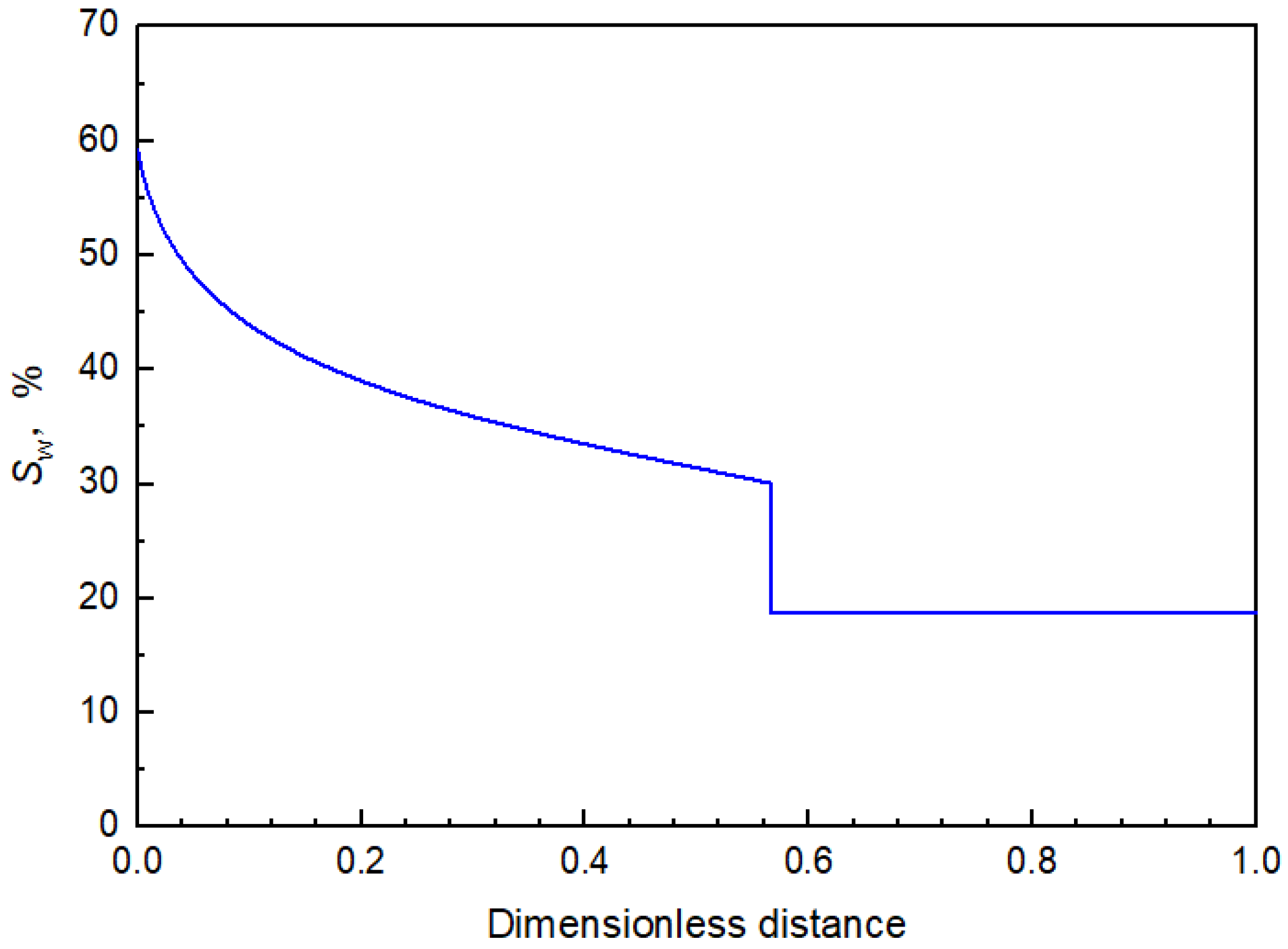
• The mobility control of polymer solution promotes oil phase accumulation, resulting in the decrease in water saturation along the flow, when the polymer solution viscosity increases, the water saturation decreasing region and the decreasing degree also increase.
• The viscosity of the polymer solution has an optimal value. When it reaches this value, the water cut will be reduced to the limit value under the action of the polymer solution. When the viscosity is further increased, the injection pressure is further increased, but the displacement effect will not change greatly.
• When the water-oil viscosity ratio increased from 0.1 to 0.6, oil viscosity of 70 mPa·s and 140 mPa·s have similar polymer solution displacement laws, and the optimal water-oil viscosity ratio under the two oil viscosity conditions is 0.4.

However, this study only investigated from the perspective of viscosity, and the results obtained without the consideration of other factors can be used as a reference. In further research, more polymer solution performance parameters can be added to the model to ensure a more accurate application range of model results.

References

1. Shah, A.; Fishwick, R.; Wood, J.; Leeke, G.; Rigby, S.; Greaves, M. A review of novel techniques for heavy oil and bitumen extraction and upgrading. Energy Environ. Sci. 2010, 3, 700–714. [Google Scholar] [CrossRef]
2. Mai, A.; Bryan, J.; Goodarzi, N.; Kantzas, A. Insights into Non-Thermal Recovery of Heavy Oil. J. Can. Pet. Technol. 2009, 48, 27–35. [Google Scholar] [CrossRef]
3. Chen, Z.; Zhao, X.; Wang, Z.; Fu, M. A comparative study of inorganic alkaline/polymer flooding and organic alkaline/polymer flooding for enhanced heavy oil recovery. Colloids Surf. A Physicochem. Eng. Asp. 2015, 469, 150–157. [Google Scholar] [CrossRef]
4. Khalilinezhad, S.S.; Hashemi, A.; Mobaraki, S.; Zakavi, M.; Jarrahian, K. Experimental Analysis and Numerical Modeling of Polymer Flooding in Heavy Oil Recovery Enhancement: A Pore-Level Investigation. Arab. J. Sci. Eng. 2019, 44, 10447–10465. [Google Scholar] [CrossRef]
5. Mohammadi, S.; Masihi, M.; Ghazanfari, M. Characterizing the Role of Shale Geometry and Connate Water Saturation on Performance of Polymer Flooding in Heavy Oil Reservoirs: Experimental Observations and Numerical Simulations. Transp. Porous Media 2012, 91, 973–998. [Google Scholar] [CrossRef]
6. Lie, K.A.; Nilsen, H.M.; Rasmussen, A.F.; Raynaud, X. Fast simulation of polymer injection in heavy-oil reservoirs on the basis of topological sorting and sequential splitting. SPE Journal 2014, 19, 991–1004. [Google Scholar] [CrossRef]
7. Xin, X.; Yu, G.; Chen, Z.; Wu, K.; Dong, X.; Zhu, Z. Effect of Non-Newtonian Flow on Polymer Flooding in Heavy Oil Reservoirs. Polymers 2018, 10, 1225. [Google Scholar] [CrossRef] [Green Version]
8. Shi, L.-T.; Zhu, S.; Zhang, J.; Wang, S.-X.; Xue, X.-S.; Zhou, W.; Ye, Z.-B. Research into polymer injection timing for Bohai heavy oil reservoirs. Pet. Sci. 2015, 12, 129–134. [Google Scholar] [CrossRef] [Green Version]
9. Li, Z.; Hou, J.; Liu, W.; Liu, Y. Multi-molecular mixed polymer flooding for heavy oil recovery. J. Dispers. Sci. Technol. 2022, 43, 1700–1708. [Google Scholar] [CrossRef]
10. Pei, H.; Zhang, G.; Ge, J.; Zhang, L.; Wang, H. Effect of polymer on the interaction of alkali with heavy oil and its use in improving oil recovery. Colloids Surf. A: Physicochem. Eng. Asp. 2014, 446, 57–64. [Google Scholar] [CrossRef]
11. Wassmuth, F.; Arnold, W.; Green, K.; Cameron, N. Polymer Flood Application to Improve Heavy Oil Recovery at East Bodo. J. Can. Pet. Technol. 2009, 48, 55–61. [Google Scholar] [CrossRef] [Green Version]
12. Asghari, K.; Nakutnyy, P. Experimental Results of Polymer Flooding of Heavy Oil Reservoirs. In Proceedings of the Canadian International Petroleum Conference, Calgary, Alberta, 17–19 June 2008. [Google Scholar] [CrossRef]
13. Guo, H. How to Select Polymer Molecular Weight and Concentration to Avoid Blocking in Polymer Flooding? In Proceedings of the SPE Symposium: Production Enhancement and Cost Optimisation, Kuala Lumpur, Malaysia, 7–8 November 2017. [Google Scholar] [CrossRef]
14. Delamaide, E.; Zaitoun, A.; Renard, G.; Tabary, R. Pelican Lake Field: First Successful Application of Polymer Flooding in a Heavy-Oil Reservoir. SPE Reserv. Eval. Eng. 2014, 17, 340–354. [Google Scholar] [CrossRef]
15. Demin, W.; Gang, W.; Huifen, X. Large Scale High Viscous-Elastic Fluid Flooding in the Field Achieves High Recoveries. In Proceedings of the SPE Enhanced Oil Recovery Conference, Kuala Lumpur, Malaysia, 19–20 July 2011. [Google Scholar] [CrossRef]
16. Seright, R.S. How Much Polymer Should Be Injected During a Polymer Flood? Review of Previous and Current Practices. SPE J. 2016, 22, 1–18. [Google Scholar] [CrossRef]
17. Seright, R.S.; Wang, D.; Lerner, N.; Nguyen, A.; Sabid, J.; Tochor, R. Can 25-cp Polymer Solution Efficiently Displace 1600-cp Oil During Polymer Flooding? SPE J. 2018, 23, 2260–2278. [Google Scholar] [CrossRef]
18. Levitt, D.; Jouenne, S.; Bondino, I.; Santanach-Carreras, E.; Bourrel, M. Polymer Flooding of Heavy Oil Under Adverse Mobility Conditions. In Proceedings of the SPE Enhanced Oil Recovery Conference, Kuala Lumpur, Malaysia, 2–4 July 2013. [Google Scholar] [CrossRef]
19. Wang, J.; Dong, M. Optimum effective viscosity of polymer solution for improving heavy oil recovery. J. Pet. Sci. Eng. 2009, 67, 155–158. [Google Scholar] [CrossRef]
20. Wang, J.; Dong, M. A Laboratory Study of Polymer Flooding for Improving Heavy Oil Recovery. In Proceedings of the Canadian International Petroleum Conference, Calgary, Alberta, 12–14 June 2007. [Google Scholar] [CrossRef]
21. Guo, Z.; Dong, M.; Chen, Z.; Yao, J. A fast and effective method to evaluate the polymer flooding potential for heavy oil reservoirs in Western Canada. J. Pet. Sci. Eng. 2013, 112, 335–340. [Google Scholar] [CrossRef]
22. Guo, Z.; Dong, M.; Chen, Z.; Yao, J. Dominant Scaling Groups of Polymer Flooding for Enhanced Heavy Oil Recovery. Ind. Eng. Chem. Res. 2013, 52, 911–921. [Google Scholar] [CrossRef]
23. Olayiwola, S.O.; Dejam, M. Comprehensive experimental study on the effect of silica nanoparticles on the oil recovery during alternating injection with low salinity water and surfactant into carbonate reservoirs. J. Mol. Liq. 2021, 325, 115178. [Google Scholar] [CrossRef]
24. Zhu, S.; Shi, L.; Wang, X.; Liu, C.; Xue, X.; Ye, Z. Investigation into mobility control mechanisms by polymer flooding in offshore high-permeable heavy oil reservoir. Energy Sources Part A Recover. Util. Environ. Eff. 2020, 1–14. [Google Scholar] [CrossRef]
25. Manichand, R.N.; Mogollon, J.L.; Bergwijn, S.S.; Graanoogst, F.; Ramdajal, R. Preliminary Assessment of Tambaredjo Heavy Oilfield Polymer Flooding Pilot Test. In Proceedings of the SPE Latin American and Caribbean Petroleum Engineering Conference, Lima, Peru, 1–3 December 2010. [Google Scholar] [CrossRef]
26. Gao, C. Scientific research and field applications of polymer flooding in heavy oil recovery. J. Pet. Explor. Prod. Technol. 2011, 1, 65–70. [Google Scholar] [CrossRef] [Green Version]
27. Ameli, F.; Moghbeli, M.R.; Alashkar, A. On the effect of salinity and nano-particles on polymer flooding in a heterogeneous porous media: Experimental and modeling approaches. J. Pet. Sci. Eng. 2019, 174, 1152–1168. [Google Scholar] [CrossRef]
28. Amiri, H.A.; Hamouda, A. Pore-scale modeling of non-isothermal two phase flow in 2D porous media: Influences of viscosity, capillarity, wettability and heterogeneity. Int. J. Multiph. Flow 2014, 61, 14–27. [Google Scholar] [CrossRef]
29. Afzali, S.; Zendehboudi, S.; Mohammadzadeh, O.; Rezaei, N. Hybrid mathematical modelling of three-phase flow in porous media: Application to water-alternating-gas injection. J. Nat. Gas Sci. Eng. 2021, 94, 103966. [Google Scholar] [CrossRef]
30. Honarpour, M.; Mahmood, S. Relative-Permeability Measurements: An Overview. J. Pet. Technol. 1988, 40, 963–966. [Google Scholar] [CrossRef]
31. Johnson, E.; Bossler, D.; Bossler, V.N. Calculation of Relative Permeability from Displacement Experiments. Trans. AIME 1959, 216, 370–372. [Google Scholar] [CrossRef]
32. Huang, Y.; Liu, F.; Yang, Z. Mass transfer of complex chemical fluids in porous media. Chin. J. Theor. Appl. Mech. 2002, 34, 256–260. (In Chinese) [Google Scholar]
Figure 1. Schematic of the research process.
Energies 15 09473 g001
Figure 2. The experimental flowchart.
Energies 15 09473 g002
Figure 3. Schematic diagram of the homogeneous model simulation of displacement.
Energies 15 09473 g003
Figure 4. Schematic diagram of water saturation distribution along the flow.
Energies 15 09473 g004
Figure 5. The oil-water relative permeability curve.
Energies 15 09473 g005
Figure 6. The curve of the water cut changing with water saturation.
Energies 15 09473 g006
Figure 7. The distribution of water saturation along the way at 0.11 PV injection time.
Energies 15 09473 g007
Figure 8. Comparison of water saturation distribution along the flow.
Energies 15 09473 g008
Figure 9. Comparison of water saturation along the flow under different densified grid conditions.
Energies 15 09473 g009
Figure 10. Water saturation under different injection time of water flooding.
Energies 15 09473 g010
Figure 11. Water saturation distribution along the flow during water flooding.
Energies 15 09473 g011
Figure 12. The water cut change at the outlet end.
Energies 15 09473 g012
Figure 13. Water saturation at different injection times when water-oil viscosity ratio is 0.1.
Energies 15 09473 g013
Figure 14. Comparison of water saturation distribution along the flow when the displacement time is 0.3 PV.
Energies 15 09473 g014
Figure 15. Concentration of polymer solution along the flow.
Energies 15 09473 g015
Figure 16. Water saturation change along the flow when water-oil viscosity ratio is 0.1.
Energies 15 09473 g016
Figure 17. Comparison of water saturation distribution along the flow under different water-oil viscosity ratio conditions.
Energies 15 09473 g017
Figure 18. The change curves of the water cut under different viscosity conditions.
Energies 15 09473 g018
Figure 19. Oil recovery under different water-oil viscosity ratios.
Energies 15 09473 g019
Figure 20. The injection pressure under different viscosity conditions.
Energies 15 09473 g020
Figure 21. Water saturation distribution along the flow under different oil phase viscosity conditions.
Energies 15 09473 g021
Figure 22. Comparison of water saturation distribution along the flow under different water-oil viscosity ratio conditions.
Energies 15 09473 g022