Analysis on Position Estimation Error of Sensorless Control Based on Square-Wave Injection for SynRM Caused by Dead-Time Harmonic Current

Abstract

Sensorless control based on high-frequency square-wave voltage injection (HFSVI) is one of the most common sensorless control methods for synchronous reluctance motors (SynRMs). However, the injection frequency for SynRMs cannot be too high due to various factors. As the injection frequency decreases, the dead-time harmonic current will greatly affect the separation of high frequency signals. This paper analyzes the effect of dead-time harmonic current on the HFSVI-based sensorless control performance of SynRMs and proposes a source of position estimation error. Then, a dead-time compensation method suitable for filter-free HFSVI is proposed. It can estimate current vector spatial orientation without any low-pass filters (LPFs) and effectively compensate the impact of dead-time setting. The correctness of the theoretical analysis and the feasibility of the proposed methods in this paper are verified by experiments.

1. Introduction

Synchronous reluctance motors (SynRMs) have increasingly become a new research trend in industrial applications and electric vehicles due to their high reliability, high robustness and low cost [1]. Additionally, rare-earth permanent magnets materials used in PMSMs can be largely avoided, which make SynRMs a resource-saving and low-cost alternative for other motors [2]. However, accurate speed and rotor position are necessary for a modern control system of SynRMs. The use of sensors makes the system complex and expensive, and thus reduces the advantages of SynRMs [3]. Therefore, sensorless control is desired.

At present, a variety of sensorless control methods for SynRMs have been proposed successively. These methods can be divided into two main kinds [4]: model methods based on the SynRM basic frequency model, and high-frequency voltage injection methods. Model methods need the back electromotive force (EMF) which is related to the rotor speed and susceptible to noise [5]. Thus, these methods are widely used in high-speed and medium-speed conditions [6]. In low-speed or startup conditions, the back EMF is too small to observe so the control methods based on high-frequency voltage injection are widely used [7]. It can be divided into rotating high-frequency voltage injection methods and pulsating high-frequency voltage injection methods in principle [8]. The pulse injection method has gradually become the mainstream injection method due to more accurate observation performance and simple signal separation. At present, an eye-catching technical path is the filter-free high-frequency square-wave voltage injection (HFSVI) method [9]. These methods inject HF square-wave signals into stators to generate triangular wave response current, and then estimate the rotor position via response current signals [10,11]. Compared with previous sensorless control methods, these methods have many excellent characteristics, such as no need to use filters, high system bandwidth, the low computational load of the controller, and so on [12,13]. However, they are still affected by several factors such as the non-linear characteristics of the inverters [14], which will cause various sources of position estimation error [15].

Based on different ideas, there has been some research on error analysis of filter-free HFSVI. In [16], cross-coupling of magnetic circuits is considered one of the main sources of position estimation error. In [17], the effect of semiconductor switching tubes voltage drop on the accuracy of HFSVI is analyzed in detail. Additionally, several studies have suggested that the non-linear effect of the inverter will distort the injection voltage signal [18]. Thus, several modified HFSVI methods have been proposed [19]. However, most of these studies are based on PMSM, considering the error analysis of injection frequency conditions above 10 kHz, and generally only discuss the effect of injection high-frequency voltage distortion. In practical applications, some motors have large inductance, especially SynRMs with high torque [20], sometimes the response current will approach the lower detection limit of current sensors. In this case, the injection frequency can be reduced to increase the amplitude of high-frequency response current and the switching frequency is still maintained at a higher frequency to achieve high dynamic response performance. However, at lower frequency injection conditions, the harmonic current and even the fundamental current will have a greater impact on the accuracy of rotor position estimation, but there are few studies on this.

In this paper, the error of position estimation caused by the harmonic current caused by dead-time effect are analyzed when the filter-free HFSVI method is used. In contrast to previous studies, a new source of error for filter-free square wave injection at lower injection frequencies is proposed by qualitative analysis of current components. This paper then presents a dead-time effect compensation method suitable for the SynRM sensorless control system based on filter-free square-wave voltage injection. This method filters out the high-frequency signal by a filter-free signal separation method. This paper also proposes compensating voltage sector lag angles to reduce the influence of current space angle ripple on compensation. Compared with the other methods, this method can achieve acceptable accuracy in current vector spatial orientation without any low-pass filters and effectively compensate for dead-time effects.

This paper is organized as follows: the model of SynRMs and filter-free HFSVI methods is presented in Section 2; analysis of error caused by dead time effect harmonic current is presented in Section 3; current polarity detection and dead-time effect compensation for filter-free square-wave injection method are presented in Section 4; experiment results are presented in Section 5; conclusions are finally provided in Section 6.

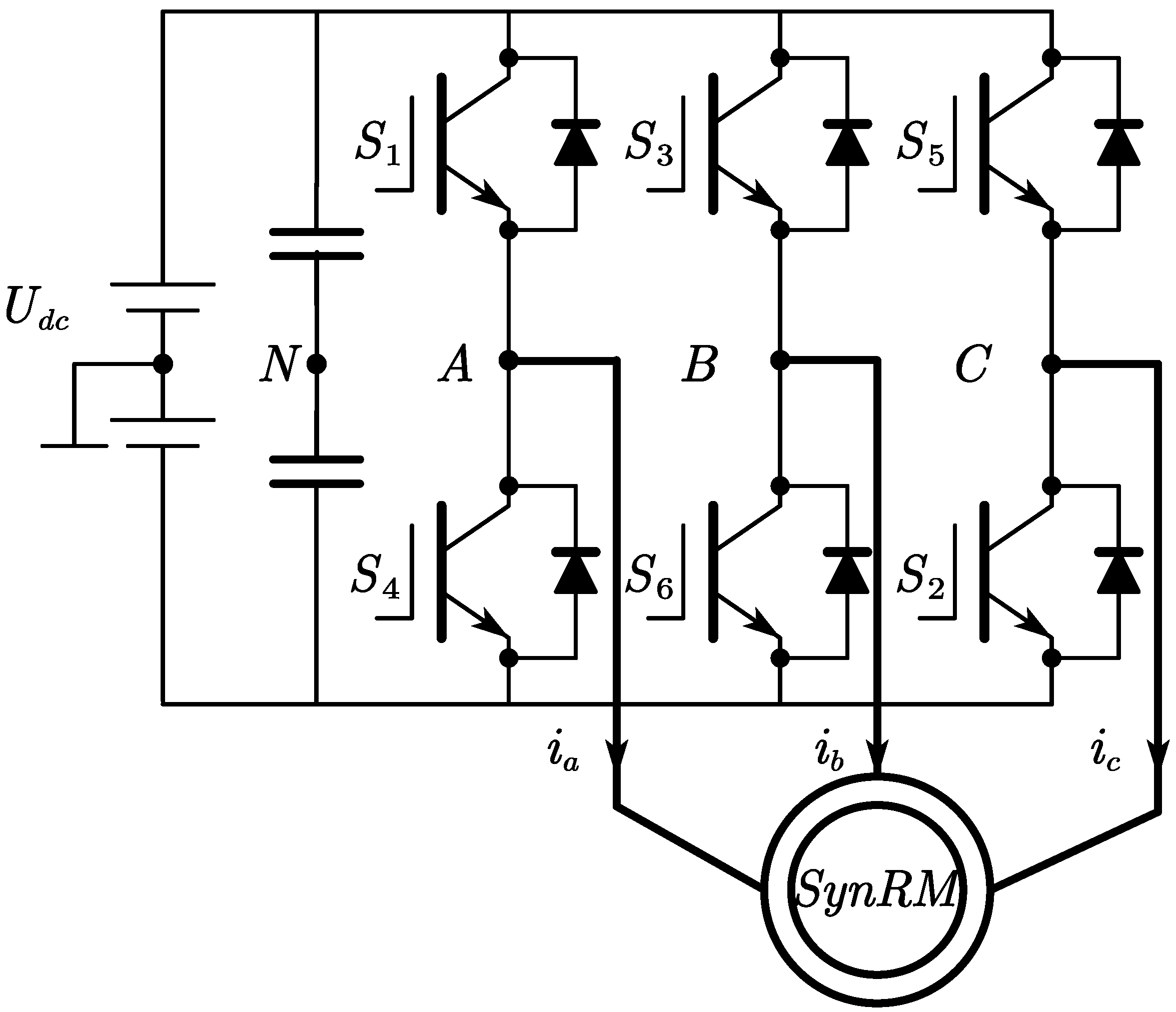
2. Sensorless Control Based on Filter-Free Square-Wave Voltage Injection

2.1. The High-Frequency Equivalent Model of SynRM

The voltage and flux linkage equivalent mathematical model of the SynRM in the synchronous reference frame can be shown in (1):

$$\left[\begin{array}{c}{u}_d\\ u_q\end{array}\right]=\left[\begin{array}{cc}{R}_{\mathrm{s}}+L_{d}p& -{\omega }_e{L}_q\\ {\omega }_e{L}_d& R_s+L_{q}p\end{array}\right]\left[\begin{array}{c}{i}_d\\ i_q\end{array}\right]$$

(1)

where u_d and u_q represent the d-axis and q-axis voltages, respectively, while i_d and i_q are the d-axis and q-axis current, respectively; ω_e is the electrical rotor speed (rad/s); R_s is the winding resistance; p is a differential operator. When the frequency of injection signal is high enough, the voltage drop on the stator resistor and back-EMF are too small, so R_s and ω_e can be ignored. Finally, (1) can be simplified to (2):

$$\left[\begin{array}{c}{u}_{dh}\\ u_{qh}\end{array}\right]=\left[\begin{array}{cc}{L}_{d}p& 0\\ 0& L_{q}p\end{array}\right]\left[\begin{array}{c}{i}_{dh}\\ i_{qh}\end{array}\right]$$

(2)

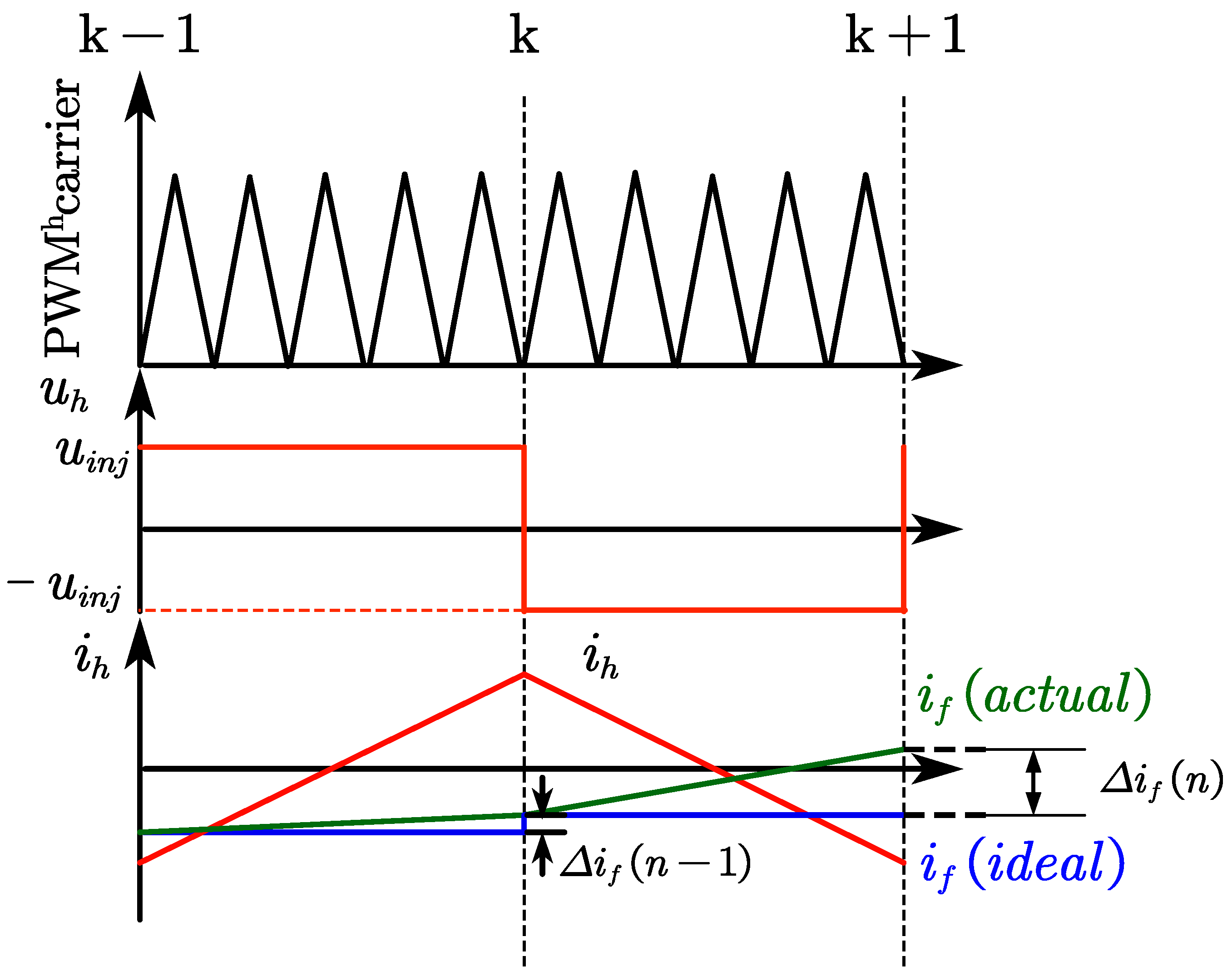
2.2. Sensorless Control Based on Filter-Free Square Voltage Injection

The use of LPFs will cause additional chip computing load, reduce the dynamic performance of the system, and cause phase error. This is one of the main reasons why the filter-free HFSVI method is favored by more and more researchers. When the injected signal is in the form of (3), transform (2) from the estimated dq frame to αβ frame. In the αβ static frame, the HF current response can be obtained by (4):

$$\left[\begin{array}{c}{u}_{dh}\\ u_{qh}\end{array}\right]=\left[\begin{array}{c}{U}_{inj}{(-1)}^k\\ 0\end{array}\right]$$

(3)

$$\left[\begin{array}{c}p{i}_{\alpha h}\\ p{i}_{\beta h}\end{array}\right]=T({\theta }_e)\left[\begin{array}{c}p{i}_{dh}\\ p{i}_{qh}\end{array}\right]=T({\theta }_e){\left[\begin{array}{cc}{L}_d& 0\\ 0& L_q\end{array}\right]}^{-1}T({\tilde{\theta }}_e-{\theta }_e)\left[\begin{array}{c}{u}_{dh}\\ u_{qh}\end{array}\right]$$

(4)

In (3), $U_{inj}$ is the amplitude of the injected signal, $T({\theta }_e)$, $T({\tilde{\theta }}_e-{\theta }_e)$ are coordinate system transformation matrix, similarly to the form of (5), ${\tilde{\theta }}_e$ is the estimation electrical angle.

$$T(\theta )=\left[\begin{array}{cc}\cos \theta & -\sin \theta \\ \sin \theta & \cos \theta \end{array}\right]$$

(5)

Extracting the envelope signal of the current response, the response signal containing position information can be obtained, shown as (6), in which $\Delta {\theta }_e$ means the estimated angular error:

$$\left[\begin{array}{c}{I}_{\alpha h}\\ I_{\beta h}\end{array}\right]=\frac{U_{inj}}{2f_h{L}_d{L}_q}\left[\begin{array}{c}(L_d+L_q)\cos {\tilde{\theta }}_e-(L_d-L_q)\cos ({\theta }_e+\Delta {\theta }_e)\\ (L_d+L_q)\sin {\tilde{\theta }}_e-(L_d-L_q)\sin ({\theta }_e+\Delta {\theta }_e)\end{array}\right]$$

(6)

Under low-speed or middle-speed conditions, the frequency of the injected high-frequency square wave signal is usually much greater than the frequency of the fundamental frequency current. Thus, the fundamental frequency current can be considered as basically unchanged in a square wave period. When the sampling frequency is kept at half of the injection frequency, the HF response current has symmetry, with equal amplitude and opposite polarity at adjacent sampling times. Therefore, the high-frequency response current signal can be simply separated without LPFs [21]. The analysis above can be more clearly represented by Figure 1.

As shown in Figure 1, αβ-axis HF response current can be simply calculated by (7). In (7), k means the kth sampling, k − 1 represents the k − 1th sampling and the subscript h represents the high-frequency quantity:

$$\{\begin{array}{c}{i}_{dh}(k)=\frac{i_d(k)-i_d(k-1)}{2}\\ i_{qh}(k)=\frac{i_q(k)-i_q(k-1)}{2}\end{array}$$

(7)

Convert high-frequency current signal obtained by (7) to αβ coordinate, $I_{\alpha h}$ and $I_{\beta h}$ can be obtained by using an envelope extractor. Thus, the values of high frequency or base frequency current at any sampling time can be obtained by two adjacent samples. The filter-free signal separation method greatly improves the system response speed, reduces the phase error, and significantly improves the control performance. As shown in Figure 2, the estimated position information can be further extracted by position observer, such as the phase-locked loop [21].

This method is mature and robust. Under ideal conditions, the observation error is relatively small. However, there are still some defects in practical engineering applications, especially in the case of setting the dead zone of switching devices, the error will be multiplied. The next section will analyze and improve this.

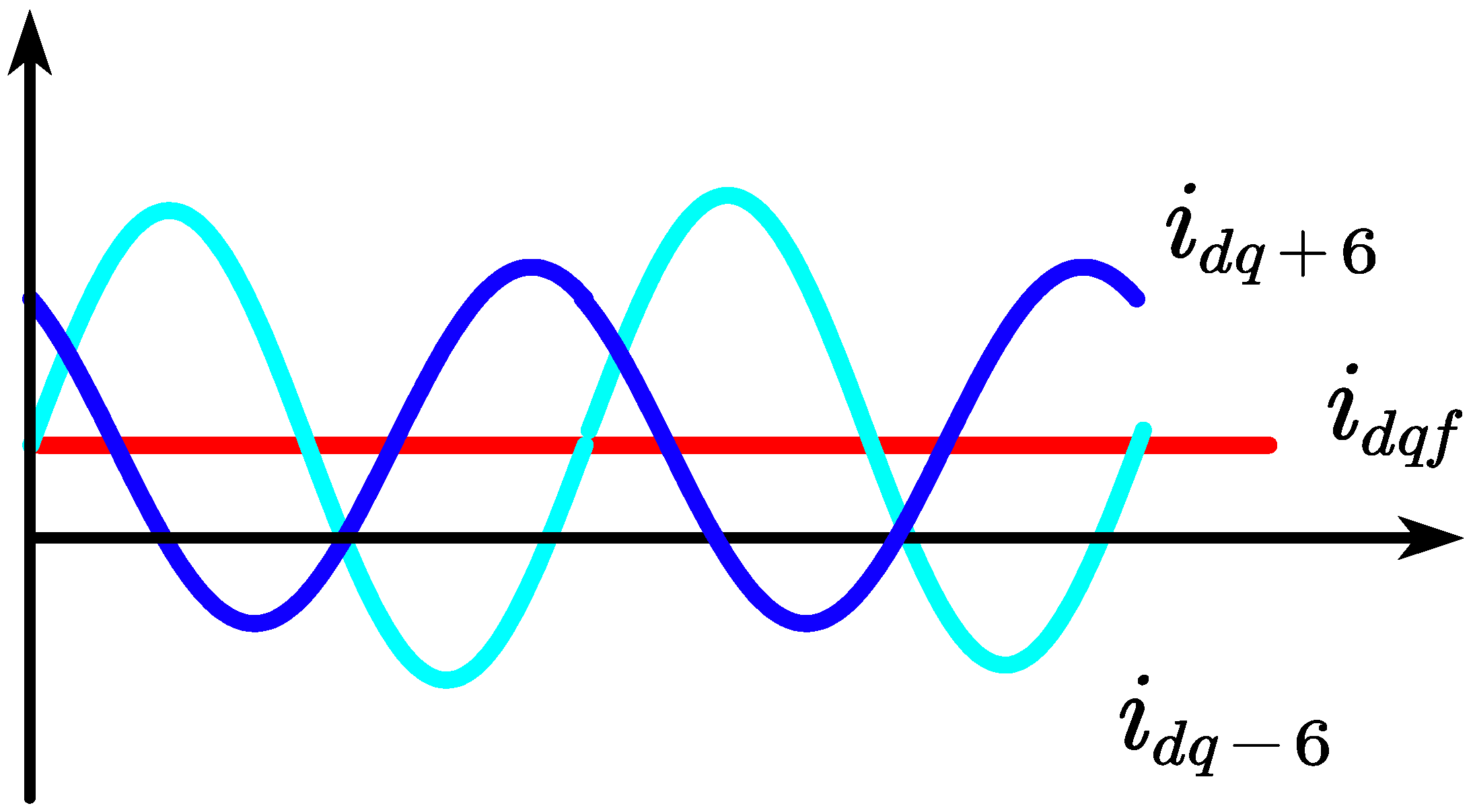
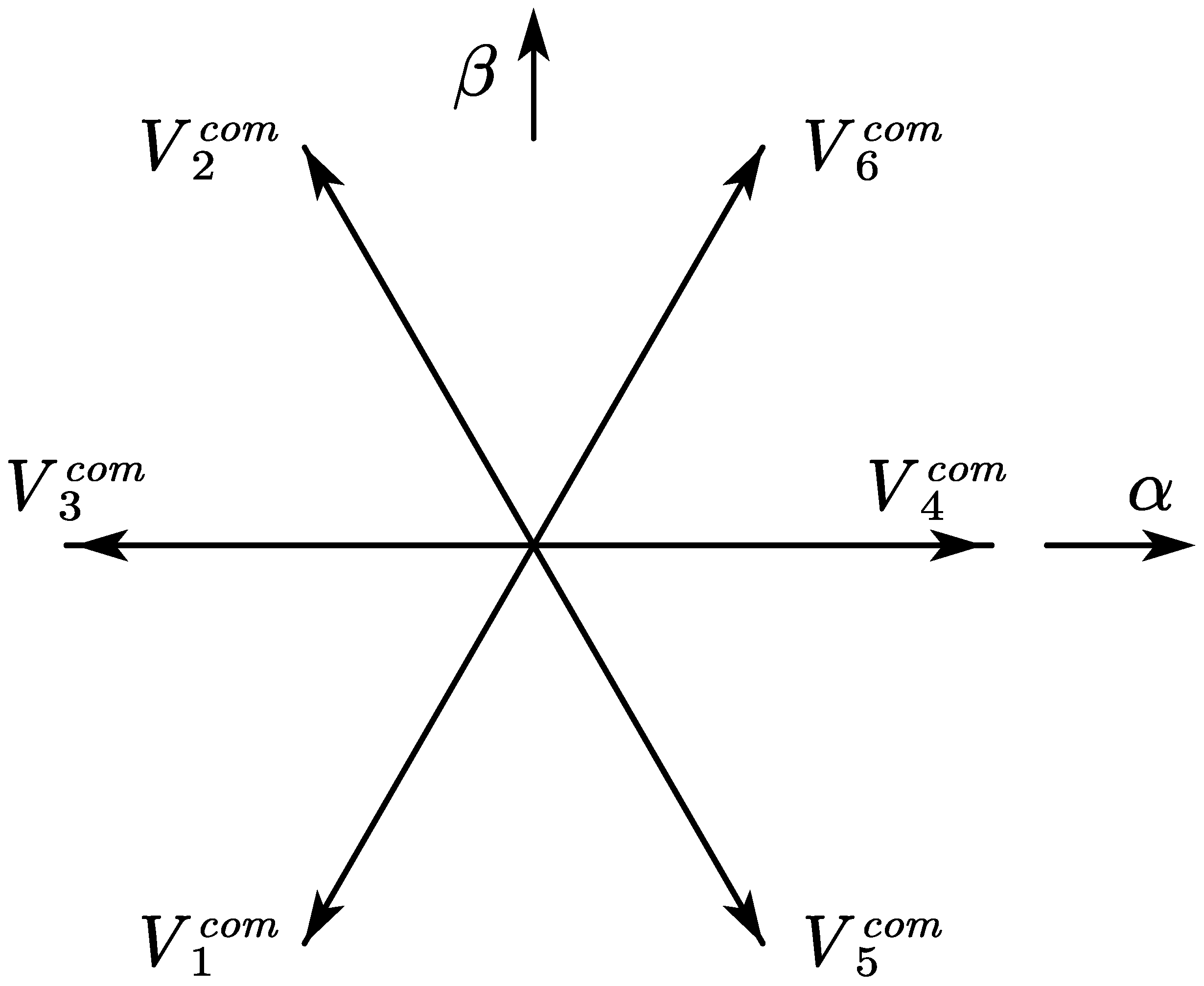
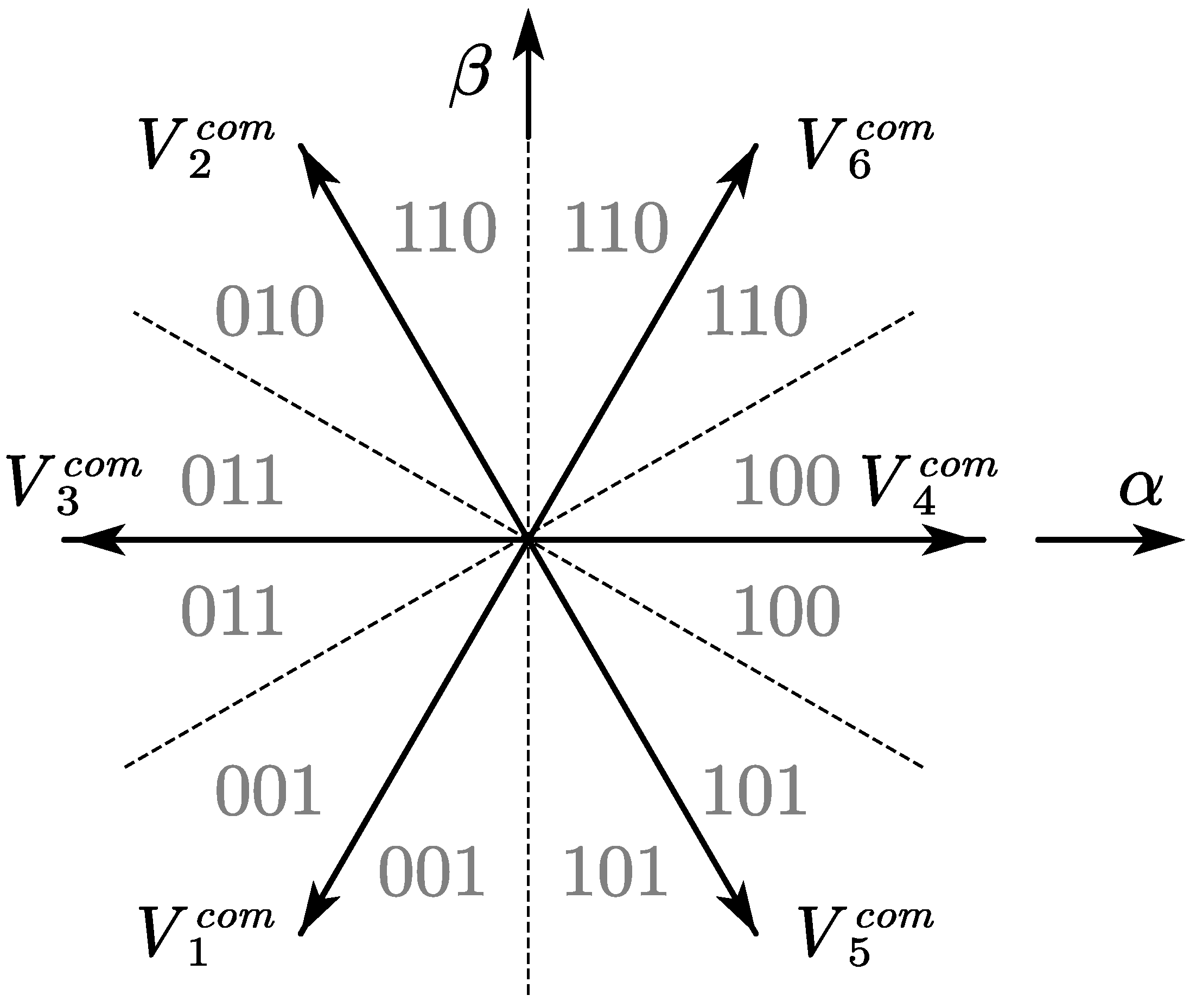
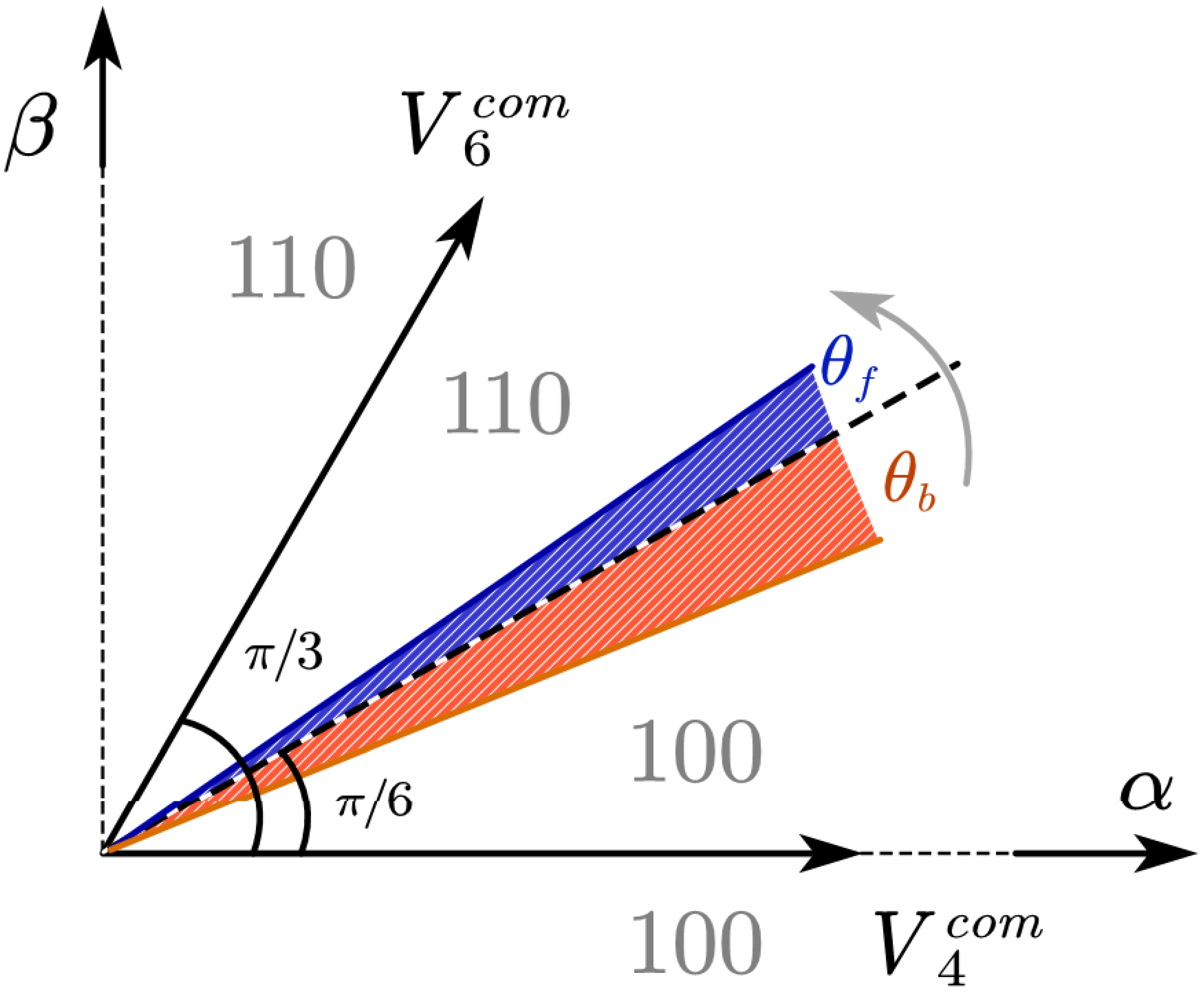
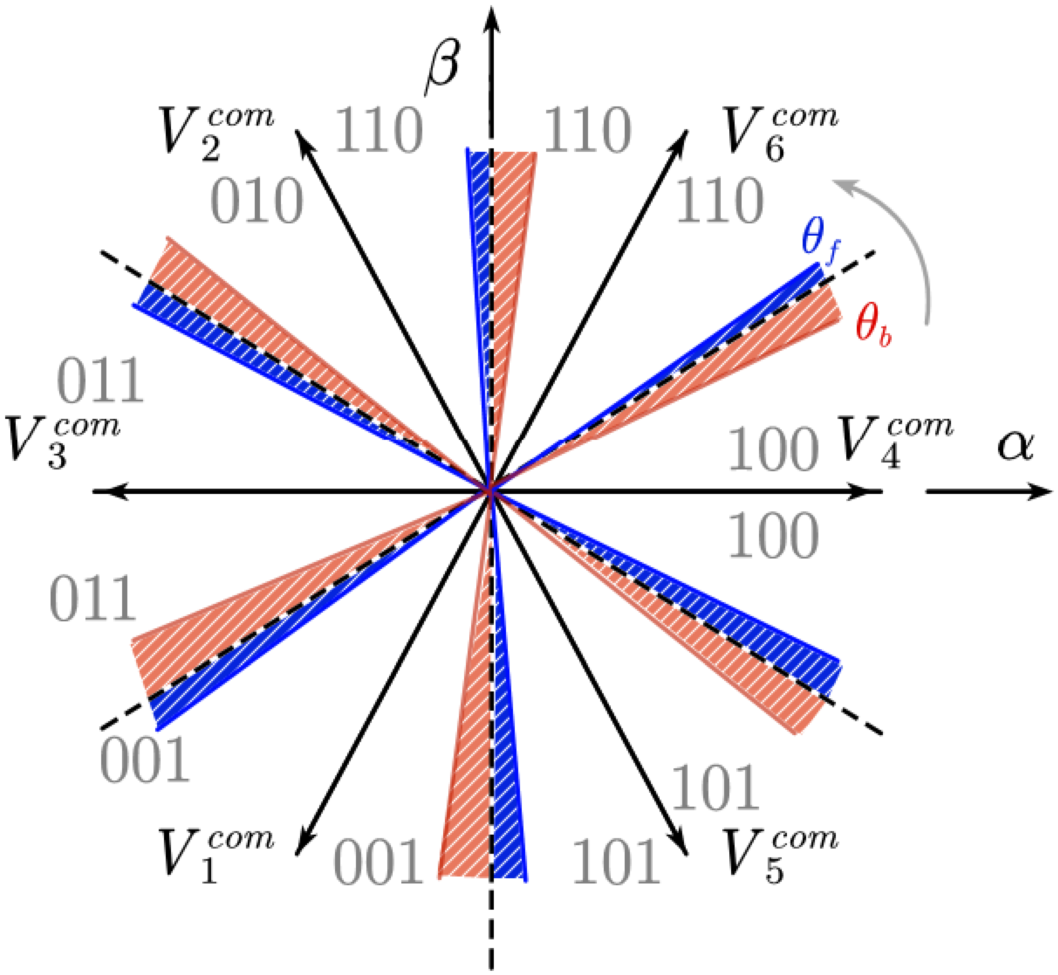
3. Analysis of Error Caused by Dead-Time Effect Harmonic Current

A classic three-phase PWM voltage-source inverter based on insulated-gate bipolar transistors (IGBT) is shown in Figure 3. Its load is a SynRM, which can be considered as a resistive-inductive load. When using an inverter in practice, due to the limitation of physical properties of switching devices (such as on–off time, etc.), in order to avoid failure and damage to equipment, it is necessary to set a dead-time. Thus, the PWM signals of a pair of bridge arms of the inverter will not be strictly complementary, which will lead to output voltage distortion.

The dead-time effect will cause a series of distorted voltage pulses, and the vector direction of the pulse is related to the polarity of the phase current. According to the voltage equivalent principle, these voltage pulses can be equivalent to a 180° conducting square wave, shown in Figure 4. Since the three-phase currents differ by 120° from each other, six error voltage vectors are formed in the motor winding [22].

The direction of the error voltage vector is determined by the polarity of the phase current. Define the phase current which flows into the motor winding as the positive polarity and mark the positive polarity as 1, the negative polarity as 0. Arrange current polarity in A, B, and C phases, the combined number is the corresponding error voltage vector. For example, when the A-phase current is positive and the B, C-phase current is negative, it corresponds to 100, that is, $\Delta V_4$.

Taking A-phase as an example, the phase voltage error caused by the dead-time effect in a switching cycle is defined as $\Delta V_4$, given by (8) and (9):

$$V_d=-f_s(T_d+T_{on}-T_{off})V_{dc}$$

(8)

$$\Delta V_A=V_{d}sgn\left(i_a\right)$$

(9)

where $T_d,T_{on},T_{off}$ are dead-time setting, on time and off time of the IGBT. $f_s$ is the switching frequency. $sgn\left(i_a\right)$ is the symbolic function of A-phase current; when the current is in the reference direction, its value is 1, otherwise it is −1.

The influence of dead time effect on other two phases is similar. Transform error voltage vectors into two-phase static reference frame (αβ frame) and synchronous reference frame (dq frame), and obtain the Fourier decomposition of them; then, (10) and (11) can be obtained:

$$\{\begin{array}{l}{U}_{\alpha e}=-\frac{4U_e}{\pi }\left(\sin {\omega }_{e}t+{\displaystyle \sum _{k=1}^{\infty }\frac{\sin [(6k-1){\omega }_{e}t]}{6k-1}+{\displaystyle \sum _{k=1}^{\infty }\frac{\sin [(6k+1){\omega }_{e}t]}{6k+1}}}\right)\hfill \\ U_{\beta e}=\frac{4U_e}{\pi }\left(\cos {\omega }_{e}t-{\displaystyle \sum _{k=1}^{\infty }\frac{\cos [(6k-1){\omega }_{e}t]}{6k-1}+{\displaystyle \sum _{k=1}^{\infty }\frac{\cos [(6k+1){\omega }_{e}t]}{6k+1}}}\right)\hfill \end{array}$$

(10)

$$\{\begin{array}{l}{U}_{de}=\frac{4U_e}{\pi }\left(\sin \phi -{\displaystyle \sum _{k=1}^{\infty }\frac{-\sin \left(-6k{\omega }_{e}t-\phi \right)}{6k-1}+{\displaystyle \sum _{k=1}^{\infty }\frac{-\sin \left(6k{\omega }_{e}t-\phi \right)}{6k+1}}}\right)\hfill \\ U_{qe}=\frac{4U_e}{\pi }\left(\cos \phi -{\displaystyle \sum _{k=1}^{\infty }\frac{\cos \left(-6k{\omega }_{e}t-\phi \right)}{6k-1}+{\displaystyle \sum _{k=1}^{\infty }\frac{\cos \left(6k{\omega }_{e}t-\phi \right)}{6k+1}}}\right)\hfill \end{array}$$

(11)

It is clear that the amplitude of harmonic voltage is inversely proportional to the harmonic order. Sensorless position estimation based on filter-free HF square-wave injection needs to obtain HF current signal in αβ frame. In αβ frame, the major harmonic components are 1st, 5th, and 7th order harmonics. The separation of high-frequency signals is carried out in dq frame, so ±6th order component is mainly considered. From (11) the steady-state dead-time effect current in dq frame can be provided by (12):

$$\{\begin{array}{l}{i}_{de}=\frac{4U_e}{\pi }\left(\frac{\sin \phi }{R}-\frac{-\sin \left(-6{\omega }_{e}t-\phi \right)}{5\sqrt{R^2+36{\omega }_e^2{L}_d^2}}+\frac{-\sin \left(6{\omega }_{e}t-\phi \right)}{7\sqrt{R^2+36{\omega }_e^2{L}_d^2}}\right)\hfill \\ i_{qe}=\frac{4U_e}{\pi }\left(\frac{\cos \phi }{R}-\frac{\cos \left(-6{\omega }_{e}t-\phi \right)}{5\sqrt{R^2+36{\omega }_e^2{L}_q^2}}+\frac{\cos \left(6{\omega }_{e}t-\phi \right)}{7\sqrt{R^2+36{\omega }_e^2{L}_q^2}}\right)\hfill \end{array}$$

(12)

The core assumption of the filter-free signal separation method is that when the HF current is separated within a sampling cycle, the change of fundamental current can be ignored. However, in practice, the frequency of injected voltage should not be too high. As shown in (13), $\Delta t$ is the sampling step which is generally set to half the injection frequency. If $L_d$ is large enough and $\Delta t$ is too small, the current signal will be too weak to be accurately detected, so the influence of instrument error and sampling step will be too significant to be ignored. Taking the accuracy of sampling points, chip computing load, and other factors into account, the injection frequency is generally lower than 5 kHz, or even reduced to 1 kHz in practice.

$$\left|i_{dh}(k)-i_{dh}(k-1)\right|=\frac{U_{inj}}{L_d}\Delta t$$

(13)

When the injection frequency decreases, although it is still small, the error caused by the change in harmonic current mentioned above has become a problem worthy of discussion. Taking any axis current as an example, the schematic diagrams of HF square-wave voltage, high-frequency response current, and fundamental wave current are shown in Figure 5.

The dq-axis current, other than the high-frequency response current, can be reasonably decomposed into (14):

$$\{\begin{array}{c}{i}_{dsum}(t)=A_f-A_{+6}\sin (6{\omega }_{e}t-\phi )+A_{-6}\sin (-6{\omega }_{e}t-\phi )\\ i_{qsum}(t)=B_f+B_{+6}\cos (6{\omega }_{e}t-\phi )-B_{-6}\cos (-6{\omega }_{e}t-\phi )\end{array}$$

(14)

As shown in Figure 6, $i_{dqf},i_{dq+6},i_{dq-6}$ are DC component, 6th and −6th harmonics of dq-axis current, respectively. $i_{other}$ is other components, including ripple current caused by the controller. This paper focuses on the influence of the dead-time effect current, so it mainly considers the influence of ±6^th harmonic current. Therefore, (14) is rewritten into the form of (15):

$$\{\begin{array}{c}{i}_{dsum}(t)=A_f-A_{+6}\sin (6{\omega }_{e}t-\phi )+A_{-6}\sin (-6{\omega }_{e}t-\phi )\\ i_{qsum}(t)=B_f+B_{+6}\cos (6{\omega }_{e}t-\phi )-B_{-6}\cos (-6{\omega }_{e}t-\phi )\end{array}$$

(15)

In (15), A/B and subscript number, respectively, represent the amplitudes of the fundamental current and harmonic components of different orders. Even the frequency of the 6th harmonic is still low enough relative to the injection frequency. Therefore, the change of current $\Delta i_{dq}(t)$ during the sampling step $\Delta t$ can be expressed as the product of the derivative of each current component at time t and the step time, shown as (15):

$$\{\begin{array}{c}\Delta i_d(t)=[-6A_{+6}\cos (6{\omega }_{e}t-\phi )-6A_{-6}\cos (-6{\omega }_{e}t-\phi )]{\omega }_e\Delta t\\ \Delta i_q(t)=[-6B_{+6}\sin (6{\omega }_{e}t-\phi )-6B_{-6}\cos (-6{\omega }_{e}t-\phi )]{\omega }_e\Delta t\end{array}$$

(16)

When the load is fixed, the faster the motor speed is, the greater the output electromagnetic torque is, so the current will increase. The SynRM has obvious magnetic circuit saturation and cross coupling, which makes the inductance of the dq-axis reduce. It is more obvious in the axis with more airgap.

According to (12) and (16), let $A_{+6}^1$ be the amplitude of the 6th harmonic current at electric angular velocity ${\omega }_{e1}$, $A_{+6}^2$ be the amplitude of the 6th harmonic current at ${\omega }_{e2}$. If ${\omega }_{e1}<{\omega }_{e2}$, then $A_{+6}^1{\omega }_{e1}<A_{+6}^2{\omega }_{e2}$. That means that the faster the rotor speed, the greater the current variation between sampling steps.

Come back to (7) with conclusions above. At the nth sampling time, the current signal obtained by processing the value of nth sampling and the (n − 1)th sampling is not entirely a high-frequency current signal. It also includes the variation of other current components during the sampling step, shown as Figure 7. Mark the (n − 1)th sampling time as t − △t, the nth sampling time as t, and rewrite (7) to (17).

$$\{\begin{array}{c}{i}_{dh}^{*}(n)=i_{dh}(n)+\Delta i_d(n-1)/2=i_{dh}(n)+i_{dhe}(n)\\ i_{qh}^{*}(n)=i_{qh}(n)+\Delta i_q(n-1)/2=i_{qh}(n)+i_{qhe}(n)\end{array}$$

(17)

In (17), $i_{dqh}(n)$ is the error of HF response current obtained by filter-free signal separation method at nth sampling time.

Converting (17) to αβ-frame can obtain (18). After the envelope detector, high-frequency current envelope and error signal for estimating the rotor position can be obtained, shown in (19):

$$\begin{array}{c}\left[\begin{array}{c}{i}_{\alpha h}^{*}(n)\\ i_{\beta h}^{*}(n)\end{array}\right]=T(\theta )\left[\begin{array}{c}{i}_{dh}^{*}(n)\\ i_{qh}^{*}(n)\end{array}\right]=\left[\begin{array}{c}{i}_{\alpha h}(n)\\ i_{\beta h}(n)\end{array}\right]+\left[\begin{array}{c}{i}_{\alpha he}(n)\\ i_{\beta he}(n)\end{array}\right]\\ \left[\begin{array}{c}{i}_{\alpha he}(n)\\ i_{\beta he}(n)\end{array}\right]=T({\theta }_e)\left[\begin{array}{c}{i}_{dhe}(n)\\ i_{qhe}(n)\end{array}\right]=\left[\begin{array}{c}\cos {\theta }_e{i}_{dhe}(n)-\sin {\theta }_e{i}_{qhe}(n)\\ \sin {\theta }_e{i}_{dhe}(n)+\cos {\theta }_e{i}_{qhe}(n)\end{array}\right]\end{array}$$

(18)

$$\left[\begin{array}{c}{I}_{\alpha h}^{*}(n)\\ I_{\beta h}^{*}(n)\end{array}\right]=\left[\begin{array}{c}{I}_{\alpha h}(n)\\ I_{\beta h}(n)\end{array}\right]+\mathrm{sgn}[u_{dh}(n)]\left[\begin{array}{c}{i}_{\alpha he}(n)\\ i_{\beta he}(n)\end{array}\right]$$

(19)

Compare (6) with (19), when using (6) and for vector cross multiplication, the input of position observer is $k·2\Delta {\theta }_e$, as shown in (20):

$$\{\begin{array}{l}-I_{\alpha h}\sin {\tilde{\theta }}_e+I_{\beta h}\cos {\tilde{\theta }}_e=k[\sin (2\Delta {\theta }_e)+\cos (2\Delta {\theta }_e)]\approx k·2\Delta {\theta }_e\hfill \\ k=\frac{U_{inj}(L_d-L_q)}{2f_h{L}_d{L}_q}\hfill \end{array}$$

(20)

However, when using (19), the inputs will change to (21):

$$\{\begin{array}{c}{I}_{\beta h}^{*}\cos {\tilde{\theta }}_e-I_{\alpha h}^{*}\sin {\tilde{\theta }}_e\approx 2k\Delta {\theta }_e+Error\\ Error=\mathrm{sgn}[u_{dh}(n)][i_{dhe}(n)\sin \Delta {\theta }_e+i_{qhe}(n)\cos \Delta {\theta }_e]\end{array}$$

(21)

According to (16), (17), and (21), the value of $i_{dqhe}(n)\Delta {\theta }_e$ changes periodically and the amplitude depends on the magnitude of the ±6-th harmonic current. Therefore, the higher the harmonic content, the greater the variation of current within the sampling steps, and the more significant the possible error of the sensorless rotor position estimation. In practice, with appropriate dead-time setting, the total harmonic distortion (THD) of stator current of an unloaded SynRM is between 20–40% [23]. However, the position error caused by it may lead to the deterioration of the controller performance, which will further increase $i_{dqhe}(n)$. In addition, due to the combined influence of multiple factors (such as magnet harmonic caused by auxiliary permanent magnet), the error may be multiplied compared with the ideal condition. Additionally, when the injection frequency decreases or the rotor speed increases, $i_{dqhe}(n)$ will also increase, and the error will be more significant.

4. Current Polarity Detection and Dead-Time Effect Compensation for Filter-Free Square-Wave Injection

4.1. Voltage Compensation Methods for Inverter

In order to reduce the error of the sensorless position estimation method based on filter free square wave injection caused by dead-time effects, dead-time compensation is desired. For SVPWM modulation methods, voltage compensation is commonly used. Generate vectors with the same size and opposite direction as the dead-time error voltage, so as to reduce the influence of dead-time effects, shown in Figure 8.

The compensated voltage vector is represented by $V_i^{com}$, the subscript I means the error voltage vector serial number. Then, $V_i^{com}$ can be expressed as (22):

$$\{\begin{array}{c}{V}_i^{com}=-\Delta V_i\\ \left|V_i^{com}\right|=f_s(T_d+T_{on}-T_{off})V_{dc}\end{array}$$

(22)

Project $V_i^{com}$ to the α-axis and the β-axis, respectively, and αβ-axis component can be obtained. Take $V_4^{com}$, which is the compensated vector for $\Delta V_4$, as an example, its αβ-axis component is shown in (23):

$$\{\begin{array}{c}{V}_{\alpha }^{com}=f_s(T_d+T_{on}-T_{off})V_{dc}\\ V_{\beta }^{com}=0\end{array}$$

(23)

Other compensation vectors can also be decomposed in the same way. SVPWM needs to calculate the switching time of each IGBT by the αβ-axis component of voltage vectors. Therefore, αβ-axis voltage vector can be expressed as $V_{\alpha }^{*}$ and $V_{\beta }^{*}$ after dead-time compensation, as shown in (24):

$$\{\begin{array}{c}{V}_{\alpha }^{*}=V_{\alpha }+V_{\alpha }^{com}\\ V_{\beta }^{*}=V_{\beta }+V_{\beta }^{com}\end{array}$$

(24)

4.2. Filter-Free Current Polarity Detection

In voltage-type dead-time compensation methods, it is necessary to determine which compensation vector to use according to the current polarity. At present, the most widely used method is to indirectly judge the current polarity by the space position of current vector. In addition to the fundamental current, the detected three-phase load current also contains a large number of harmonic components and high-frequency interference. The harmonic current and high-frequency component may cause zero current clamping and pulse width modulation noise when the current crosses zero, especially when the high-frequency square-wave voltage is injected.

The conventional method is to process the two-axis current in the dq coordinate after 3s/2r transformation of the three-phase current. This requires not only low-pass filters (LPF) but also positions sensors to provide accurate rotor mechanical angles. However, for sensorless vector control systems based on filterless square-wave injection, traditional methods not only re-add filters, but also conflict with sensorless algorithms. Therefore, an appropriate current polarity detection method is needed to remove high-frequency currents and detect current polarity.

As shown in (7), the symmetry of HF response current produced by HF square-wave injected voltage can also be utilized. Because the HF current amplitudes at two adjacent sampling points are equal but the polarity is opposite, current signals can be easily separate by two sampling values, an shown in (25):

$$\{\begin{array}{c}{i}_{sd}(k)=\frac{i_d(k)+i_d(k-1)}{2}\\ i_{sq}(k)=\frac{i_q(k)+i_q(k-1)}{2}\end{array}$$

(25)

It is worth noting that, since the high frequency current can be canceled out with two adjacent sampling values, the accuracy of the separated low-frequency current is high. Then, convert the dq-axis current to αβ-axis current. Depending on the spatial position characteristics of the current vector, take three different vectors as an example. Current vector space graphics can be provided by Figure 9.

In Figure 9, θ is the current space position angle; θ can be obtained by using the four quadrant arc tangent function with αβ-axis current, as shown in (26):

$$\theta =\arctan (i_{s\alpha }/i_{s\beta })$$

(26)

The polarity distribution of the three-phase stator current is shown in Figure 10, from which the corresponding relationship between θ and the three-phase stator current polarity can be obtained. Then, θ can be used to judge the polarity of three-phase stator current conveniently and accurately. The phase current sequence in the table is A, B, and C phase. Similarly, 1 indicates positive current polarity, 0 indicates negative current polarity. The current polarity array in turn can correspond exactly to the selected compensating voltage vector in the form of binary numbers, as shown in

Table 1. Relationship between θ and three-phase stator current polarities.

The Range of θ	Stator Current Polarities (ia, ib, ic)
−π~−5π/6	011
−5π/6~−π/2	001
−π/2~−π/6	101
−π/6~π/6	100
π/6~π/2	110
π/2~5π/6	010
5π/6~π	011

.

Under the filter-free condition, in addition to the high-frequency response current, current harmonics and other high-frequency components will cause ripple in the results of identifying the spatial position angle of the current. When the compensation voltage is switched, the large angle fluctuation will cause the two adjacent compensation voltage vectors to alternate in a short time, which will greatly worsen the effect of compensation. Therefore, before and after switching angle of compensation voltage vectors (such as π/6 for $V_4^{com}$ and $V_6^{com}$), lag angles are set to reduce the influence of the ripple of θ.

As shown in Figure 11, take the switching angle π/6 for $V_4^{com}$ and $V_6^{com}$ as an example. With the setting of lag angles, compensation voltage vector $V_4^{com}$ switches to $V_6^{com}$ at $\pi /6+{\theta }_f$, rather than π/6. After the voltage vector is switched, when θ falls back below π/6 due to the influence of current ripple, the compensation vector will not change to $V_4^{com}$ immediately, but to roll back if θ is less than $\pi /6-{\theta }_b$. Similarly, the relationship between current spatial position and compensation voltage vector can be obtained by carrying out the same processing for other switching points, as shown in Figure 12.

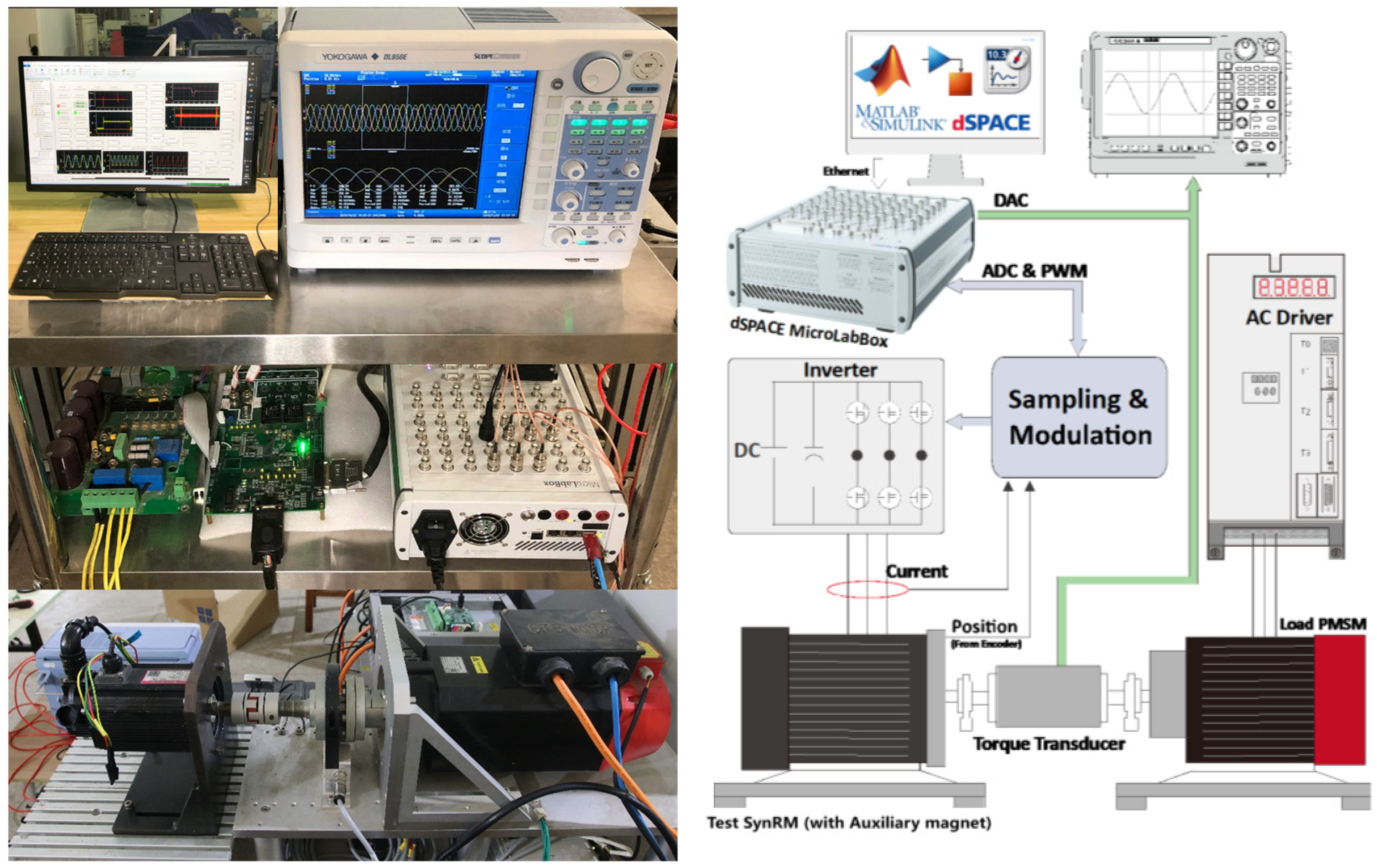
5. Experiment Results and Analysis

Figure 13 shows the experiment circumstance of the SynSM, a dSPACE MicroLabBox real-time platform is used to realize the control law of SynRM. The parameters of the SynRM are shown in

Table 2. The parameters of the SynRM.

The Parameters	The Value of the Parameters
Number of pole pairs	3
Stator resistance (Ω)	3.11
d-axis inductance (mH)	52.61
q-axis inductance (mH)	152.76
Permanent magnet flux linkage (Wb)	0.3064
Rotor inertia (kg·m2)	0.0042
Viscous damping (N·m·s)	0.002

. The switch frequency of PWM is set to 10 kHz. The injected voltage is set to 100 V and the frequency is set to 1000 Hz. The DC-link voltage is set to 500 V and the dead-time of inverter is set to 5 us. In experiments, the reference speeds are set as 200 rpm, 350 rpm, and 500 rpm, respectively. In order to highlight the influence of current harmonics, there is no external load, but the load motor connected to SynRM itself will be equivalent to a light load of about 1.4 N·m.

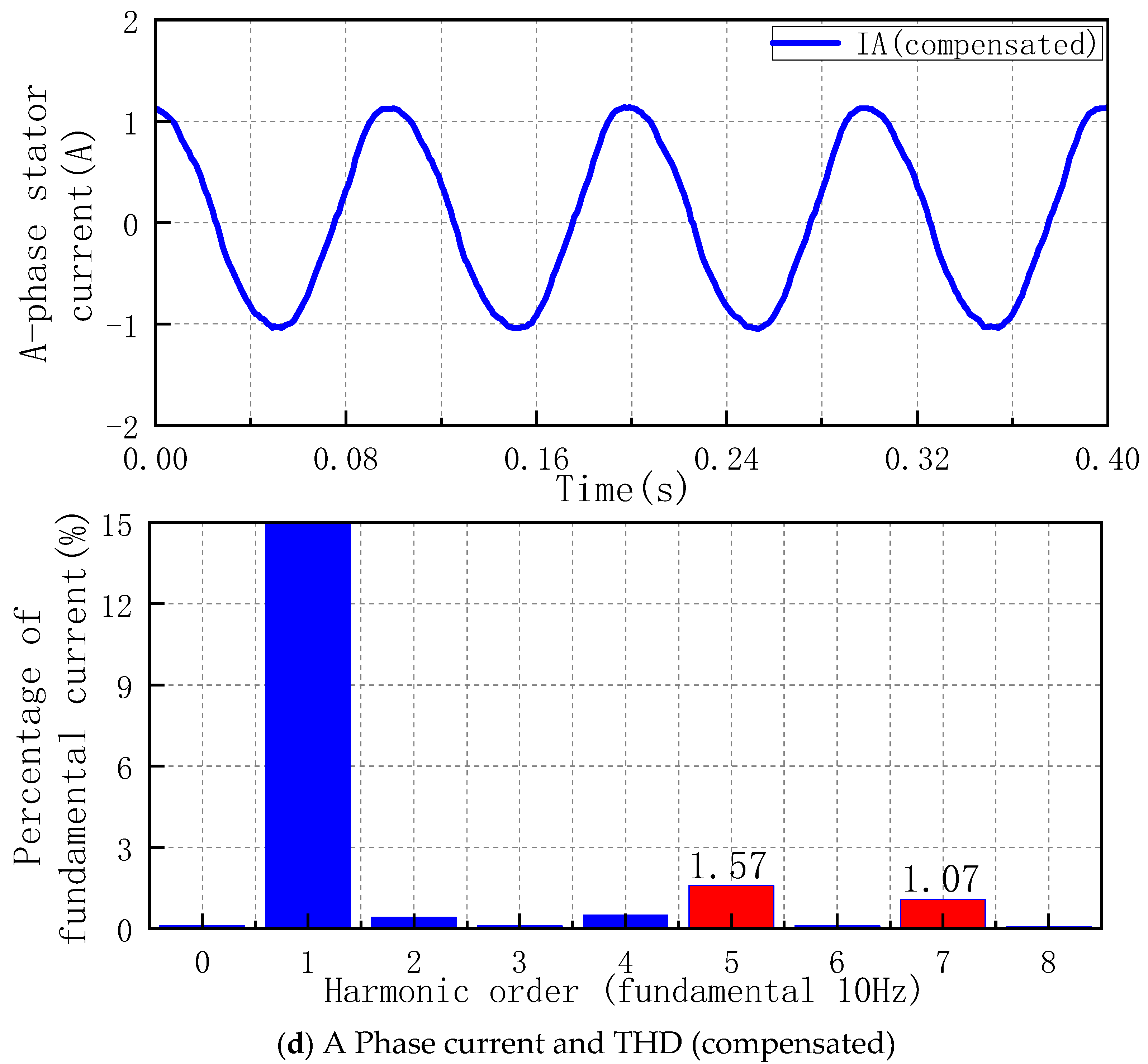
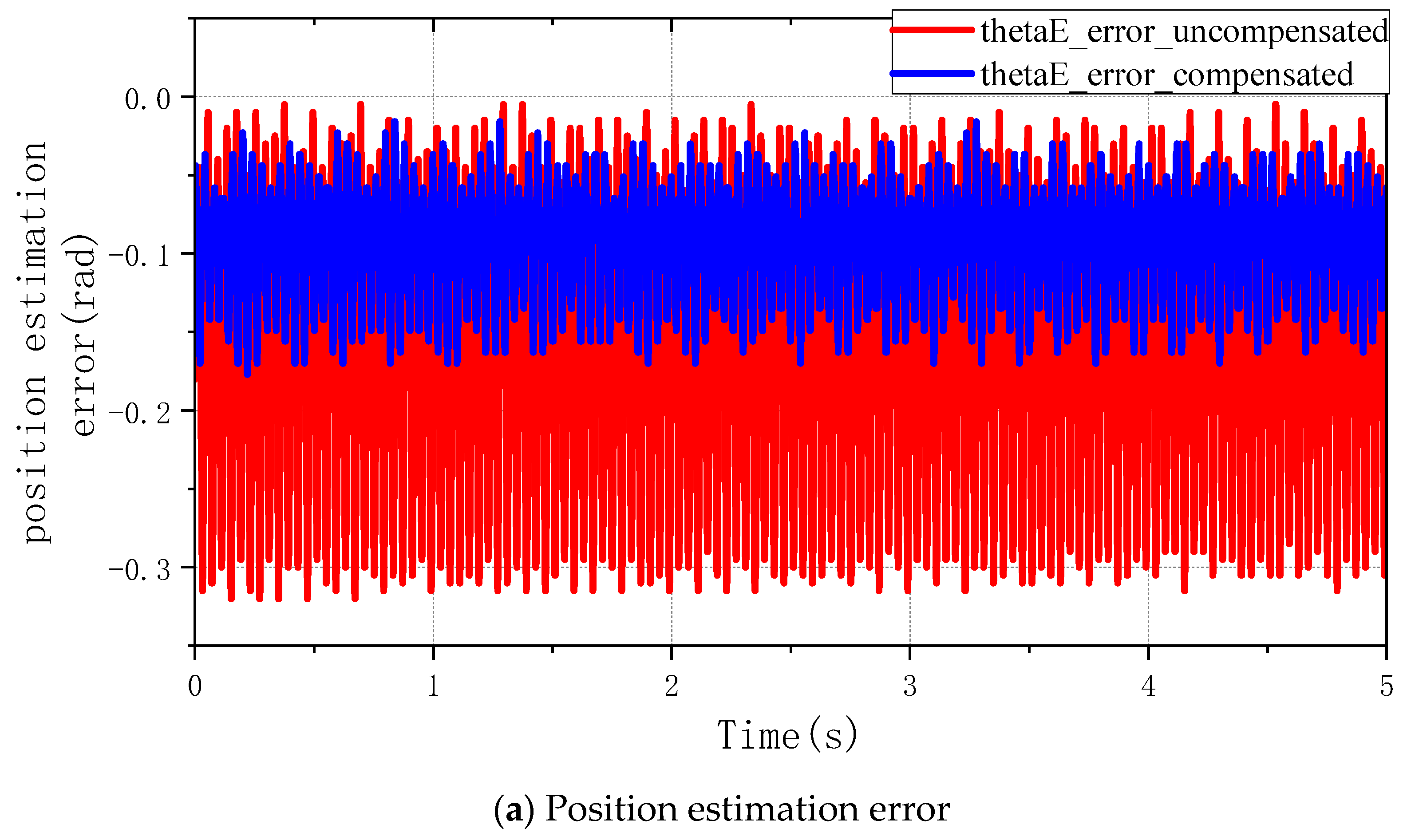
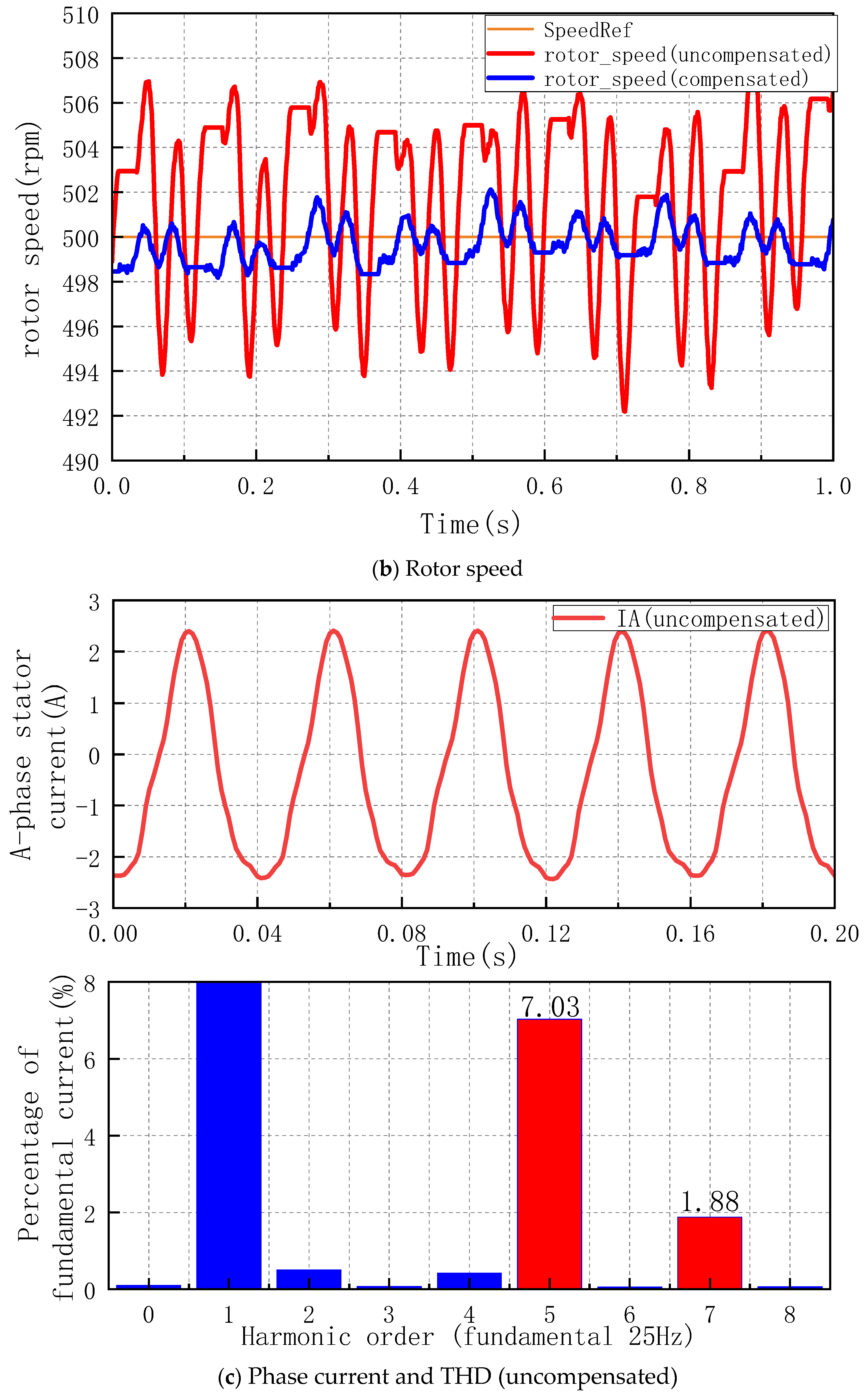
5.1. Uncompensated/Compensated Experiment and Result Analysis

In the first experiment, the speed command value is 200 rpm, the load motor is not powered on, and there is no additional load. Experiments are performed with and without dead-time effect compensation. Figure 14a shows the error between estimated electric angle ${\theta }_{ee}$ and real electric angle ${\theta }_{er}$ under these two conditions. Before using the compensation method proposed in this paper, the average and peak values of errors are −0.108 rad and −0.207 rad, respectively. With the filter-free dead-time compensation, the average value of error reduces to −0.048 rad, and the peak value reduces to −0.121 rad, which decreases by 55.5% and 41.5%, respectively. Meanwhile, the difference between the peak and mean electrical angle errors is reduced by 73.7%, which will significantly reduce the system torque fluctuation, as shown in Figure 14b. Figure 14c,d shows the A-phase stator current and their FFT results under compensated and uncompensated conditions. The non-fundamental components of the compensated A-phase current decreases significantly. Without compensation, the THD of A-phase current is 20.71%, of which the 5th and 7th harmonic components are 13.82% and 6.18%, respectively. With dead-time effect compensation, THD of A-phase current decreases to less than 3%, among which the 5th and 7th harmonic components are 1.57% and 1.07%, respectively, and the overall reduction is 86.8%. Comparing the experimental data of the two cases, the effect of the proposed methods is very obvious.

The experimental data are shown in Figure 15 when the speed instruction value is 350 rpm. Without compensation, the THD of A-phase current is 14.43%, the 5th and 7th harmonic contents are 11.21% and 3.14%, respectively. With the proposed methods, the THD of A-phase current decreased significantly to 2.64%, and 5th and 7th harmonics contents decreased to 1.06% and 1.41%, respectively. After compensation, the average and peak values of errors are −0.062 rad and −0.126 rad, which decreased by 55.07% and 52.10%, respectively. The difference between average and peak decreased from 0.121 rad to 0.064 rad, which is 47.10% lower than that without compensation. With the improvement of estimation accuracy, the data in Figure 15b show that the speed fluctuation of the SynRM before and after compensation decreases from −4.12~+4.37 rpm to −0.87~+1.14 rpm during the 1 s recording period. The steady-state performance of the SynRM system has been greatly improved.

When the third set of experiments with the speed instruction value of 500 rpm is carried out, the frequencies of the 5th and 7th harmonic current reach 125 Hz and 175 Hz, respectively. The frequency of the injected square-wave voltage cannot be considered to be much greater than the frequency of the harmonic current. Under this condition, the variation of harmonic current within sampling steps has a significant impact on the accuracy of high frequency signal separated without filters. As shown in Figure 16a, the average value of electrical angle error reaches −0.162 rad while the peak value is −0.311~0.318 rad when the motor is running steadily under this condition, which is already a large error. Due to the large position estimation error, the speed ripple of the rotor during the 1 s data recording period is ±8 rpm. After using the compensation method proposed in this paper, the A-phase current THD is reduced by 73.53%, and the sum of the 5th and 7th harmonic content is reduced from 7.91% to 2.11%. As the amplitude of harmonic current decreases, the average electrical angle error decreased from −0.162 rad to 0.087 rad, while the peak decreased from 0.318 rad to 0.167 rad. During the 1 s data recording period, the speed fluctuation under compensated state decreased by 81.3% to −1~+2 rpm compared with that under uncompensated condition. The experimental data show that the compensation method proposed in this paper achieves a good compensation effect without filter, and the steady-state performance of the system is better than that before the introduction of the compensation method.

5.2. Comparision and Analysis of Experimentation Data for Different Speed Conditions

As shown in Figure 14c, Figure 15c, and Figure 16c, under 200 rpm, 350 rpm, and 500 rpm conditions, the 5th and 7th harmonic components of the stator current decrease gradually, which are 20.0%, 14.35%, and 7.91%, respectively. This is due to the increase in the stator current caused by the higher rotor speed and the heavier equivalent load of the motor. Additionally, according to (21), the increase in the harmonic impedance also reduces the amplitude of the harmonic current. According to the deduction in (16), the position estimation error caused by the dead-time effect current increases with the higher angular velocity at medium and low speeds. As shown in Figure 14a, Figure 15a, and Figure 16a, with the increase in rotor speed, the peak values of electrical angle estimation error are −0.207 rad, −0.263 rad, and −0.318 rad for the three rated speeds. The larger the position estimation error, the faster the motor runs, and the greater the ripple of rotor speed. The increase in the error is slightly larger than the theoretical expectation, which may be due to the combined effect of other factors besides the dead-time effect and the harmonic current. For example, because the experimental motor is a permanent-magnet-assisted SynRM, the actual motor cannot meet the standard of an ideal motor in design. Affected by machining errors and tooth-groove effect, the magnetic field generated by ferrite installed on the rotor usually contains a large number of harmonics. Due to the cross-coupling phenomenon caused by the increase of current, the d-axis inductance changes, and the sensorless position solution is very dependent on the accuracy of parameters, etc.

In the three groups of experiments, the compensation method proposed in this paper has a good effect. According to the data of Figure 14d, the phase current THD has been reduced to less than 3%. The higher the speed of the experimental group, the lower the harmonic contents after compensation. After adopting the compensation method proposed in this paper, the larger the given speed of the experimental group, the greater the angle error and speed ripple when the rotor operates stably. This is because the higher the frequency of residual harmonic current, the more significant the influence according to Equations (16), (17), and (21). At the same time, it may also be affected by the harmonic generated by the ferrite permanent magnet and the performance degradation of the controller caused by the change of inductance parameters, but this paper will not discuss this in detail.

6. Conclusions

This paper presents a new error source sensorless rotor position estimation at low injection frequency and a dead-time compensation method suitable for filter-free HF square-wave voltage-based sensorless vector control systems. The sources of electric angle estimation errors caused by dead-zone harmonic currents are discussed in detail in this paper. The feasibility, the effect of reducing stator current THD, and the effect of reducing position estimation error of the new dead-time effect compensation method are fully proved by theoretical derivation and experimental results in this paper. Compared with previous studies, the new error sources proposed in this paper point out other error sources besides voltage distortion factors. The experimental results also show that the proposed filter-free dead-time compensation method still has good effect without filters and sensors. After reducing the harmonic current content, the accuracy of sensorless position estimation is significantly better than that of the state without compensation.

References

1. Tsujii, Y.; Morimoto, S.; Inoue, Y.; Sanada, M. Effect of Inductance Model on Sensorless Control Performance of SynRM with Magnetic Saturation. In Proceedings of the 2022 International Power Electronics Conference (IPEC-Himeji 2022-ECCE Asia), Himeji, Japan, 15–19 May 2022; pp. 2687–2693. [Google Scholar] [CrossRef]
2. Li, C.; Wang, G.; Zhang, G.; Xu, D. High Frequency Torque Ripple Suppression for High Frequency Signal Injection Based Sensorless Control of SynRMs. In Proceedings of the 2019 IEEE Applied Power Electronics Conference and Exposition (APEC), Anaheim, CA, USA, 17–21 March 2019; pp. 2544–2548. [Google Scholar] [CrossRef]
3. Li, C.; Wang, G.; Zhang, G.; Zhao, N.; Xu, D.G. Adaptive Pseudorandom High-Frequency Square-Wave Voltage Injection Based Sensorless Control for SynRM Drives. IEEE Trans. Power Electron. 2020, 36, 3200–3210. [Google Scholar] [CrossRef]
4. Alberti, L.; Bottesi, O.; Calligaro, S.; Kumar, P.; Petrella, R. Self-adaptive high-frequency injection based sensorless control for IPMSM and SynRM. In Proceedings of the 2017 IEEE International Symposium on Sensorless Control for Electrical Drives (SLED), Catania, Italy, 18–19 September 2017; pp. 97–102. [Google Scholar] [CrossRef]
5. Nikowitz, M.; Schrodl, M. Stability- and Sensitivity-Analysis of a Sensorless Controlled Synchronous Reluctance Machine using the Back-EMF Model. In Proceedings of the 2020 23rd International Conference on Electrical Machines and Systems (ICEMS), Hamamatsu, Japan, 24–27 November 2020; pp. 234–239. [Google Scholar] [CrossRef]
6. Scalcon, F.P.; Volpato, C.J.; Lazzari, T.; Gabbi, T.S.; Vieira, R.P.; Grundling, H.A. Sensorless Control of a SynRM Drive Based on a Luenberger Observer with an Extended EMF Model. In Proceedings of the IECON 2019 - 45th Annual Conference of the IEEE Industrial Electronics Society, Lisbon, Portugal, 14–17 October 2019; pp. 1333–1338. [Google Scholar] [CrossRef]
7. Martinez, M.; Laborda, D.F.; Reigosa, D.; Fernandez, D.; Guerrero, J.M.; Briz, F. SynRM Sensorless Torque Estimation Using High-Frequency Signal Injection. IEEE Trans. Ind. Appl. 2021, 57, 6083–6092. [Google Scholar] [CrossRef]
8. Setty, A.R.; Wekhande, S.; Chatterjee, K. Adaptive signal amplitude for high frequency signal injection based sensor less PMSM drives. In Proceedings of the 2013 IEEE International Symposium on Sensorless Control for Electrical Drives and Predictive Control of Electrical Drives and Power Electronics (SLED/PRECEDE), Munich, Germany, 17–19 October 2013; pp. 1–5. [Google Scholar] [CrossRef]
9. Liang, B.; Wang, Y.; Wei, J. A Compensation Method for Rotor Position Estimation of PMSM Based on Pulsating High Frequency Injection. In Proceedings of the 2020 23rd International Conference on Electrical Machines and Systems (ICEMS), Hamamatsu, Japan, 24–27 November 2020; pp. 2128–2132. [Google Scholar] [CrossRef]
10. Yoon, Y.-D.; Sul, S.-K. Sensorless control for induction machines using square-wave voltage injection. In Proceedings of the 2010 IEEE Energy Conversion Congress and Exposition, Atlanta, GA, USA, 12–16 September 2010; pp. 3147–3152. [Google Scholar] [CrossRef]
11. Li, W.; Liu, J. Improved High-Frequency Square-Wave Voltage Signal Injection Sensorless Strategy for Interior Permanent Magnet Synchronous Motors. In Proceedings of the IECON 2019—45th Annual Conference of the IEEE Industrial Electronics Society, Lisbon, Portugal, 14–17 October 2019; pp. 3205–3209. [Google Scholar] [CrossRef]
12. Wu, X.; Feng, Y.; Liu, X.; Huang, S.; Yuan, X.; Gao, J.; Zheng, J. Initial Rotor Position Detection for Sensorless Interior PMSM With Square-Wave Voltage Injection. IEEE Trans. Magn. 2017, 53, 8112104. [Google Scholar] [CrossRef]
13. Zhou, J.; Liu, J. An Improved High Frequency Square Wave Injection Permanent Magnet Synchronous Motor sensorless Control. In Proceedings of the 2021 6th International Conference on Control and Robotics Engineering (ICCRE), Beijing, China, 16–18 April 2021; pp. 101–105. [Google Scholar] [CrossRef]
14. Shi, W.-W.; Du, J.-W.; Jia-Wei, D. Sensorless control of Permanent Magnet Synchronous Motor based on rotating coordinate system considering dead-time. In Proceedings of the 2016 IEEE International Conference on Power and Renewable Energy (ICPRE), Shanghai, China, 21–23 October 2016; pp. 57–61. [Google Scholar] [CrossRef]
15. Hwang, C.-E.; Lee, Y.; Sul, S.-K. Analysis on the position estimation error in position-sensorless operation using pulsating square wave signal injection. In Proceedings of the 2017 IEEE Energy Conversion Congress and Exposition (ECCE), Cincinnati, OH, USA, 1–5 October 2017; pp. 844–850. [Google Scholar] [CrossRef]
16. Zhu, Z.Q.; Li, Y.; Howe, D.; Bingham, C.M. Compensation for Rotor Position Estimation Error due to Cross-Coupling Magnetic Saturation in Signal Injection Based Sensorless Control of PM Brushless AC Motors. In Proceedings of the 2007 IEEE International Electric Machines & Drives Conference, Antalya, Turkey, 3–5 May 2007; pp. 208–213. [Google Scholar] [CrossRef] [Green Version]
17. Hwang, C.-E.; Lee, Y.; Sul, S.-K. Analysis on Position Estimation Error in Position-Sensorless Operation of IPMSM Using Pulsating Square Wave Signal Injection. IEEE Trans. Ind. Appl. 2018, 55, 458–470. [Google Scholar] [CrossRef]
18. Yanying, W.; Peng, W.; Zhen, W. Sensorless Control of Permanent Magnet Synchronous Motor with Double Frequency Square Wave Voltage Injection. In Proceedings of the 2021 IEEE 4th International Electrical and Energy Conference (CIEEC), Wuhan, China, 28–30 May 2021; pp. 1–6. [Google Scholar] [CrossRef]
19. Kim, D.; Kwon, Y.-C.; Sul, S.-K.; Kim, J.-H.; Yu, R.-S. Suppression of Injection Voltage Disturbance for High-Frequency Square-Wave Injection Sensorless Drive with Regulation of Induced High-Frequency Current Ripple. IEEE Trans. Ind. Appl. 2015, 52, 302–312. [Google Scholar] [CrossRef]
20. Kim, K.-C.; Ahn, J.S.; Won, S.H.; Hong, J.-P.; Lee, J. A Study on the Optimal Design of SynRM for the High Torque and Power Factor. IEEE Trans. Magn. 2007, 43, 2543–2545. [Google Scholar] [CrossRef]
21. Zhang, G.; Wang, G.; Xu, D. Initial position detection method of permanent magnet synchronous motor based on unfiltered square wave signal injection. J. Electrotech. 2017, 32, 7. (In Chinese) [Google Scholar] [CrossRef]
22. Swathy, T.V.; Abhilash, T.V. High performance vector control of PMSM with dead-time compensation. In Proceedings of the 2012 IEEE International Conference on Power Electronics, Drives and Energy Systems (PEDES), Bengaluru, India, 16–19 December 2012; pp. 1–6. [Google Scholar] [CrossRef]
23. Xu, Z.; Yang, K.; Zheng, Y.; Yang, F.; Zhang, Y.; Song, P. Torque-Ripple reduction in Permanent Magnet Synchronous Motor Based on LADRC and Repetitive control. In Proceedings of the 2021 24th International Conference on Electrical Machines and Systems (ICEMS), Gyeongju, Republic of Korea, 31 October–3 November 2021; pp. 1777–1781. [Google Scholar] [CrossRef]
Figure 1. High-frequency signal and fundamental signal.
Energies 15 09539 g001
Figure 2. Sensorless rotor position estimation.
Energies 15 09539 g002
Figure 3. A three-phase PWM voltage-source inverter with SynRM load.
Energies 15 09539 g003
Figure 4. Six error voltage vectors differ by 120° from each other.
Energies 15 09539 g004
Figure 5. HF square-wave voltage, HF response current, and sampled fundamental current.
Energies 15 09539 g005
Figure 6. DC component, 6th and −6th harmonics of dq-axis current.
Energies 15 09539 g006
Figure 7. Ideal and actual separated dq-axis HF current.
Energies 15 09539 g007
Figure 8. Compensation voltage vectors for dead-time effect.
Energies 15 09539 g008
Figure 9. Space position of different current vectors.
Energies 15 09539 g009
Figure 10. Relationship between θ and compensation voltage vectors.
Energies 15 09539 g010
Figure 11. Forward and back lag angles for switching angle π/6.
Energies 15 09539 g011
Figure 12. Improved relationship between θ and compensation voltage vectors.
Energies 15 09539 g012
Figure 13. Experimental setup.
Energies 15 09539 g013
Figure 14. Experiment data for 200 rpm condition.
Energies 15 09539 g014aEnergies 15 09539 g014bEnergies 15 09539 g014c
Figure 15. Experiment data for 350 rpm condition.
Energies 15 09539 g015aEnergies 15 09539 g015b
Figure 16. Experiment data for 500 rpm condition.
Energies 15 09539 g016aEnergies 15 09539 g016bEnergies 15 09539 g016c