Abstract
The aim of this work is to adapt the methods of optical Hilbert diagnostics for the visualization and study of inverse diffusion H2/O2 flame. The diagnostic complex is implemented on the basis of the IAB-451 device with modified optical filtering. Visualization of phase perturbations induced by the studied medium in a probing multiwave light field is performed via polychromatic Hilbert and Foucault-Hilbert transformations in combination with registration and RGB-per-pixel processing of the dynamic structure of the images. From solution to the inverse problem of Hilbert optics using a physically justified initial approximation of the problem under consideration, the temperature field of the flame is reconstructed and the value of the H2, H2O, O2 and N2 concentrations may be restored.
1. Introduction
Diffusion flames can be classified into two types: normal diffusion flame (NDF), where the fuel flows into an oxidizing environment, and inverse diffusion flame (IDF), formed by an oxidizer jet surrounded by a fuel atmosphere. The IDF configuration provides cleaner combustion, improved flame stability, and wider concentration ranges of combustion [1]. The IDF is used in various chemical technologies, for example, in non-catalytic partial oxidation of methane [2]. The IDF characteristics differ from the NDF configuration. Differences that occur in the flame structure change qualitatively the mechanism of soot formation [3]. For hydrogen fuel of IDF, appearance of flame regions, where the combustion temperature exceeds the adiabatic combustion temperature of a homogeneous mixture of fuel and oxidizer, is noted in [4,5]. The parametric model [6] of a flame in the Burke-Schumann approximation gives fairly simple relationships that allow one to estimate the magnitude of the effect of superadiabatic combustion depending on the Lewis number of the chemical system and the intensity of convective transfer through the flame front. The estimates [6] agree satisfactorily with the results of measuring the combustion parameters of highly dilute mixtures of hydrogen with an inert gas in air [5]. The structure of the IDF is influenced not only by the ratio of fuel and oxidizer, but also by the aerodynamics of the reacting flow. Depending on αf (oxidizer excess ratio) and Re, several types of hydrogen-oxygen inverse flame are distinguished [7]. Simultaneous measurements of temperature and composition in a hydrogen-oxygen IDF can provide information about the internal structure of the reacting medium, which is important for predicting the properties of such flames. The development of optical information technologies causes a growing interest in their applications for flame diagnostics.
Modern optical diagnostic tools using the LIF and RAMAN spectroscopy methods allow obtaining data on the flame temperature and composition in a wide range of conditions [8]. At the same time, the approaches based on measuring the refractive index of a gaseous medium are relevant. In combination with the methods of optical flame tomography [9] such approaches have great potential. Two-dimensional flame temperature distribution is obtained in [10] from the refractive index distribution using the Gladstone-Dale equation. A method that combines emission and moiré tomography was proposed in [11]. Background schlieren imaging in combination with computed tomography was successfully used in [12] to reconstruct the field of instantaneous 3D refractive indices of a turbulent flame.
In order to measure simultaneously the temperature and composition, two-wave methods were developed [13]. These methods, as it is noted in [14] are very sensitive to errors in determining the coefficient gas mixture refraction n, since it is a weak function of the wavelength. It is possible to increase the accuracy of measurements by additionally applying other optical methods, for example, using spectrometries composition diagnostics [14]. A method for simultaneous measurement of n and temperature in the reacting flow, which also allows obtaining more accurate results, is proposed in [15]. A method for estimating the temperature distribution in an asymmetric flame using high-contrast stereoscopic photography is described in [16]. Spectral reconstruction of the temperature fields using color ratio pyrometry and interferometric tomography is reported in [17]. The optical diagnostics based on the methods of Hilbert optics in combination with pixel-by-pixel processing of the dynamic structure of the visualized phase structures induced by the temperature fields is an example adapted to the problems of flame research [18].
Diagnostics of the temperature of a hydrocarbon fuel flame preliminarily mixed with air using interferometry methods makes it possible to obtain data on the temperature field with good accuracy in the approximation of the independence of the refractive index of the gas mixture from the composition. The same approaches works with a diffusion flame. However, in the case of a hydrogen flame, the assumption of a weak dependence of the refractive index on the gas mixture composition may turn out to be insufficient.
In this paper, the method of polychromatic of Hilbert optics is proposed to study the structure of the flame. Just as in [14], the refractive index of a gas mixture n is a weak function of wavelength. The application of the Tikhonov regularization method to solve weakly defined systems of equations makes it possible to increase the accuracy of temperature determination and obtain simultaneous fields of temperature and composition in the flame.
2. Experimental Setup
The diagnostic complex is implemented on the basis of the IAB-451 optical shadow device with modified nodes for generating the probing field and Hilbert filtering (Figure 1a). When organizing combustion of a hydrogen-nitrogen mixture, a burner, combining two coaxially arranged stainless steel tubes, was used (Figure 1b). The gas flow rate and composition of the H2/N2 fuel mixture were determined using the El-Flow Bronkhorst flow meter and precision digital generator of gas mixtures UFPGS-2 (10, 11, and 12).
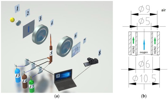
Figure 1.
Experimental research setup. (a) optical scheme; (b) geometry of the burner device.
The setup includes an illumination module consisting of a light source 1 (an RGB LED with operating wavelengths λ1 = 636 nm, λ2 = 537 nm and λ3 = 466 nm), a collimator lens 2, and a slit aperture 3 placed in the front Fourier plane of the objective 4, forming a probing field. The properties of the radiation source were refined using the “Kolibri-2” spectrometer [19]. The Fourier spectrum of phase disturbances induced in the probing field by the flame 5 is localized in the frequency plane of the lens 6, where the quadrant Hilbert filter 7 is placed, whose orientation is consistent with the diaphragm 3. The lens of the digital video camera 8 performs the inverse Fourier transform of the Hilbert spectrum field of optical phase density of the flame. Depending on the spectral characteristics of the light source, analytical or Hilbert-conjugate optical signals are formed on the photomatrix. The fields of optical phase density fixed by the camera are processed by a computer 9, which also controls the partial composition of the mixture of gases coming from cylinders 13–15 into the burner 5.
The Hilbert transform has the properties of redistributing the energy of an optical signal from a region of low spatial frequency to a high-frequency region. The extremes and gradients of the phase optical density of the medium under study are transformed into Hilbert-visualized structures fixed by a photomatrix. The spatial distribution of Hilbert structures provides information about perturbations of the optical density of the phase caused by the temperature field. In the experiment, a random sample of RGB-hilbertograms of the oxygen jet in the associated fuel stream “H2(65%) + N2(35%)” was visualized and recorded, exiting into the atmosphere and recorded at random times.
2.1. Theoretical Justification
The refractive index of the burning mixture is determined according to the Gladstone-Dale formula [20,21]:
where p is the pressure; pn.c. is the atmospheric pressure under normal conditions (measured value of atmospheric pressure in the room); T is the temperature; Tn.c is the temperature under normal conditions (in the room); Ak and Bk are the dispersion coefficients of the kth component of the burning mixture; λ is the wavelength of the radiation source; Ck is relative molar concentration of the kth component of the reacting mixture. In the flow under consideration, we can take p = pn.c with good accuracy.
In the approximation of the axial symmetry of the torch, the phase density of the probing light field in the studied section of radius R can be expressed as follows:
where r2 = x2 + z2; k = 2π/λ, is the wavenumber of the probing field; n(r,y) is the refractive index at distance r from the flame axis and n∞ is the refractive index of air. The probing light beam propagates along axis z and the flame cross-section is described in x, z coordinates. The choice of cross-section position is given by coordinate y.
The air refractive index n∞ is determined as
where T∞ is the room temperature; and are the dispersion coefficients of the kth component of dry air; Aw and Bw are the dispersion coefficients of water; is the molar fraction of the kth component of dry air and Cw is the molar fraction of water vapors in air.
The experiment was carried out under the following conditions: atmospheric pressure in the room p∞ = 99,400 Pa; temperature T∞ = 298 K; relative air humidity of 29%.
2.2. RGB-Hilbertogram Processing
The solution to the inverse problem—reconstruction of T and Ck in the cross-section—requires restoration of the value of the phase function Δψ from each hilbertogram recorded in the RGB channels and determination of refractive index , solving the Abel equation. The method of finding Δψ in each RGB channel of a hilbertogram is described in [18].
As a result, to find the refractive indices of the gas mixture of the flame, a system of linear algebraic equations was compiled using (1):
Equation (4) can be written as the operator equation:
where J is the linear operator; q is the sought solution and f is the given function.
where .
The approximation of diffusion combustion often assumes that the flame front is impermeable to the fuel and to the oxidizer. This allows the flow to be split into an oxidizer zone and a fuel zone. In the hydrogen-oxygen diffusion flame at a temperature in the reaction zone of ~3000 K, this approach ceases to work. Water formed during combustion at high temperatures becomes a source of a noticeable amount of hydrogen. This means that the number of optical “channels” must increase by the corresponding number of times. It should be noted that the matrix of system (5) belongs to the class of poorly defined ones , since the dependence of the refractive index on is weak. An increase in the number of equations does not allow one to obtain reliable estimates of the flame composition and temperature from the solution to the system of Equation (4).
The task of determining the temperature and concentrations of the medium components by refractive indices for different wavelengths:
Due to the small difference in wavelengths in the RGB range, it is incorrect. Therefore, its regularization is carried out—the problem of minimizing the functional is considered
using a stabilizer of the 0-th order, where the function is determined based on additional information.
Thus, with the help of an auxiliary non-negative functional, the deviations of values from the known right-hand side of are stabilized. The solution of the Equation (10) is found by the formula:
When choosing the regularization parameter α close to 0, the problem will be close to the original one and, therefore, incorrect. If the parameter α is close to 1, the problem will be correct, but the solutions will be far from true and closer to . Thus, the task is to determine the function —the parameter of the stabilizing functional and find the optimal value α. To do this, the following algorithm is proposed. In the first step, a regularized solution is found according to Formula (11) when = 0 is selected, and the parameter α is selected so that all concentrations of the components are positive.
The next step is to determine the refractive indices at three wavelengths from the calculated values of concentrations and temperature, and the procedure for calculating the equilibrium composition of the medium is performed, which allows us to obtain a new estimate of the initial approximation = 0. This procedure is organized as follows: In the case of diffusion combustion at any point in space (n − 1) = f(T, Ci), the refractive index is a function of temperature and composition, which in turn have an unambiguous relationship between each other T = T(Ci).
When constructing the initial approximation of the regularization ≠ 0, we use the conditions of chemical equilibrium. For some dimensionless temperature profile:
Let us write down the heat release function per unit mass per unit time, where Hu is the calorific value of the fuel and αf is oxidizer-to-fuel equivalence ratio:
for αf > 1 (lean fuel mixture), L0—is the stoichiometric coefficient and for αf < 1 (rich mixture).
On the other hand, the heat release function can be defined as:
where —average process heat capacity at constant pressure (weight fractions of components and ).
For simplicity, we assume that the heat capacities of the fuel and oxidizer do not depend on temperature (CPf = Const and CPox = Const)). Then, the new distribution of the oxidizer-to-fuel equivalence ratio will be:
for a lean and rich mixture, respectively.
The ratio of heat capacities can be replaced by the ratio of specific enthalpy:
which will speed up the process of convergence of the solution. The temperature for the new distribution αf(x) is found by the Gladstone-Dale (1) formula.
For the obtained distributions of the oxidant excess coefficient and temperature, we calculate the equilibrium composition. The work used the freely available program “Terra”, developed by OIVT RAS MOSCOW [16]. Next, applying the Gladston-Dale equation, we obtain a new temperature distribution corresponding to the reduced composition. The procedure can be repeated the required number of times.
The technique was tested on the distribution by the coefficient of excess oxidizer:
where, , x0 and xF—the position of the fuel boundary and the flame front, respectively.
After five repetitions, the difference in concentrations did not exceed 2% of the “true” initial value. For a given distribution n(x), convergence to the same solution is obtained when the initial conditions change.
This procedure was applied to the distribution (n − 1) = f(x) obtained in the experiment. The bill went in two directions: from the axis of the oxygen jet through the fuel and from the air into the fuel. The initial distribution of the composition was taken by step functions. For the calculation of “oxygen + fuel” it is αf = Const >> 1 at x < 2.5 mm (no fuel) and αf = 0 at x > 2.5 mm (no oxidizer); for the calculation of “air + fuel”: αf = 0 at x < 4.5 mm and αf = Const >> 1 at x < 4.5 mm at xmin =2.5 mm. The solutions on the right and left were stitched together. Based on the obtained distributions of temperature and “frozen composition”, the spatial distribution of the equilibrium composition with a given number of components is calculated, which was then used as an initial approximation for Tikhonov regularization.
Using this data, the values of the function for the next step are determined. At the final step, according to Formula (3), a regularized solution , is found. The regularization parameter α is determined in such a way that the standard deviation of the extremes of the calculated , hilbertograms and the extremes of the experimental hilbertograms for all three wavelengths is minimal.
Let us apply this procedure to the distribution , obtained in the experiment for the oxygen jet in the co-current flow of fuel “H2(65%) + N2(35%)” escaping into the atmosphere (Figure 2). The green line marks the section in which the temperature distribution is measured. The colored segment marks the position of the edge of the outlet section of the tube. We will count in two directions from the oxygen jet axis through the fuel and from the air into the fuel. Let us also take the step functions as the initial compositional distribution. For the calculation of “oxygen + fuel” it will be: αf = Const >> 1 for x < 2.5 mm (no fuel) and αf = 0 for x > 2.5 mm (no oxidizer); for “air + fuel” calculation: αf = 0 at x < 4.5 mm and αf = Const >> 1 at x < 4.5 mm at xmin = 2.5 mm. The initial temperatures will also be different. In the first case, this is recovered according to the Gladstone-Dale equation for oxygen on axis (); in the second case, this is recovery by air in free space (). As it was shown earlier, repeating the recovery procedure five times is sufficient to converge to the steady state solution with good accuracy. The solutions on the right and left are stitched together. Based on the obtained distributions of temperature and “frozen composition”, the spatial distribution of the equilibrium composition with a given number of components is calculated, and it is used as the second stabilizing function q02 for the Tikhonov regularization Equation (10).
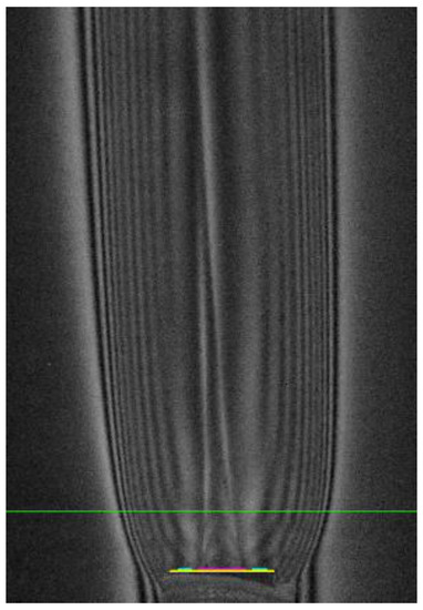
Figure 2.
Hilbertogram of the co-current fuel flow H2(65%) + N2(35%) escaping into the O2 flow: G-channel—λ2 = 537 nm, mentioned cross-section y = 6 mm.
Radial temperature distributions in cross-section y = 6 mm, obtained in each RGB channel of the hilbertogram without taking into account the influence of the refractive indices of fuel combustion products (by air) are shown in Figure 3a. The difference between these diagrams demonstrates how strong the influence of combustion products is in the resulting phase function of the probing light field. The distribution of temperature obtained by calculating q02 is compared in Figure 3b with the temperature obtained as a result of the second iteration of the Tikhonov regularization. Note that the diagrams of the equilibrium temperature and the temperature obtained using regularization are fairly close. It is important to note that taking into account the dependence of the refractive index on the composition makes it possible to obtain superadiabatic temperature values.
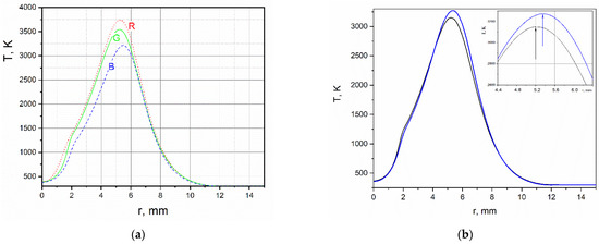
Figure 3.
(a) Radial distribution of temperature obtained in the air approximation in each RGB-channel of the hilbertogram; (b) black curve—equilibrium distribution of temperature; blue curve—temperature obtained by the Tikhonov regularization.
Figure 4 shows the obtained temperature and composition distributions in the section y = 6 mm from the section of the burner device. Dark rectangles mark the position of the walls of the coaxial tubes of the burner device relative to the axis of symmetry of the flow at r = 0. The figure field shows a PLIF visualization of the radical OH (Proc. of the XXXVIII STS, 2022, in Russ.). In the considered flow mode, the fuel hydrogen at a height of y = 6 mm fully reacted. As it can be seen at high temperatures of the diffusion flame ~3000 K, water decomposes in the vicinity of the front and, therefore, the hydrogen content reaches 7%.
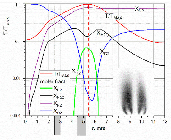
Figure 4.
Reconstructed temperature and composition values in H2/O2 flame.
3. Analysis of Results
To assess the reliability of the data obtained, an inverse problem was solved, which consists of reconstructing phase functions and Hilbertograms from temperature fields and mole fractions of fuel combustion products in each RGB channel and comparing the results with those obtained in the experiment. The reliability criterion is the coincidence of the local extrema of the Hilbert bands of the experimental and reconstructed Hilbertograms.
In the R-channel, the average shift of the reconstructed Hilbert bands with respect to the experimental ones was
where is the number of the Hilbert strip. By analogy in G and B channels: ≈ 0.17 mm, ≈ 0.16 mm. As an example, Figure 5 shows the experimental and reconstructed in the B-channel Hilbertograms of the flame cross section y = 6 mm.
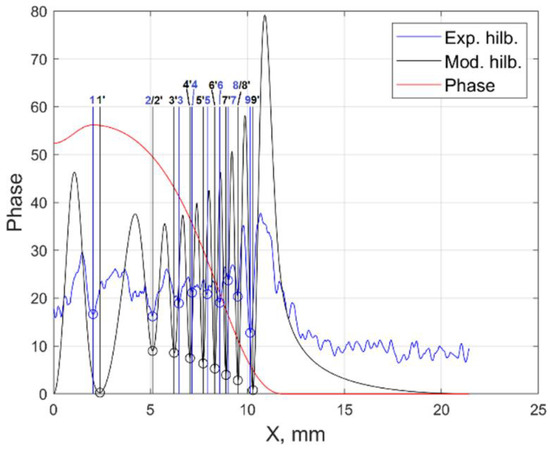
Figure 5.
The experimental and reconstructed in the B-channel Hilbertograms of the flame cross section y = 6 mm.
From a comparison of the experimental and reconstructed Hilbert bands, an estimate was made of the error in determining the refractive index during registration in each of the RGB channels. The refractive index is a function of temperature and mole fractions of fuel combustion products For fixed , the estimate of the temperature error was obtained from the analysis of the investigated section of the Hilbert image of the plume (Figure 6). At the point x = 11.4 mm of this section, the temperature spread was: the maximum value is ±35 K, the minimum is ±1.5 K.
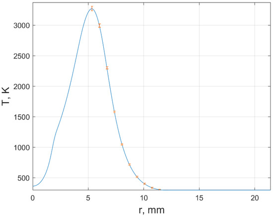
Figure 6.
The estimates of the temperature error in of the flame cross section y = 6 mm.
4. Conclusions
The inverse problem of reconstruction of the temperature fields and mole fractions of the fuel combustion products is solved by the Hilbert polychromatic diagnostic method on the example of the inverse diffusion flame of H2(65%) + N2(35%) fuel mixture in O2. The dynamic phase structure of the flame is visualized. The obtained data show that the method enables verification of the measurement results via comparison of experimentally recorded hilbertograms and those calculated from the obtained values of temperature and composition of the medium under study. One of important advantages of the proposed method for flame diagnostics is the potential for simultaneous temperature and composition measurements with a spatial resolution of up to several microns, which makes it possible to study the entire range of scales of the reacting flow up to Kolmogorov scale.
Author Contributions
Conceptualization, V.L.; Methodology, E.A., Y.D. and A.T.; Investigation, V.A., E.A. and O.Z.; Writing—original draft, O.Z. and A.T.; Writing—review & editing, E.A., Y.D. and V.L.; Funding acquisition, V.L. All authors have read and agreed to the published version of the manuscript.
Funding
This research was funded by Ministry of Science and Higher Education of the Russian Federation, grant number 075-15-2020-806.
Conflicts of Interest
The authors declare no conflict of interest.
References
- Zheng, S.; Qi, C.; Zhou, H. Experimental Investigations of Temperature Distribution in Non-Premixed Flames with Different Gas Compositions by Large Lateral Shearing Interferometry. J. Quant. Spectrosc. Radiat. Transf. 2019, 224, 445–452. [Google Scholar] [CrossRef]
- Song, X.; Wu, R.; Zhou, Y.; Wang, J.; Wei, J.; Li, J.; Yu, G. Understanding the Influence of Burner Structure on the Stability and Chemiluminescence of Inverse Diffusion Flame. Int. J. Hydrogen Energy 2021, 46, 24461–24471. [Google Scholar] [CrossRef]
- Demarco, R.; Jerez, A.; Liu, F.; Chen, L.; Fuentes, A. Modeling Soot Formation in Laminar Coflow Ethylene Inverse Diffusion Flames. Combust Flame 2021, 232, 111513. [Google Scholar] [CrossRef]
- Takagi, T.; Xu, Z.; Komiyama, M. Preferential Diffusion Effects on the Temperature in Usual and Inverse Diffusion Flames. Combust Flame 1996, 106, 252–260. [Google Scholar] [CrossRef]
- Kochergin, D.O.; Abdrakhmanov, R.H.; Lukashov, V.V.; Terekhov, V.V. On the Structure of Direct and Inverse Diffusion of the Hydrogen-Air Flame. Sci. Bull. Novosib. State Tech. Univ. 2016, 62, 195–204. [Google Scholar] [CrossRef][Green Version]
- Law, C.K.; Chung, S.H. Steady State Diffusion Flame Structure with Lewis Number Variations. Combust. Sci. Technol. 1982, 29, 129–145. [Google Scholar] [CrossRef]
- Utria, K.; Labor, S.; Kühni, M.; Escudié, D.; Galizzi, C. Experimental Study of H2/O2 Downward Multi-Fuel-Jet Inverse Diffusion Flames. Exp. Therm. Fluid Sci. 2022, 134, 110583. [Google Scholar] [CrossRef]
- Cheng, T.S.; Chen, J.-Y.; Pitz, R.W. Raman/LIPF Data of Temperature and Species Concentrations in Swirling Hydrogen Jet Diffusion Flames: Conditional Analysis and Comparison to Laminar Flamelets. Combust Flame 2017, 186, 311–324. [Google Scholar] [CrossRef]
- Yan, Y.; Qiu, T.; Lu, G.; Hossain, M.M.; Gilabert, G.; LIU, S. Recent Advances in Flame Tomography. Chin. J. Chem. Eng. 2012, 20, 389–399. [Google Scholar] [CrossRef][Green Version]
- Najafian Ashrafi, Z.; Ashjaee, M. Temperature Field Measurement of an Array of Laminar Premixed Slot Flame Jets Using Mach-Zehnder Interferometry. Opt. Lasers Eng. 2015, 68, 194–202. [Google Scholar] [CrossRef]
- Guo, Z.; Song, Y.; Yuan, Q.; Wulan, T.; Chen, L. Simultaneous Reconstruction of 3D Refractive Index, Temperature, and Intensity Distribution of Combustion Flame by Double Computed Tomography Technologies Based on Spatial Phase-Shifting Method. Opt. Commun. 2017, 393, 123–130. [Google Scholar] [CrossRef]
- Grauer, S.J.; Unterberger, A.; Rittler, A.; Daun, K.J.; Kempf, A.M.; Mohri, K. Instantaneous 3D Flame Imaging by Background-Oriented Schlieren Tomography. Combust Flame 2018, 196, 284–299. [Google Scholar] [CrossRef]
- El-Wakil, M.M.; Jaeck, C.L. A Two-Wavelength Interferometer for the Study of Heat and Mass Transfer. J. Heat Transf. 1964, 86, 464–466. [Google Scholar] [CrossRef]
- Konishi, T.; Ito, A.; Kudo, Y.; Narumi, A.; Saito, K.; Baker, J.; Struk, P.M. Simultaneous Measurement of Temperature and Chemicalspecies Concentrations with a Holographic Interferometer and Infrared Absorption. Appl. Opt. 2006, 45, 5725. [Google Scholar] [CrossRef] [PubMed]
- Zhang, H.; Cong, B.; Zhang, F.; Qi, Y.; Hu, T. Simultaneous Measurement of Refractive Index and Temperature by Mach–Zehnder Cascaded with FBG Sensor Based on Multi-Core Microfiber. Opt. Commun. 2021, 493, 126985. [Google Scholar] [CrossRef]
- Huang, Q.; Wang, F.; Yan, J.; Chi, Y. Simultaneous Estimation of the 3-D Soot Temperature and Volume Fraction Distributions in Asymmetric Flames Using High-Speed Stereoscopic Images. Appl. Opt. 2012, 51, 2968–2978. [Google Scholar] [CrossRef] [PubMed]
- Dreyer, J.A.H.; Slavchov, R.I.; Rees, E.J.; Akroyd, J.; Salamanca, M.; Mosbach, S.; Kraft, M. Improved Methodology for Performing the Inverse Abel Transform of Flame Images for Color Ratio Pyrometry. Appl. Opt. 2019, 58, 2662–2670. [Google Scholar] [CrossRef] [PubMed]
- Arbuzov, V.; Arbuzov, E.; Dubnishchev, Y.; Zolotukhina, O.; Lukashov, V. Method of Polychromatic Hilbert Diagnostics of Phase and Temperature Perturbations of Axisymmetric Flames. In Proceedings of the 31st International Conference GraphiCon 2021, Nizhny Novgorod, Russia, 27–30 September 2021; Volume 31, pp. 369–378. [Google Scholar]
- Zarubin, I.A.; Labusov, V.A.; Babin, S.A. Characteristics of Small-Sized Spectrometers with Different Types of Diffraction Gratings. Ind. Lab. Diagn. Mater. 2019, 85, 117–121. [Google Scholar] [CrossRef]
- Ioffe, B.V. Refractometrician Methods in Chemistry; Chemistry: St. Petersburg, Russia, 1983. [Google Scholar]
- Karaminejad, S.; Askari, M.H.; Ashjaee, M. Temperature Field Investigation of Hydrogen/Air and Syngas/Air Axisymmetric Laminar Flames Using Mach–Zehnder Interferometry. Appl. Opt. 2018, 57, 5057–5067. [Google Scholar] [CrossRef] [PubMed]


Publisher’s Note: MDPI stays neutral with regard to jurisdictional claims in published maps and institutional affiliations. |
© 2022 by the authors. Licensee MDPI, Basel, Switzerland. This article is an open access article distributed under the terms and conditions of the Creative Commons Attribution (CC BY) license (https://creativecommons.org/licenses/by/4.0/).