Abstract
The increasingly widespread use of electric vehicles requires proper planning of the charging infrastructure. In addition to the correct identification of the optimal positions, this concerns the accurate sizing of the charging station with respect to energy needs and the management of power flows. In particular, if we consider the presence of a renewable energy source and a storage system, we can identify strategies to maximize the use of renewable energy, minimizing the purchase costs from the grid. This study uses real charging data for some public stations, which include “normal” chargers (3 kW and 7 kW) and “quick” ones (43 kW and 55 kW), for the optimal sizing of a photovoltaic system with stationary storage. Battery degradation due to use is included in the evaluation of the overall running costs of the station. In this study, two different cost models for battery degradation and their influence on energy flow management are compared, along with their impact on battery life.
1. Introduction
The transition from fossil fuel-powered transport to electric mobility is considered a necessary step to tackle greenhouse gas emissions. However, the widespread use of electric vehicles may cause some concern, mainly related to the impact of battery charging and the need to carefully plan the charging infrastructure. The development of the charging infrastructure has an impact on the electricity grid, particularly on the ability to respond to requests for power. One way to limit these impacts is to integrate the charging structure with stationary storage systems and photovoltaic sources (PV), in order to contain power peaks on the grid, through on-site energy production. The factors influencing the choice of sizes and possible implementation are many, including the space available, the additional cost, the extent of the reduction in the withdrawal from the network, the diversity of the storage, and PV sizes.
Several studies have approached the problem of planning and operation schedules of charging infrastructures. There are several issues to consider in the correct design of charging infrastructures for electric road vehicles. For a public charging infrastructure, parameters such as the number of users, the number of charging points and the influx time distribution influence the quality of the service, as investigated in [1]. The complex relationship between charging services and electricity network requires careful planning and operation of the charging infrastructure, which takes into account traffic congestion, loads on the electricity grid and charging costs [2]. An approach for optimizing the siting and sizing of charging stations considering the interactions between the energy and transport industries is presented in [3]. The work takes into account the load capacity constraints to evaluate the feasibility of the implementation, also taking into account the economic convenience. In [4], electric physical constraints are included in a mathematical profit maximization model, which is designed to distribute appropriate capacities at the charging stations. The charging infrastructure could be integrated with smart grids, as well as with different types of renewable energy sources and stationary electric storage systems [5].
The use of renewable energy in power recharging would lead to an increase in acceptance by potential users of EVs [6]. In this context, Energy Storage Systems (ESS) can be used to balance the generation of electricity from renewable energy sources. This solution is particularly interesting for fast charging stations [7] or in stand-alone solutions [8]. In [9], an energy management scheme is introduced which provides uninterrupted daytime charging at a constant price, for a Charging Infrastructure (CI) equipped with a photovoltaic (PV) system and Battery Energy Storage System (BESS). In addition, Vehicle-to-Grid (V2G) technology is incorporated into the charging system to improve the payback schedule of the existing PV grid system. For a similar configuration of the charging station, an intelligent optimization and control algorithm is proposed in [10], which aims to reduce operating costs. The algorithm foresees: the optimization of the energy management programs of the day before; the determination of the charge price based on participation in the V2G; the optimization of energy management programs of the hour before; and real-time control. In [11], an optimal management of power flows in real time for a CI-PV-BEES system is presented, formulated as integer mixed linear programming, for an intelligent infrastructure based on microgrids for charging Electric Vehicles (EV), with the aim of minimizing the total cost of energy in different weather conditions. Particular attention is also paid to a rapid charge of electric vehicles and related issues [12]. In [13], the authors consider a charging station for electric vehicles, with PV and BESS installed. The approach involves examining first the problem of the operation of the charging station for electric vehicles and then the optimal planning of the stations. The load is synthetized using a stochastic model based on an M/M/c/K birth–death Markov model. In [14], the configuration optimization process aims to maximize the expected profit of the station considering the investment and operational costs, maintenance, and penalties linked to customer dissatisfaction due to waiting times or lack of service. The determination of the optimal size and charging station management was performed for various application environments. The EV flow was simulated using M/G/N/K queues.
Despite the large body of studies, there appears to be a lack of studies based on real data to improve the sizing and control strategies of charging stations [15]. In the present work, the study is based on data on real charges recorded for one year at eleven public stations installed in the metropolitan area of Barcelona. Although the optimization of CI-PV-BESS operation has been extensively studied, the influence of stationary battery duration has not been fully explored. In [16], a proposal was made to take battery duration into account in optimizing the power flow in a CI-PV-BESS system with V2G. The optimization problem is faced using a multilayer procedure, according to a set of priorities aiming at maximizing the use of photovoltaics and minimizing the amount of energy purchased from the grid. The procedure involves a stochastic approach to addressing uncertainty in the load and production of renewable energy. However, it only enters into the determination of the BESS operating energy cost by means of a function dependent on the State of Charge (SOC), while the impact of the reduction in battery capacity over time on the functionality of the infrastructure was not taken into account. In [17], the aging of the lead–acid batteries that compose the storage was taken into account to avoid overloads and overdischarges in a stand-alone configuration for the battery charger, although no issues related to the profitability of the investment were investigated. In [18], a hypothetical network of fast charging stations on highways is considered for a simulated charging request. The charging station consists of three 120 kW chargers and a BESS of two possible sizes: 250 and 650 kW. The comparison between the investments for these two BEES sizes is made with the net present value. The aging of the BESS is taken into account, considering the current, the operating temperature and the time of use, using models calibrated on cells for specific types of batteries for electric cars. However, the parameters of the aging models are specific to chemistry and battery type. Unlike the approaches proposed so far in the literature, this paper focuses on the degradation costs for the BESS and their influence on the CI power fluxes and impact on investment costs. In particular, we compare a linear cost function, in which the degradation cost is simply proportional to the energy exchanged, with one dependent on SOC. Subsequently, we explicitly include battery aging in the system operations to correctly evaluate the time horizon of the investment. The aim of the authors is to show that different, albeit simple, degradation models can influence the determination of the optimal energy fluxes, which in turn has consequences for battery usage and thus for battery life. A graphical representation of the proposed approach is reported in Figure 1. Furthermore, the proposed analysis and results are based on real data derived from public CI in the metropolitan area of Barcelona (AMB). As far as the authors know, this is the first time that the impact of different battery aging models can have on the operation of the charging station and on the actual investment time horizon has been studied. In Section 2, we present an approach for the optimal sizing of a Renewable Energy Source (RES) and BESS for a CI an urban area. In Section 3, we evaluate the power flow at the station on typical days and highlight the influence of different battery models on power exchanges. Section 4 presents the conclusions.
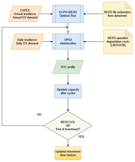
Figure 1.
Flowchart of the proposed approach.
2. Charging Infrastructure Sizing
In the present section, we determine the optimal size of a RES with a BESS system for a CI in an urban area. In particular, the considered RES is a photovoltaic (PV) system, since it is the most suitable for an urban environment. The analysis uses real data on charging events at public CI in AMB. The PV system consists of a finite number of identical solar panels, with inverters and Balance-of-System (BoS). The BESS consists of a finite number of identical battery units of common technology integrated with a BoS. In our model, we will disregard BoS in the analysis, as it usually does not affect too much the project costs [19]. The influences of soft costs on the charging station construction can also have a big impact on the deployment of the infrastructure, both on the final costs and the installation time [20]. However, these costs can greatly vary from one country to another, and in time, making an exact estimation difficult. For this reason, soft costs are not included in the following cost analysis.
2.1. BESS and PV Cost
In this study, we are interested in Behind-The-Meter (BTM) applications for BESS, i.e.: commercial and residential use, for which capacity ranges from 0.01 to 0.25 MWh [21]. Usually, the battery technologies used for BTM applications are Li-ion and lead–acid. To compare different technologies, the Levelized Cost of Storage (LCOS) metric was introduced by Belderbos, et al. [22], which is analogous to levelized cost of energy for energy sources. This index takes into account many parameters, such as Capital Expenditure (CAPEX), Operational Expense (OPEX), life duration, and discount rate. In Table 1, we summarize LCOS for Li-ion and lead–acid batteries for BTM applications, according to different sources. Although the reported costs show some discrepancies, the LCOS for Li-ion and lead–acid batteries are overall comparable. A study of the International Renewable Energy Agency (IRENA) [23] reports that the CAPEX will decrease for all technologies by the year 2030, estimating a drop of about 60% for Li-ion system capital costs, and of 50% for lead–acid systems. Instead, OPEX is assumed to remain unchanged, as the maintenance costs are already very low compared to CAPEX. With this consideration, we will focus on Li-ion technology for the BESS. The CAPEX is calculated as an average of the 2018 and 2025 costs (0.35 EUR/Wh) [24]. We did not consider OPEX costs, since they are negligible compared to the CAPEX costs. We did, however, consider degradation costs, as illustrated in the next session. As for the PV system, the European Technology and Innovation Platform for Photovoltaics estimates that the cost for a 50 MWp utility system is about 65% of the residential one; for a 1 MWp system, it is 80% and for a 50 kWp (commercial) system, it is 90% of the residential cost [25]. Since the cost in 2014 of a turnkey photovoltaic utility scale was 955 EUR/kWp with a reduction to 823 and 724 in 2020 and 2025, respectively [26], we can deduce that the PV price in 2020 for residential is around 1.2 EUR/Wp, while for commercial, it is around 1.0 EUR/Wp. We did not include any analysis of COVID-19 influence on PV system price. Thereafter, CAPEX for the PV system is estimated at 1.2 EUR/Wp.

Table 1.
LCOS for different battery systems.
2.2. Charging Events Dataset and Analysis
The optimization problem has been applied to the case study of Barcelona, which is a demo city in the H2020 UserChi Project [31]. The dataset used in the present work contains the registration of the charging events AMB in 2019 [32]. It consists of two files, the first including charging events information such as: Charging Point Identification (CP id), Charging Point (CP) name, type of connector, charging start time and stop time, duration, energy consumption, vehicle, and model. The last two fields are optional. The other file contains static information about the charging points, such as address, longitude, latitude, and type of connectors at the CP, CP makers. Each CP id corresponds to one of the following configurations:
- (a)
- Two Schuko 3 kW 16A mode 1 sockets;
- (b)
- One Mennekes 43 kW 63 A mode 3, one CHAdeMO 55 kW 125 A mode 4, one COMBO CCS 55 kW 125 A mode 4;
- (c)
- Two Schuko 3 kW 16 A mode 1 and two Mennekes 7 kW 16 A mode 3.
In ten CP locations, the two configurations (a) and (b) are present, so we can refer to this combination as a charging infrastructure (CI). The configuration (c) is present only in one location, so it will be considered in the statistical analysis, but not included in the CI analysis and size determination. In the following, the term “normal” chargers includes 3 kW and 7 kW, while “quick” refers to 43 kW and 55 kW. The statistical analysis of the data can be found in [33]. After the filtering procedure, we obtained a data set with 36,194 records. Table 2 reports some figures on the usage of the CPs, while the relevant statistical parameters for the charges (mean value and standard deviation of charge duration and energy delivered) are reported in Table 3. As an input to the procedure of system sizing, for each month of the year, a synthetic daily load profile representative of all load profiles in the month was created. From the database, we extract the number of charges, the energy required, and the duration of the charges as a function of the hour of the day, for each month. For quick charges, we excluded charges that delivered less than 1 kWh and/or with power less than 1 kW. For normal charge, we excluded those with less than 0.1 kWh delivered. We reconstruct the time distribution of the number of users at the stations, according to the arrival time and taking into account the duration (expressed in hours, which represents the time scan unit) and the energy delivered during the charges, to obtain the a posteriori frequency distribution for the arrivals at the CIs and the average power required. Using this distribution, we can construct a “most-probable” load profile for each month and a given number of users per day. To emphasize the role of PV and BESS, we selected the most crowded station: 14 users per day for quick charges and 2 for normal ones. The average energy of the charge profile obtained is set equal to the average energy of the entire set. Some examples of load profiles are reported in Figure 2.
Table 2.
Usage rate of charging points for different typologies.
Table 3.
Statistical parameters for charges.
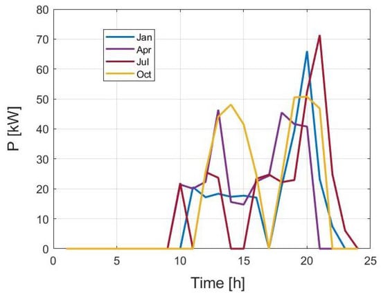
Figure 2.
Examples of synthetic load profiles for Barcelona for some months of the year.
The procedure illustrated above is one of the possible options for creating a synthetic profile, and different approaches can lead to different results for the optimal dimension of the system [33].
2.3. Size Optimization Procedure
A diagram for the proposed system is shown in Figure 3. A DC bus connects the different energy sources with the CI, while the inverters guarantee the voltage stability. The BESS stores the energy from the PV system, and/or from the grid when the electricity cost is low. The energy stored in the BESS is then used to charge electric vehicles when the PV source is absent and/or the cost of energy from the grid is high. Based on technical-economic constraints, an algorithm determines the optimal configuration of the system according to the operating conditions and plant costs [33], and the following input data:
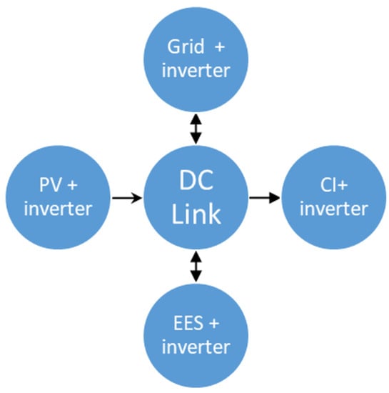
Figure 3.
Proposed system for charging infrastructure with a renewable energy source.
- The market price of electricity;
- Productivity and cost of the photovoltaic system;
- Costs of the storage system;
- Charging profiles.
Through the economic criterion of the Net Present Value (NPV) [34,35] by projecting the analysis over the entire depreciation period of the infrastructure, it is possible to determine the optimal system solution and identify the basic information for the preliminary design of the CI. An investment is advantageous when the NPV is positive, i.e., when the project incomes are sufficient to repay the initial outlay by providing a net gain. The NPV is assessed over a time horizon (N in years) and is a function of the cash flows relating to the investment made and the interest rate considered (k); it can be expressed as follows:
where:
N: time horizon of the investment in years, fixed in 15 years;
: cash flows in the t-th year, calculated as the difference among cash flow without and with the PV + BESS system;
I: initial investment, calculated as the sum of the PV and BESS CAPEX;
k: interest rate, fixed in 3%.
In the monthly analysis, a representative day of the average monthly production of photovoltaics and the average monthly cost of electricity purchased from the grid is considered. The 15-year NPV is used as a basis for comparison of the different investment projects, which is a trade-off between the duration of a PV system (20–30 years) and a CI and BESS (10–15 years).
The power flows coming from the sources through the conversion systems are summed up in the common DC bus. In particular, it is possible to write the balance of the input powers coming to the DC bus:
where:
: power withdrawn from the grid;
: power supplied by the photovoltaic system;
: discharge power of the battery pack;
: charging power of the battery pack;
: power required by the load;
: efficiency of the network converter;
: efficiency of the photovoltaic system converter;
: efficiency of the bidirectional converter of the battery pack, discharge mode;
: efficiency of the bidirectional converter of the battery pack, charge mode;
: efficiency of the output converter.
The optimization problem aims at minimizing the objective function represented by the daily operating cost of the charging infrastructure () consisting of two components: the cost of the energy supplied by the grid and the cost of the degradation of the storage system. In particular, the optimization problem was expressed as follows:
where:
: is the price of the energy at time h [EUR/kWh];
: the power withdrawn from the grid at time h [W];
: the sample time, in the present 1 h;
: the degradation cost for the EES [EUR/h].
The system model must respect a series of constraints, listed below:
Equations (4)–(7) define the operating limits of the system based on the minimum and maximum power of the sources. and , Equation (8), are binary variables necessary to prevent the battery pack from being simultaneously charged and discharged. Equation (9) limits the power that can be drawn from the photovoltaic system to the maximum extractable power in the h-th hour. The constraint (10) links the state of charge at the hour () to that one of the previous hour () as a function of the charge/discharge power used, the nominal energy stored by the battery pack and the charge and discharge efficiency of the storage system. According to the constraint (11), the must be within a minimum () and a maximum () to limit the depth of discharge and, therefore, the cost of degradation. The stability of the state of charge between one day and another is imposed by Equation (12). The following inputs have been used in the optimal size procedure:
- Price of electricity: the data for 2019 were downloaded from the Comision Nacional de los Mercados y la Competencia (CNMC) [36];
- Productivity of the PV system: data were taken from the “Performance of grid-connected PV” tool of the Photovoltaic Geographical Information System (PVGIS) [37]. The data contain the monthly production for installed peak PV power of 1 kWp and system loss of 14% (mounting configuration: tilt 35°, azimuth 0°) from the PVGIS-SARAH data base for the selected locations;
- Efficiencies of the conversion systems: efficiency values of 0.9 were used for all systems, except BESS, for which the value was set to 0.8;
- Required charging power profiles, as illustrated in the charging events dataset and analysis.
The battery size depends on many characteristics: in particular, the power is one key parameter in the size determination. However, battery performance is generally expressed in terms of different parameters, such as the maximum charge and discharge currents (that usually vary with temperature and aging), maximum, minimum, and operating voltage, and capacity. Since voltage V is not a linear function of SOC, power is also not a linear function of SOC, which makes it difficult to implement a simple algorithm for size optimization. This problem is partially overcome by the fact that the curve V vs. SOC for Li-ion batteries can be approximated by a straight line within the SOC range of 10–90%.
2.4. System Degradation
The degradation rate of the photovoltaic system is set at an average value of 0.5% per year of loss of productivity [38].
The battery duration is taken into account in two ways: for the calendar life, the duration is fixed to 15 years, while for life cycle it is assumed that the battery can last for fixed to = 10,000 charges and discharges cycles at 70% of Depth of Discharge (DOD), which leads to a full cycles at 70% DOD. This assumption considers current storage solutions performance, with up to 20 years and 5000 cycles at 100% DOD [39,40,41].
To model the degradation cost in the optimization procedure, we use a very simple model based on cycles counting (similar to the rain-flow counting). This choice allows the optimization model to be mixed linear integral, while a more realistic model would make it non-linear. However, in the size determination phase, this simple model is sufficient to consider the costs that derive from the battery usage.
Taking as cost per watt-hour of the battery degradation the price for the battery pack: = 0.35 EUR/Wh [24], we can obtain the cost for a full cycle with DOD = 70% as: .
The degradation cost for a generic cycle “i” is given by: .
2.5. Growth in Demand
In the analysis, we will also consider the projections in the growth of the electric car market. The share of electric vehicles is growing fast. According to the European Automobile Manufacturers’ Association (ACEA), the market share of electric cars in 2019 was 3.0%, which is one percentage point more than in 2018 [42]. According to forecasts by the International Energy Agency, electric cars, which accounted for 2.6% of global car sales and about 1% of global car stock in 2019, registered a 40% year-on-year increase. As a result of the continuous increase in sales, EVs are expected to account for about 7% of the global vehicle fleet by 2030 [43]. We will include a growing rate in the range 0–10% in the analysis.
2.6. Results
In the following, the results of the optimization problem for AMB case study are presented. The optimization problem was solved in MatLab using the “solve” command, which is an equations and system solver, in a linear programming problem defined by an optimization problem. Even though Equation (3) with constraints (4)–(12) represent a mixed-integer linear programming problem, it can be reduced to a linear programming problem, since the constraint (8) is implicitly satisfied when minimizing battery degradation costs.
Costs for the installation of CI are not considered as, for AMB, the local administrations promote the installation of CI in the streets. In this case, the municipalities act as a Charge Point Operator (CPO). Moreover, we consider the possibility of introducing subsidies programs oriented to the installation of PV panels for CI, similar to those already existing for residential PV systems [44].
As a first step, a PV system without BESS is considered. Without incentives for investment costs, the renewable source is not convenient. However, applying a 20% incentive on the PV investment cost, the NPV becomes positive and the optimal size for the PV system is around 23 kWp for the ideal case of converters’ efficiency equal to 1. In the more realistic scenario of efficiencies lower than 1, the optimal size is around 25.3 kWp. If the degradation of the PV system is included, the optimal size grows to 27.25 kWp. In the following, only a non-ideal system will be considered, unless explicitly stated.
If we allow increasing the demand with time, we obtain an increase of the PV size, as well as an increase in the corresponding NPV. In Figure 4, we show the results for different constant yearly growth rates. The NPV increases when the growth rate is higher than a threshold, around 5%. Correspondingly, the growth of PV size over this threshold slows down.
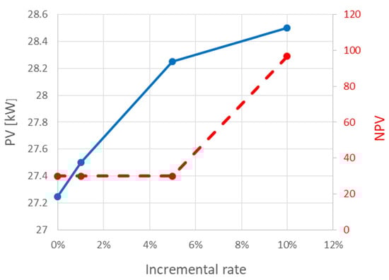
Figure 4.
Optimal PV sizing with no BESS (principal axis) and corresponding NPV (secondary axis) as a function of demand growth rate.
The increment of the NPV can be correlated to the increase in the self-consumption of the PV energy when the load demand increases.
To evaluate the size of the system components when a BESS is present, we initially consider a zero CAPEX for the BEES plant. We obtain that the investment is feasible if the incentives on PV costs are preserved: the optimal value for the PV increases to 39.5 kW with a BEES as large as 98 kWh. This BEES size guarantees that all the energy produced by the PV is entirely consumed by the CI. However, when the investment cost for the BESS is considered, there is no convenience in designing it to obtain the total self-consumption of the PV energy. In particular, if the BESS CAPEX is equal or greater than 0.35 EUR/kWh, the incentives of 20% should be extended to the total system investment cost to obtain a positive NPV. If a load demand increase is included, the optimal BESS size increases along with the PV size. If the load increases with a 5%, 1%, and 0% growth rate per year, and the BESS CAPEX is equal to 0.35 EUR/kWh, the optimal size for the PV in the is around 37 kW, 35 kW, and 33.5 kW, respectively. The relative values for the BEES are: 12.5 kWh, 13 kWh, and 13.5 kWh. The BESS optimal size increases as the load increases. This trend holds for all the scenarios investigated, independently from the values of CAPEX BESS and the incentives put in place. It is interesting noting that the ratio between the optimal BESS and PV sizes is constant with respect to the incremental rate, at a given BESS CAPEX. The dependence of the ratio from the CAPEX is reported in Figure 5. We can conclude that for the Barcelona scenario, the use of BEES with PV can lead to positive NPV values, if some incentive policies are put in place, and increase the self-consumption of renewable energy.
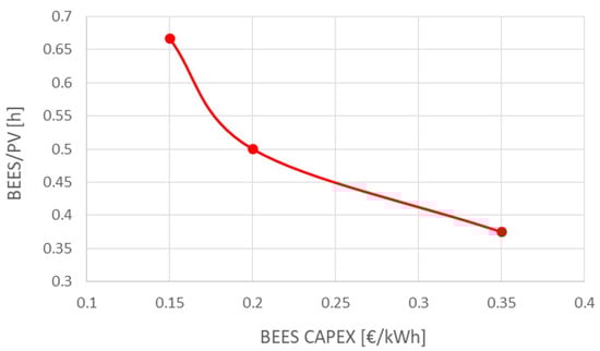
Figure 5.
BEES to PV ratio as a function of the BEES CAPEX.
3. Charging Infrastructure Operations
When the PV system is coupled with a BEES, there is the need for a control strategy to optimize the resources usage. In the present approach, the aim is to minimize the operating cost, which includes the purchase of energy from the grid and the degradation of the battery due to cycling, using Equation (2). Moreover, the BESS can participate to power-shifting from the grid, i.e., charge the BESS when the energy price of the grid is low and discharge it when the price is high. To solve the optimization problem for the CI operation, we use a linear programming solver that optimizes the use of the BESS according to the minimization of the costs, Equation (3), and maximization of the PV usage. To determine the optimal functioning of the CI, we used a probabilistic approach. In fact, some of the system inputs, such as PV production and the power required by vehicles in charging processes, are intrinsically random. The approach adopted is numerical and is based on the Monte Carlo (MC) method: for the charge method, the input data are obtained in a pseudo-random way starting from the Non-Parametric Distribution Function (NPDF) of the arrivals at the CI, and using the mean value and the variance of the duration of the charges and the energy required for each time interval. The workflow of the procedure is illustrated in Figure 6. Given the duration and average number of daily arrival, for each MC run, we construct a load profile from the a posteriori distribution of arrivals, assuming a Gaussian distribution for the charge duration and energy. In a similar way, from the monthly irradiation, we extract a most-probable profile and add Gaussian noise. These randomized synthetic charging and irradiation profiles are used in the algorithm to obtain the corresponding optimal BESS SOC distributions that minimize the operational costs. The ensemble of SOC distributions and power flows are then used in the statistical analysis to identify the statistically most favorable usage of the BESS to determine the optimal activity schedule for the following day.
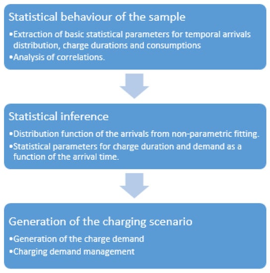
Figure 6.
Workflow of the scenarios creation procedure.
Influence of Battery Modeling
The goal of day-to-day management is to minimize operating costs—the sum of the cost of energy purchased from the grid—and the cost of battery degradation due to cycling. The quantification of BEES degradation costs during the operations influences the outcome of the procedure. In the following, we compare the results for different BEES degradation models. In particular, we analyze a linear cost model (LM), where the energy price is constant in all the SOC range: this means that the degradation is assumed to be unrelated to the depth of charge/discharge. The cost was determined as follows:
where is the price for battery cell, and is the life cycle expressed in number of full cycle. We allow the SOC to vary between 20% and 90%, to minimize battery degradation.
Applying Equation (3) to each run of the MC procedure, and averaging over the output, we can determine the most probable trend for the power fluxes in a given day. As an example, we illustrate the energy fluxes for two different months. For both sets of runs, we use the set PV size equal to 33.5 kW, with a BESS of 12.5 kWh. The energy price for the battery cell is = 0.15 EUR/Wh, which is an average price for 2019, although price is decreasing rapidly [45]. The results for the power distribution among the sources are reported in Figure 7. The top stacked histogram chart represents the contribution of the different energy sources to the power demand of the load (black line). In particular, the red bar is the grid contribution, the blue bar is the PV contribution, and the cyan is the BEES contribution. The yellow bar represents the PV power exceeding the load demand that can be sold to the grid, while the magenta is the power withdrawn from the grid or from the exceeding PV energy, to charge the battery. The blue line is the PV production. The green line represents the grid energy price. The bottom chart represents the SOC of the battery during the day. With the chosen parameters, the battery takes part in the power flux exchange helping the self-consumption. In fact, the surplus of PV power (the part of the blue bar exceeding the black line) is used to charge the battery, as it can be seen during the day of January (Figure 7a). From Figure 7b, it can be seen that a part of the PV energy produced in July is not absorbed by the BEES (yellow bar) since the battery SOC has already reached its maximum value. Although the details of the system behavior depend on the approaches used to model the battery degradation, it can be concluded that, for the operation of a CI with PV, the presence of the BESS is beneficial, since it decreases the energy withdrawn from the grid by increasing the exploitation of the PV production.
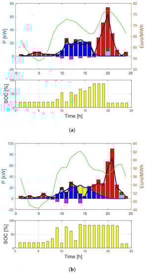
Figure 7.
Power fluxes and optimal SOC distribution for LM, of a CI with a 33.5 kW PV system and a 12.5 kWh BEES for AMB: (a) January, (b) July.
We compare the results thus obtained with the ones for a cost model where the battery energy price depends on the state of charge, as in [33]. We will refer to this model as the State of Charge Cost Model (SOCM). As in the LM, we made the hypothesis that charge and discharge have the same energy cost. In particular, we adopt the following cost function:
where C is a coefficient that is chosen so that the cost of a full cycle (0–100% SOC) is the same for LM and SOCM:
and is a constant introduced to avoid divergences. Its value influences the cost function shape. We use here the value 1, so that the SOCM function is as in Figure 8. We apply the MC procedure using either the LM or the SOCM model, over the same sets of random load and insulation profiles, and compare the average results over the runs. First of all, we calculate the CI OPEX for a typical day when BESS degradation cost is not considered, = 0. The results for four different months are reported in Table 4, along with the partition of PV and grid energy utilized to satisfy the load demand, and the number of complete cycles of the BESS in a day, obtained with the rain flow counting method. As it can be seen, the CI daily operating costs are reduced when a PV + BESS system is present, although the saving is different for each month. The percentage of PV energy used directly to satisfy the load demand or to charge the BESS depends more on the temporal distribution of the load rather than the seasonal production. Since we considered converters’ efficiencies smaller than one, the sum of the PV and grid contribution is greater than 1. In general, the BESS usage is more intense during summer and spring with respect to winter and autumn. The different models used for the battery degradation cost influence directly the average daily CI OPEX. A sensibility analysis is conducted for different life cycle span: 1250, 2500, and 5000 full cycles, both for LM and SOCM. We stress here that when aging is not explicitly included in the model, the life span enters only in the OPEX cost (13) and (14). We analyzed the yearly average values of the following variables: CI OPEX, partition of PV energy used, partition of grid energy used, and number of complete BESS cycles. If we limit the BESS depth of discharge to 20% and the upper SOC to 90% in the SOCM, the energy price is always lower than in LM (see Figure 8). We then relax any constraints for the SOC available range when using SOCM, since the highest price for high and low SOC values should limit the usage in these regions. As an example, Figure 9 reports the optimal SOC distribution for SOCM with = 5000 for a typical day of January (a) and July (b). Comparing with the SOC distribution obtained for LM with SOC boundaries, Figure 7, we see that for SOCM, the range used in a typical day is extended well below the 20% lower limit, although the upper SOC limit is very close to 90%. The influence on the CI OPEX of BESS life cycle is illustrated in Table 5, which reports some results obtained for LM and SOCM, for different life cycle durations. It is evident from the results in Table 5 that SOCM is not as sensitive to battery life duration as LM. Furthermore, the application of the SOCM model results in the lowest daily costs. By observing the energy flows, we can verify that the largest share of energy purchased from the grid belongs to the LM model when the battery life is 1250 cycles, and the smallest to SOCM, when the battery life is 5000 cycles. Indeed, the application of the SOCM model leads to an average CI OPEX lower than that obtained by LM with a null BESS OPEX and SOC in the range 20–90%, and equal to that of LM with a null BESS OPEX and no limitation on SOC, although with a slightly different partition of energy among the sources.
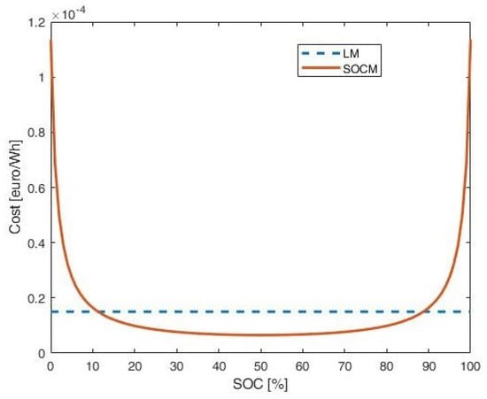
Figure 8.
Cost function for LM (dashed blue line) and SOCM (solid red line).
Table 4.
CI OPEX and source power partition when BESS OPEX is null.
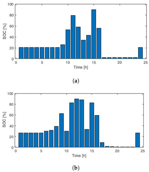
Figure 9.
Optimal SOC distribution for SOCM model of a CI with 33.5 kW PV and 12.5 kWh BEES for: (a) January, (b) July.
Table 5.
Average yearly figures for LM OPEX with different BESS life cycles, and for SOCM OPEX.
This shows that using SOCM the battery is exploited for greater depths of discharge, allowing to use a larger fraction of the energy produced by the PV, compared to the LM case, when SOC is limited to 20–90%. Furthermore, since the battery works mostly in the range around SOC = 50%, where on average the SOCM price is lower than LM (see Figure 7), even removing the SOC limitation, the CI OPEX continues to be lower when using SOCM than LM. The different use of the BESS in the two model influences the duration of the BESS itself. We thus explicitly include the capacity degradation in the models in order to evaluate the impact of the different usages on the BESS life duration. Let us consider a simple degradation model, in which the capacity decreases in proportion to the number of equivalent complete cycles performed. This model does not take into account the influence of depth of discharge or intensity of current on battery degradation. However, since a very broad time horizon is being analyzed, even a simplified model like this one can give some indications on the life expectancy of the BESS. If the declared BESS cycle life stated that after full equivalent cycles, the capacity has decreased by a x%, such that the final capacity is , where is the initial (nominal) capacity and x is the capacity reduction, the proposed aging model can be mathematically represented as follows:
where is the capacity at step k and is the number of full equivalent cycles at step k. Using the model (16), the trend of the relative capacity over the 15 years of the investment period is as reported in Figure 10, with = 40%.
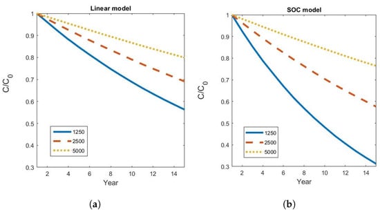
Figure 10.
Capacity degradation as a function of years, for different battery life durations and for (a) LM and (b) SOCM. Solid blue line: 1250 cycles; red dashed line: 2500 cycles; yellow dotted line: 5000. The trend is polynomial of degree 2 in all the cases.
As expected, the capacity diminishes at a higher rate when the expected life cycle is shorter. The SOCM leads to a faster degradation since it exploits a larger SOC range than LM. As an example, for a 1250 life cycle, the BESS reaches 60% of the initial capacity after 7 years with SOCM, while it takes 13 years with LM; for 2500 life cycle, the limit is reached after 14 years using SOCM, while it is not reached in the investment horizon of 15 years using LM. This means that the profit obtained in the OPEX CI with SOCM could be canceled by the need to purchase a second BESS, due to the achievement of the end-of-life condition of the first one.
4. Conclusions
In the present work, we consider the optimal dimensioning of a charging station equipped with a renewable energy source, and a storage system, based on the real charging requests of some public stations in the metropolitan area of Barcelona. Next, the procedure analyzes daily operations, identifying the power flows that maximize the use of renewable energy and minimize operating costs, including battery degradation. We analyzed the influence of different BESS degradation models that are used as OPEX functions. We use some simple approaches for battery modeling that could, however, be suitable in the evaluation of CI investment over a time horizon. We use some simple approaches for battery modeling that could, however, be suitable in the evaluation of CI investment over a time horizon. The main contributions of the paper are:
- To highlight the influence that different battery aging models can have on the operations and functioning of a charging station;
- To demonstrate that different BESS usage policies affect the investment time horizon. In this sense, a careful analysis of BESS performance is recommended during the design phase, in order to correctly calibrate the range of use and maximize the return on investment.
When we consider a degradation price model that depends on the SOC (SOCM), we obtain lower values for the operating CI costs than using a constant cost (LM). The SOCM is implemented without range restriction for BESS since the increment of the degradation costs toward low and high SOC values prevents the system usage in those regions. On the other hand, LM explicitly includes SOC limitation in the range [20–90%]. The results show that using SOCM lead to a greater number of cycles per day, and allows exploiting better the PV production with respect to LM. However, this translates into a higher number of full equivalent cycles per year, which brings to a shorter BESS life. This result directly influences the time horizon of the investment and should be considered in the economic evaluation of the investment. Furthermore, it could influence the operating policies at the CI by tuning the relative importance of the different components with respect to the CI operating costs. A more detailed and complex aging model can be included to take into account specific battery characteristics.
Author Contributions
Conceptualization, N.A. and M.D.M.; methodology, N.A., M.D.M. and G.T.; software, N.A. and M.D.M.; validation, N.A. and M.D.M.; formal analysis, N.A.; investigation, N.A., M.D.M. and G.T.; resources, N.A.; data curation, N.A.; writing-original draft preparation, N.A.; writing-review and editing, M.D.M. and G.T.; visualization, N.A. and M.D.M.; supervision, G.T.; project administration, N.A.; funding acquisition, N.A. All authors have read and agreed to the published version of the manuscript.
Funding
This work has been supported in part by the European Union’s Horizon 2020 research and innovation programme under grant agreement No. 875187. The results reflect only the authors’ view and the Agency is not responsible for any use that may be made of the information it contains.
Data Availability Statement
Data on charging events are available in Zenodo. https://doi.org/10.5281/zenodo.5721233, accessed on 4 November 2022.
Conflicts of Interest
The authors declare no conflict of interest.
Nomenclature
| Efficiency of the bidirectional converter of the battery pack, charge mode | |
| Efficiency of the bidirectional converter of the battery pack, discharge mode | |
| Efficiency of the network converter | |
| Efficiency of the output converter | |
| Efficiency of the photovoltaic system converter | |
| AMB | Metropolitan Area of Barcelona |
| BESS | Battery Energy Storage System |
| BoS | Balance of System |
| BTM | Behind the Meter |
| Price of the energy | |
| Degradation cost for the BEES | |
| CAPEX | Capital Expenditure |
| CI | Charging Infrastructure |
| CP | Charging Point |
| DOD | Depth of Discharge |
| ESS | Energy Storage System |
| EV | Electric Vehicle |
| LCOS | Levelized Cost of Storage |
| LM | Linear Cost Model |
| MC | Monte Carlo |
| NPDF | Non-Parametric Distribution Function |
| NPV | Net Present Value |
| OPEX | Operational Expenditure |
| Charging power of the battery pack | |
| Discharge power of the battery pack | |
| Power withdrawn from the grid | |
| Power required by the load | |
| PPV | Power supplied by the photovoltaic system |
| PV | Photovoltaic System |
| RES | Renewable Energy Source |
| SOCM | SOC Dependent Cost Model |
| SOC | State of Charge |
| V2G | Vehicle to Grid |
References
- Gunther, M.; Fallahnejad, M. Strategic Planning of Public Charging Infrastructure. In IUBH Discussion Papers—IT & Engineering, No. 1/2021; IUBH Internationale Hochschule: Erfurt, Germany, 2021; Available online: http://hdl.handle.net/10419/229137 (accessed on 24 October 2022).
- Jawad, S.; Liu, J. Electrical Vehicle Charging Services Planning and Operation with Interdependent Power Networks and Transportation Networks: A Review of the Current Scenario and Future Trends. Energies 2020, 13, 3371. [Google Scholar] [CrossRef]
- Xiang, Y.; Liu, J.; Li, R.; Li, F.; Gu, C.; Tang, S. Economic planning of electric vehicle charging stations considering traffic constraints and load profile templates. Appl. Energy 2016, 178, 647–659. [Google Scholar] [CrossRef]
- Chen, Z.; Li, C.; Chen, X.; Yang, Q. Towards Optimal Planning of EV Charging Stations under Grid Constraints. IFAC-PapersOnLine 2020, 53, 14103–14108. [Google Scholar] [CrossRef]
- Veneri, O.; Ferraro, L.; Capasso, C.; Iannuzzi, D. Charging infrastructures for EV: Overview of technologies and issues. In Proceedings of the 2012 Electrical Systems for Aircraft, Railway and Ship Propulsion, Bologna, Italy, 16–18 October 2012; pp. 1–6. [Google Scholar] [CrossRef]
- Li, X.; Chen, P.; Wang, X. Impacts of renewables and socioeconomic factors on electric vehicle demands—Panel data studies across 14 countries. Energy Policy 2017, 109, 473–478. [Google Scholar] [CrossRef]
- Elma, O. A dynamic charging strategy with hybrid fast charging station for electric vehicles. Energy 2020, 202, 117680. [Google Scholar] [CrossRef]
- Ali, A.; Shakoor, R.; Raheem, A.; Muqeet, H.A.U.; Awais, Q.; Khan, A.A.; Jamil, M. Latest Energy Storage Trends in Multi-Energy Standalone Electric Vehicle Charging Stations: A Comprehensive Study. Energies 2022, 15, 4727. [Google Scholar] [CrossRef]
- Bhatti, A.R.; Salam, Z. A rule-based energy management scheme for uninterrupted electric vehicles charging at constant price using photovoltaic-grid system. Renew. Energy 2018, 125, 384–400. [Google Scholar] [CrossRef]
- Yan, Q.; Zhang, B.; Kezunovic, M. Optimized Operational Cost Reduction for an EV Charging Station Integrated With Battery Energy Storage and PV Generation. IEEE Trans. Smart Grid 2019, 10, 2096–2106. [Google Scholar] [CrossRef]
- Cheikh-Mohamad, S.; Sechilariu, M.; Locment, F. Real-Time Power Management Including an Optimization Problem for PV-Powered Electric Vehicle Charging Stations. Appl. Sci. 2022, 12, 4323. [Google Scholar] [CrossRef]
- Khan, W.; Ahmad, A.; Ahmad, F.; Alam, M.S. A Comprehensive Review of Fast Charging Infrastructure for Electric Vehicles. Smart Sci. 2018, 6, 256–270. [Google Scholar] [CrossRef]
- Park, S.; Probstl, A.; Chang, W.; Annaswamy, A.; Chakraborty, S. Exploring planning and operations design space for EV charging stations. In Proceedings of the 36th Annual ACM Symposium on Applied Computing (SAC ’21), Virtual Event, 22–26 March 2021; Association for Computing Machinery: New York, NY, USA, 2021; pp. 155–163. [Google Scholar] [CrossRef]
- Nishimwe, H.; Fidele, L.; Yoon, S.-G. Combined Optimal Planning and Operation of a Fast EV-Charging Station Integrated with Solar PV and ESS. Energies 2021, 14, 3152. [Google Scholar] [CrossRef]
- Alkawsi, G.; Baashar, Y.; Abbas, U.D.; Alkahtani, A.A.; Tiong, S.K. Review of Renewable Energy-Based Charging Infrastructure for Electric Vehicles. Appl. Sci. 2021, 11, 3847. [Google Scholar] [CrossRef]
- Abronzini, U.; Attaianese, C.; D’Arpino, M.; Di Monaco, M.; Tomasso, G. Cost Minimization Energy Control Including Battery Aging for Multi-Source EV Charging Station. Electronics 2019, 8, 31. [Google Scholar] [CrossRef]
- Cherif, A.; Jraidi, M.; Dhouib, A. A battery ageing model used in stand alone PV systems. J. Power Sources 2002, 112, 49–53. [Google Scholar] [CrossRef]
- Richard, L.; Petit, M. Fast charging station with battery storage system for EV: Grid services and battery degradation. In Proceedings of the 2018 IEEE International Energy Conference (ENERGYCON), Limassol, Cyprus, 3–7 June 2018; pp. 1–6. [Google Scholar] [CrossRef]
- Cervantes, J.; Choobineh, F. Optimal sizing of a nonutility-scale solar power system and its battery storage. Appl. Energy 2018, 216, 105–115. [Google Scholar] [CrossRef]
- Bernard, M.R.; Hall, D. Efficient Planning and Implementation of Public Chargers: Lessons Learned from European Cities; International Council on Clean Transportation (ICCT): San Francisco, CA, USA, 2021; Available online: https://theicct.org/sites/default/files/publications/European-cities-charging-infra-feb2021.pdf (accessed on 24 October 2022).
- Khalilpour, R.; Vassallo, A. Planning and operation scheduling of PV-battery systems: A novel methodology. Renew. Sustain. Energy Rev. 2016, 53, 194–208. [Google Scholar] [CrossRef]
- Belderbos, A.; Delarue, E.; Kessels, K.; D’haeseleer, W. Levelized cost of storage—Introducing novel metrics. Energy Econ. 2017, 67, 287–299. [Google Scholar] [CrossRef]
- IRENA. Electricity Storage and Renewables: Costs and Markets to 2030; International Renewable Energy Agency: Abu Dhabi, United Arab Emirates, 2017; Available online: https://www.irena.org/publications/2017/oct/electricity-storage-and-renewables-costs-and-markets (accessed on 24 October 2022).
- Mongird, K.; Viswanathan, V.V.; Balducci, P.J.; Alam, M.J.E.; Fotedar, V.; Koritarov, V.S.; Hadjerioua, B. Energy Storage Technology and Cost Characterization Report; Pacific Northwest National Lab. (PNNL): Richland, WA, USA, 2019. Available online: https://energystorage.pnnl.gov/pdf/PNNL-28866.pdf (accessed on 24 October 2022).
- Vartiainen, E.; Masson, G.; Breyer, C.; Moser, D.; Roman Medina, E. Impact of weighted average cost of capital, capital expenditure, and other parameters on future utility scale PV levelised cost of electricity. Prog. Photovolt. Res. Appl. 2020, 28, 439–453. [Google Scholar] [CrossRef]
- Fraunhofer ISE. Current and Future Cost of Photovoltaics. Long-Term Scenarios for Market Development, System Prices and LCOE of Utility-Scale PV Systems. Study on Behalf of Agora Energiewende. 2015. Available online: https://www.agora-energiewende.de/en/publications/current-and-future-cost-of-photovoltaics/ (accessed on 24 October 2022).
- Mayr, F.; Beushausen, H. Navigating the maze of energy storage costs. PV Tech. Power 2016, 7, 84–88. [Google Scholar]
- Lazard. Lazard’s Levelized Cost of Storage Analysis—Version 3.0, u.o.: Lazard. 2017. Available online: https://www.lazard.com/perspective/levelized-cost-of-storage-2017/ (accessed on 24 October 2022).
- Matthias, B.; Brearley, D. Residential Energy Storage Economics; SolarPro: Sofia, Bulgaria, 2016; pp. 22–36. [Google Scholar]
- World Energy Council. E-Storage: Shifting from Cost to Value, Wind and Solar Applications; World Energy Council: London, UK, 2016; Available online: https://www.worldenergy.org/assets/downloads/Resources-E-storage-report-2016.02.04.pdf (accessed on 24 October 2022).
- Available online: https://www.userchi.eu/ (accessed on 24 October 2022).
- Andrenacci, N.; Bosch, R.; Kulla, A. Supporting data to the paper “Modelling charge profiles of electric vehicles based on charges data” [Data set]. Zenodo 2021. [Google Scholar] [CrossRef]
- Andrenacci, N.; Karagulian, F.; Genovese, A. Modelling charge profiles of electric vehicles based on charges data. Open Res. Eur. 2021, 1, 156. [Google Scholar] [CrossRef]
- Abronzini, U.; Attaianese, C.; D’Arpino, M.; Di Monaco, M.; Genovese, A.; Pede, G.; Tomasso, G. Multi-source power converter system for EV charging station with integrated ESS. In Proceedings of the 2015 IEEE 1st International Forum on Research and Technologies for Society and Industry Leveraging a better tomorrow (RTSI), Turin, Italy, 16–18 September 2015; pp. 427–432. [Google Scholar] [CrossRef]
- Lin, G.C.I.; Nagalingam, S.V. CIM Justification and Optimisation; Taylor & Francis: London, UK, 2000; p. 36. ISBN 0-7484-0858-4. [Google Scholar]
- Comision Nacional de los Mercados y la Competencia. Available online: https://www.cnmc.es (accessed on 24 October 2022).
- Available online: https://ec.europa.eu/jrc/en/pvgis (accessed on 24 October 2022).
- Jordan, D.C.; Kurtz, S.R. Photovoltaic Degradation Rates-an Analytical Review. Prog. Photovolt. Res. Appl. 2013, 21, 12–29. [Google Scholar] [CrossRef]
- Melin, H.E. The lithium-ion battery end-of-life market–A baseline study. In Proceedings of the World Economic Forum, Cologny, Switzerland, 23–26 January 2018; Volume 2018. [Google Scholar]
- Available online: https://energy.ec.europa.eu/system/files/2022-01/vol-6-009.pdf (accessed on 24 October 2022).
- Beltran, H.; Ayuso, P.; Pérez, E. Lifetime Expectancy of Li-Ion Batteries used for Residential Solar Storage. Energies 2020, 13, 568. [Google Scholar] [CrossRef]
- Available online: https://www.acea.be/statistics/article/Share-of-diesel-in-new-passenger-cars (accessed on 18 January 2021).
- Available online: https://www.iea.org/reports/global-ev-outlook-2020#prospects-for-electrification-in-transport-in-the-coming-decade (accessed on 24 October 2022).
- Available online: https://www.cmh.cat/web/cmh/ajuts/programes/programa-projectes-2020 (accessed on 24 October 2022).
- Ziegler, M.S.; Trancik, J.E. Re-examining rates of lithium-ion battery technology improvement and cost decline. Energy Environ. Sci. 2021, 14, 1635–1651. [Google Scholar] [CrossRef]
Publisher’s Note: MDPI stays neutral with regard to jurisdictional claims in published maps and institutional affiliations. |
© 2022 by the authors. Licensee MDPI, Basel, Switzerland. This article is an open access article distributed under the terms and conditions of the Creative Commons Attribution (CC BY) license (https://creativecommons.org/licenses/by/4.0/).