
Forecasting Building Energy Consumption Using Ensemble Empirical Mode Decomposition, Wavelet Transformation, and Long Short-Term Memory Algorithms


Abstract
:1. Introduction
2. Literature Review
2.1. Time Series Forecasting
- 1.
- Short-term
- 2.
- Medium-term
- 3.
- Long-term
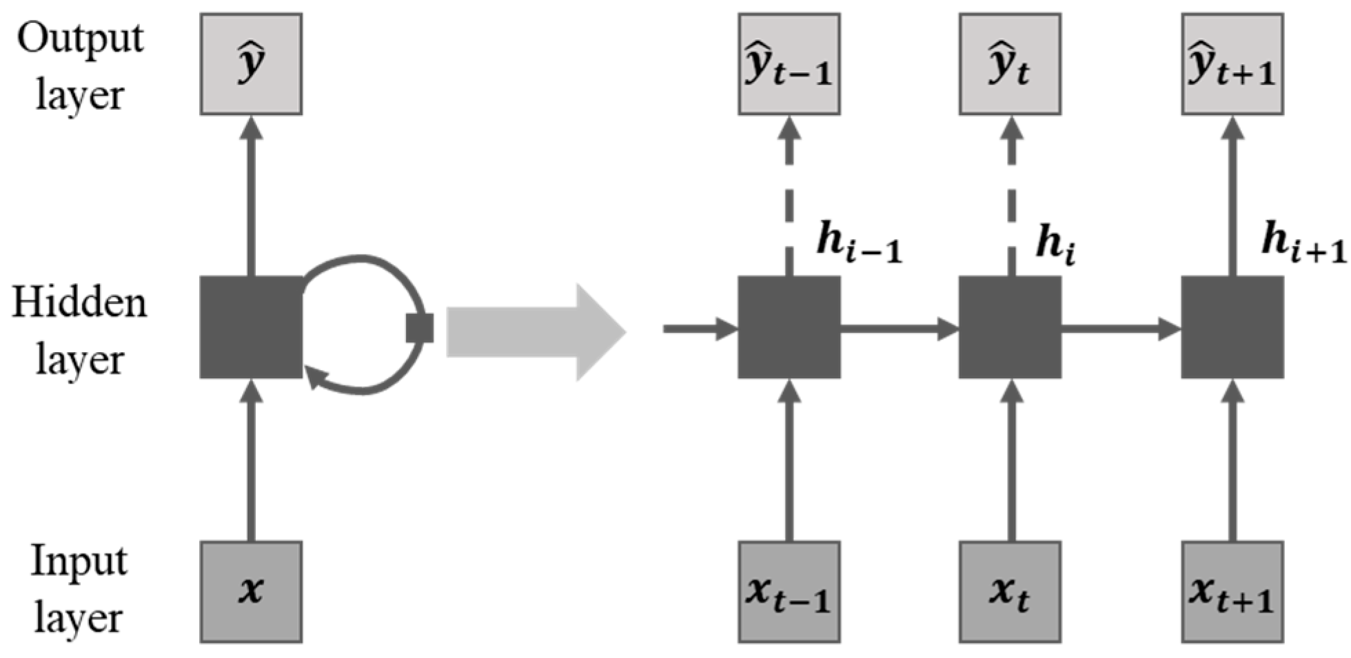
2.2. Recurrent Neural Network
2.3. Ensemble Empirical Mode Decomposition
- 1.
- Add the white noise into the original data to get the new construction:
- 2.
- Describes the time series which have been added the white noise into nth IMF and a residue EMD, .
- 3.
- Repeat steps 1 and 2 M-times with different white noises until you get the appropriate decomposition result.
- 4.
- Calculate the average of the IMF trials which conducted by M-times as the final IMF.
- —number of ensemble members
- —amplitude of the added noises series amplitude
- —final standard deviation of error
- —also interpreted as the difference between the input signal and the relevant IMF [32].
2.4. Wavelet Transformation
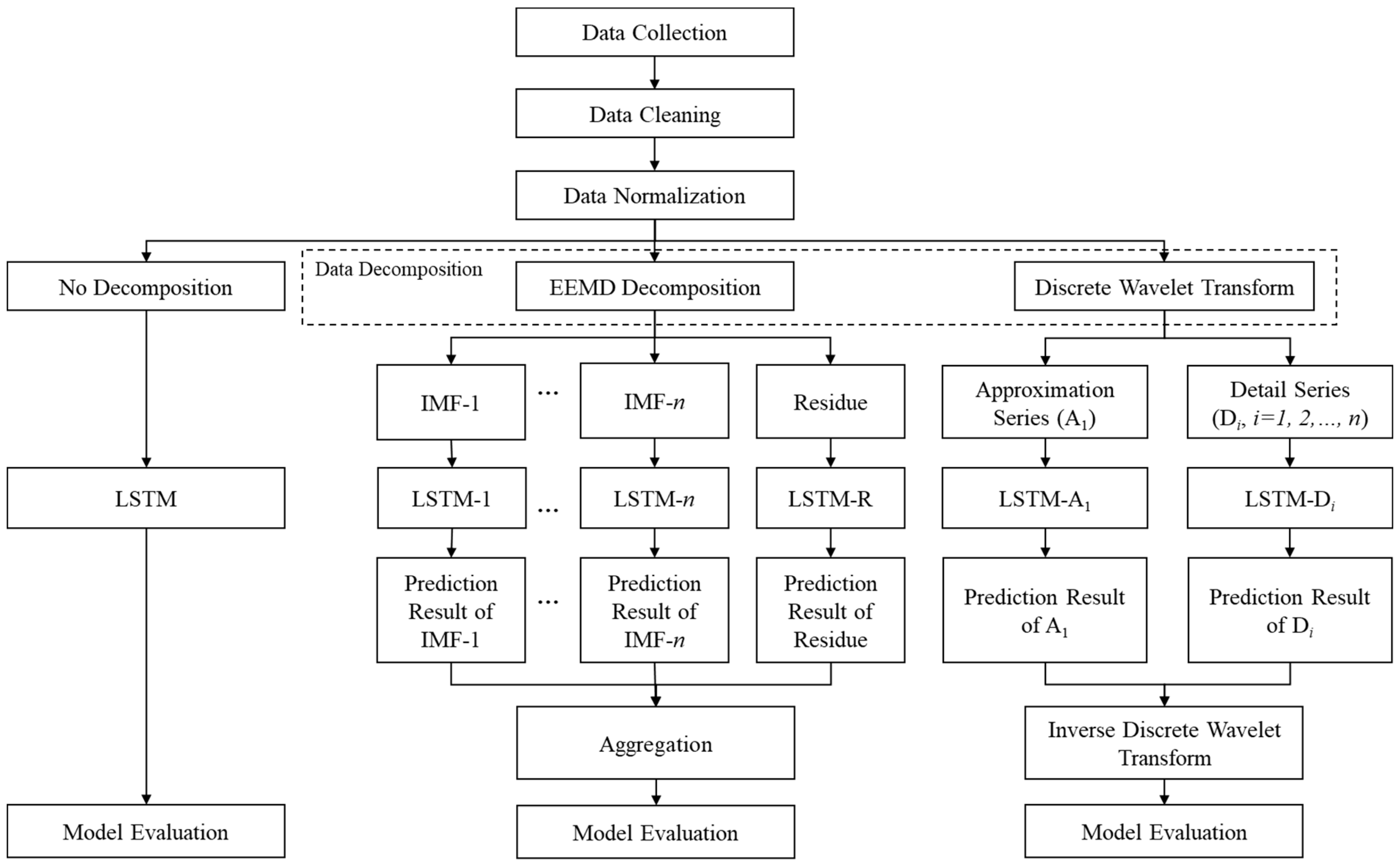
3. Methodology
3.1. Data Pre-Processing
3.1.1. Data Normalization
3.1.2. Statistics Descriptive Analysis
3.1.3. Data Decomposition
- Wavelet Transformation
- 2.
- Ensemble Empirical Mode Decomposition
- (1)
- Add the White Gaussian Noise series into the train set and become the new series of
- (2)
- Decomposed the into several IMFs and a residue .
- (3)
- Then, repeated the steps 1 and 2 on each by adding the white Gaussian noise series for every repeated process. are the amount of repetition.
- (4)
- Take the average of all IMFs and the average of the residue as the final results.
- (5)
- The time series data after EEMD is the sum of all IMFs components and residues as shown in Equation (14).
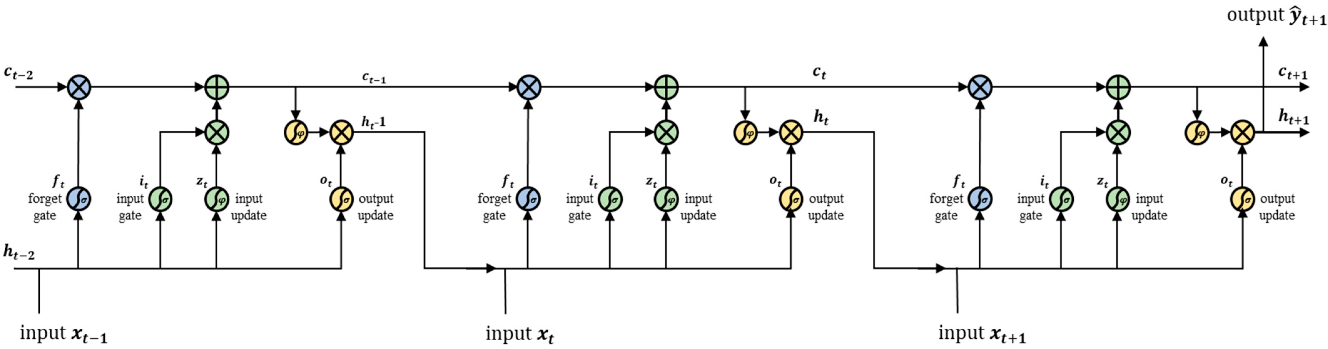
3.2. Forecasting Using LSTM Algorithm
4. Experimental Result
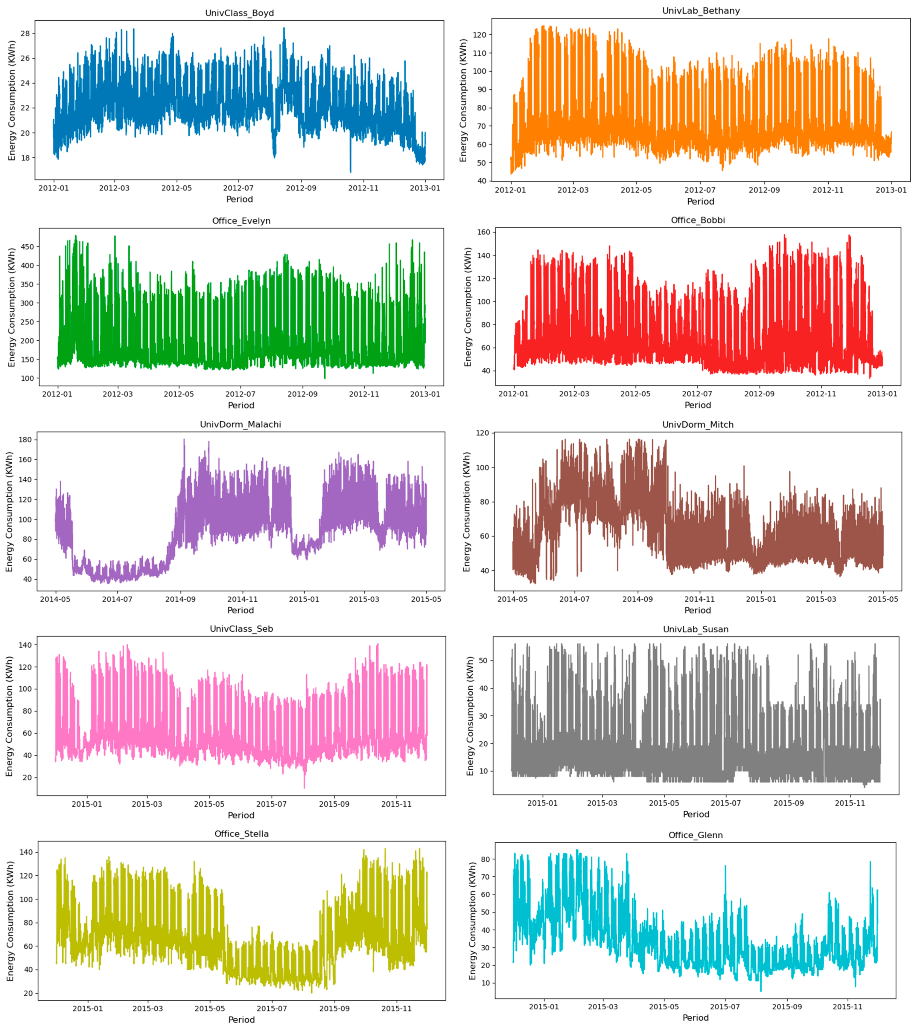
4.1. Dataset Description
4.2. Statistic Description Analysis
- Case 1: KPSS and ADF tests are non-stationary, then the series is non-stationary.
- Case 2: KPSS and ADF tests are stationary, so the series is stationary.
- Case 3: KPSS test is stationary, and ADF is non-stationary, then the series is trend-stationary. The treatment must be done by eliminating the trend to make the series stationary.
- Case 4: KPSS is non-stationary, and ADF is stationary, so the series the difference stationary. Differentiation is used to create a stationary series.
4.3. Parameter Setting
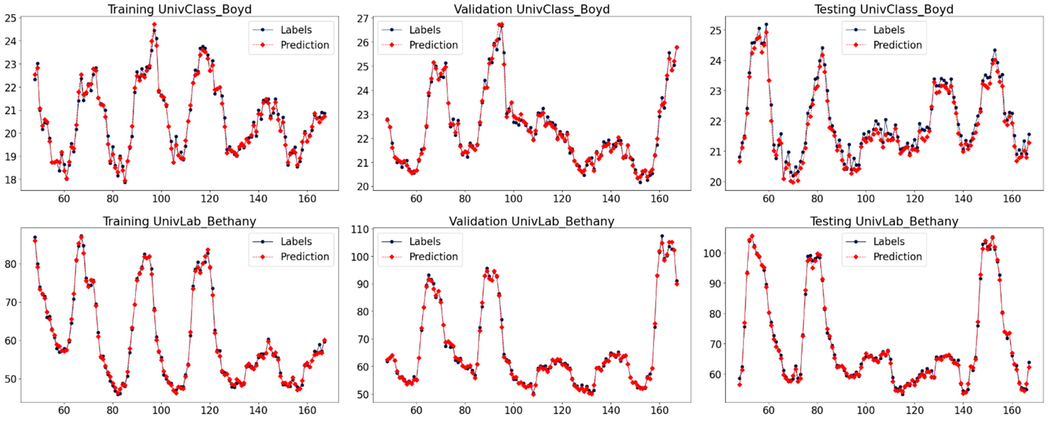
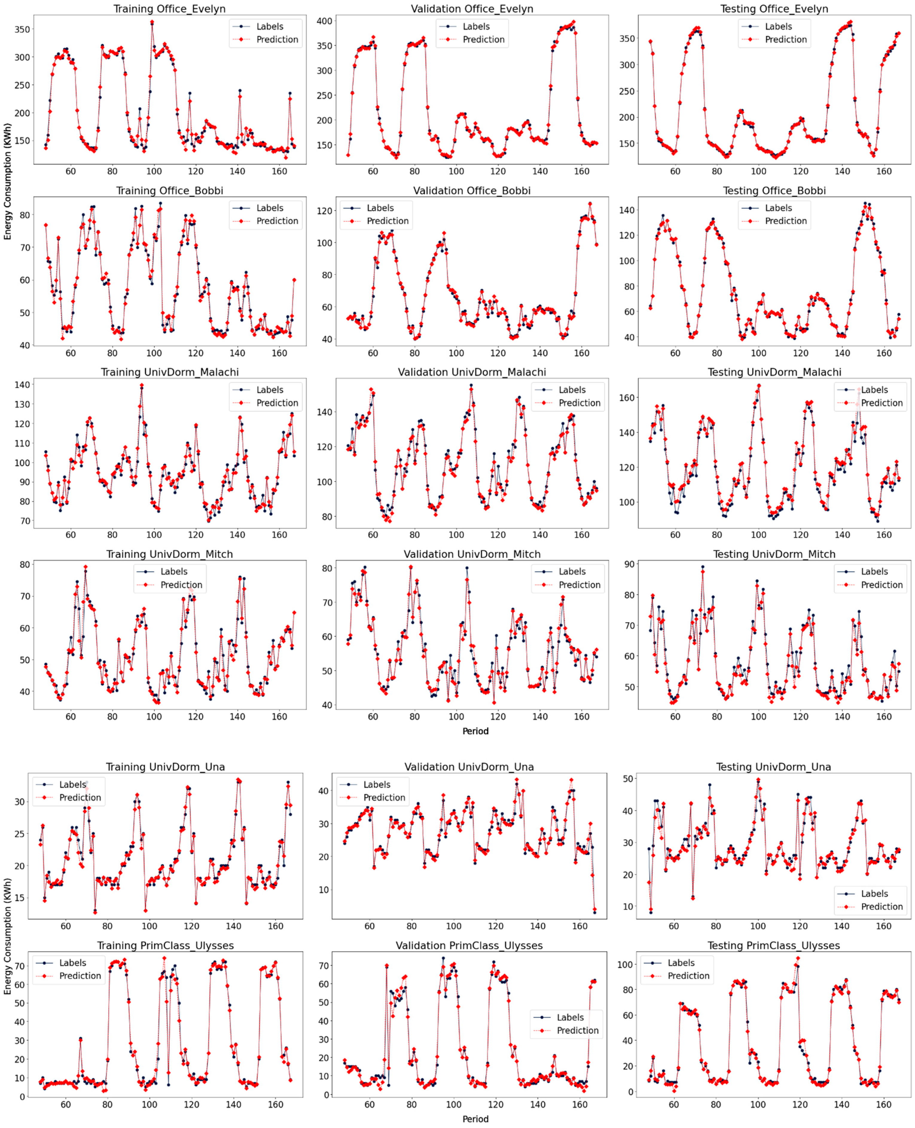
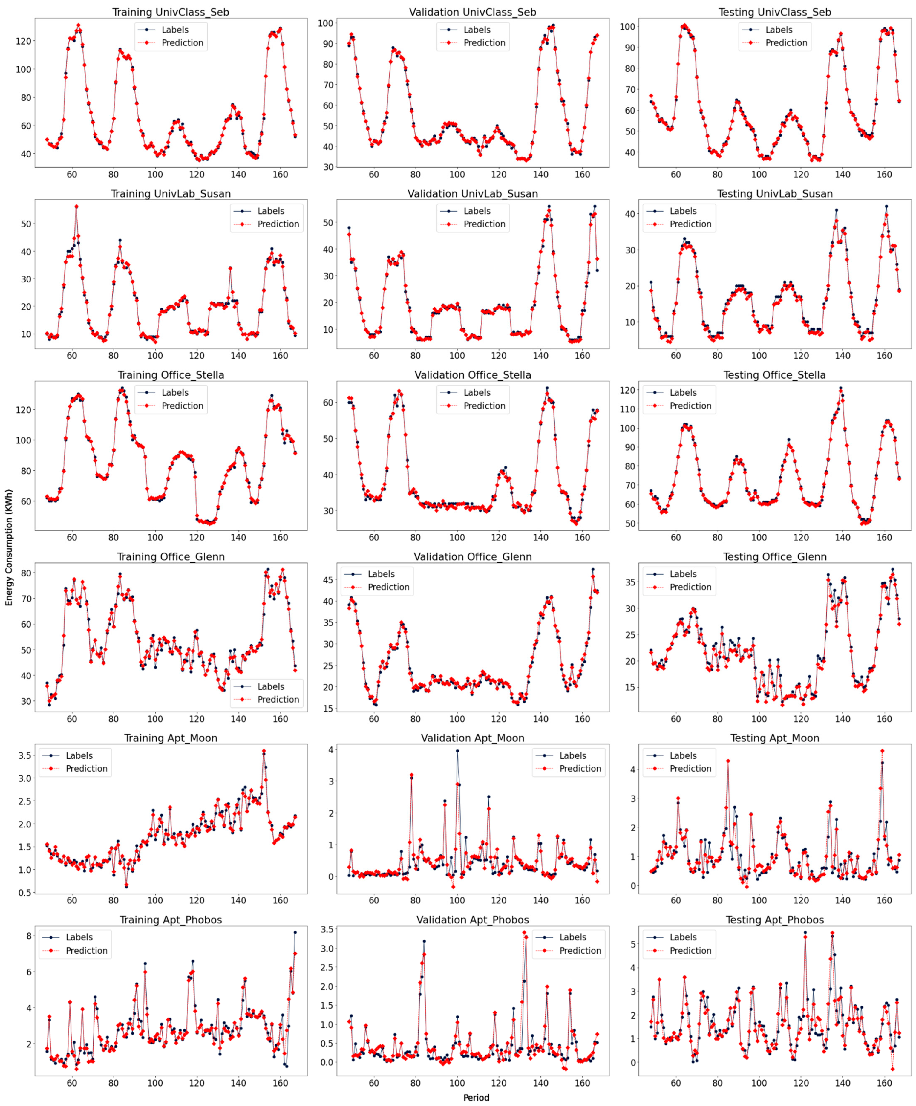
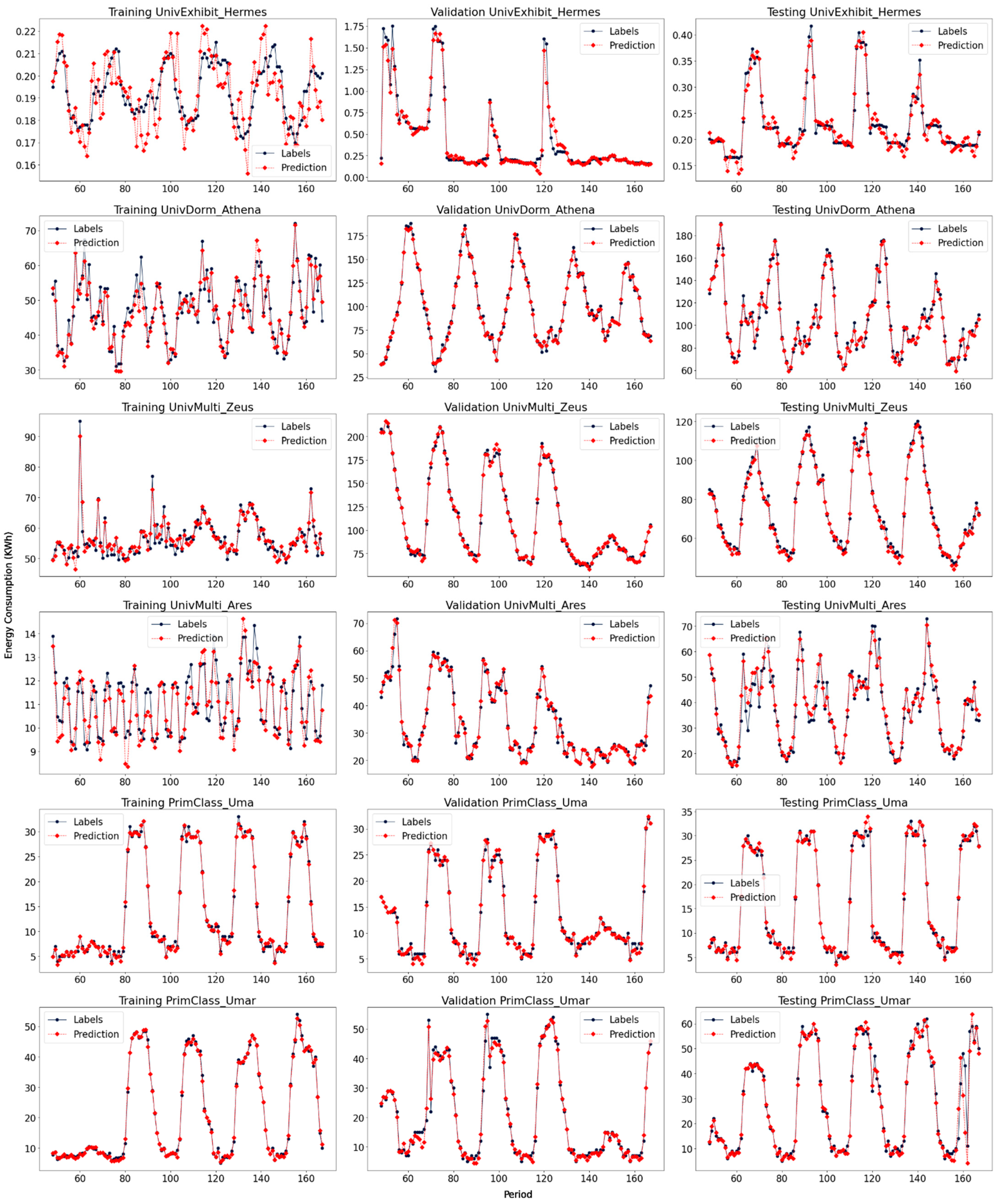
4.4. Forecasting Results Analysis
5. Conclusions
Author Contributions
Funding
Institutional Review Board Statement
Informed Consent Statement
Data Availability Statement
Acknowledgments
Conflicts of Interest
References
- Cao, X.; Dai, X.; Liu, J. Building energy-consumption status worldwide and the state-of-the-art technologies for zero-energy buildings during the past decade. Energy Build. 2016, 128, 198–213. [Google Scholar] [CrossRef]
- Saidur, R.; Masjuki, H.H.; Jamaluddin, M.Y. An application of energy and exergy analysis in residential sector of Malaysia. Energy Policy 2007, 35, 1050–1063. [Google Scholar] [CrossRef]
- Allouhi, A.; El Fouih, Y.; Kousksou, T.; Jamil, A.; Zeraouli, Y.; Mourad, Y. Energy consumption and efficiency in buildings: Current status and future trends. J. Clean. Prod. 2015, 109, 118–130. [Google Scholar] [CrossRef]
- EIA. International Energy Outlook 2019; U.S. Energy Information Administration (EIA): Washington, DC, USA, 2019.
- Bedi, J.; Toshniwal, D. Empirical mode decomposition based deep learning for electricity demand forecasting. IEEE Access 2018, 6, 49144–49156. [Google Scholar] [CrossRef]
- Ahmad, T.; Chen, H. A review on machine learning forecasting growth trends and their real-time applications in different energy systems. Sustain. Cities Soc. 2020, 54, 102010. [Google Scholar] [CrossRef]
- Kontokosta, C.E.; Tull, C. A data-driven predictive model of city-scale energy use in buildings. Appl. Energy 2017, 197, 303–317. [Google Scholar] [CrossRef] [Green Version]
- Hong, W.-C.; Dong, Y.; Zhang, W.Y.; Chen, L.-Y.; Panigrahi, B.K. Cyclic electric load forecasting by seasonal SVR with chaotic genetic algorithm. Int. J. Electr. Power Energy Syst. 2013, 44, 604–614. [Google Scholar] [CrossRef]
- Kneifel, J.; Webb, D. Predicting energy performance of a net-zero energy building: A statistical approach. Appl. Energy 2016, 178, 468–483. [Google Scholar] [CrossRef] [PubMed] [Green Version]
- Barhmi, S.; Elfatni, O.; Belhaj, I. Forecasting of wind speed using multiple linear regression and artificial neural networks. Energy Syst. 2019, 11, 935–946. [Google Scholar] [CrossRef]
- Montgomery, D.; Jennings, C.; Kulahci, M. Introduction to Time Series Analysis and Forecasting; John Wiley & Sons: Hoboken, NJ, USA, 2008; p. 472. [Google Scholar]
- Mocanu, E.; Nguyen, P.H.; Gibescu, M.; Kling, W.L. Deep learning for estimating building energy consumption. Sustain. Energy Netw. 2016, 6, 91–99. [Google Scholar] [CrossRef]
- Kong, W.; Dong, Z.Y.; Jia, Y.; Hill, D.J.; Xu, Y.; Zhang, Y. Short-term residential load forecasting based on lstm recurrent neural network. IEEE Trans. Smart Grid 2019, 10, 841–885. [Google Scholar] [CrossRef]
- Fang, C.; Gao, Y.; Ruan, Y. Improving forecasting accuracy of daily energy consumption of office building using time series analysis based on wavelet transform decomposition. IOP Conf. Ser. Earth Environ. Sci. 2019, 294, 012031. [Google Scholar] [CrossRef] [Green Version]
- Peng, L.; Wang, L.; Xia, D.; Gao, Q.J.E. Effective energy consumption forecasting using empirical wavelet transform and long short-term memory. Energy 2022, 238, 121756. [Google Scholar] [CrossRef]
- Gao, Y.; Ruan, Y.J.E. Buildings, interpretable deep learning model for building energy consumption prediction based on attention mechanism. Energy Build. 2021, 252, 111379. [Google Scholar] [CrossRef]
- Somu, N.; MR, G.R.; Ramamritham, K.J.A.E. A hybrid model for building energy consumption forecasting using long short term memory networks. Appl. Energy 2020, 261, 114131. [Google Scholar] [CrossRef]
- Runge, J.; Zmeureanu, R. Forecasting energy use in buildings using artificial neural networks: A review. Energies 2019, 12, 3254. [Google Scholar] [CrossRef] [Green Version]
- Box, G.E.; Jenkins, G.M.; Reinsel, G.C.; Ljung, G.M. Time Series Analysis: Forecasting and Control; John Wiley & Sons: Hoboken, NJ, USA, 2015. [Google Scholar]
- Koprinska, I.; Rana, M.; Agelidis, V.G. Correlation and instance based feature selection for electricity load forecasting. Knowl.-Based Sys. 2015, 82, 29–40. [Google Scholar] [CrossRef]
- Friedrich, L.; Afshari, A. Short-term forecasting of the abu dhabi electricity load using multiple weather variables. Energy Procedia 2015, 75, 3014–3026. [Google Scholar] [CrossRef] [Green Version]
- Deb, C.; Zhang, F.; Yang, J.; Lee, S.E.; Shah, K.W. A review on time series forecasting techniques for building energy consumption. Renew. Sustain. Energy Rev. 2017, 74, 902–924. [Google Scholar] [CrossRef]
- Bourdeau, M.; Zhai, X.; Nefzaoui, E.; Guo, X.; Chatellier, P. Modeling and forecasting building energy consumption: A review of data-driven techniques. Sustain. Cities Soc. 2019, 48, 101533. [Google Scholar] [CrossRef]
- Mandic, D.P.; Chambers, J.A. Recurrent Neural Networks for Prediction: Learning Algorithms, Architectures and Stability; Wiley: Hoboken, NJ, USA, 2001. [Google Scholar]
- Kumar, D.N.; Raju, K.S.; Sathish, T. River flow forecasting using recurrent neural networks. Water Resour. Manag. 2004, 18, 143–161. [Google Scholar] [CrossRef]
- Hua, Y.; Zhao, Z.; Li, R.; Chen, X.; Liu, Z.; Zhang, H. Deep learning with long short-term memory for time series prediction. IEEE Commun Mag. 2019, 57, 114–119. [Google Scholar] [CrossRef] [Green Version]
- Rumelhart, D.E.; Hinton, G.E.; Williams, R.J. Learning representations by back-propagating errors. Nature 1986, 323, 533–536. [Google Scholar] [CrossRef]
- Hochreiter, S.; Schmidhuber, J. Long Short-Term Memory. Neural Comput. 1997, 9, 1735–1780. [Google Scholar] [CrossRef]
- Aungiers, J. LSTM Neural Network for Time Series Prediction. Available online: https://www.jakob-aungiers.com/articles/a/LSTM-Neural-Network-for-Time-Series-Prediction (accessed on 13 March 2021).
- Wu, Y.-X.; Wu, Q.-B.; Zhu, J.-Q. Improved EEMD-based crude oil price forecasting using LSTM networks. Phys. A Stat. Mech. its Appl. 2019, 516, 114–124. [Google Scholar] [CrossRef]
- Xu, Y.; Zhou, C.; Geng, J.; Gao, S.; Wang, P. A method for diagnosing mechanical faults of on-load tap changer based on ensemble empirical mode decomposition, volterra model and decision acyclic graph support vector machine. IEEE Access 2019, 7, 84803–84816. [Google Scholar] [CrossRef]
- Wu, Z.; Huang, N.E. Ensemble empirical mode decomposition: A noise-assisted data analysis method. Adv. Adapt. Data Anal. 2009, 1, 1–41. [Google Scholar] [CrossRef]
- Huang, N.; Shen, Z.; Long, S. A new view of non-linear water waves: The hilbert spectrum. Annu. Rev. Fluid Mech. 2003, 31, 417–457. [Google Scholar] [CrossRef] [Green Version]
- Zhang, X.; Lai, K.K.; Wang, S.-Y. A new approach for crude oil price analysis based on empirical mode decomposition. Energy Econ. 2008, 30, 905–918. [Google Scholar] [CrossRef]
- Terzija, N. Robust Digital Image Watermarking Algorithms for Copyright Protection. Ph.D. Thesis, University of Duisburg-Essen, Duisburg, Germany, 2006. [Google Scholar]
- Sripathi, D. Efficient Implementations of Discrete Wavelet Transforms using FPGAs; Florida State University, Florida, USA. 2003. Available online: http://purl.flvc.org/fsu/fd/FSU_migr_etd-1599 (accessed on 18 July 2021).
- Sugiartawan, P.; Pulungan, R.; Kartika, A. Prediction by a hybrid of wavelet transform and long-short-term-memory neural networks. Int. J. Adv. Comput. Sci. Appl. 2017, 8, e0142064. [Google Scholar] [CrossRef] [Green Version]
- Jin, J.; Kim, J. Forecasting natural gas prices using wavelets, time series, and artificial neural networks. PLoS ONE 2015, 10, e0142064. [Google Scholar] [CrossRef]
- Chang, Z.; Zhang, Y.; Chen, W. Electricity price prediction based on hybrid model of adam optimized LSTM neural network and wavelet transform. Energy 2019, 187, 115804. [Google Scholar] [CrossRef]
- Liu, Y.; Guan, L.; Hou, C.; Han, H.; Liu, Z.; Sun, Y.; Zheng, M. Wind Power Short-Term Prediction Based on LSTM and Discrete Wavelet Transform. Appl. Sci. 2019, 9, 1108. [Google Scholar] [CrossRef] [Green Version]
- Wang, F.; Yu, Y.; Zhang, Z.; Li, J.; Zhen, Z.; Li, K. Wavelet decomposition and convolutional lstm networks based improved deep learning model for solar irradiance forecasting. Appl. Sci. 2018, 8, 1286. [Google Scholar] [CrossRef] [Green Version]
- Qin, Q.; Lai, X.; Zou, J. Direct multistep wind speed forecasting using lstm neural network combining eemd and fuzzy entropy. Appl. Sci. 2019, 9, 126. [Google Scholar] [CrossRef] [Green Version]
- Liu, W.; Liu, W.D.; Gu, J. Forecasting oil production using ensemble empirical model decomposition based long short-term memory neural network. J. Pet. Sci. Eng. 2020, 189, 107013. [Google Scholar] [CrossRef]
- Miller, C.; Meggers, F. The building data genome project: An open, public data set from non-residential building electrical meters. Energy Procedia 2017, 122, 439–444. [Google Scholar] [CrossRef]
- Barker, S.; Mishra, A.; Irwin, D.; Cecchet, E.; Shenoy, P.; Albrecht, J. Smart*: An open data set and tools for enabling research in sustainable homes. SustKDD 2012, 111, 108. [Google Scholar]
- Kwiatkowski, D.; Phillips, P.C.; Schmidt, P.; Shin, Y. Testing the null hypothesis of stationarity against the alternative of a unit root: How sure are we that economic time series have a unit root? J. Econ. 1992, 54, 159–178. [Google Scholar] [CrossRef]
- Singh, A.A. Gentle Introduction to Handling a Non-Stationary Time Series in Python. Available online: https://www.analyticsvidhya.com/blog/2018/09/non-stationary-time-series-python/# (accessed on 18 July 2021).
- Mueller, J.P.; Massaron, L. Machine Learning for Dummies; John Wiley & Sons: Hoboken, NJ, USA, 2021. [Google Scholar]
- Imani, M.; Ghassemian, H. Lagged load wavelet decomposition and lstm networks for short-term load forecasting. In Proceedings of the 2019 4th International Conference on Pattern Recognition and Image Analysis (IPRIA), Tehran, Iran, 6–7 March 2019; pp. 6–12. [Google Scholar]


| Techniques | Advantages | Disadvantages |
|---|---|---|
| Data-driven | Faster calculations with real-time data | Historical data are needed |
| Can be applied for non-linear problems | Solution for a case may not be suitable for other cases | |
| Deterministic | Refers to the physical science of the building | It is difficult to create scenarios that refer to the actual model |
| Does not require historical data | Requires detail building properties data | |
| One solution can be applied to many cases | - |
| Dataset | Units | Data Start | Data End | Functionalities | Timezone |
|---|---|---|---|---|---|
| 1 | UnivClass_Boyd | 2012-01-01 0:00 | 2012-12-13 23:00 | College Classroom | America/Los_Angeles |
| UnivLab_Bethany | 2012-01-01 0:00 | 2012-12-13 23:00 | College Laboratory | America/Los_Angeles | |
| Office_Evelyn | 2012-01-01 0:00 | 2012-12-13 23:00 | Office | America/Los_Angeles | |
| Office_Bobbi | 2012-01-01 0:00 | 2012-12-13 23:00 | Office | America/Los_Angeles | |
| 2 | UnivDorm_Malachi | 2014-05-01 0:00 | 2015-04-30 23:00 | Residential | America/Chicago |
| UnivDorm_Mitch | 2014-05-01 0:00 | 2015-04-30 23:00 | Residential | America/Chicago | |
| 3 | UnivClass_Seb | 2014-12-01 0:00 | 2015-11-30 23:00 | College Classroom | Europe/London |
| UnivLab_Susan | 2014-12-01 0:00 | 2015-11-30 23:00 | College Laboratory | Europe/London | |
| Office_Stella | 2014-12-01 0:00 | 2015-11-30 23:00 | Office | Europe/London | |
| Office_Glenn | 2014-12-01 0:00 | 2015-11-30 23:00 | Office | Europe/London | |
| 4 | Apt_Moon | 2015-01-01 0:00 | 2015-12-31 23:00 | Apartment | America/New_York |
| Apt_Phobos | 2015-01-01 0:00 | 2015-12-31 23:00 | Apartment | America/New_York | |
| 5 | UnivExhibit_Hermes | 2019-01-02 0:00 | 2020-01-31 23:00 | Exhibition | Asia/Taiwan |
| UnivDorm_Athena | 2019-01-02 0:00 | 2020-01-31 23:00 | Residential | Asia/ Taiwan | |
| UnivMulti_Zeus | 2019-01-02 0:00 | 2020-01-31 23:00 | Multipurpose | Asia/ Taiwan | |
| UnivMulti_Ares | 2019-01-02 0:00 | 2020-01-31 23:00 | Multipurpose | Asia/ Taiwan | |
| 6 | PrimClass_Uma | 2012-02-02 0:00 | 2013-01-31 23:00 | Primary/Secondary Classroom | Asia/Singapore |
| PrimClass_Umar | 2012-02-02 0:00 | 2013-01-31 23:00 | Primary/Secondary Classroom | Asia/Singapore | |
| UnivDorm_Una | 2012-02-02 0:00 | 2013-01-31 23:00 | Residential | Asia/Singapore | |
| PrimClass_Ulysses | 2012-02-02 0:00 | 2013-01-31 23:00 | Primary/Secondary Classroom | Asia/Singapore |
| Dataset | Units | Mean | Stdev | Variance | Min | Max |
|---|---|---|---|---|---|---|
| 1 | UnivClass_Boyd | 22.199 | 1.912 | 3.655 | 16.788 | 28.452 |
| UnivLab_Bethany | 72.946 | 17.247 | 297.451 | 43.634 | 124.788 | |
| Office_Evelyn | 217.398 | 85.811 | 7,363.45 | 98.444 | 479.186 | |
| Office_Bobbi | 74.42 | 28.538 | 814.43 | 33.225 | 157.675 | |
| 2 | UnivDorm_Malachi | 88.061 | 31.071 | 965.429 | 35.25 | 180.25 |
| UnivDorm_Mitch | 62.82 | 17.281 | 298.637 | 32.25 | 116.25 | |
| 3 | UnivClass_Seb | 63.365 | 25.922 | 671.973 | 10 | 141 |
| UnivLab_Susan | 19.157 | 11.801 | 139.27 | 4 | 56 | |
| Office_Stella | 66.442 | 26.473 | 700.829 | 20 | 143 | |
| Office_Glenn | 34.035 | 15.484 | 239.753 | 5.1 | 85.26 | |
| 4 | Apt_Moon | 1.077 | 0.93 | 0.864 | 0.018 | 6.872 |
| Apt_Phobos | 1.382 | 1.241 | 1.539 | 0.012 | 8.715 | |
| 5 | UnivExhibit_Hermes | 0.293 | 0.240 | 0.058 | 0.044 | 2.68 |
| UnivDorm_Athena | 111.908 | 46.138 | 2128.691 | 26.246 | 347.304 | |
| UnivMulti_Zeus | 90.112 | 33.631 | 1131.061 | 35.927 | 222.969 | |
| UnivMulti_Ares | 28.454 | 13.916 | 193.655 | 9.055 | 94.036 | |
| 6 | PrimClass_Uma | 12.375 | 9.01 | 81.184 | 1 | 39 |
| PrimClass_Umar | 21.739 | 17.24 | 297.221 | 1 | 73 | |
| UnivDorm_Una | 23.535 | 8.673 | 75.213 | 1 | 49 | |
| PrimClass_Ulysses | 25.279 | 26.157 | 684.207 | 1 | 103 |
| Series | KPSS Test | ADF Test | Combination of KPSS and ADF Results | ||||
|---|---|---|---|---|---|---|---|
| Test Statistics | p-Value | Interpretation | Test Statistics | p-Value | Interpretation | ||
| UnivClass_Boyd | 1.325 | 0.01 | non-stationary | −7.268 | 1.61 × 10⁻¹⁰ | stationary | difference stationary |
| UnivLab_Bethany | 0.319 | 0.01 | non-stationary | −10.656 | 4.54 × 10⁻¹⁹ | stationary | difference stationary |
| Office_Evelyn | 0.143 | 0.055 | stationary | −13.55 | 2.42 × 10⁻²⁵ | stationary | stationary |
| Office_Bobbi | 0.301 | 0.01 | non-stationary | −10.983 | 7.37 × 10⁻²⁰ | stationary | difference stationary |
| UnivDorm_Malachi | 1.19 | 0.01 | non-stationary | −2.511 | 0.1128005 | non-stationary | non-stationary |
| UnivDorm_Mitch | 1.091 | 0.01 | non-stationary | −3.878 | 0.0022008 | stationary | difference stationary |
| UnivClass_Seb | 0.715 | 0.01 | non-stationary | −11.924 | 4.96 × 10⁻²² | stationary | difference stationary |
| UnivLab_Susan | 0.087 | 0.1 | stationary | −11.191 | 2.36 × 10⁻²⁰ | stationary | stationary |
| Office_Stella | 2.471 | 0.01 | non-stationary | −5.587 | 1.36 × 10⁻⁶ | stationary | difference stationary |
| Office_Glenn | 1.63 | 0.01 | non-stationary | −5.76 | 5.70 × 10⁻⁷ | stationary | difference stationary |
| Apt_Moon | 3.329 | 0.01 | non-stationary | −4.209 | 0.000635 | stationary | difference stationary |
| Apt_Phobos | 3.636 | 0.01 | non-stationary | −4.159 | 0.0007739 | stationary | difference stationary |
| UnivExhibit_Hermes | 1.966 | 0.01 | non-stationary | −8.045 | 1.81 × 10⁻¹² | stationary | difference stationary |
| UnivDorm_Athena | 1.805 | 0.01 | non-stationary | −4.727 | 7.49 × 10⁻⁵ | stationary | difference stationary |
| UnivMulti_Zeus | 2.787 | 0.01 | non-stationary | −6.364 | 2.43 × 10⁻⁸ | stationary | difference stationary |
| UnivMulti_Ares | 1.663 | 0.01 | non-stationary | −6.671 | 4.58 × 10⁻⁹ | stationary | difference stationary |
| PrimClass_Uma | 0.232 | 0.01 | non-stationary | −11.223 | 2.00 × 10⁻²⁰ | stationary | difference stationary |
| PrimClass_Umar | 0.119 | 0.1 | stationary | −12.612 | 1.65 × 10⁻²³ | stationary | stationary |
| UnivDorm_Una | 0.577 | 0.01 | non-stationary | −3.643 | 0.0049932 | stationary | difference stationary |
| PrimClass_Ulysses | 0.216 | 0.01 | non-stationary | −11.645 | 2.11 × 10⁻²¹ | stationary | difference stationary |
| Combinations | Hidden Nodes | Look Back | Activation | Recurrent Activation |
|---|---|---|---|---|
| 1 | 64 | 24 | sigmoid | sigmoid |
| 2 | 64 | 24 | sigmoid | relu |
| 3 | 64 | 24 | sigmoid | tanh |
| 4 | 64 | 24 | tanh | Sigmoid |
| 5 | 64 | 24 | tanh | relu |
| 6 | 64 | 24 | tanh | tanh |
| 7 | 64 | 24 | relu | sigmoid |
| 8 | 64 | 24 | relu | tanh |
| 9 | 64 | 168 | sigmoid | sigmoid |
| 10 | 64 | 168 | sigmoid | tanh |
| 11 | 64 | 168 | tanh | Sigmoid |
| 12 | 64 | 168 | tanh | tanh |
| 13 | 128 | 24 | sigmoid | sigmoid |
| 14 | 128 | 24 | sigmoid | relu |
| 15 | 128 | 24 | sigmoid | tanh |
| 16 | 128 | 24 | tanh | Sigmoid |
| 17 | 128 | 24 | tanh | relu |
| 18 | 128 | 24 | tanh | tanh |
| 19 | 128 | 24 | relu | sigmoid |
| 20 | 128 | 24 | relu | tanh |
| 21 | 128 | 168 | sigmoid | sigmoid |
| 22 | 128 | 168 | sigmoid | tanh |
| 23 | 128 | 168 | tanh | Sigmoid |
| 24 | 128 | 168 | tanh | tanh |
| Parameters | Values |
|---|---|
| Layers | 1 layer |
| Hidden nodes | 64 nodes |
| Look back | 24 h |
| Epochs | 50 epochs |
| Optimizer | Nadam |
| Activation | Tanh |
| Recurrent activation | Sigmoid |
| Dataset | MAPE (%) | MAE | MSE | |||||||
|---|---|---|---|---|---|---|---|---|---|---|
| Metrics | Train | Val | Test | Train | Val | Test | Train | Val | Test | |
| Univclass_Boyd | mean | 1.95 | 1.89 | 2.08 | 0.44 | 0.43 | 0.43 | 0.34 | 0.31 | 0.32 |
| std | 0.02 | 0.02 | 0.10 | 0.00 | 0.01 | 0.02 | 0.00 | 0.01 | 0.02 | |
| Univlab_Bethany | mean | 2.78 | 3.00 | 2.80 | 2.11 | 2.19 | 2.05 | 9.14 | 9.67 | 8.58 |
| std | 0.04 | 0.04 | 0.04 | 0.03 | 0.03 | 0.03 | 0.20 | 0.42 | 0.31 | |
| Office_Evelyn | mean | 4.61 | 4.63 | 6.01 | 10.05 | 10.10 | 13.12 | 438.18 | 352.39 | 674.85 |
| std | 0.14 | 0.32 | 0.12 | 0.28 | 0.71 | 0.23 | 17.13 | 48.76 | 17.05 | |
| Office_Bobbi | mean | 5.72 | 7.87 | 7.83 | 4.29 | 5.18 | 5.40 | 36.75 | 48.39 | 53.76 |
| std | 0.08 | 0.25 | 0.17 | 0.05 | 0.13 | 0.11 | 0.90 | 2.03 | 2.06 | |
| Univdorm_Malachi | mean | 4.76 | 4.71 | 5.77 | 3.78 | 4.86 | 6.32 | 35.43 | 47.07 | 68.26 |
| std | 0.08 | 0.11 | 0.12 | 0.05 | 0.08 | 0.10 | 0.55 | 0.85 | 1.99 | |
| Univdorm_Mitch | mean | 8.10 | 7.98 | 7.85 | 5.74 | 4.55 | 4.53 | 63.85 | 39.92 | 38.46 |
| std | 0.08 | 0.31 | 0.19 | 0.04 | 0.18 | 0.12 | 0.85 | 2.65 | 2.42 | |
| Univclass_Seb | mean | 3.64 | 4.75 | 3.97 | 2.18 | 2.40 | 2.58 | 8.64 | 11.63 | 12.99 |
| std | 0.09 | 0.25 | 0.11 | 0.05 | 0.12 | 0.07 | 0.39 | 1.02 | 0.86 | |
| Univlab_Susan | mean | 7.60 | 13.65 | 11.11 | 1.68 | 2.60 | 1.97 | 9.89 | 21.04 | 11.58 |
| std | 0.58 | 0.67 | 0.85 | 0.07 | 0.09 | 0.12 | 0.46 | 0.92 | 0.71 | |
| Office_Stella | mean | 3.49 | 5.32 | 4.07 | 2.36 | 2.26 | 3.12 | 12.39 | 11.29 | 19.02 |
| std | 0.07 | 0.27 | 0.12 | 0.05 | 0.07 | 0.10 | 0.63 | 0.44 | 1.11 | |
| Office_Glenn | mean | 6.77 | 6.71 | 7.71 | 2.84 | 1.63 | 2.09 | 16.74 | 5.80 | 8.60 |
| std | 0.10 | 0.36 | 0.16 | 0.03 | 0.07 | 0.03 | 0.18 | 0.31 | 0.20 | |
| Apt_Moon | mean | 34.31 | 128.03 | 39.38 | 0.21 | 0.34 | 0.54 | 0.16 | 0.43 | 0.73 |
| std | 2.32 | 10.51 | 0.93 | 0.00 | 0.00 | 0.01 | 0.00 | 0.01 | 0.01 | |
| Apt_Phobos | mean | 47.92 | 116.12 | 49.06 | 0.42 | 0.38 | 0.76 | 0.58 | 0.40 | 1.09 |
| std | 5.82 | 13.42 | 1.26 | 0.00 | 0.00 | 0.00 | 0.01 | 0.01 | 0.01 | |
| Univexhibit_Hermes | mean | 5.95 | 9.27 | 4.98 | 0.02 | 0.05 | 0.01 | 0.01 | 0.02 | 0.00 |
| std | 0.12 | 0.27 | 0.16 | 0.00 | 0.00 | 0.00 | 0.00 | 0.00 | 0.00 | |
| Univdorm_Athena | mean | 8.05 | 8.35 | 9.69 | 8.40 | 9.33 | 8.32 | 120.67 | 155.49 | 117.45 |
| std | 0.12 | 0.19 | 0.24 | 0.12 | 0.24 | 0.13 | 3.35 | 7.31 | 3.10 | |
| Univmulti_Zeus | mean | 5.29 | 5.66 | 8.02 | 5.15 | 5.18 | 5.42 | 53.82 | 57.52 | 66.14 |
| std | 0.10 | 0.20 | 0.68 | 0.05 | 0.13 | 0.32 | 0.54 | 2.40 | 2.78 | |
| Univmulti_Ares | mean | 7.36 | 11.21 | 15.42 | 1.74 | 4.01 | 5.38 | 9.30 | 34.07 | 57.41 |
| std | 0.17 | 0.19 | 0.25 | 0.03 | 0.05 | 0.07 | 0.20 | 1.02 | 1.33 | |
| Primclass_Uma | mean | 19.69 | 17.90 | 17.27 | 1.53 | 1.58 | 1.56 | 10.11 | 8.45 | 9.41 |
| std | 0.45 | 0.64 | 0.56 | 0.03 | 0.04 | 0.04 | 0.28 | 0.41 | 0.46 | |
| Primclass_Umar | mean | 20.59 | 14.96 | 24.42 | 2.67 | 2.73 | 3.84 | 29.92 | 24.17 | 41.45 |
| std | 0.73 | 0.60 | 0.71 | 0.07 | 0.07 | 0.07 | 0.79 | 1.40 | 1.16 | |
| Univdorm_Una | mean | 18.33 | 15.33 | 16.71 | 2.29 | 3.64 | 3.35 | 15.76 | 28.33 | 25.60 |
| std | 0.43 | 0.69 | 0.36 | 0.04 | 0.19 | 0.10 | 0.49 | 3.15 | 1.63 | |
| Primclass_Ulysses | mean | 27.09 | 22.96 | 28.85 | 3.33 | 4.67 | 5.24 | 66.45 | 88.19 | 99.04 |
| std | 0.91 | 0.77 | 0.65 | 0.09 | 0.19 | 0.12 | 1.44 | 4.82 | 2.22 | |
| Dataset | MAPE (%) | MAE | MSE | |||||||
|---|---|---|---|---|---|---|---|---|---|---|
| Metrics | Train | Val | Test | Train | Val | Test | Train | Val | Test | |
| Univclass_Boyd | mean | 1.76 | 2.05 | 2.20 | 0.40 | 0.47 | 0.46 | 0.29 | 0.36 | 0.35 |
| std | 0.03 | 0.02 | 0.05 | 0.01 | 0.01 | 0.01 | 0.01 | 0.00 | 0.01 | |
| Univlab_Bethany | mean | 2.73 | 3.03 | 2.94 | 2.06 | 2.21 | 2.15 | 8.77 | 9.51 | 8.99 |
| std | 0.08 | 0.08 | 0.07 | 0.05 | 0.05 | 0.05 | 0.31 | 0.41 | 0.53 | |
| Office_Evelyn | mean | 4.54 | 4.07 | 6.40 | 9.69 | 8.70 | 13.80 | 401.08 | 192.37 | 692.24 |
| std | 0.10 | 0.25 | 0.14 | 0.24 | 0.64 | 0.25 | 13.18 | 24.36 | 27.48 | |
| Office_Bobbi | mean | 5.47 | 8.10 | 8.02 | 4.07 | 5.27 | 5.50 | 33.29 | 48.61 | 54.71 |
| std | 0.13 | 0.47 | 0.32 | 0.07 | 0.20 | 0.15 | 0.90 | 2.75 | 2.25 | |
| Univdorm_Malachi | mean | 4.75 | 4.94 | 6.05 | 3.71 | 5.12 | 6.65 | 33.93 | 51.35 | 75.23 |
| std | 0.16 | 0.15 | 0.14 | 0.08 | 0.13 | 0.14 | 1.05 | 1.79 | 2.95 | |
| Univdorm_Mitch | mean | 7.51 | 8.51 | 8.39 | 5.27 | 4.83 | 4.81 | 56.00 | 44.73 | 42.79 |
| std | 0.14 | 0.28 | 0.11 | 0.09 | 0.15 | 0.07 | 1.52 | 2.30 | 1.23 | |
| Univclass_Seb | mean | 3.69 | 4.93 | 4.11 | 2.23 | 2.51 | 2.68 | 8.97 | 12.88 | 14.04 |
| std | 0.27 | 0.26 | 0.26 | 0.15 | 0.12 | 0.15 | 0.94 | 0.98 | 1.09 | |
| Univlab_Susan | mean | 7.76 | 13.98 | 10.54 | 1.66 | 2.59 | 1.88 | 9.15 | 20.25 | 10.53 |
| std | 0.35 | 0.81 | 0.66 | 0.04 | 0.07 | 0.06 | 0.35 | 0.64 | 0.46 | |
| Office_Stella | mean | 3.33 | 5.37 | 4.02 | 2.24 | 2.25 | 3.09 | 10.67 | 10.93 | 18.45 |
| std | 0.08 | 0.32 | 0.10 | 0.04 | 0.11 | 0.08 | 0.38 | 0.77 | 0.72 | |
| Office_Glenn | mean | 6.54 | 7.52 | 8.34 | 2.69 | 1.77 | 2.23 | 15.33 | 6.48 | 9.48 |
| std | 0.33 | 1.09 | 0.58 | 0.10 | 0.18 | 0.11 | 0.75 | 0.68 | 0.50 | |
| Apt_Moon | mean | 36.55 | 159.74 | 42.12 | 0.21 | 0.36 | 0.55 | 0.15 | 0.43 | 0.74 |
| std | 2.59 | 16.61 | 0.85 | 0.01 | 0.01 | 0.01 | 0.01 | 0.01 | 0.01 | |
| Apt_Phobos | mean | 54.35 | 151.33 | 52.99 | 0.41 | 0.39 | 0.80 | 0.53 | 0.39 | 1.13 |
| std | 8.97 | 23.68 | 1.77 | 0.01 | 0.01 | 0.01 | 0.02 | 0.02 | 0.03 | |
| Univexhibit_Hermes | mean | 6.15 | 9.73 | 5.44 | 0.03 | 0.05 | 0.01 | 0.01 | 0.02 | 0.00 |
| std | 0.11 | 0.15 | 0.17 | 0.00 | 0.00 | 0.00 | 0.00 | 0.00 | 0.00 | |
| Univdorm_Athena | mean | 7.63 | 8.48 | 10.13 | 7.87 | 9.46 | 8.73 | 108.82 | 159.33 | 127.89 |
| std | 0.34 | 0.29 | 0.47 | 0.22 | 0.31 | 0.26 | 4.32 | 9.61 | 7.01 | |
| Univmulti_Zeus | mean | 5.21 | 5.79 | 7.84 | 5.04 | 5.30 | 5.21 | 52.10 | 58.06 | 63.32 |
| std | 0.13 | 0.22 | 0.57 | 0.12 | 0.16 | 0.27 | 1.91 | 2.34 | 2.67 | |
| Univmulti_Ares | mean | 7.35 | 11.59 | 15.58 | 1.70 | 4.12 | 5.44 | 8.73 | 34.78 | 57.09 |
| std | 0.41 | 0.23 | 0.23 | 0.07 | 0.07 | 0.08 | 0.29 | 0.91 | 1.47 | |
| Primclass_Uma | mean | 18.71 | 18.13 | 17.58 | 1.49 | 1.66 | 1.62 | 9.68 | 9.39 | 9.71 |
| std | 0.66 | 0.86 | 0.60 | 0.05 | 0.05 | 0.04 | 0.38 | 0.40 | 0.39 | |
| Primclass_Umar | mean | 19.80 | 15.31 | 26.64 | 2.56 | 2.78 | 3.94 | 28.12 | 24.25 | 42.46 |
| std | 1.02 | 0.73 | 1.23 | 0.10 | 0.11 | 0.13 | 0.56 | 1.09 | 1.24 | |
| Univdorm_Una | mean | 16.60 | 15.87 | 18.10 | 2.00 | 3.78 | 3.63 | 12.95 | 28.49 | 28.56 |
| std | 0.55 | 0.64 | 0.45 | 0.05 | 0.18 | 0.11 | 0.57 | 2.29 | 1.50 | |
| Primclass_Ulysses | mean | 26.55 | 23.11 | 31.51 | 3.22 | 4.71 | 5.32 | 62.17 | 88.43 | 98.03 |
| std | 1.62 | 0.90 | 1.17 | 0.12 | 0.20 | 0.18 | 1.93 | 3.71 | 3.50 | |
| Dataset | MAPE (%) | MAE | MSE | |||||||
|---|---|---|---|---|---|---|---|---|---|---|
| Metrics | Train | Val | Test | Train | Val | Test | Train | Val | Test | |
| Univclass_Boyd | mean | 0.63 | 0.71 | 1.66 | 0.14 | 0.16 | 0.34 | 0.04 | 0.04 | 0.19 |
| std | 0.01 | 0.04 | 0.12 | 0.00 | 0.01 | 0.02 | 0.00 | 0.00 | 0.03 | |
| Univlab_Bethany | mean | 1.00 | 1.09 | 1.05 | 0.74 | 0.78 | 0.76 | 1.02 | 1.06 | 1.00 |
| std | 0.02 | 0.01 | 0.01 | 0.01 | 0.00 | 0.00 | 0.04 | 0.01 | 0.01 | |
| Office_Evelyn | mean | 1.99 | 1.47 | 2.65 | 4.01 | 3.08 | 5.56 | 49.55 | 17.35 | 113.79 |
| std | 0.04 | 0.01 | 0.02 | 0.08 | 0.03 | 0.02 | 3.20 | 0.24 | 1.50 | |
| Office_Bobbi | mean | 1.90 | 2.30 | 2.43 | 1.36 | 1.50 | 1.65 | 3.25 | 3.85 | 4.90 |
| std | 0.04 | 0.02 | 0.01 | 0.03 | 0.02 | 0.01 | 0.14 | 0.07 | 0.06 | |
| Univdorm_Malachi | mean | 1.95 | 2.36 | 4.80 | 1.43 | 2.22 | 4.97 | 4.22 | 7.71 | 31.57 |
| std | 0.17 | 0.45 | 1.15 | 0.11 | 0.35 | 1.18 | 0.51 | 1.83 | 12.41 | |
| Univdorm_Mitch | mean | 2.75 | 3.00 | 3.52 | 1.89 | 1.64 | 1.95 | 7.58 | 4.96 | 6.12 |
| std | 0.04 | 0.18 | 0.22 | 0.04 | 0.09 | 0.12 | 0.29 | 0.47 | 0.50 | |
| Univclass_Seb | mean | 1.41 | 1.72 | 1.56 | 0.83 | 0.83 | 0.98 | 1.16 | 1.17 | 1.98 |
| std | 0.02 | 0.02 | 0.02 | 0.01 | 0.01 | 0.01 | 0.04 | 0.02 | 0.07 | |
| Univlab_Susan | mean | 4.40 | 7.02 | 9.23 | 0.84 | 1.23 | 1.29 | 1.94 | 4.70 | 2.79 |
| std | 0.26 | 0.37 | 0.95 | 0.06 | 0.05 | 0.12 | 0.26 | 0.07 | 0.34 | |
| Office_Stella | mean | 1.33 | 2.04 | 1.50 | 0.91 | 0.82 | 1.14 | 1.40 | 1.18 | 2.20 |
| std | 0.07 | 0.07 | 0.10 | 0.05 | 0.02 | 0.08 | 0.18 | 0.05 | 0.28 | |
| Office_Glenn | mean | 2.38 | 2.98 | 3.24 | 0.94 | 0.68 | 0.85 | 1.69 | 0.75 | 1.12 |
| std | 0.07 | 0.15 | 0.53 | 0.03 | 0.03 | 0.13 | 0.19 | 0.07 | 0.30 | |
| Apt_Moon | mean | 23.93 | 118.99 | 21.52 | 0.08 | 0.16 | 0.24 | 0.02 | 0.07 | 0.13 |
| std | 1.26 | 0.86 | 0.36 | 0.00 | 0.00 | 0.00 | 0.00 | 0.00 | 0.00 | |
| Apt_Phobos | mean | 34.12 | 70.89 | 19.59 | 0.17 | 0.14 | 0.30 | 0.07 | 0.04 | 0.18 |
| std | 1.14 | 1.72 | 0.11 | 0.00 | 0.00 | 0.01 | 0.00 | 0.00 | 0.01 | |
| Univexhibit_Hermes | mean | 5.24 | 7.91 | 5.20 | 0.01 | 0.02 | 0.01 | 0.00 | 0.00 | 0.00 |
| std | 0.15 | 0.12 | 0.23 | 0.00 | 0.00 | 0.00 | 0.00 | 0.00 | 0.00 | |
| Univdorm_Athena | mean | 2.79 | 2.58 | 5.25 | 2.85 | 2.88 | 4.40 | 13.05 | 13.86 | 28.51 |
| std | 0.05 | 0.02 | 1.15 | 0.06 | 0.04 | 0.86 | 0.47 | 0.44 | 10.02 | |
| Univmulti_Zeus | mean | 1.83 | 2.53 | 3.11 | 1.71 | 2.20 | 1.98 | 5.26 | 7.98 | 8.44 |
| std | 0.01 | 0.16 | 0.22 | 0.02 | 0.12 | 0.16 | 0.15 | 0.70 | 0.54 | |
| Univmulti_Ares | mean | 3.39 | 4.52 | 6.22 | 0.73 | 1.55 | 1.98 | 1.19 | 5.00 | 7.10 |
| std | 0.08 | 0.10 | 0.33 | 0.02 | 0.02 | 0.07 | 0.07 | 0.08 | 0.38 | |
| Primclass_Uma | mean | 7.03 | 6.76 | 6.84 | 0.65 | 0.67 | 0.69 | 1.67 | 1.49 | 1.48 |
| std | 0.10 | 0.09 | 0.11 | 0.00 | 0.01 | 0.02 | 0.02 | 0.06 | 0.09 | |
| Primclass_Umar | mean | 8.30 | 6.84 | 9.60 | 1.08 | 1.09 | 1.52 | 3.73 | 3.72 | 6.72 |
| std | 0.21 | 0.14 | 0.18 | 0.03 | 0.01 | 0.01 | 0.23 | 0.08 | 0.10 | |
| Univdorm_Una | mean | 5.30 | 4.99 | 5.52 | 0.88 | 1.32 | 1.28 | 2.42 | 4.18 | 4.51 |
| std | 0.12 | 0.06 | 0.25 | 0.02 | 0.01 | 0.04 | 0.09 | 0.25 | 0.22 | |
| Primclass_Ulysses | mean | 11.97 | 10.66 | 15.31 | 1.41 | 1.75 | 2.08 | 7.87 | 10.13 | 13.39 |
| std | 0.31 | 0.62 | 1.60 | 0.03 | 0.08 | 0.18 | 0.34 | 0.52 | 1.06 | |
| Dataset | MAPE (%) | MAE | MSE | |||||||
|---|---|---|---|---|---|---|---|---|---|---|
| Metrics | Train | Val | Test | Train | Val | Test | Train | Val | Test | |
| Univclass_Boyd | mean | 2.27 | 2.13 | 2.32 | 0.52 | 0.49 | 0.49 | 0.45 | 0.41 | 0.43 |
| std | 0.03 | 0.03 | 0.15 | 0.01 | 0.01 | 0.03 | 0.01 | 0.01 | 0.04 | |
| Univlab_Bethany | mean | 3.67 | 3.77 | 3.72 | 2.79 | 2.78 | 2.71 | 17.40 | 16.80 | 15.66 |
| std | 0.13 | 0.06 | 0.08 | 0.09 | 0.04 | 0.02 | 1.40 | 0.64 | 0.61 | |
| Office_Evelyn | mean | 6.93 | 6.46 | 8.52 | 14.94 | 13.87 | 18.26 | 778.93 | 577.21 | 1101.00 |
| std | 0.28 | 0.14 | 0.35 | 0.12 | 0.18 | 0.26 | 27.29 | 48.76 | 16.85 | |
| Office_Bobbi | mean | 7.13 | 8.96 | 9.24 | 5.31 | 5.87 | 6.36 | 53.01 | 64.22 | 76.37 |
| std | 0.50 | 0.52 | 0.51 | 0.30 | 0.17 | 0.17 | 4.16 | 1.83 | 2.95 | |
| Univdorm_Malachi | mean | 5.69 | 5.37 | 6.70 | 4.48 | 5.52 | 7.32 | 46.42 | 59.43 | 92.47 |
| std | 0.12 | 0.04 | 0.11 | 0.11 | 0.02 | 0.16 | 1.74 | 0.43 | 4.79 | |
| Univdorm_Mitch | mean | 8.95 | 8.18 | 8.12 | 6.22 | 4.63 | 4.64 | 71.12 | 40.07 | 39.44 |
| std | 0.05 | 0.09 | 0.09 | 0.04 | 0.03 | 0.04 | 0.77 | 0.32 | 0.23 | |
| Univclass_Seb | mean | 4.95 | 6.38 | 5.58 | 2.93 | 3.27 | 3.58 | 17.13 | 23.83 | 26.35 |
| std | 0.29 | 0.07 | 0.15 | 0.16 | 0.03 | 0.12 | 1.90 | 0.56 | 2.36 | |
| Univlab_Susan | mean | 9.11 | 16.59 | 14.42 | 2.04 | 3.22 | 2.57 | 13.30 | 29.66 | 17.03 |
| std | 0.18 | 0.32 | 0.29 | 0.05 | 0.05 | 0.07 | 0.34 | 0.88 | 0.51 | |
| Office_Stella | mean | 4.93 | 6.94 | 5.58 | 3.28 | 2.95 | 4.24 | 21.66 | 19.04 | 32.83 |
| std | 0.27 | 0.20 | 0.15 | 0.19 | 0.06 | 0.12 | 1.56 | 0.28 | 1.34 | |
| Office_Glenn | mean | 7.91 | 8.01 | 8.89 | 3.31 | 1.98 | 2.44 | 22.41 | 9.12 | 12.21 |
| std | 0.01 | 0.15 | 0.05 | 0.01 | 0.01 | 0.01 | 0.10 | 0.07 | 0.05 | |
| Apt_Moon | mean | 40.73 | 192.76 | 46.55 | 0.23 | 0.38 | 0.57 | 0.18 | 0.46 | 0.77 |
| std | 0.44 | 3.32 | 0.48 | 0.00 | 0.00 | 0.00 | 0.00 | 0.00 | 0.00 | |
| Apt_Phobos | mean | 67.95 | 184.62 | 59.32 | 0.48 | 0.40 | 0.82 | 0.68 | 0.40 | 1.17 |
| std | 4.94 | 15.60 | 1.25 | 0.00 | 0.00 | 0.01 | 0.01 | 0.01 | 0.02 | |
| Univexhibit_Hermes | mean | 10.06 | 15.13 | 7.55 | 0.04 | 0.07 | 0.02 | 0.01 | 0.03 | 0.00 |
| std | 0.25 | 0.06 | 0.04 | 0.00 | 0.00 | 0.00 | 0.00 | 0.00 | 0.00 | |
| Univdorm_Athena | mean | 9.68 | 10.20 | 12.47 | 9.92 | 11.25 | 10.68 | 163.75 | 229.93 | 189.17 |
| std | 0.24 | 0.08 | 0.37 | 0.17 | 0.11 | 0.24 | 4.29 | 3.24 | 8.39 | |
| Univmulti_Zeus | mean | 6.12 | 6.72 | 8.39 | 6.04 | 6.33 | 5.83 | 76.16 | 93.89 | 80.47 |
| std | 0.07 | 0.05 | 0.04 | 0.06 | 0.03 | 0.05 | 0.92 | 0.90 | 1.85 | |
| Univmulti_Ares | mean | 11.57 | 15.12 | 19.66 | 2.60 | 5.32 | 6.81 | 17.10 | 54.41 | 90.39 |
| std | 0.27 | 0.14 | 0.50 | 0.05 | 0.02 | 0.13 | 0.43 | 0.58 | 3.07 | |
| Primclass_Uma | mean | 19.61 | 18.80 | 18.36 | 1.69 | 1.77 | 1.81 | 11.61 | 12.21 | 12.83 |
| std | 0.36 | 0.34 | 0.32 | 0.04 | 0.03 | 0.03 | 0.26 | 0.33 | 0.23 | |
| Primclass_Umar | mean | 22.26 | 17.09 | 28.61 | 3.13 | 3.10 | 4.45 | 32.27 | 29.29 | 47.92 |
| std | 0.81 | 0.43 | 0.49 | 0.08 | 0.03 | 0.01 | 1.14 | 0.72 | 0.16 | |
| Univdorm_Una | mean | 21.54 | 17.96 | 18.51 | 2.92 | 4.31 | 3.82 | 19.63 | 33.75 | 28.21 |
| std | 1.52 | 0.90 | 1.09 | 0.29 | 0.20 | 0.31 | 2.04 | 2.44 | 3.73 | |
| Primclass_Ulysses | mean | 28.72 | 22.05 | 29.78 | 3.65 | 4.59 | 5.38 | 71.42 | 92.63 | 109.26 |
| std | 0.98 | 0.50 | 0.38 | 0.18 | 0.11 | 0.10 | 1.13 | 2.14 | 2.52 | |
| Dataset | Training | Validation | Testing | |||||||||
|---|---|---|---|---|---|---|---|---|---|---|---|---|
| RNN | LSTM | EEMD LSTM | WT LSTM | RNN | LSTM | EEMD LSTM | WT LSTM | RNN | LSTM | EEMD LSTM | WT LSTM | |
| Univclass_Boyd | 1.76 | 1.95 | 0.63 * | 2.27 | 2.05 | 1.89 | 0.71 * | 2.13 | 2.2 | 2.08 | 1.66 * | 2.32 |
| Univlab_Bethany | 2.73 | 2.78 | 1 * | 3.67 | 3.03 | 3 | 1.09 * | 3.77 | 2.94 | 2.8 | 1.05 * | 3.72 |
| Office_Evelyn | 4.54 | 4.61 | 1.99 * | 6.93 | 4.07 | 4.63 | 1.47 * | 6.46 | 6.4 | 6.01 | 2.65 * | 8.52 |
| Office_Bobbi | 5.47 | 5.72 | 1.9 * | 7.13 | 8.1 | 7.87 | 2.3 * | 8.96 | 8.02 | 7.83 | 2.43 * | 9.24 |
| Univdorm_Malachi | 4.75 | 4.76 | 1.95 * | 5.69 | 4.94 | 4.71 | 2.36 * | 5.37 | 6.05 | 5.77 | 4.8 * | 6.7 |
| Univdorm_Mitch | 7.51 | 8.1 | 2.75 * | 8.95 | 8.51 | 7.98 | 3 * | 8.18 | 8.39 | 7.85 | 3.52 * | 8.12 |
| Univclass_Seb | 3.69 | 3.64 | 1.41 * | 4.95 | 4.93 | 4.75 | 1.72 * | 6.38 | 4.11 | 3.97 | 1.56 * | 5.58 |
| Univlab_Susan | 7.76 | 7.6 | 4.4 * | 9.11 | 13.98 | 13.65 | 7.02 * | 16.59 | 10.54 | 11.11 | 9.23 * | 14.42 |
| Office_Stella | 3.33 | 3.49 | 1.33 * | 4.93 | 5.37 | 5.32 | 2.04 * | 6.94 | 4.02 | 4.07 | 1.5 * | 5.58 |
| Office_Glenn | 6.54 | 6.77 | 2.38 * | 7.91 | 7.52 | 6.71 | 2.98 * | 8.01 | 8.34 | 7.71 | 3.24 * | 8.89 |
| Apt_Moon | 36.55 | 34.31 | 23.93 * | 40.73 | 159.74 | 128.03 | 118.9 * | 192.76 | 42.12 | 39.38 | 21.52 * | 46.55 |
| Apt_Phobos | 54.35 | 47.92 | 34.12 * | 67.95 | 151.33 | 116.12 | 70.89 * | 184.62 | 52.99 | 49.06 | 19.59 * | 59.32 |
| Univexhibit_Hermes | 6.15 | 5.95 | 5.24 * | 10.06 | 9.73 | 9.27 | 7.91 * | 15.13 | 5.44 | 4.98 * | 5.2 | 7.55 |
| Univdorm_Athena | 7.63 | 8.05 | 2.79 * | 9.68 | 8.48 | 8.35 | 2.58 * | 10.2 | 10.13 | 9.69 | 5.25 * | 12.47 |
| Univmulti_Zeus | 5.21 | 5.29 | 1.83 * | 6.12 | 5.79 | 5.66 | 2.53 * | 6.72 | 7.84 | 8.02 | 3.11 * | 8.39 |
| Univmulti_Ares | 7.35 | 7.36 | 3.39 * | 11.57 | 11.59 | 11.21 | 4.52 * | 15.12 | 15.58 | 15.42 | 6.22 * | 19.66 |
| Primclass_Uma | 18.71 | 19.69 | 7.03 * | 19.61 | 18.13 | 17.9 | 6.76 * | 18.8 | 17.58 | 17.27 | 6.84 * | 18.36 |
| Primclass_Umar | 19.8 | 20.59 | 8.3 * | 22.26 | 15.31 | 14.96 | 6.84 * | 17.09 | 26.64 | 24.42 | 9.6 * | 28.61 |
| Univdorm_Una | 16.6 | 18.33 | 5.3 * | 21.54 | 15.87 | 15.33 | 4.99 * | 17.96 | 18.1 | 16.71 | 5.52 * | 18.51 |
| Primclass_Ulysses | 26.55 | 27.09 | 11.97 * | 28.72 | 23.11 | 22.96 | 10.66 * | 22.05 | 31.51 | 28.85 | 15.31 * | 29.78 |
| Dataset | MAPE (%) | MAE | MSE | |||||||
|---|---|---|---|---|---|---|---|---|---|---|
| Metrics | Train | Val | Test | Training | Metrics | Train | Val | Test | Testing | |
| Univclass_Boyd | mean | 1.98 | 1.98 | 1.99 | 0.45 | 0.46 | 0.44 | 0.34 | 0.35 | 0.33 |
| std | 0.07 | 0.13 | 0.13 | 0.01 | 0.04 | 0.04 | 0.02 | 0.05 | 0.06 | |
| Univlab_Bethany | mean | 2.96 | 3.06 | 3.08 | 2.24 | 2.32 | 2.28 | 10.52 | 10.84 | 10.39 |
| std | 0.23 | 0.16 | 0.29 | 0.17 | 0.18 | 0.30 | 1.74 | 2.17 | 2.75 | |
| Office_Evelyn | mean | 5.63 | 4.80 | 5.37 | 12.82 | 10.55 | 11.57 | 669.14 | 437.24 | 468.07 |
| std | 1.30 | 2.40 | 1.68 | 3.55 | 5.98 | 3.80 | 296.19 | 523.21 | 320.99 | |
| Office_Bobbi | mean | 5.79 | 6.87 | 7.22 | 4.34 | 5.04 | 5.07 | 38.45 | 48.06 | 47.68 |
| std | 0.13 | 0.91 | 0.81 | 0.16 | 0.71 | 0.53 | 3.48 | 13.67 | 8.96 | |
| Univdorm_Malachi | mean | 4.86 | 5.29 | 5.88 | 3.55 | 4.63 | 5.91 | 30.76 | 45.01 | 72.17 |
| std | 0.52 | 0.80 | 1.18 | 0.68 | 1.72 | 2.15 | 9.96 | 27.51 | 48.69 | |
| Univdorm_Mitch | mean | 8.13 | 8.09 | 8.39 | 5.50 | 5.58 | 5.43 | 60.91 | 58.41 | 56.46 |
| std | 0.61 | 1.08 | 0.92 | 0.24 | 0.99 | 1.08 | 3.79 | 17.42 | 21.47 | |
| Univclass_Seb | mean | 4.28 | 4.53 | 4.64 | 2.55 | 2.72 | 2.71 | 11.97 | 14.12 | 13.77 |
| std | 0.82 | 0.68 | 0.64 | 0.44 | 0.58 | 0.41 | 4.46 | 6.71 | 4.08 | |
| Univlab_Susan | mean | 9.63 | 12.22 | 12.63 | 2.08 | 2.50 | 2.38 | 13.45 | 18.08 | 16.36 |
| std | 2.95 | 2.93 | 2.30 | 0.49 | 0.73 | 0.59 | 5.24 | 10.41 | 8.70 | |
| Office_Stella | mean | 3.89 | 4.66 | 5.73 | 2.66 | 2.72 | 3.19 | 15.49 | 14.90 | 19.74 |
| std | 0.52 | 1.25 | 2.37 | 0.42 | 0.55 | 0.59 | 4.56 | 5.22 | 5.80 | |
| Office_Glenn | mean | 7.19 | 7.30 | 8.49 | 3.19 | 2.54 | 2.47 | 20.13 | 13.62 | 12.25 |
| std | 0.66 | 1.02 | 1.76 | 0.49 | 1.05 | 0.82 | 4.86 | 10.11 | 8.00 | |
| Apt_Moon | mean | 28.05 | 82.00 | 110.99 | 0.23 | 0.31 | 0.38 | 0.15 | 0.32 | 0.43 |
| std | 16.15 | 58.70 | 79.86 | 0.01 | 0.08 | 0.11 | 0.05 | 0.19 | 0.23 | |
| Apt_Phobos | mean | 42.10 | 78.63 | 130.29 | 0.50 | 0.45 | 0.53 | 0.71 | 0.60 | 0.65 |
| std | 17.11 | 48.48 | 117.08 | 0.09 | 0.16 | 0.16 | 0.16 | 0.33 | 0.30 | |
| Univexhibit_Hermes | mean | 5.45 | 8.01 | 9.19 | 0.02 | 0.03 | 0.05 | 0.01 | 0.01 | 0.02 |
| std | 1.34 | 2.83 | 4.45 | 0.01 | 0.03 | 0.04 | 0.01 | 0.01 | 0.02 | |
| Univdorm_Athena | mean | 8.77 | 9.75 | 10.53 | 8.41 | 10.52 | 11.53 | 121.42 | 184.66 | 255.98 |
| std | 1.10 | 2.13 | 1.29 | 0.44 | 1.22 | 2.94 | 11.49 | 36.83 | 165.99 | |
| Univmulti_Zeus | mean | 5.77 | 5.63 | 6.23 | 5.24 | 5.39 | 5.59 | 57.62 | 58.09 | 67.20 |
| std | 0.57 | 0.52 | 1.13 | 0.25 | 0.56 | 0.53 | 6.04 | 11.55 | 15.04 | |
| Univmulti_Ares | mean | 7.59 | 10.44 | 12.37 | 1.62 | 3.22 | 3.99 | 7.68 | 25.13 | 35.01 |
| std | 0.83 | 2.34 | 2.29 | 0.38 | 1.36 | 1.25 | 3.36 | 17.99 | 17.34 | |
| Primclass_Uma | mean | 20.35 | 24.15 | 20.05 | 1.74 | 2.05 | 1.72 | 11.91 | 16.02 | 10.39 |
| std | 1.92 | 12.26 | 3.63 | 0.27 | 0.98 | 0.38 | 2.76 | 14.37 | 4.17 | |
| Primclass_Umar | mean | 19.94 | 23.81 | 22.26 | 2.77 | 3.56 | 3.38 | 29.92 | 45.42 | 36.31 |
| std | 2.05 | 10.09 | 5.26 | 0.27 | 1.20 | 0.47 | 4.99 | 31.71 | 9.52 | |
| Univdorm_Una | mean | 15.99 | 24.26 | 21.37 | 2.32 | 3.46 | 3.45 | 15.69 | 30.04 | 26.86 |
| std | 3.19 | 12.87 | 7.79 | 0.27 | 0.78 | 0.49 | 3.52 | 15.26 | 8.09 | |
| Primclass_Ulysses | mean | 28.54 | 32.62 | 30.10 | 3.95 | 4.90 | 4.75 | 79.57 | 103.86 | 88.49 |
| std | 2.34 | 16.08 | 6.46 | 0.45 | 1.84 | 0.80 | 8.32 | 62.30 | 21.51 | |
| Dataset | MAPE (%) | MAE | MSE | |||||||
|---|---|---|---|---|---|---|---|---|---|---|
| Metrics | Train | Val | Test | Train | Val | Test | Train | Val | Test | |
| Univclass_Boyd | mean | 1.77 | 2.15 | 2.19 | 0.40 | 0.49 | 0.49 | 0.29 | 0.40 | 0.40 |
| std | 0.07 | 0.14 | 0.19 | 0.02 | 0.04 | 0.06 | 0.02 | 0.07 | 0.09 | |
| Univlab_Bethany | mean | 2.89 | 3.16 | 3.25 | 2.17 | 2.38 | 2.40 | 9.93 | 11.15 | 11.05 |
| std | 0.35 | 0.33 | 0.45 | 0.23 | 0.31 | 0.41 | 1.98 | 3.22 | 3.55 | |
| Office_Evelyn | mean | 5.47 | 5.29 | 5.70 | 11.98 | 11.16 | 11.90 | 543.37 | 413.15 | 453.10 |
| std | 1.19 | 2.95 | 2.08 | 2.97 | 6.88 | 4.49 | 198.38 | 495.12 | 346.28 | |
| Office_Bobbi | mean | 5.56 | 7.09 | 7.43 | 4.14 | 5.17 | 5.22 | 35.50 | 49.38 | 49.74 |
| std | 0.20 | 0.91 | 0.69 | 0.14 | 0.78 | 0.50 | 2.45 | 14.41 | 8.89 | |
| Univdorm_Malachi | mean | 5.68 | 6.07 | 6.65 | 3.87 | 5.01 | 6.46 | 31.97 | 47.91 | 84.84 |
| std | 1.54 | 2.03 | 1.75 | 1.01 | 1.46 | 2.29 | 11.43 | 24.32 | 65.81 | |
| Univdorm_Mitch | mean | 7.81 | 9.26 | 9.50 | 5.24 | 6.33 | 6.07 | 55.59 | 70.74 | 67.28 |
| std | 0.71 | 1.35 | 1.07 | 0.41 | 1.26 | 1.15 | 5.36 | 23.63 | 24.65 | |
| Univclass_Seb | mean | 4.40 | 4.94 | 5.05 | 2.64 | 2.97 | 2.97 | 13.01 | 16.84 | 16.74 |
| std | 0.82 | 0.78 | 1.02 | 0.51 | 0.74 | 0.63 | 5.50 | 9.19 | 7.23 | |
| Univlab_Susan | mean | 9.90 | 12.93 | 13.14 | 1.96 | 2.47 | 2.31 | 10.95 | 16.45 | 14.57 |
| std | 2.87 | 3.40 | 3.41 | 0.33 | 0.68 | 0.58 | 2.39 | 8.78 | 7.26 | |
| Office_Stella | mean | 3.92 | 5.04 | 6.28 | 2.63 | 2.86 | 3.36 | 13.88 | 14.99 | 20.39 |
| std | 0.72 | 1.68 | 3.36 | 0.45 | 0.74 | 0.85 | 3.94 | 6.17 | 7.30 | |
| Office_Glenn | mean | 7.11 | 8.38 | 9.45 | 3.08 | 2.80 | 2.73 | 18.68 | 15.37 | 14.02 |
| std | 0.95 | 2.06 | 2.11 | 0.41 | 0.97 | 0.83 | 3.58 | 9.64 | 8.07 | |
| Apt_Moon | mean | 34.71 | 106.15 | 130.17 | 0.22 | 0.34 | 0.40 | 0.15 | 0.33 | 0.44 |
| std | 28.48 | 78.76 | 104.87 | 0.03 | 0.09 | 0.11 | 0.05 | 0.19 | 0.22 | |
| Apt_Phobos | mean | 47.12 | 116.85 | 163.98 | 0.45 | 0.49 | 0.57 | 0.60 | 0.62 | 0.67 |
| std | 25.02 | 86.25 | 137.74 | 0.05 | 0.17 | 0.15 | 0.09 | 0.38 | 0.31 | |
| Univexhibit_Hermes | mean | 5.91 | 8.42 | 9.81 | 0.02 | 0.04 | 0.05 | 0.01 | 0.01 | 0.02 |
| std | 1.75 | 2.84 | 4.80 | 0.01 | 0.03 | 0.05 | 0.01 | 0.01 | 0.03 | |
| Univdorm_Athena | mean | 8.70 | 9.45 | 10.87 | 8.21 | 10.40 | 12.28 | 118.95 | 178.36 | 312.43 |
| std | 1.44 | 1.47 | 2.04 | 1.05 | 0.85 | 4.13 | 28.96 | 24.06 | 274.21 | |
| Univmulti_Zeus | mean | 5.99 | 6.06 | 6.69 | 5.38 | 5.78 | 6.13 | 58.70 | 65.71 | 82.24 |
| std | 0.78 | 0.63 | 0.96 | 0.52 | 0.68 | 0.96 | 9.33 | 12.72 | 28.88 | |
| Univmulti_Ares | mean | 7.82 | 10.74 | 12.56 | 1.62 | 3.33 | 4.05 | 7.40 | 26.69 | 36.11 |
| std | 1.56 | 2.53 | 2.39 | 0.48 | 1.46 | 1.30 | 3.66 | 19.51 | 17.74 | |
| Primclass_Uma | mean | 20.94 | 27.52 | 21.81 | 1.77 | 2.23 | 1.84 | 11.34 | 16.59 | 10.79 |
| std | 2.64 | 14.96 | 4.16 | 0.24 | 1.01 | 0.37 | 2.09 | 14.08 | 3.30 | |
| Primclass_Umar | mean | 21.26 | 27.60 | 25.24 | 2.78 | 3.83 | 3.56 | 27.92 | 49.36 | 37.78 |
| std | 3.59 | 14.09 | 6.78 | 0.32 | 1.37 | 0.47 | 4.66 | 35.83 | 9.91 | |
| Univdorm_Una | mean | 14.31 | 25.33 | 20.67 | 1.98 | 3.46 | 3.37 | 12.10 | 29.67 | 25.06 |
| std | 3.51 | 14.22 | 5.94 | 0.32 | 0.82 | 0.19 | 3.46 | 16.16 | 2.29 | |
| Primclass_Ulysses | mean | 33.94 | 42.54 | 37.12 | 4.05 | 5.48 | 5.11 | 77.71 | 116.37 | 90.65 |
| std | 6.53 | 26.52 | 11.83 | 0.67 | 2.33 | 1.03 | 15.01 | 83.52 | 27.24 | |
| Dataset | MAPE (%) | MAE | MSE | |||||||
|---|---|---|---|---|---|---|---|---|---|---|
| Metrics | Train | Val | Test | Train | Val | Test | Train | Val | Test | |
| Univclass_Boyd | mean | 0.63 | 0.71 | 0.88 | 0.14 | 0.16 | 0.19 | 0.03 | 0.04 | 0.06 |
| std | 0.03 | 0.13 | 0.30 | 0.01 | 0.03 | 0.06 | 0.00 | 0.01 | 0.03 | |
| Univlab_Bethany | mean | 1.05 | 1.07 | 1.23 | 0.79 | 0.80 | 0.89 | 1.18 | 1.16 | 1.39 |
| std | 0.07 | 0.06 | 0.32 | 0.06 | 0.09 | 0.21 | 0.20 | 0.32 | 0.58 | |
| Office_Evelyn | mean | 2.47 | 2.01 | 2.42 | 5.16 | 4.25 | 4.92 | 85.82 | 69.47 | 64.00 |
| std | 0.74 | 1.30 | 1.23 | 1.68 | 3.08 | 2.42 | 51.94 | 115.69 | 59.93 | |
| Office_Bobbi | mean | 1.96 | 2.17 | 2.43 | 1.40 | 1.56 | 1.65 | 3.46 | 4.21 | 4.71 |
| std | 0.08 | 0.18 | 0.24 | 0.07 | 0.23 | 0.18 | 0.35 | 1.22 | 0.85 | |
| Univdorm_Malachi | mean | 2.07 | 1.78 | 5.79 | 1.36 | 1.50 | 5.13 | 3.59 | 4.45 | 47.03 |
| std | 0.42 | 0.26 | 3.18 | 0.31 | 0.58 | 2.94 | 1.41 | 3.06 | 44.22 | |
| Univdorm_Mitch | mean | 2.87 | 2.85 | 5.97 | 1.86 | 1.89 | 3.70 | 7.32 | 7.07 | 24.62 |
| std | 0.31 | 0.59 | 2.70 | 0.09 | 0.37 | 2.00 | 0.59 | 2.52 | 21.42 | |
| Univclass_Seb | mean | 1.50 | 1.59 | 2.27 | 0.88 | 0.91 | 1.26 | 1.30 | 1.40 | 2.78 |
| std | 0.09 | 0.10 | 0.90 | 0.05 | 0.11 | 0.45 | 0.15 | 0.37 | 1.69 | |
| Univlab_Susan | mean | 4.54 | 5.53 | 6.19 | 0.85 | 1.04 | 1.05 | 1.86 | 3.22 | 3.16 |
| std | 0.62 | 1.18 | 1.15 | 0.09 | 0.33 | 0.25 | 0.25 | 2.24 | 1.94 | |
| Office_Stella | mean | 1.37 | 2.61 | 11.09 | 0.93 | 1.30 | 4.76 | 1.44 | 3.93 | 50.78 |
| std | 0.12 | 2.32 | 12.87 | 0.10 | 0.85 | 4.55 | 0.29 | 5.54 | 64.65 | |
| Office_Glenn | mean | 2.31 | 2.34 | 8.09 | 1.00 | 0.77 | 2.35 | 1.94 | 1.20 | 12.21 |
| std | 0.15 | 0.32 | 6.12 | 0.12 | 0.23 | 1.94 | 0.45 | 0.80 | 14.86 | |
| Apt_Moon | mean | 17.63 | 59.03 | 77.37 | 0.08 | 0.13 | 0.25 | 0.02 | 0.05 | 0.13 |
| std | 14.99 | 48.50 | 38.83 | 0.01 | 0.05 | 0.13 | 0.01 | 0.03 | 0.10 | |
| Apt_Phobos | mean | 26.91 | 49.46 | 77.26 | 0.21 | 0.19 | 0.34 | 0.10 | 0.10 | 0.28 |
| std | 14.49 | 31.34 | 44.27 | 0.05 | 0.09 | 0.29 | 0.04 | 0.09 | 0.39 | |
| Univexhibit_Hermes | mean | 5.18 | 6.93 | 15.17 | 0.01 | 0.02 | 0.05 | 0.00 | 0.00 | 0.01 |
| std | 0.55 | 1.63 | 8.85 | 0.00 | 0.01 | 0.04 | 0.00 | 0.00 | 0.01 | |
| Univdorm_Athena | mean | 3.14 | 2.84 | 4.94 | 2.94 | 3.09 | 5.28 | 13.88 | 15.47 | 57.58 |
| std | 0.38 | 0.41 | 2.77 | 0.22 | 0.27 | 3.44 | 2.04 | 2.52 | 75.26 | |
| Univmulti_Zeus | mean | 2.06 | 2.14 | 3.90 | 1.79 | 1.93 | 3.33 | 5.83 | 6.34 | 22.32 |
| std | 0.25 | 0.44 | 2.18 | 0.12 | 0.19 | 2.03 | 0.79 | 1.11 | 26.55 | |
| Univmulti_Ares | mean | 3.54 | 3.96 | 7.39 | 0.67 | 1.15 | 2.00 | 0.91 | 3.22 | 7.38 |
| std | 0.42 | 0.78 | 3.80 | 0.15 | 0.48 | 0.43 | 0.46 | 2.53 | 2.59 | |
| Primclass_Uma | mean | 7.74 | 11.87 | 10.41 | 0.72 | 1.00 | 0.88 | 1.82 | 3.83 | 2.32 |
| std | 1.01 | 9.63 | 4.44 | 0.10 | 0.66 | 0.26 | 0.40 | 4.30 | 1.42 | |
| Primclass_Umar | mean | 8.32 | 11.38 | 10.39 | 1.08 | 1.57 | 1.43 | 3.89 | 9.90 | 6.80 |
| std | 0.90 | 6.47 | 3.01 | 0.10 | 0.72 | 0.27 | 0.76 | 9.33 | 2.96 | |
| Univdorm_Una | mean | 5.21 | 9.43 | 7.85 | 0.92 | 1.48 | 1.48 | 2.44 | 6.41 | 5.02 |
| std | 0.68 | 8.07 | 3.61 | 0.09 | 0.69 | 0.39 | 0.55 | 6.02 | 1.85 | |
| Primclass_Ulysses | mean | 13.42 | 17.74 | 18.04 | 1.64 | 2.29 | 2.14 | 9.61 | 20.13 | 13.61 |
| std | 1.49 | 11.35 | 7.26 | 0.20 | 1.26 | 0.64 | 1.61 | 19.11 | 6.44 | |
| Dataset | MAPE (%) | MAE | MSE | |||||||
|---|---|---|---|---|---|---|---|---|---|---|
| Metrics | Train | Val | Test | Train | Val | Test | Train | Val | Test | |
| Univclass_Boyd | mean | 2.30 | 2.24 | 2.27 | 0.52 | 0.52 | 0.51 | 0.46 | 0.46 | 0.44 |
| std | 0.06 | 0.14 | 0.15 | 0.01 | 0.04 | 0.05 | 0.02 | 0.06 | 0.08 | |
| Univlab_Bethany | mean | 4.04 | 4.07 | 4.31 | 3.06 | 3.12 | 3.17 | 20.75 | 21.13 | 20.06 |
| std | 0.42 | 0.24 | 0.45 | 0.34 | 0.35 | 0.41 | 5.21 | 6.86 | 4.97 | |
| Office_Evelyn | mean | 8.64 | 7.17 | 8.50 | 19.34 | 15.36 | 17.99 | 1159.95 | 742.98 | 961.04 |
| std | 1.57 | 2.00 | 1.90 | 4.38 | 5.63 | 4.44 | 421.95 | 513.37 | 404.27 | |
| Office_Bobbi | mean | 7.76 | 8.37 | 8.94 | 5.73 | 6.11 | 6.18 | 62.40 | 71.40 | 70.87 |
| std | 0.26 | 1.13 | 0.95 | 0.21 | 1.05 | 0.69 | 4.88 | 24.61 | 16.28 | |
| Univdorm_Malachi | mean | 5.88 | 5.83 | 6.54 | 4.16 | 5.10 | 6.57 | 38.91 | 53.32 | 87.12 |
| std | 0.39 | 0.66 | 1.41 | 0.61 | 1.98 | 2.52 | 11.40 | 32.06 | 58.59 | |
| Univdorm_Mitch | mean | 9.70 | 8.50 | 9.21 | 6.27 | 5.74 | 5.80 | 72.26 | 58.66 | 61.10 |
| std | 1.13 | 1.38 | 1.69 | 0.24 | 0.95 | 1.32 | 4.71 | 15.52 | 24.02 | |
| Univclass_Seb | mean | 5.60 | 6.12 | 6.47 | 3.35 | 3.67 | 3.77 | 23.80 | 29.28 | 29.66 |
| std | 0.99 | 1.06 | 0.85 | 0.63 | 0.73 | 0.34 | 8.79 | 13.46 | 6.30 | |
| Univlab_Susan | mean | 12.18 | 14.85 | 15.93 | 2.53 | 3.00 | 2.90 | 16.77 | 23.83 | 21.88 |
| std | 2.00 | 3.73 | 2.79 | 0.30 | 0.83 | 0.54 | 2.49 | 12.17 | 10.01 | |
| Office_Stella | mean | 5.79 | 6.06 | 7.41 | 3.96 | 3.64 | 4.36 | 31.26 | 26.88 | 36.13 |
| std | 0.57 | 0.58 | 1.35 | 0.58 | 0.74 | 0.63 | 8.41 | 9.87 | 10.53 | |
| Office_Glenn | mean | 8.39 | 8.13 | 9.23 | 3.77 | 2.87 | 2.80 | 28.07 | 18.35 | 16.85 |
| std | 0.31 | 1.05 | 1.09 | 0.49 | 1.13 | 0.92 | 5.63 | 12.81 | 11.52 | |
| Apt_Moon | mean | 37.94 | 114.79 | 131.96 | 0.26 | 0.33 | 0.41 | 0.18 | 0.34 | 0.46 |
| std | 27.42 | 89.40 | 95.90 | 0.02 | 0.10 | 0.12 | 0.04 | 0.21 | 0.25 | |
| Apt_Phobos | mean | 58.37 | 100.42 | 134.13 | 0.60 | 0.47 | 0.58 | 0.92 | 0.62 | 0.69 |
| std | 22.89 | 58.93 | 63.67 | 0.14 | 0.19 | 0.21 | 0.30 | 0.40 | 0.34 | |
| Univexhibit_Hermes | mean | 8.43 | 12.06 | 13.58 | 0.03 | 0.05 | 0.06 | 0.01 | 0.02 | 0.03 |
| std | 2.17 | 5.10 | 6.91 | 0.02 | 0.03 | 0.05 | 0.01 | 0.02 | 0.03 | |
| Univdorm_Athena | mean | 11.68 | 11.10 | 13.30 | 11.12 | 12.07 | 14.95 | 210.67 | 245.96 | 432.71 |
| std | 2.33 | 2.11 | 1.94 | 2.28 | 1.15 | 4.76 | 91.05 | 43.07 | 312.91 | |
| Univmulti_Zeus | mean | 6.70 | 6.49 | 7.29 | 6.13 | 6.38 | 6.80 | 77.49 | 89.44 | 106.63 |
| std | 0.61 | 0.38 | 0.72 | 0.25 | 0.82 | 0.87 | 3.99 | 24.35 | 26.57 | |
| Univmulti_Ares | mean | 12.62 | 14.36 | 16.27 | 2.52 | 4.35 | 5.22 | 15.05 | 42.18 | 57.08 |
| std | 0.65 | 2.45 | 2.16 | 0.51 | 1.69 | 1.47 | 6.16 | 28.26 | 26.77 | |
| Primclass_Uma | mean | 21.32 | 24.95 | 21.78 | 2.06 | 2.21 | 2.04 | 15.09 | 17.83 | 13.81 |
| std | 2.69 | 13.29 | 2.99 | 0.34 | 0.98 | 0.37 | 3.30 | 13.89 | 4.91 | |
| Primclass_Umar | mean | 23.74 | 25.86 | 26.54 | 3.50 | 3.96 | 4.15 | 37.80 | 45.52 | 45.54 |
| std | 4.30 | 9.47 | 5.03 | 0.49 | 0.99 | 0.32 | 7.91 | 23.52 | 7.67 | |
| Univdorm_Una | mean | 17.37 | 22.50 | 23.06 | 2.59 | 3.37 | 3.94 | 16.29 | 26.25 | 30.73 |
| std | 4.03 | 9.72 | 6.84 | 0.34 | 0.61 | 0.89 | 4.34 | 12.45 | 12.21 | |
| Primclass_Ulysses | mean | 34.30 | 37.13 | 34.27 | 5.02 | 5.57 | 5.52 | 103.54 | 118.14 | 109.34 |
| std | 4.40 | 17.17 | 7.33 | 0.70 | 1.72 | 0.81 | 16.75 | 57.71 | 30.24 | |
| Dataset | Training | Validation | Testing | |||||||||
|---|---|---|---|---|---|---|---|---|---|---|---|---|
| RNN | LSTM | EEMD LSTM | WT LSTM | RNN | LSTM | EEMD LSTM | WT LSTM | RNN | LSTM | EEMD LSTM | WT LSTM | |
| Univclass_Boyd | 1.77 | 1.98 | 0.63 * | 2.3 | 2.15 | 1.98 | 0.71 * | 2.24 | 2.19 | 1.99 | 0.88 * | 2.27 |
| Univlab_Bethany | 2.89 | 2.96 | 1.05 * | 4.04 | 3.16 | 3.06 | 1.07 * | 4.07 | 3.25 | 3.08 | 1.23 * | 4.31 |
| Office_Evelyn | 5.47 | 5.63 | 2.47 * | 8.64 | 5.29 | 4.8 | 2.01 * | 7.17 | 5.7 | 5.37 | 2.42 * | 8.5 |
| Office_Bobbi | 5.56 | 5.79 | 1.96 * | 7.76 | 7.09 | 6.87 | 2.17 * | 8.37 | 7.43 | 7.22 | 2.43 * | 8.94 |
| Univdorm_Malachi | 5.68 | 4.86 | 2.07 * | 5.88 | 6.07 | 5.29 | 1.78 * | 5.83 | 6.65 | 5.88 | 5.79 * | 6.54 |
| Univdorm_Mitch | 7.81 | 8.13 | 2.87 * | 9.7 | 9.26 | 8.09 | 2.85 * | 8.5 | 9.5 | 8.39 | 5.97 * | 9.21 |
| Univclass_Seb | 4.4 | 4.28 | 1.5 * | 5.6 | 4.94 | 4.53 | 1.59 * | 6.12 | 5.05 | 4.64 | 2.27 * | 6.47 |
| Univlab_Susan | 9.9 | 9.63 | 4.54 * | 12.18 | 12.93 | 12.22 | 5.53 * | 14.85 | 13.14 | 12.63 | 6.19 * | 15.93 |
| Office_Stella | 3.92 | 3.89 | 1.37 * | 5.79 | 5.04 | 4.66 | 2.61 * | 6.06 | 6.28 | 5.73 * | 11.09 | 7.41 |
| Office_Glenn | 7.11 | 7.19 | 2.31 * | 8.39 | 8.38 | 7.3 | 2.34 * | 8.13 | 9.45 | 8.49 | 8.09 * | 9.23 |
| Apt_Moon | 34.71 | 28.05 | 17.63 * | 37.94 | 106.15 | 82 | 59.03 * | 114.79 | 130.2 | 110.99 | 77.37 * | 131.96 |
| Apt_Phobos | 47.12 | 42.1 | 26.91 * | 58.37 | 116.85 | 78.63 | 49.46 * | 100.42 | 163.9 | 130.29 | 77.26 * | 134.13 |
| Univexhibit_Hermes | 5.91 | 5.45 | 5.18 * | 8.43 | 8.42 | 8.01 | 6.93 * | 12.06 | 9.81 | 9.19 * | 15.17 | 13.58 |
| Univdorm_Athena | 8.7 | 8.77 | 3.14 * | 11.68 | 9.45 | 9.75 | 2.84 * | 11.1 | 10.87 | 10.53 | 4.94 * | 13.3 |
| Univmulti_Zeus | 5.99 | 5.77 | 2.06 * | 6.7 | 6.06 | 5.63 | 2.14 * | 6.49 | 6.69 | 6.23 | 3.9 * | 7.29 |
| Univmulti_Ares | 7.82 | 7.59 | 3.54 * | 12.62 | 10.74 | 10.44 | 3.96 * | 14.36 | 12.56 | 12.37 | 7.39 * | 16.27 |
| Primclass_Uma | 20.94 | 20.35 | 7.74 * | 21.32 | 27.52 | 24.15 | 11.87 * | 24.95 | 21.81 | 20.05 | 10.41 * | 21.78 |
| Primclass_Umar | 21.26 | 19.94 | 8.32 * | 23.74 | 27.6 | 23.81 | 11.38 * | 25.86 | 25.24 | 22.26 | 10.39 * | 26.54 |
| Univdorm_Una | 14.31 | 15.99 | 5.21 * | 17.37 | 25.33 | 24.26 | 9.43 * | 22.5 | 20.67 | 21.37 | 7.85 * | 23.06 |
| Primclass_Ulysses | 33.94 | 28.54 | 13.42 * | 34.3 | 42.54 | 32.62 | 17.74 * | 37.13 | 37.12 | 30.1 | 18.04 * | 34.27 |
| Comparison | Mean | Std. Deviation | p-Value of Levene’s Test | p-Value of T-Test |
|---|---|---|---|---|
| LSTM | 0.153 | 0.145 | - | |
| EEMD-LSTM | 0.076 | 0.062 | ||
| WT-LSTM | 0.164 | 0.135 | ||
| LSTM vs. EEMD-LSTM | - | |||
| LSTM vs. WT-LSTM | - | |||
| EEMD-LSTM vs. WT-LSTM | - | |||
| Units | Functionalities | Time Zones | Recommendation |
|---|---|---|---|
| Office_Bobbi | Office | America/Los_Angeles | EEMD-LSTM |
| Office_Evelyn | Office | America/Los_Angeles | EEMD-LSTM |
| UnivClass_Boyd | College Classroom | America/Los_Angeles | EEMD-LSTM |
| UnivLab_Bethany | College Laboratory | America/Los_Angeles | EEMD-LSTM |
| UnivDorm_Malachi | Residential | America/Chicago | EEMD-LSTM |
| UnivDorm_Mitch | Residential | America/Chicago | EEMD-LSTM |
| Office_Glenn | Office | Europe/London | EEMD-LSTM |
| Office_Stella | Office | Europe/London | EEMD-LSTM |
| UnivClass_Seb | College Classroom | Europe/London | EEMD-LSTM |
| UnivLab_Susan | College Laboratory | Europe/London | EEMD-LSTM |
| Apt_Moon | Apartment | America/New_York | EEMD-LSTM |
| Apt_Phobos | Apartment | America/New_York | EEMD-LSTM |
| UnivDorm_Athena | Residential | Asia/Taiwan | EEMD-LSTM |
| UnivExhibit_Hermes | Exhibition | Asia/Taiwan | EEMD-LSTM |
| UnivMulti_Ares | Multipurpose | Asia/Taiwan | EEMD-LSTM |
| UnivMulti_Zeus | Multipurpose | Asia/Taiwan | EEMD-LSTM |
| PrimClass_Ulysses | Secondary Classroom | Asia/Singapore | EEMD-LSTM |
| PrimClass_Uma | Secondary Classroom | Asia/Singapore | EEMD-LSTM |
| PrimClass_Umar | Secondary Classroom | Asia/Singapore | EEMD-LSTM |
| UnivDorm_Una | Residential | Asia/Singapore | EEMD-LSTM |
Publisher’s Note: MDPI stays neutral with regard to jurisdictional claims in published maps and institutional affiliations. |
© 2022 by the authors. Licensee MDPI, Basel, Switzerland. This article is an open access article distributed under the terms and conditions of the Creative Commons Attribution (CC BY) license (https://creativecommons.org/licenses/by/4.0/).
Share and Cite
Chou, S.-Y.; Dewabharata, A.; Zulvia, F.E.; Fadil, M. Forecasting Building Energy Consumption Using Ensemble Empirical Mode Decomposition, Wavelet Transformation, and Long Short-Term Memory Algorithms. Energies 2022, 15, 1035. https://doi.org/10.3390/en15031035
Chou S-Y, Dewabharata A, Zulvia FE, Fadil M. Forecasting Building Energy Consumption Using Ensemble Empirical Mode Decomposition, Wavelet Transformation, and Long Short-Term Memory Algorithms. Energies. 2022; 15(3):1035. https://doi.org/10.3390/en15031035
Chicago/Turabian StyleChou, Shuo-Yan, Anindhita Dewabharata, Ferani E. Zulvia, and Mochamad Fadil. 2022. "Forecasting Building Energy Consumption Using Ensemble Empirical Mode Decomposition, Wavelet Transformation, and Long Short-Term Memory Algorithms" Energies 15, no. 3: 1035. https://doi.org/10.3390/en15031035
APA StyleChou, S.-Y., Dewabharata, A., Zulvia, F. E., & Fadil, M. (2022). Forecasting Building Energy Consumption Using Ensemble Empirical Mode Decomposition, Wavelet Transformation, and Long Short-Term Memory Algorithms. Energies, 15(3), 1035. https://doi.org/10.3390/en15031035