Shape Carving Methods of Geologic Body Interpretation from Seismic Data Based on Deep Learning

Abstract

The task of seismic data interpretation is a time-consuming and uncertain process. Machine learning tools can help to build a shortcut between raw seismic data and reservoir characteristics of interest. Recently, techniques involving convolutional neural networks have started to gain momentum. Convolutional neural networks are particularly efficient at pattern recognition within images, and this is why they are suitable for seismic facies classification and interpretation tasks. We experimented with three different architectures based on convolutional layers and compared them with different synthetic and field datasets in terms of quality of the seismic interpretation results and computational efficiency. The architectures used in our study were three deep fully convolutional architectures: a 3D convolutional network with a fully connected head; a 2D fully convolutional network, and U-Net. We found the U-Net architecture to be both robust and the fastest when performing classification at the prediction stage. The 3D convolutional model with a fully connected head was the slowest, while a fully convolutional model was unstable in its predictions.

1. Introduction

Building a 3D model of the subsurface based on information gained from seismic reflection data and conditioned to well data is an important step in the conventional seismic-to-simulation workflow. Obtaining facies distribution in 3D helps to better understand the overall depositional environment and significantly reduce uncertainty in further stages of reservoir modeling and simulation. There are, however, well-known limitations associated with this workflow.

The conventional approach to building a discrete facies reservoir model with seismic data [1] involves interpreting seismic data, building a 3D cell model of a reservoir, distributing its properties with geostatistical algorithms, and eventually using these properties to obtain the prediction of reservoir performance. An alternative approach would be to perform seismic inversion if necessary data are available and use the results to estimate a facies distribution directly. A problem with both of these approaches is that assumptions and approximations are introduced at each stage of the impedance inversion along with interpreter bias, and the process requires significant manual work. The comparative study’s purpose was to see what could be interpreted directly from the seismic traces without any inversion. Another issue is the tradeoff between reproducing statistical information from existing hard data and obtaining geologically sound results when applying geostatistical algorithms. Overall, obtaining a meaningful and realistic result in the form of a 3D reservoir model using the conventional workflow is a challenging and time-consuming task.

The task of facies distribution estimation directly from seismic data using machine learning methods has been addressed by researchers. Some of the first to apply a machine learning algorithm for reservoir characterization include [2,3]. In [3], PCA was used to reduce the dimensionality of data, and a fully connected neural network was applied to classify seismic facies. Multiple works addressing the seismic facies classification task feature application of unsupervised algorithms of various complexity [4,5,6]. Some researchers have approached the task of facies classification with linear models [7,8]. In [9,10,11] analysis and comparison of the results of different models was performed. One of the first applications of a convolutional neural network (CNN) to seismic data was published in [12]. Later, [13] applied a modified U-Net architecture to the public F3 dataset using 41 labeled sections for training. In [14], the authors classified facies without supervision using a deep convolutional autoencoder.

Deep learning architectures based on convolutional layers are one of the most popular tools that have been used to address this challenge. Fully convolutional networks (FCN) [15], dilated convolutional networks [16], and U-Net [17] are examples of deep architectures that were successfully applied to seismic data. As there are currently a variety of different architectures that show different performances on different datasets and in different settings, we perform a comparative study of the results and performance of three different architectures for seismic interpretation. This work is a comparative study to identify the advantages and disadvantages of using different kinds of state-of-the-art networks in different conditions. Though all architectures are based on convolutional layers, the networks take data of different dimensionality as input (either 2D or 3D), have a different number of trainable parameters, and behave differently during both the training and inference. The datasets they were applied to are also diverse—2D and 3D real datasets from different depositional environments—which further diversifies the experiment. In addition, one of the key challenges that need to be taken into account when applying machine learning algorithms to seismic data—that of differences in statistical distributions of inline and crossline training and test sets—is isolated and highlighted, which may be a topic for further investigations.

The three architectures tested are 2D convolutional network with dilated convolution, 3D convolutional network, and a U-Net architecture. Tests are done on three different datasets: a synthetic 2D dataset and two 3D field seismic datasets. The sensitivity analysis of architecture hyperparameters was performed with the fully convolutional architecture using accuracy as a target parameter. This work is intended as a test and assessment of supervised algorithms. The seismic interpretations obtained from human experts were taken as given and were used as labels in a supervised learning setting. The expert interpretations are themselves subject to uncertainty and human biases, but estimating the quality of human expert interpretations and uncertainty associated with them was not a focus of this work. We take the expert labels as a given and compare the performance of supervised machine learning algorithms with respect to the human expert interpretation. The following sections describe briefly the three datasets and describe the different computational tests and their results.

2. Materials and Methods

In this section, we provide a description of the datasets and the deep learning architectures used in the experiments.

2.1. Datasets

We used three datasets, described below, to test the different deep learning algorithms.

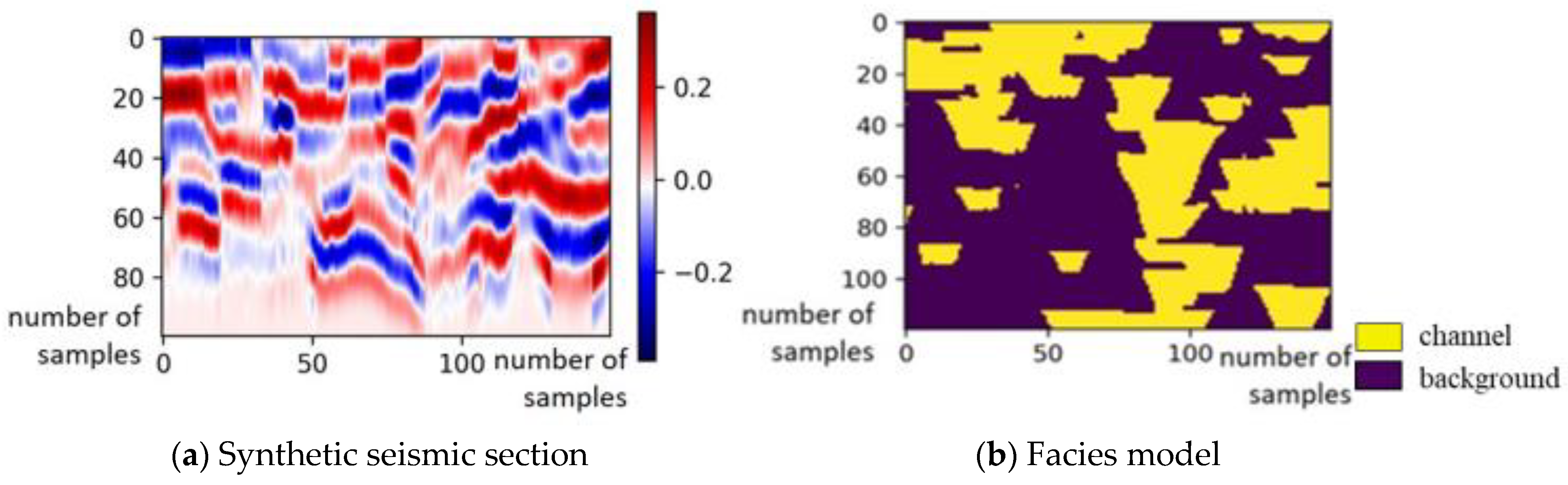
2.1.1. The Synthetic Dataset

The synthetic dataset that is featured in this study was modeled based on the Stanford VI synthetic model [18]. The dataset is an array of synthetically generated 2D normal-incidence seismic sections. The Stanford VI facies model corresponds to a prograding fluvial channel system. The facies model was populated with petrophysical properties, and based on those properties, forward modeling of post-stack seismic data was performed [18]. The dataset featured 5000 training examples, 500 validations, and 500 testing examples. A single pair of training example and a corresponding label is shown in Figure 1. The numbers shown along axes are the number of samples. The facies model is simulated in depth, and the corresponding seismic data is modeled in time.

2.1.2. The F3 Dataset

The F3 dataset [19] was obtained in the Dutch sector of the North Sea. The exploration target was the Upper Jurassic–Lower Cretaceous strata. The interpretation based on qualities of seismic reflectors was part of the F3 dataset provided by dGB Earth Sciences. These data were interpreted through points partially covering the seismic section. The dataset featured a 3D seismic cube which was used as the input data for models in this work. The inline 339 from the F3 dataset along with interpretation points and description of classes is shown in Figure 2.

The gaps were filled in the existing interpretation of the inline 339 and the crossline 500 was interpreted to perform tests on it. Final interpretation of seismic section is shown in Figure 3.

In the experiments, 85% of examples from the inline 339 were used as a training set and the remaining 15% served as a validation set. The crossline 500 were used as a test set. In Figure 4, a plot is shown that compares distributions of the inline and crossline data (IL339 and XL500) using the multidimensional scaling (MDS) technique [20]. Each point represents a single seismic trace coming from seismic sections being compared in the two-dimensional MDS space. We can see qualitatively that the inline and crossline traces had somewhat different distributions. This plot will be referred to in the following sections.

2.1.3. The RIPED Dataset

Another 3D post-stack real dataset was provided by the Research Institute of Petroleum Exploration and Development, PetroChina (here called the RIPED dataset). The interpretation of seismic data was performed by interpreters from RIPED and used in our experiments. The main feature of the RIPED dataset was channel bodies that can be seen on seismic sections, and especially on stratigraphic slices. Stratigraphic slices used to highlight channels were obtained by flattening the seismic cube in time on the bottom of the stratigraphic zone and extracting seismic data along constant time planes. The interpretation of the horizon used for flattening was also provided by RIPED. The main channel system is represented by channels with N–S orientation, and the additional system is oriented in the NW–SE direction. The facies identified by RIPED interpreters within the zone of interest were underwater distributary channel, estuary dam, sheet sand, and distal bar.

In an attempt to reduce the cost of seismic data labeling, a small amount of seismic data were interpreted. An example of a partially interpreted seismic section is shown in Figure 5. The “background” facies shown in the figure represent any other facies that were not interpreted as either channels or a fault zone. Eight inlines and two crosslines were interpreted similarly. In this setting, points obtained for one of the crosslines were used as a test set, and the remaining points were split into training and validation sets using an 85%/15% ratio.

Additionally, interpretation of stratigraphic slices was performed to form another dataset for training and testing. Two stratigraphic seismic slices were labeled to be used for training, while another slice was chosen as a test set. An interpreted slice extracted at the time −1034 ms is shown in Figure 6. Here, one of the interpreted slices was used as the test set, and the examples from the other two were split with a ratio of 85%/15% to form training and validation sets.

2.2. Architectures

Three convolutional deep neural network models were featured in this study. All three models showed good results when applied to seismic data [13,21,22]; however, they have different numbers of parameters and costs of training. To understand advantages and disadvantages of the architectures when applied to different datasets, three deep learning architectures were compared in this study, and their descriptions are given in this section.

2.2.1. Fully Convolutional 2D Network with Dilated Convolutional Layers

The fully convolutional 2D network with dilated convolutional layers architecture was based on [21]. In [21], the authors employ a 3D model, while in this work we used a 2D version of this model. The network consisted of two parts: the first part was based on ordinary 2D convolutional layers and the second part was built with 2D convolutional layers with a dilation factor [23] that essentially controlled the increase of the field of view of convolutional filters. Each convolutional layer was followed by a batch normalization layer [24] to stabilize the distribution of the output of the preceding layer and a ReLU activation function [25] to introduce nonlinearity. The final activation function was a softmax activation, which is suitable for a multiclass classification task and outputs the probability of each class. Since the model was fully convolutional, the input was 2D and the output was also 2D, so it mapped a seismic section to a segmented section, where each pixel had a value of the class with maximum predicted probability obtained by learning latent representations of the input. A schematic architecture is shown in Figure 7.

A number of the model parameters treated as hyperparameters are shown in

Table 1. Hyperparameters considered during the training.

Parameter	Values
number of convolutional layers	2, 3, 4, 5
number of dilated convolutional layers	2, 3, 4, 5
kernel size	3, 5, 7
number of filters	16, 32
learning rate	0.0005, 0.001
training example size	16, 32, 64
training example overlap	30, 50, 70, 80
batch size	4, 8, 15
max pooling	True, False
telescopic architecture	True, False

.

The number of filters in all convolutional layers was kept constant across the model. If the max pooling parameter was “true”, every other convolutional layer was followed by a max pooling layer with the 2 × 2 kernel, and after dilated convolutional layers there were upconvolutional layers to preserve image size. Telescopic architecture requires decreasing kernel size by two and increasing the number of filters by a factor of two for each convolutional layer (without the dilation factor). Training samples were constructed by extracting rectangular regions of the size equal to the “training example size” parameter value with horizontal and vertical overlaps set by the “training example overlap” value in percent from interpreted seismic sections.

2.2.2. The 3D Convolutional Network

This architecture consisted of 3D convolutional layers with a fully connected head. It was based on the MalenoV tool [26], which was later improved [22], with the resulting architecture shown in Figure 8. The architecture consisted of three convolutional 3D and three fully connected layers with two max pooling layers after the first and the third convolutional layers. The activation functions used were ReLU activations; the final activation was a softmax activation. Batch normalization layers were introduced after fully connected layers. Three-dimensional convolutional layers were designed to work with 3D data, while fully connected layers were capable of processing 1D vectors. Thus, to feed the output of convolutional layers to the first fully connected layer, we flattened it, making it one dimensional. The final prediction was done by a layer consisting of the only node, which, topped with a softmax function, gave the probability of each class, and the class with the maximum probability was given as the output. To leverage spatial awareness of 3D layers, around each of the points used for training or prediction a small 3D subcube of seismic data was taken to form a single training example. Prediction was done for each seismic sample individually in contrast to the model described above. However, to inform the model of each sample’s surroundings, a small 3D volume of data was taken into account.

With the sparse sampling scheme introduced in [22], every other sample was taken into account along each dimension; therefore, the initial size of 65 × 65 × 65 was reduced to 33 × 33 × 33. In this way, the computational time required was reduced significantly with a negligible decrease in accuracy.

2.2.3. The U-Net Architecture

The U-Net architecture [17] was used to tackle the challenge of facies classification. The implementation in Python was adopted from [27] and follows the originally proposed architecture configuration. The architecture was fully convolutional, meaning its input is 2D and output is also 2D. The architecture is shown in Figure 9. It had clear encoder and decoder paths, with the encoder reducing the size of the input and the decoder decompressing the latent space representation back to the original size. Each block except the last block had two convolutional 2D layers followed by an additional layer depending on the paths: for an encoder, it was a max pooling layer, and for a decoder, it was a transpose convolutional 2D layer [28]. Each max pooling layer reduces the size of the input by a factor of two along both height and width dimensions, which reduces the complexity of the following operations while retaining the most important details of the input. Two-dimensional transpose convolution both doubles the input size along two dimensions and calculates the inverse of a convolution operation with a weight matrix, so it also learns some useful features. An additional feature of the U-Net architecture is skip connections that concatenate outputs from encoder path blocks with decoder path outputs, thus mixing low-level and high-level features, which is designed to enhance the result.

Hyperparameter values that were considered are shown in

Table 2. Hyperparameters considered during the training.

Parameter	Values
learning rate	1 × 10−4, 1 × 10−5, 5 × 10−6
network depth (the number of convolutional blocks in both top-down and bottom-up pathways)	3, 5, 6
number of filters in the first convolutional block	16, 32, 64
training example size	64, 128, 256
training example size overlap (in percent, horizontal and vertical)	30, 50, 70
number of epochs	150, 250

.

Rectangular patches of the size equal to a “training example size” value were extracted from initial slices to form a training dataset with overlap equal to a “training example size overlap” value.

2.3. Investigating the Validation–Test Accuracy Gap

During our experiments, we observed a clear and consistent gap between validation and test accuracy, which in some cases was significant. The phenomenon was especially prominent when working with the F3 dataset. This issue is usually caused by the difference in distributions of test data and training data, which is indeed the case in this study. As exhibited in Figure 4, despite a significant overlap between distributions, the test (crossline) and training (inline) data clearly differed from each other.

To confirm that the validation/test accuracy gap is caused by differences in distributions and to better understand how the gap is affected by this difference, the following experiment was performed. In the comparative study, we used an inline to construct the training and validation sets and a crossline to form the test set, which caused the distribution difference. We updated the datasets by exchanging some number of examples coming from inline and crossline to reduce the difference in distributions between them. Instead of using only examples extracted from the inline to form training and validation sets, we substituted some of them with examples extracted from the crossline. The same procedure was applied to the test set: a number of examples from the crossline that were previously used as test data and moved to the training/test set were substituted by the same number of inline examples from those that were no longer used for the training and validation sets. Thus, adding to the training and validation sets, some crossline data and some inline data to the test set, we reduced the difference in validation and test distributions and examined how the results compared to the initial data.

3. Results and Discussion

This section describes the numerical experiments run with different deep learning architectures on the different datasets and discusses their results.

3.1. Experiments with the Fully Convolutional 2D Network with Dilated Convolutional Layers

The architecture was first tested on the synthetic dataset to validate its ability to handle the task. The result of predicting the test samples is shown in Figure 10. The resulting test accuracy was 0.92, which indicates that the architecture was suitable for handling the task.

The first real dataset the architecture was applied to was the F3 dataset. Hyper parameter tuning was performed by Monte Carlo sampling [29] parameters which were uniformly distributed over a set of possible distinct values. Fifty different sets of parameters were drawn to initialize and train 50 architectures. Prediction results varied significantly between different initializations. The most and least accurate results of predicting facies distribution of the crossline 500 are shown in Figure 11. The test accuracy of the most accurate prediction was 0.85, and that of the least accurate prediction was 0.16. Attempts were made to improve the stability of the model by regularizing it (using Dropout layers [30] with different rates and adding max pooling layers), but they did not have a noticeable effect. Lack of stability may indicate that this network does not have enough expressive power, which may be solved by adding layers, increasing the number of weights, or adjusting the architecture in some other ways—essentially, changing the model.

The history of validation loss and accuracy of the prediction with the highest test accuracy is shown in Figure 12. From the graphs, we concluded that the model did not overfit, and the validation accuracy achieved was close to 1.

However, there is a clear gap between the validation accuracy and the test accuracy achieved during the training; the validation accuracy was close to 1, while the highest test accuracy was 0.85. To investigate how validation and test distribution difference affects this gap, the test described in 2.3 was performed.

The experiment was performed three times by exchanging 10%, 20%, and 30% of patches from the crossline with patches from the inline. The MDS plot comparing the distributions of test and training samples after exchanging 30% of samples is shown in Figure 13. The mean Mahalanobis distance [31] between the samples in the test set and the distribution of the training set was reduced from 2.90 for the baseline case (corresponding to the points in Figure 4 to 2.66 for the data after exchanging 30% of samples. The difference was reduced, and training samples became more representative of the test set distribution.

The accuracies obtained over five runs for each scenario are shown in

Table 3. Accuracy values obtained with different balancing of a dataset.

	Baseline	0.1 mix	0.2 mix	0.3 mix
accuracy (best case)	0.847	0.886	0.909	0.938
mean	0.823	0.837	0.886	0.931
std	0.021	0.026	0.012	0.006

. Each column in the table corresponds to a particular number of patches from the crossline and the inline mixed to form a training set and a test set (baseline—no mixing). The number of patches extracted from the crossline and placed in the training set was calculated as a fraction (0.1, 0.2, 0.3) of the total number of patches being extracted from the crossline. The same number of patches was taken from the inline and placed in the test set. It was clearly shown that accuracy increases with an increasing amount of mixed data, which provides evidence validating the initial hypothesis.

Additionally, for the F3 dataset, sensitivity analysis was performed to identify which parameters affect prediction accuracy. The technique used to perform the analysis was distance-based generalized sensitivity analysis (DGSA) [32], and it was based on unsupervised clustering of all the response factors being considered into N classes (three in this case) and calculating L1-norm distance between the prior cumulative distribution function (CDF) and the CDF of each cluster for each parameter. If a confidence interval for a parameter centered around 1 did not overlap with its Pareto bar, the parameter was marked as insensitive, otherwise it was marked as sensitive [32].

The result of the sensitivity analysis is shown in Figure 14. The sensitive parameters (shown as blue bars) are the number of convolutional filters, number of dilated layers, batch size, and window size. Unexpectedly, kernel size and number of convolutional layers were insensitive, even though they had a direct effect on the overall number of parameters of the model. The number of dilated layers is more important than the number of regular layers, which may be one reason that the dilation factor in the convolutional kernel allows it to learn more relevant and descriptive features.

Finally, the experiment was performed on the RIPED dataset. As input interpretation and corresponding labels were sparse, a binary mask was introduced to mask unlabeled pixels to prevent the network from learning from pixels with no real labels. The concept and the code were adapted from [33]. The underlying concept was simply multiplying the output from each convolutional layer by 0 where input pixels do not have labels. Data augmentation (horizontal flipping and addition of Gaussian noise) was utilized to increase the number of examples and make the network more robust.

Again, 50 different hyper parameter sets were formed to run 50 independent training and prediction iterations. Examples of predicting the IL500 are shown in Figure 15. The results were unsatisfactory as there were no hyper parameter sets that resulted in a satisfactory prediction.

As mentioned previously, the most likely reason for these poor results was that the amount of training data was very limited, and only part of the distribution represented in the input data was labeled. In addition, channels on seismic sections are very hard to identify precisely, even for human interpreters.

When trained on stratigraphic slices from the same RIPED dataset, however, the model shows a significantly better performance. Though it did not capture all of the small details, it did produce a comprehensive result, achieving a 0.82 test accuracy. The result is shown in Figure 16.

3.2. Experiments with the 3D Convolutional Network

The tool was applied to the synthetic data to assess its performance. To make a 3D model applicable to 2D data, each 2D line was repeated to form the third dimension. The test accuracy obtained was 0.74, and an example of the prediction result is shown in Figure 17. This result was not very accurate, but it captured key details. Since the data was 2D in nature, the 3D model was restricted in its capabilities, which is why this result was poor compared to the other predictions.

Then, an experiment was performed on the F3 dataset. The goal of the experiment was to find an optimal subcube size, treating it as a hyper parameter, and then relate it to some real geological or spatial characteristics of the data. This would allow for the estimation of the subcube size given a new dataset rather than perform hyper parameter tuning again.

To compare results obtained with different subcube sizes, values from 5 to 61 voxels with a step of four were considered for both horizontal and vertical dimensions. The resulting accuracies varied, but not significantly; almost all of the accuracies were within the 0.75 to 0.9 range. In Figure 18, facies classification of the XL500 is shown for different subcube sizes. Overall, the bigger the input subcube, the smoother the predicted result. If a subcube size is too small, the result becomes very noisy (b). However, if the subcube size is big, the result is smooth, but some details may be lost. The dominating facies tends to spread its influence even further (d).

To make geological sense of the subcube size parameter, an experiment was performed to relate it to the two-point correlation (variogram) ranges obtained from the seismic data. Variogram ranges were estimated from the seismic data as 68 samples in the inline direction, 40 samples in the crossline direction, and four samples in the vertical direction. With a sparse sampling scheme (dropping every other sample), the horizontal subcube size based on the variogram range was 35 × 21; the vertical size was increased to nine samples to avoid a very noisy result. The result is shown in Figure 19. The prediction made with a subcube size based on the variogram ranges was significantly more detailed than the base case, which could be potentially attributed to geological features. The test accuracy obtained with the variogram-sized subcube was 0.785. This shows that the two-point correlation of the data can be a reasonable guide to set the parameter value for the input subcube size.

The next experiment involved using the RIPED dataset. The subcube size, which is the amount of data around each seismic sample taken into consideration, was a hyperparameter, and 15 different sizes were tested. The network was trained for two epochs, and the best result of predicting the IL540 is shown in Figure 20.

In this case, there were no fully labeled examples, so the accuracy was not calculated.

Blobs classified as channels in the central part of the sections corresponded to the actual channels circled on the seismic section, which were identified as channels by interpreters from RIPED. It can be seen from predicted results that the network misinterpreted most in areas where there were no labels and especially in the faulted zone, which was expected. Overall, channels were correctly but imprecisely predicted by the model; however, the majority of channel bodies were the result of the model being confused by artifacts in the faulted zone.

The model was also applied to stratigraphic slices extracted from the RIPED cube. The result is shown in Figure 21, the best test accuracy obtained was 0.80. In the result, the key details were captured, but it lacked precision. One possible explanation for this is the lack of expressive power of the model.

3.3. Experiments with the U-Net Architecture

First, the same exercise of testing the architecture on the synthetic dataset was performed. An extreme case was tested, with only 13 examples for training and two examples for testing. The prediction result is shown in Figure 22. Though not very accurate, the predicted facies distribution patterns still captured the true facies distribution.

When the entire synthetic training dataset was used to train the model, a test accuracy of 0.95 was obtained, which is the best among all three models. The result is shown in Figure 23.

The model was then used to predict facies distribution in the F3 dataset. As there was a single training section available, a patch extraction process was performed to form a training set. The best accuracy obtained was 0.86, and the result is shown in Figure 24. Several factors could have affected the performance negatively: a significant number of classes to learn and lack of data corresponding to each of the classes; overall lack of data for training such a deep model; and the difference in distributions between the inline used for training and the crossline used for testing.

Investigating the validation accuracy graph in Figure 25, the issue described in Section 2.3 can be identified. The model achieved very high validation accuracy but significantly lower test accuracy on the same F3 dataset.

The same experiment was performed by mixing data patches from inline and crossline to balance out the distributions of the training set and the test set, and the results are summarized in

Table 4. Accuracy values obtained with different balanced dataset modifications.

	Baseline	0.1 mix	0.2 mix	0.3 mix
accuracy (best case)	0.858	0.845	0.918	0.946
mean	0.801	0.806	0.876	0.934
std	0.033	0.037	0.036	0.010

(structured in the same way as the Table 3). Again, the trend of test accuracy increasing with an increasing amount of mixed data is observed. This confirms that the distribution shift accounted for at least a significant share of the validation-test accuracy gap. The experiment also highlights the fact that the distribution shift is a major problem when applying machine learning algorithms to seismic data: seismic data is usually spatially heterogeneous; therefore, the distribution of data changed throughout the cube or from inline to crossline seismic sections.

When applied to the RIPED dataset, with sparsely labeled vertical sections as training data, the model did not yield any meaningful results. The model was then applied to stratigraphic slices from the RIPED dataset. Patch extraction and data augmentation by flipping left–right and adding Gaussian noise were utilized.

In Figure 26, examples of predictions made with different hyperparameters are shown. Overall, in the results, all the main features visible in seismic data were captured. The prediction in (d) was more precise and more detailed than the one shown in (c), which was expected given its deeper network with more weights and longer training. The image in (d) also has some details not present in the interpretation itself. The accuracy achieved is 0.847.

Figure 27 shows results from the interpretation of multiple stratigraphic slices, visualized as isosurfaces delineating the channel geobodies. The interpreted volume was 20 ms in the vertical size. In Section 4 the comparison of training times and prediction times for the different architectures is shown. The good performance of the U-Net architectures came at the cost of a much longer training time. However, once trained, its predictions were faster than the other architectures. The geobody interpretation shown in Figure 27 was obtained in less than a minute.

4. Conclusions

A comparison of architectures in terms of accuracy values on different datasets was performed; its results are shown in

Table 5. Accuracy values of architectures on different datasets.

	Dilated FCN	3D Conv	U-Net
synthetic	0.92	0.74	0.91
F3	0.83	0.81	0.82
RIPED (slices)	0.8	0.8	0.85

. The performance of the 3D convolutional architecture on the synthetic data, which is 2D in nature, was worse than on the 3D datasets. This, together with the fact that in the synthetic dataset there are 5000 training examples and test data comes from the same distribution as training data, may indicate that the 3D convnet is sensitive to the size and dimensionality of input examples. Fully convolutional architectures showed good performance on all the datasets. The key difference between the dilated FCN and the U-Net was that the former was very sensitive to hyper parameter changes, while the latter was overall robust.

The validation/test accuracy gap highlighted in this study emphasizes the problem that is likely to arise when applying ML models to seismic data. Due to geological heterogeneity, it may be impossible to obtain human-level performance on a part of the seismic cube that a model has not seen, even when a significant amount of training data is available for another part of a cube if there are differences in the distributions of the two parts.

Performance comparison in terms of the prediction time is shown in

Table 6. Performance of architectures used measured with a Tesla V100-PCIE 32GB GPU.

	Dilated FCN	3D Conv	U-Net
training time	729 s (40 ep)	115 s (2 ep)	883.6 s (250 ep)
prediction time (one section)	0.74 s	13 s	0.15 s

. The 3D convolutional model is a robust solution, but its predictions take a long time, as it predicts one voxel at a time. Numerical results showed that the 2-point correlation of the data (variogram range) can be a reasonable guide to set the parameter value for the input subcube size around the prediction voxel. The performance of the fully convolutional dilated architecture was similar to that of the U-Net, but it was much more sensitive to changes in hyperparameters. U-Net showed good results (~0.85 accuracy) when trained on stratigraphic slices, and was overall consistent in its predictions. A universal robust solution working with a small amount of training data and sparsely labeled data is yet to be discovered.

References

1. Thadani, S.G. Reservoir Characterization with Seismic Data Using Pattern Recognition and Spatial Statistics. In Geostatistics Tróia’92; Soares, A., Ed.; Springer: Dordrecht, The Netherlands, 1993; pp. 519–542. [Google Scholar]
2. Wong, P.M.; Jian, F.X.; Taggart, I.J.A. critical comparison of neural networks and discriminant analysis in lithofacies, porosity and permeability predictions. J. Pet. Geol. 1995, 18, 191–206. [Google Scholar] [CrossRef]
3. Caers, J.; Ma, X. Modeling Conditional Distributions of Facies from Seismic Using Neural Nets. Math. Geol. 2002, 34, 143–167. [Google Scholar] [CrossRef]
4. de Matos, M.C.; Osorio, P.L.; Johann, P.R. Unsupervised seismic facies analysis using wavelet transform and self-organizing maps. Geophysics 2007, 72, P9–P21. [Google Scholar] [CrossRef]
5. Chopra, S.; Marfurt, K.J. Seismic facies classification using some unsupervised machine-learning methods. In Proceedings of the SEG International Exposition and Annual Meeting, Anaheim, CA, USA, 14–19 October 2018. [Google Scholar]
6. Lubo-Robles, D.; Marfurt, K. Independent component analysis for reservoir geomorphology and unsupervised seismic facies classification in the Taranaki Basin, New Zealand. Interpretation 2019, 7, SE19–SE42. [Google Scholar] [CrossRef]
7. Bagheri, M.; Riahi, M.A. Support Vector Machine-based Facies Classification Using Seismic Attributes in an Oil Field of Iran. Iran. J. Oil Gas Sci. Technol. 2013, 2, 1–10. [Google Scholar]
8. Li, Y.; Anderson-Sprecher, R. Facies identification from well logs: A comparison of discriminant analysis and naïve Bayes classifier. J. Pet. Sci. Eng. 2006, 53, 149–157. [Google Scholar] [CrossRef]
9. Wrona, T.; Pan, I.; Gawthorpe, R.L.; Fossen, H. Seismic facies analysis using machine learning. Geophysics 2018, 83, O83–O95. [Google Scholar] [CrossRef]
10. Zhao, T.; Jayaram, V.; Roy, A.; Marfurt, K.J. A comparison of classification techniques for seismic facies recognition. Interpretation 2015, 3, SAE29–SAE58. [Google Scholar] [CrossRef]
11. Grana, D.; Azevedo, L.; Liu, M. A comparison of deep machine learning and Monte Carlo methods for facies classification from seismic data. Geophysics 2020, 85, WA41–WA52. [Google Scholar] [CrossRef]
12. Waldeland, A.U.; Solberg, A.H.S.S. Salt Classification Using Deep Learning. In Proceedings of the 79th EAGE Conference and Exhibition, Paris, France, 12–15 June 2017; pp. 1–5. [Google Scholar]
13. Dramsch, J.S.; Lüthje, M. Deep-learning seismic facies on state-of-the-art CNN architectures. In Proceedings of the SEG International Exposition and 88th Annual Meeting, Anaheim, CA, USA, 14–19 October 2018. [Google Scholar]
14. Puzyrev, V.; Elders, C. Unsupervised seismic facies classification using deep convolutional autoencoder. In Proceedings of the EAGE/AAPG Digital Subsurface for Asia Pacific Conference, Kuala Lumpur, Malaysia, 7–10 September 2020; pp. 1–3. [Google Scholar]
15. Long, J.; Shelhamer, E.; Darrell, T. Fully Convolutional Networks for Semantic Segmentation. IEEE Trans. Pattern Anal. Mach. Intell. 2014, 39, 640–651. [Google Scholar]
16. Yu, F.; Koltun, V. Multi-Scale Context Aggregation by Dilated Convolutions. In Proceedings of the International Conference on Learning Representations (ICLR), San Juan, Puerto Rico, 2–4 May 2016. [Google Scholar]
17. Ronneberger, O.; Fischer, P.; Brox, T. U-net: Convolutional networks for biomedical image segmentation. In Proceedings of the MICCAI, Berlin, Heidelberg, 5 October 2015; pp. 234–241. [Google Scholar]
18. Castro, S.A.; Caers, J.; Mukerji, T. The Stanford VI Reservoir; 18th Annual Report; Stanford Center for Reservoir Forecasting, Stanford University: Stanford, CA, USA, 2005. [Google Scholar]
19. Project F3 Demo. Available online: https://terranubis.com/datainfo/F3-Demo-2020 (accessed on 14 June 2021).
20. Kruskal, J.B.; Wish, M. Multidimensional Scaling; Sage University Paper Series on Quantitative Application in the Social Sciences; Sage Publications: Newbury Park, CA, USA, 1978; pp. 7–11. [Google Scholar]
21. Pradhan, A.; Mukerji, T. Seismic Inversion for Reservoir Facies under Geologically Realistic Prior Uncertainty with 3D Convolutional Neural Networks; SEG Technical Program Expanded Abstracts; Society of Exploration Geophysicists: Houston, TX, USA, 2020; pp. 1516–1520. [Google Scholar]
22. Chu, W.; Yang, I. CNN-Based Seismic Facies Classification from 3D Seismic Data. Available online: https://cs230.stanford.edu/projects_spring_2018/reports/8291004.pdf (accessed on 14 June 2021).
23. Yu, F.; Koltun, V. Multi-Scale Context Aggregation by Dilated Convolutions. arXiv 2016, arXiv:1511.07122. [Google Scholar]
24. Ioffe, S.; Szegedy, C. Batch Normalization: Accelerating Deep Network Training by Reducing Internal Covariate Shift. In Proceedings of the 32nd International Conference on Machine Learning, Lille, France, 7–9 July 2015; pp. 448–456. [Google Scholar]
25. Nair, V.; Hinton, G.E. Rectified Linear Units Improve Restricted Boltzmann Machines. In Proceedings of the ICML, Haifa, Israel, 21–24 June 2010. [Google Scholar]
26. MalenoV (MAchine LEarNing of Voxels). Available online: https://github.com/bolgebrygg/MalenoV (accessed on 14 June 2021).
27. Tensorflow U-Net. Available online: https://github.com/jakeret/unet (accessed on 14 June 2021).
28. Zeiler, M.D.; Krishnan, D.; Taylor, G.W.; Fergus, R. Deconvolutional networks. In Proceedings of the IEEE Computer Society Conference on Computer Vision and Pattern Recognition, San Francisco, CA, USA, 13–18 June 2010; pp. 2528–2535. [Google Scholar]
29. Metropolis, N. The Beginning of the Monte Carlo Method. Los Alamos Sci. Spec. Issue 1987, 15, 125–130. [Google Scholar]
30. Srivastava, N.; Hinton, G.; Krizhevsky, A.; Sutskever, I.; Salakhutdinov, R. Dropout: A simple way to prevent neural networks from overfitting. J. Mach. Learn. Res. 2014, 15, 1929–1958. [Google Scholar]
31. Mahalanobis, P.C. On the Generalised Distance in Statistics. Proc. Natl. Inst. Sci. India 1936, 2, 49–55. [Google Scholar]
32. Park, J.; Yang, G.; Satija, A.; Scheidt, C.; Caers, J. DGSA: A Matlab toolbox for distance-based generalized sensitivity analysis of geoscientific computer experiments. Comput. Geosci. 2016, 97, 15–29. [Google Scholar] [CrossRef]
33. Uhrig, J.; Schneide, N.; Schneider, L.; Franke, U.; Brox, T.; Geiger, A. Sparsity Invariant CNNs. In Proceedings of the IEEE International Conference on 3D Vision (3DV), Qingdao, China, 10–12 October 2017. [Google Scholar]
Figure 1. Synthetic seismic section (a) and corresponding facies (b). Note that axes show the number of samples, not physical parameters.
Energies 15 01064 g001
Figure 2. Inline 339 (a), crossline 500 (b), interpretation points for the IL339 that came as a part of the F3 dataset (c). In the legend, the different names represent different characteristics of seismic reflectors. grizzly: chaotic, discontinuous reflections; high_amp_continuous: high amplitude continuous reflections; high_amp_dips: high amplitude dipping reflections; high_amplitude: high amplitude continuous reflections; low_amp_dips: low amplitude dipping reflections; low_amplitude: low amplitude dipping reflections; low_coherency: discontinuous reflections of low coherency; background: other reflections.
Energies 15 01064 g002
Figure 3. Final interpretation of the IL339 (a) and the XL500 (b) used as input data for the algorithms. The unlabeled parts were either labeled as background facies or were not taken into account in the training dataset, depending on the algorithm. In the test dataset, unlabeled samples were ignored.
Energies 15 01064 g003
Figure 4. MDS plot comparing the IL339 with the XL500. Grey dots are traces of the IL339 and red dots are traces of the XL500.
Energies 15 01064 g004
Figure 5. Partial interpretation of the IL365 from the RIPED 3D cube (a) along with the initial seismic section (b). The goal of using this kind of interpretation was to test the limits of the algorithms while reducing labeling costs.
Energies 15 01064 g005
Figure 6. Stratigraphic seismic slice extracted at the time −1034 ms (a) and the corresponding label (b). Interpretation was done by interpreters at RIPED. Though there is uncertainty associated with labels, especially where the faulted zone and channels overlap, the goal of this work was to test the supervised algorithm, so human interpretation uncertainty was not taken into account.
Energies 15 01064 g006
Figure 7. A schematic representation of the fully convolutional 2D network. ReLU activation was used after each block except the last one. The final activation waws softmax. Both input and output are 2D.
Energies 15 01064 g007
Figure 8. The 3D convolutional architecture. Based on [22]. ReLU activation was used after each convolutional and fully connected layer except the last one. The final activation was softmax. The input is 3D and the output is a single value (class index).
Energies 15 01064 g008
Figure 9. The U-Net architecture. Based on [17]. Features encoder and decoder paths and skip connections concatenating their outputs. Both input and output are 2D.
Energies 15 01064 g009
Figure 10. Synthetic seismic section (a), ground truth facies model (b) and predicted result (c). 92% accuracy indicates that the architecture is viable and can be applied to the real datasets.
Energies 15 01064 g010
Figure 11. XL500 (a) along with its interpretation (b), prediction with 0.85 accuracy (c), prediction with 0.16 accuracy (d). Prediction performance of the fully convolutional 2D network varies significantly with slight changes in parameter.
Energies 15 01064 g011
Figure 12. Validation loss and accuracy of the prediction with the highest test accuracy. Validation accuracy gets close to 1, no signs of overfitting.
Energies 15 01064 g012
Figure 13. Distributions of training/test samples after applying the balancing procedure. Grey dots: training examples; red dots: test examples.
Energies 15 01064 g013
Figure 14. Sensitivity analysis of hyperparameters. Parameters are num conv layers: number of convolutional layers; num dil layers: number of dilated convolutional layers; n filters: number of filters; lr: learning rate, window size: training example size; overlap: training example overlap; maxpool: max pooling; telescopic: telescopic architecture. The parameters are described in 0.
Energies 15 01064 g014
Figure 15. Inline 500 (a) and examples of facies predicted for it with different hyperparameters (b,c).
Energies 15 01064 g015
Figure 16. Prediction (b) and an interpreted label (c) obtained with the slice-1029 (a) from the RIPED dataset.
Energies 15 01064 g016
Figure 17. Synthetic seismic section (a), ground truth facies model (b) and predicted result (c). The data is 2D in nature, which does not allow the model to leverage its spatial awareness.
Energies 15 01064 g017
Figure 18. Facies classification of the XL500 (a) with different subcube sizes: 5 × 5 subcube (b), 33 × 33 subcube (c), 61 × 61 subcube (d). The bigger the input subcube the smoother the predicted result.
Energies 15 01064 g018
Figure 19. Facies classification for the XL500 with a variogram range sized subcube (a) and a 33 × 33 × 33 subcube (b). Prediction obtained with a variogram-based subcube has more features and details which could be related to actual geological features.
Energies 15 01064 g019
Figure 20. The IL500 with channel bodies circled (a) and an example of predicted facies (b). Notice misclassified channels along the faulted zone (circled in red), which is most likely caused by channel-like reflection contrast and geometry.
Energies 15 01064 g020
Figure 21. The seismic slice-1029 (a), the predicted slice (b) and the corresponding interpreted label (c). In the prediction, the key details are captured, but it is overall not very accurate.
Energies 15 01064 g021
Figure 22. Synthetic seismic section (a), ground truth facies model (b) and predicted result (c). U-Net was trained on 13 training examples. In the prediction the true facies distribution is captured.
Energies 15 01064 g022
Figure 23. Synthetic seismic section (a), ground truth facies model (b) and predicted result (c). U-Net was trained on the entire training set. The prediction is very close to the true facies model.
Energies 15 01064 g023
Figure 24. The prediction result for the XL500 of the F3 dataset (a) and the interpreted label (b).
Energies 15 01064 g024
Figure 25. Validation loss and accuracy of the prediction with the highest test accuracy.
Energies 15 01064 g025
Figure 26. Seismic slice (a) and its interpretation (b) and examples of prediction obtained with U-Net with different hyperparameter sets (c,d). The prediction in (d) is much more detailed than the one in (c), even some details not present in the manual interpretation were captured.
Energies 15 01064 g026
Figure 27. Examples of geobodies obtained from U-Net predictions.
Energies 15 01064 g027