A New Decision Process for Choosing the Wind Resource Assessment Workflow with the Best Compromise between Accuracy and Costs for a Given Project in Complex Terrain

Abstract

In wind energy, the accuracy of the estimation of the wind resource has an enormous effect on the expected rate of return of a project. For a given project, the wind resource assessor is faced with a difficult choice of a wide range of simulation tools and workflows with varying accuracies (or “skill”) and costs. There is currently no guideline or process available in the industry for helping with the decision of the most “optimal” choice—and this is particularly challenging in mountainous (or “complex”) terrain. In this work, a new decision process for selecting the Wind Resource Assessment (WRA) workflow that would expect to deliver the best compromise between skill and costs for a given wind energy project is developed, with a focus on complex terrain. This involves estimating the expected skill and cost scores using a set of pre-defined weighted parameters. The new process is designed and tested by applying seven different WRA workflows to five different complex terrain sites. The quality of the decision process is then assessed for all the sites by comparing the decision made (i.e., choice of optimal workflow) using the expected skill and cost scores with the decision made using the actual skill and cost scores (obtained by comparing measurements and simulations at a validation location). The results show that the decision process works well, but the accuracy decreases as the site complexity increases. It is therefore concluded that some of the parameter weightings should be dependent on site complexity. On-going work involves collecting more data from a large range of sites, implementing measures to reduce the subjectivity of the process and developing a reliable and robust automated decision tool for the industry.

1. Introduction

1.1. The Choice of Wind Resource Assessment Tools and Workflows

In wind energy, the accuracy of the estimation of the wind resource has an enormous effect on the expected rate of return of a project. Wind Resource Assessments (WRAs) involve a number of steps that are combined together in order to estimate the expected Annual Energy Production (AEP) of a planned project, as well as its associated uncertainty. These steps include wind measurements, wind data processing, correction and analysis, long-term wind resource extrapolation, wind resource vertical extrapolation, wind resource horizontal extrapolation, energy production calculation, estimation of the wake effects and estimation of the losses. Many different international standards and country-specific guidelines exist describing the requirements to make a WRA “bankable”, that is, accepted by investors (e.g., [1]).

For a given project, a choice has to be made between different simulation tools with varying accuracies and costs, and with differing functionalities. For example, the entire wind climate (all wind directions) and the AEP can be calculated automatically with some tools, whereas others have to be extended manually in order to extract this information. Some tools focus just on microscale features, whereas some include mesoscale nesting or forcing. As well as tools developed specifically for the wind energy industry, such as WAsP, WindFarmer and WindSim, generic Computational Fluid Dynamics (CFD) tools such as ANSYS CFX and ANSYS Fluent combined with internally-developed scripts are used. Furthermore, some companies use tools that have been developed internally, such as E-Wind from Enercon [2].

If the choice of model is made incorrectly, either many resources are wasted in needlessly high accuracy simulations, or the rate of return is inaccurate and investors risk losing large amounts of money. Today, this choice is often made based on gut feeling, experience and/or internal organisation recommendations and lessons learned. A decision process or tool would help the wind energy industry make fact-based decisions rather than solely relying on human judgement. This could significantly reduce planning uncertainties and risks.

1.2. Wind Resource Assessment in Complex Terrain

There are several complex weather and wind flow phenomena that pose challenges to measuring and modelling the wind resource correctly. This is especially the case in mountainous terrain, which accounts for approximately 30% of the world’s land surface [3]. Complex wind effects over mountainous terrain include flow separation, sudden wind speed and direction changes and high turbulence, all of which negatively impact wind turbine performance and can be difficult to model. In some cases, these negative effects may be offset by benefits such as katabatic winds and gravity-driven downslope winds in stable atmospheric conditions [4]. As well as this, mountainous terrain can lead to weather conditions such as storms or icing, which are difficult to forecast. Furthermore, mountainous locations are often more difficult and more expensive to develop due to restrictions such as steep slopes, narrow roads or poor infrastructure. For the purpose of this paper, such terrain will be referred to as “complex”, although there is no holistic agreed-upon definition in the community.

Some metrics do exist for the definition of “complex terrain”. The industry-standard linear modelling tool WAsP is said to be applicable reliably for slopes up to 30% [5], because flow separation is likely to occur above this value [6]. The WAsP tool includes a calculation module that quantifies the extent to which the terrain exceeds this requirement, using the Ruggedness Index (RIX), which is defined as the proportion of the surrounding terrain steeper than 30%. The orographic performance indicator $\Delta$RIX is defined as the difference in the values of RIX between the predicted and reference locations. If the reference and predicted locations are equally rugged ($\Delta$RIX = 0%), the prediction errors are relatively small. This method of defining “complex terrain” is used widely in the industry by WAsP users, but is limited to a binary classification (either “complex” or “not complex”). There have been some attempts to assess flow complexity objectively using streamlines and other features, for example, [7], but these methods are computationally demanding or require functionality that is not available in wind energy sector tools.

The performance of different wind models and WRA workflows—in terms of cost as well as accuracy—is highly dependent upon the complexity of the site, because this strongly influences the resulting flow phenomena and weather conditions that are to be simulated. Therefore a decision process requires some sort of site complexity classification. As part of the present work, a new method for classifying site complexity is introduced and tested.

1.3. Assessing the Accuracy of Different Tools

The assessment of tool accuracy is a topic that is relevant to the CFD community in general. In this section, some previous studies on the evaluation of CFD tools are described, followed by some previous studies directly related to wind energy.

1.3.1. Evaluation of CFD Tools

Work on the evaluation of the quality of CFD tools has previously been done in the COST Action 732 [8], with the objective of determining and improving model quality of microscale meteorological models for the prediction of flow and dispersion processes in urban and industrial environments. The work was based on the AIAA guideline for the verification and validation of CFD simulations [9], which consists of a framework containing the three environments: reality, computerised model and conceptual model (which contains all the relevant equations). The phrases “model validation”, “model qualification” and “model verification” refer to the difference between reality and the computerised model, the difference between reality and the conceptual model and to the difference between the conceptual and computerised models, respectively. The COST Action involved defining the following evaluation process: (1) Scientific evaluation process; (2) Verification process; (3) Provision of validation datasets; (4) Model validation process; (5) Operational evaluation process. As part of the model validation process, a range of different metrics were defined, including: correlation coefficient, Fractional Bias, Figure of Merit and Hit Rate. This can be evaluated using a statistical evaluation tool, comparing model predictions with observations (reference states). These metrics can only be used if the number of data points is high enough to allow statistical analysis. For wind energy applications, ten-minute averages are usually sufficient, and therefore these metrics are not necessarily applicable here. However, some of the general ideas have been used to develop the method in this work.

Another relevant project on CFD evaluation was the SMEDIS Project [10], which involved developing a methodology for the scientific evaluation of dense gas dispersion models. A large part of this methodology involved a questionnaire that had to be filled out by the modellers, which asked them questions regarding pre-defined evaluation criteria. These included topics such as the purpose of the model as well as the physical and chemical processes modelled. A similar study involved the development of a guideline for the scientific evaluation CFD studies, focusing on factors such as the domain description and the grid set-up, the input data, the turbulence closure, the equation system and solver applied, the boundary conditions, the initial conditions and the output data, as well as various parameterisations important for microscale modelling [11].

1.3.2. Evaluation of Wind Energy Tools

Several previous studies examine and compare the accuracy of different wind modelling tools, including the Bolund Hill Blind Test [12,13], the Askervain Hill Blind Test [14] and the Perdigão field test [15,16]. However, they are all limited to comparisons of wind speeds for chosen wind directions, or to time periods that are much shorter than those required for WRA. Additionally, the results haven’t been assessed in terms of site complexity, and no attempt has been made to estimate model accuracy in advance to help with the choice of model without having to carry out any simulations in advance.

Due to the large number of separate steps, data types and organisations involved in WRAs, it is challenging to accurately and robustly evaluate the accuracy of different tools or workflows. A key obstacle is the lack of availability and suitability of relevant validation data. The authors are only aware of four substantial previous studies directly related to WRA for wind energy applications:

The first study is the New European Wind Atlas (NEWA) Meso-Micro Challenge for Wind Resource Assessment as part of the IEA Wind Task 31 “Wakebench”, which aimed to determine the applicability range of meso-micro methodologies for WRA within the NEWA validation domain https://iea-wind.org/task31/, accessed on 1 December 2021). It did consider the relationship between tool accuracy and cost; however, no attempt was made to predict these parameters in advance in order to help modellers choose the best tool for a given project. Also as part of IEA Wind Task 31, a Wind Energy Model Evaluation Protocol (WEMEP) has been developed https://wemep.readthedocs.io/en/latest/index.html, accessed on 1 December 2021). WEMEP addresses quality assurance of models being used for research and to drive wind energy applications. This is achieved through a framework to conduct formal verification and validation (V&V) that ultimately determines how model credibility is built upon. It is based on the AIAA guide for the V&V of CFD as described in the previous section.

The second study involves a literature review of the AEP assessment errors in the global wind energy industry as well as a summary of how the wind energy industry quantifies and reduces prediction errors and AEP losses [17]. In this work, a long-term trend indicating a reduction in the over-prediction bias was identified. However, the results were not assessed in terms of site complexity and the details of the individual WRA procedures are limited due to confidentiality issues.

The third study involves the blind comparison of a series of AEP estimations carried out by different participants in the so-called “CREYAP” project (“Comparison of Resource and Energy Yield Assessment Procedures”), run by Ørsted and the Technical University of Denmark. In the most recent exercise, AEP estimations were made for the Walney Extension wind farm (https://windeurope.org/tech2021/creyap-2021/, accessed on 1 December 2021). A summary of the findings from the previous exercises concludes that most of the steps involved in WRA require significant improvement, and the study needs extending for complex terrain effects [18]. These comparisons are highly valuable; however, the details and scientific content are limited due to confidentiality issues.

The fourth study involves recent work by the current authors, which compared the accuracy of simulations using seven different WRA workflows at five different complex sites in terms of wind speed and AEP [19]. The wind speed accuracy was assessed by averaging the absolute difference between simulated and measured wind speeds for each 12 simulated wind direction sectors. The AEP accuracy was assessed by comparing the theoretical gross AEP (obtained from combining wind measurements at a validation location with a theoretical power curve) with the gross AEP obtained from the simulation results. This does not provide a true comparison of the predicted AEP with the actual measured AEP; however, it allows the expected errors in wind speeds to be propagated to errors in AEP and avoids difficulties with obtaining and correcting measurement data from operating wind turbines. It was found that the wind speed accuracies do not correlate well with the AEP accuracies, due to the uncertainties and differences between various AEP calculation methods, as well as the strong dependency of AEP on wind speed magnitude and frequency. It was concluded that it is vital to include the AEP estimation step in any assessment of WRA workflow suitability. This will therefore be done in the present work.

1.4. A Compromise between Accuracy and Cost

In an industrial setting, it is not just the tool or workflow accuracy that contributes to the choice of most suitable tool or workflow, but also the costs—or time—involved with applying it. The overall costs, taking into account computational power as well as the preparation, set-up and post-processing time, also need to be considered. Previous work by the current authors showed that in particular the costs due to the simulation set-up and post-processing effort need to be considered when evaluating the total costs of a WRA process [20]. The authors are not aware of any previous studies with an application to wind energy that study this compromise between workflow accuracy and cost. Therefore, the consideration of accuracy and costs will be a central part of the present work.

This immediately brings up the question of what exactly is meant by the “most suitable” tool or workflow. A schematic representation of a possible variation of workflow accuracy (or “skill”) with cost for any given application is shown in Figure 1, where different workflows are represented by the individual points. For this purpose, it is reasonable to assume that the general trend might look something like this, with the accuracy increasing with increasing costs up to a point above which no significant improvement can be seen. The areas that could be deemed unacceptable by the modeller are marked in red. In these regions, the accuracy is lower than the lowest acceptable values, and the cost is higher than acceptable. The marked region is expected to vary depending on the needs and expectations of the modeller. In terms of cost-effectiveness, the “most suitable” workflow could then be identified as the one with the highest skill score for the lowest cost score within the acceptable region—at the flattening-off part of the curve as marked on the figure. It is recognised that these assumptions may not hold in every possible application, and that the users may prefer to define “most suitable” in a different way, for example by defining the lowest computational time. This topic will be examined further in the present work.

1.5. Decision Support Systems

Wind resource assessors do not have the computational resources or time to thoroughly test and compare a wide range of tools applied to a given project in the manner of the studies described in Section 1.3 above. It is important for wind resource assessors to be in the position to choose the most appropriate model before carrying out any simulations. For this, decision support is required.

Many studies have been carried out on the topic of human judgement and decision-making from a social sciences perspective. In general, studies ranging from the 1970s to as recently as 2020 indicate that simple random weighting schemes or linear models often out-perform human judgement, even by experts, for different applications, e.g., [21,22,23,24,25,26,27]. These models involve simply estimating scores of various pre-defined and pre-weighted assessment criteria and adding these scores up in order to get an overall prediction. For energy applications, decision-making methods are applied for various tasks. For example, for energy systems planning, Multi Criteria Decision Analysis (MCDA) is very common, as described in [28]. Various Decision Support Systems (DSS) have been used for design decision-making. For example, Ref. [29] uses a decision support evolution model using Genetic Algorithm (GA) as the evolution algorithm and CFD as the evaluation mechanism. In another study, the optimal values of the key factors on the performance of a micromixer were obtained using CFD, meta-heuristic algorithms, design of experiment (DOE) and Multi-Criteria Decision Making (MCDM) [30], with the goal of improving the mixing index in micromixers. Multi-Objective Particle Swarm Optimization (MOPSO) was found to offer the best performance.

As well as this, DSS have been identified as a key element required for the successful and efficient creation and application of digital twins, an important driver of further cost reduction in the wind energy industry today. As pointed out in [31], the main challenge of digital twin implementation, besides the software integration, is establishing workflows in such dynamic systems. In digital twin technology there is a lack of a novel, holistic, open and universal approach to objectively perform algorithmic selection and recommend analysis approaches [32]. DSS for wind energy digital twins could include, for instance, the use of Probabilistic Graphical Model (PGMs) to represent digital twin data [33], which can prove to be a powerful abstraction for controlling and planning, as segments of PGM (between two time instances) can be seen as Partially Observable Markov Decision Processes (POMDPs). In line with this sentiment, Ref. [34] showed that solutions of the POMDPs optimisation problem can be a powerful and rigorously proven method in identifying the value of structural health monitoring information and optimal maintenance strategies.

However, due to the very small amount of data available for this application—even for seven tools and five sites, there are only 35 data points involved in the decision-making processes—DSS based on data-driven machine learning models is probably not the most appropriate approach. On-going work involves collecting data from hundreds of publications in order to enrich the knowledge base; however, this task is challenging due to the lack of standardised results. The techniques developed in the social science studies mentioned above are therefore more applicable here. Due to the general indication that even simple models out-perform human judgement, a technique involving the estimation of scores of various pre-defined and pre-weighted assessment criteria will be applied.

1.6. Goal of This Work

The goal of this project is to develop a new decision process based on pre-defined and pre-weighted assessment criteria for choosing the most optimal WRA workflow for a given project in complex terrain. This could be used as a decision tool by wind resource assessors in the future. In order to do this, the new decision process, including the parameter definitions and weightings, was designed and tested using the simulations and measurements from seven different Wind Resource Assessment (WRA) workflows at five different complex terrain sites.

The paper is organised as follows: Section 2 is concerned with the design of the decision process based on previous work, Section 3 describes the test and demonstration of the new decision process on five complex terrain sites, Section 4 contains a discussion of the results and Section 5 the conclusions.

2. Decision Process Design

2.1. Basic Concepts

For the decision process design, the following basic concepts introduced in Section 1 were applied:

• The decision process aims to provide a decision on the choice of optimal WRA workflow(s) for a given site for wind resource assessors;
• It includes a new method for the classification of site complexity;
• It involves an assessment of the expected accuracy AND expected costs of applying a range of possible WRA workflows to a given site;
• It includes an assessment of the AEP accuracy and costs, as well as the wind speed;
• It does not require the user to carry out any simulations in order to assess the site or the workflows;
• The estimation of the accuracy and costs of each workflow involve a simple estimation of the scores of various pre-defined and pre-weighted assessment criteria.

For each site tested, the evaluation of the quality of the process is done by comparing the choice of optimal workflow using the expected skill and cost scores to the choice of optimal workflow using the actual skill and cost scores obtained by comparing simulations to measurements at a validation location.

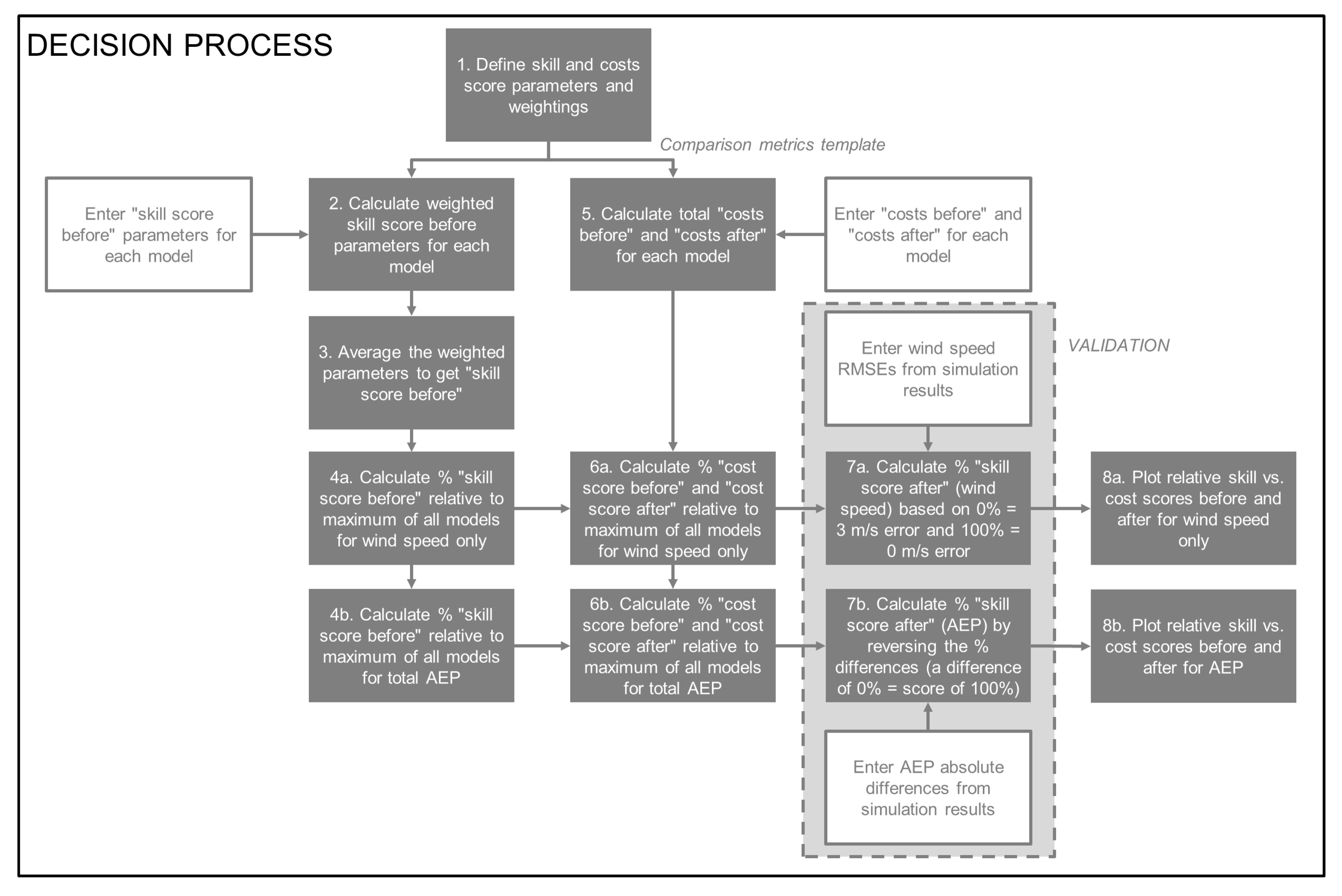
2.2. Description of Decision Process

Based on the basic concepts mentioned above, a decision process was defined as shown in Figure 2. The steps for the validation of the process, marked by the dashed box, will not be part of a future design tool used by the wind resource assessors. This part exists for the validation purposes in the present paper. The individual steps are described in more detail in the next sections.

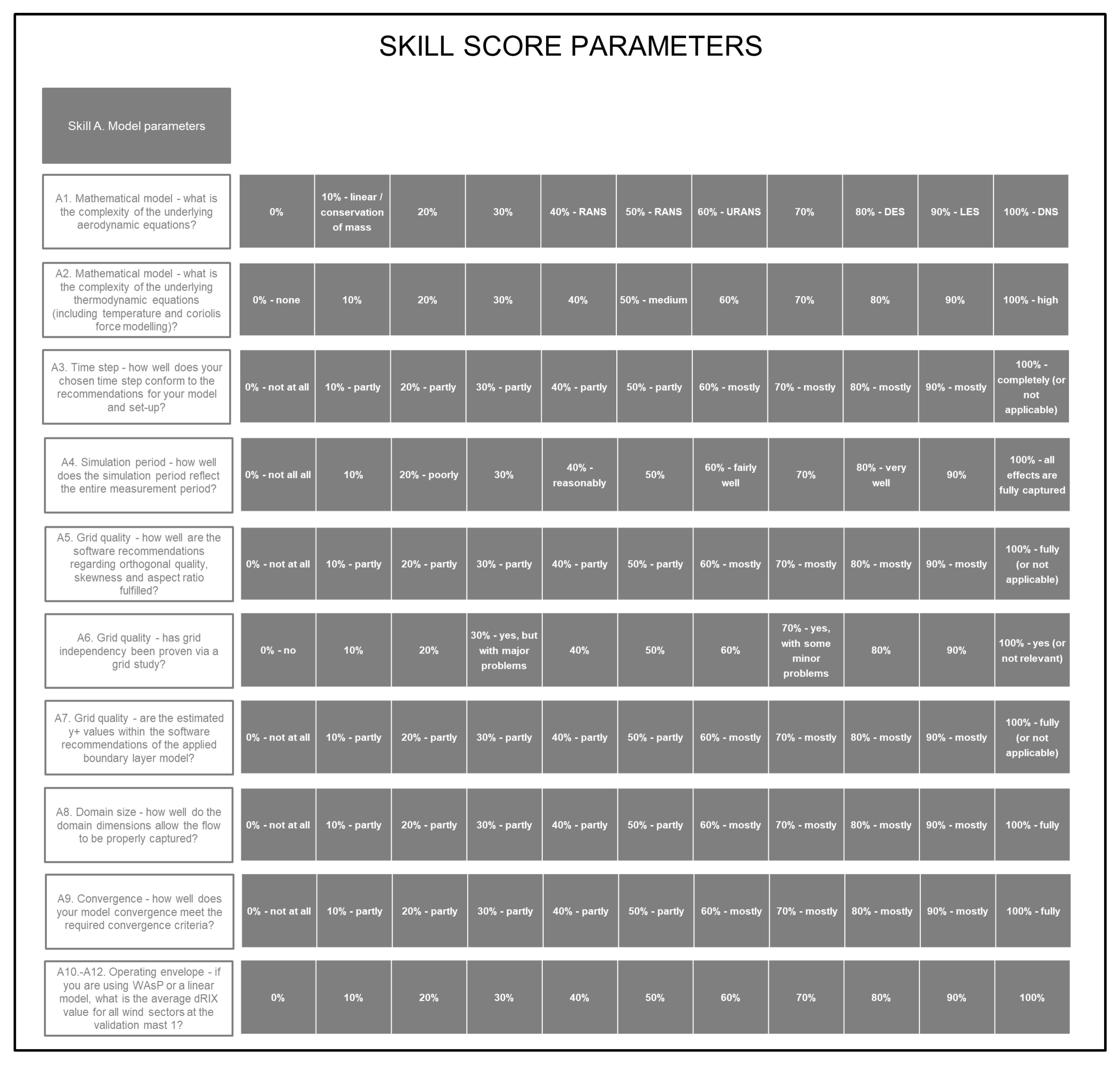
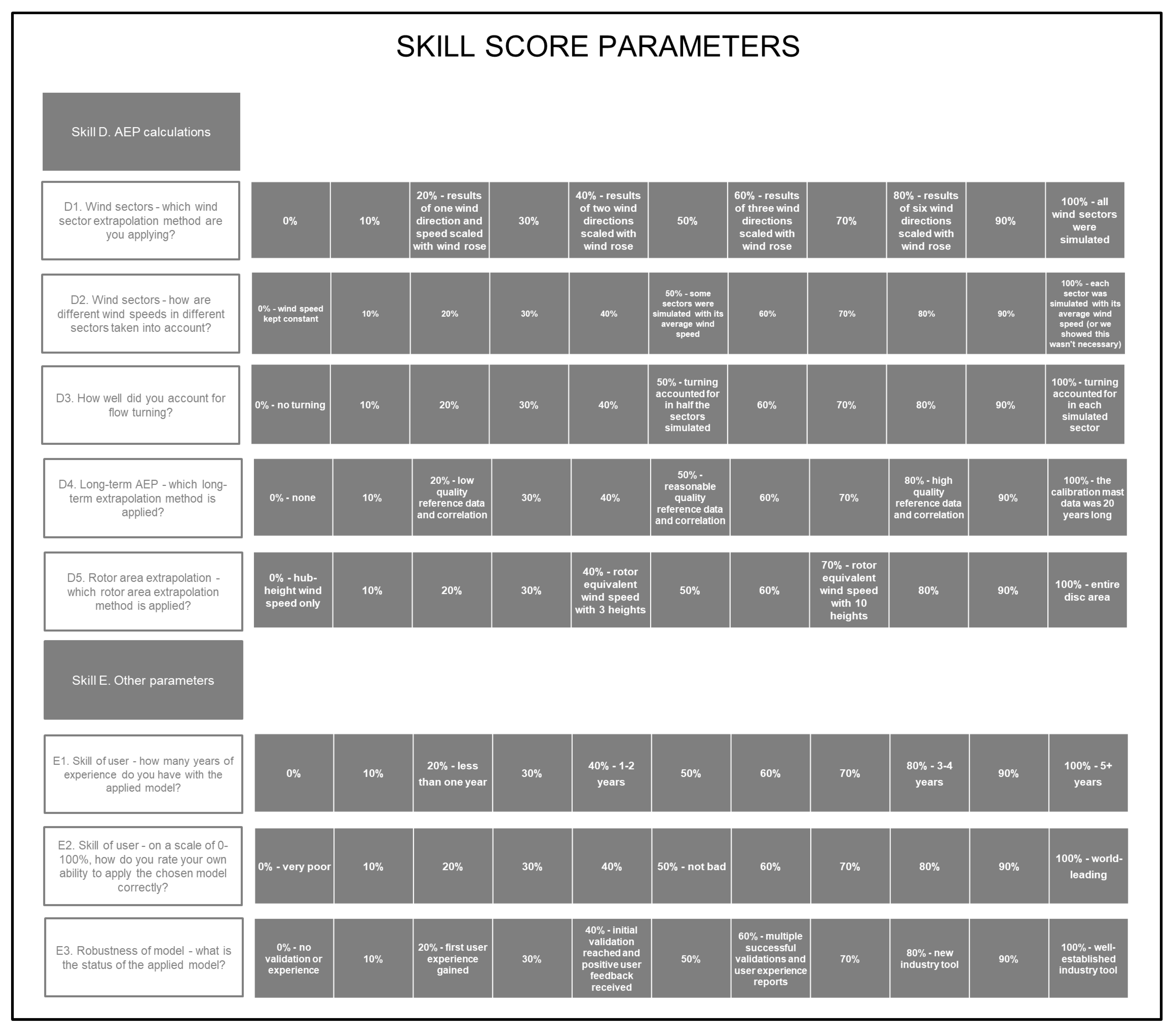
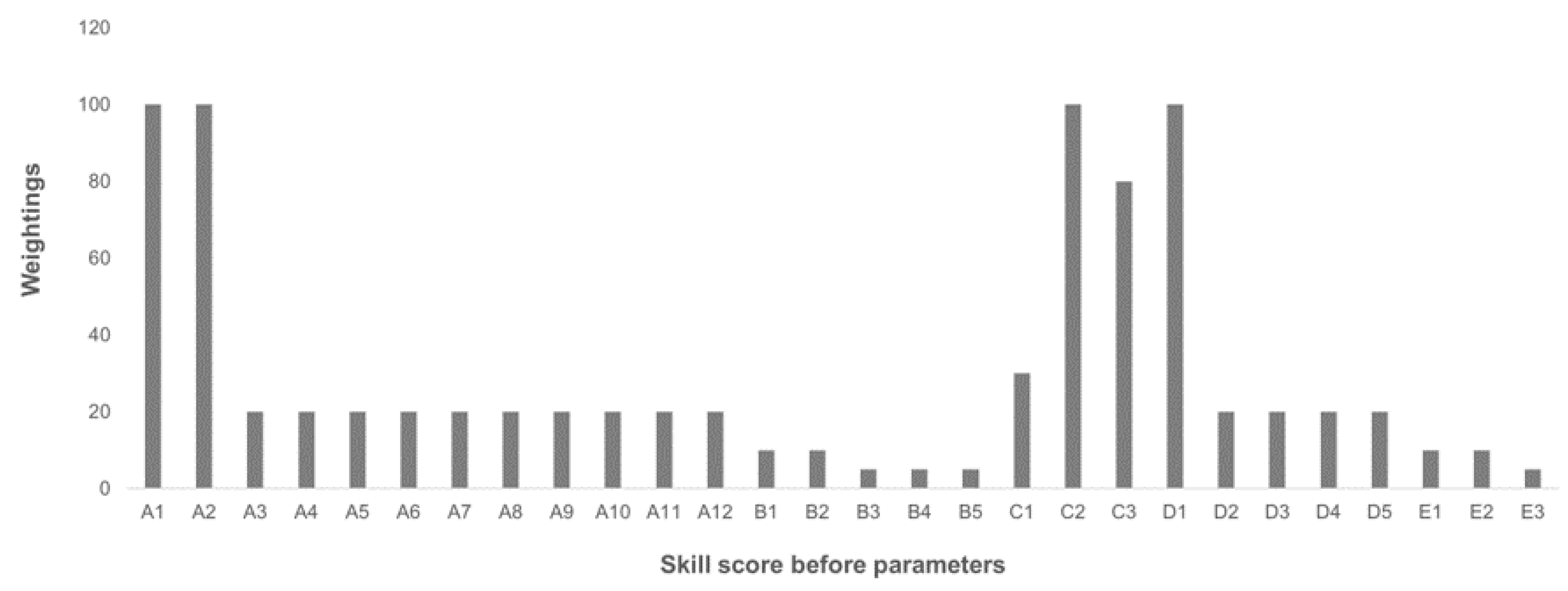
2.2.1. Define Skill and Cost Score Parameters and Weightings

In this step, the skill and cost score parameters and their weightings are first defined. This was done in this work based on initial studies as described in previous work by the authors [16]. The skill and cost score parameters finally decided upon are shown in Figure 3.

The skill score parameters are split into the following five categories: A. Model parameters, related to the wind model set-up such as the fidelity of the aerodynamic and thermal equations, the grid quality and the convergence criteria; B. Input data quality, related to the quality of the data used for model set-up and calibration, including the measurement, terrain and ground cover data; C. Wind model calibration and validation, related to the calibration and validation methods; D. AEP calculations, related to the steps taken to transfer the simulated wind into AEP values, and E. Other parameters, including the skill of the user and the robustness of the model.

Each skill score parameter requires the user to enter a score between 0 and 100 in a web-based questionnaire in which the meaning of the scale of each parameter is described according to Figure A1–Figure A3 in the Appendix A. These scales were designed in order to enable the user to make an educated estimation of the value without having to carry out a complicated calculation.

The weightings were initially defined according to the joint expectations of the researchers taking part in this project. They were improved following simulations at the first simulated site (Site 1) by adjusting them by hand until the sum of the squares of the differences between the expected and actual scores was minimised.

The resulting weightings according to each score listed in Figure 3 are shown in Figure 4. The parameters with the strongest weightings are A1 (complexity of the underlying aerodynamic equations, A2 (complexity of the underlying thermodynamic equations), C2 (wind speed calibration method), C3 (input data method) and D1 (wind sector extrapolation method).

The cost score is estimated by summing the expected software costs, the time to learn and training costs, the simulation set-up effort costs, the simulation run-time costs and the post-processing effort costs. These are entered by the user via a separate web-based questionnaire. In previous work, the total costs, or “Actual Total Costs” (ATCs) were defined by dividing the overall costs into various categories as described in Figure 3 and adding up the totals [20]. The individual costs are obtained as follows:

• Software costs: divide the total license and support costs by the number years of usage, and divide this by the number of projects carried out per year;
• Time to learn and training costs: sum the staff costs for learning the tool and training costs, divide this by the number of projects carried out per year and the estimated number of years of usage;
• Simulation set-up effort costs: record the number of hours needed to set up the simulations, multiply this by the hourly staff rate (for all calculated wind directions);
• Simulation run time costs; record the simulation run-time and the number of cores, and multiply this by the computational cost per core per hour (for all calculated wind directions);
• Post-processing effort costs: record the number of hours needed to post-process the results, multiply this by the hourly staff rate (for all calculated wind directions).

For a fair comparison, the following parameters are normalised over all workflows (value chosen for this work in brackets):

• Number of years of usage of the software (20);
• Number of projects per year (8);
• Staff hourly rate ($100/h);
• Computational cost per core per hour ($0.04/hour/core);
• Processor clock speed (2 GHz).

2.2.2. Calculate Weighted “Skill Score Before” Parameters for Each Model

In this step, the weighted “skill score before” parameters are calculated for each model by multiplying each individual skill score parameter by its weighting.

2.2.3. Average the Weighted Parameters to Get “Skill Score Before”

The weighted parameters are then averaged in order to calculate a “skill score before”.

2.2.4. Calculate Percentage “Skill Score Before” Relative to Maximum of All Models

Using the “skill score before” values estimated for each workflow, a percentage score relative to the maximum of all models for a given project is calculated (a) for wind speed only and (b) for the total AEP. The difference between (a) and (b) is the inclusion of the category D scores (“D. AEP calculations”).

2.2.5. Calculate Total “Costs Before” and “Costs After” for Each Model

Both the total costs before and after are calculated using the results of the separate cost estimations made in the web-based questionnaire mentioned in Section 2.2.1. For the “costs before”, cost estimations are made before carrying out any simulations. For the “costs after”, the actual costs are calculated. The main differences between these two values arise because of incorrect estimations of computational time and of pre- and post-processing effort.

2.2.6. Calculate Percentage “Cost Score Before” and “Cost Score After” Relative to Maximum of All Models

As for the skill scores, a percentage score relative to the maximum of all models for a given project is calculated (a) for wind speed only and (b) for the total AEP. The difference between (a) and (b) is the inclusion of the AEP calculation costs due to additional user effort.

2.2.7. Calculate Percentage “Skill Score After”

The values of percentage “skill score after” for wind speed and total AEP are calculated using the simulation results for each workflow. These values are used in this project for validating the process, but are not part of the final decision process.

For the wind speed, a linear scale is applied, relating a 3 m/s absolute error between simulated and measured wind speed at a validation location to a skill score of 0% and a 0 m/s error to a score of 100%. This scale was chosen based on the actual absolute differences obtained during the project. As relative values are compared, the exact value of this scale is not important.

For the total AEP, the percentage difference between simulated and measured AEP is reversed to relate a difference of 100% to a score of 0% and vice versa. This is because a large difference gives a low skill score, and a small difference a high skill score. As relative values are compared, the exact value of this scale is not important.

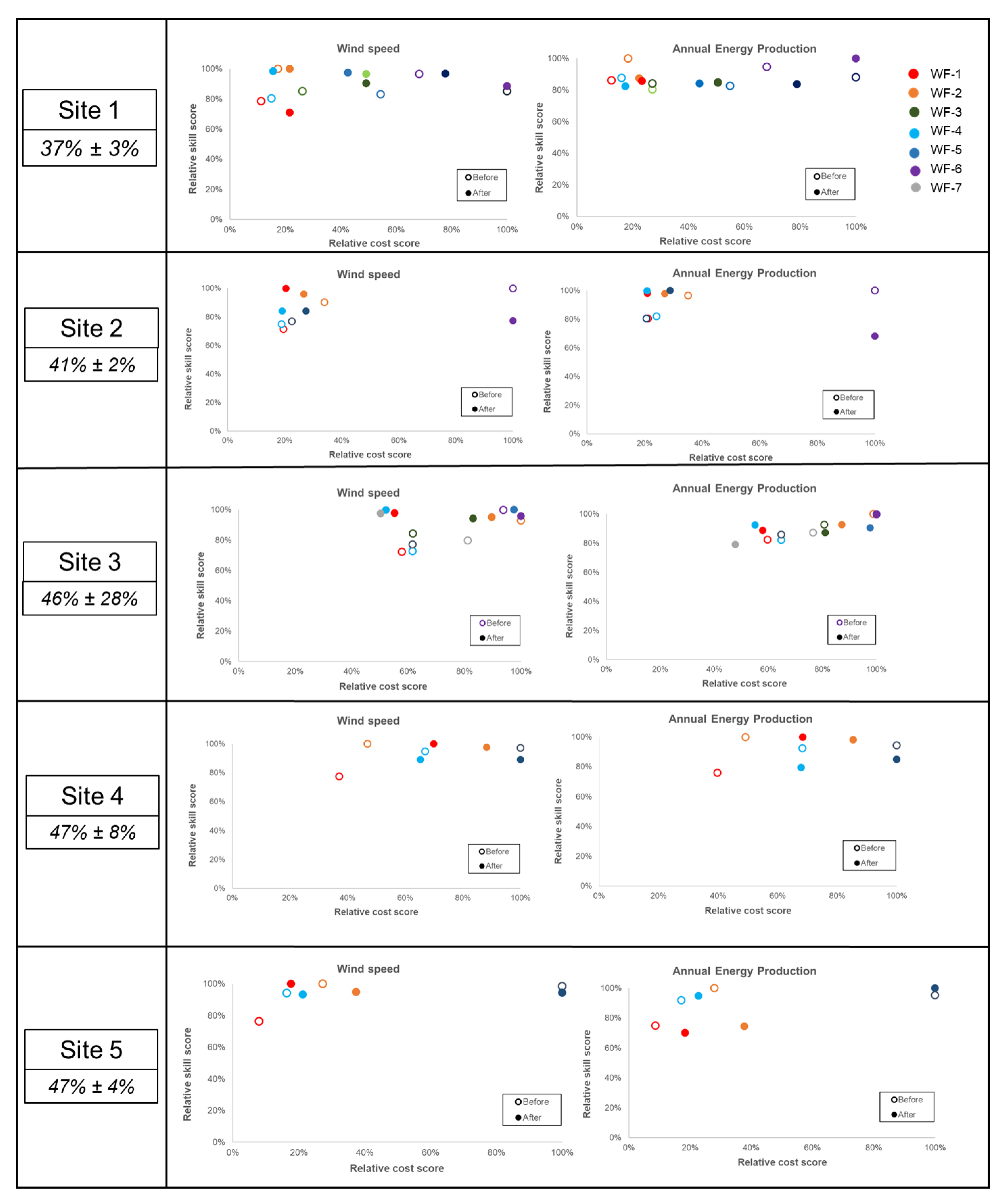
2.2.8. Plot Relative Skill vs. Cost Scores Before and After

In the final step, plots of relative skill vs. cost scores are created both for the “before” scores and the “after” scores, both for wind speed and AEP. As discussed in Section 1.4, these plots can then be used to assess the “most suitable” workflow for a given site. Following discussions with the participants of this study, the definition of “most suitable” has been defined in this work as being the most cost-effective workflow, that is, the workflow highest skill-cost ratio. This is given by the workflow at the apex of the curve, just before it flattens off. However, future work should examine how to deal with other definitions of “most suitable” such as “minimise computational time” or “maximise the skill”.

The process can then be validated by comparing the chosen workflow using the “before” scores and the chosen workflow using the “after” scores. A good match of chosen workflow indicates a successful performance of the decision tool.

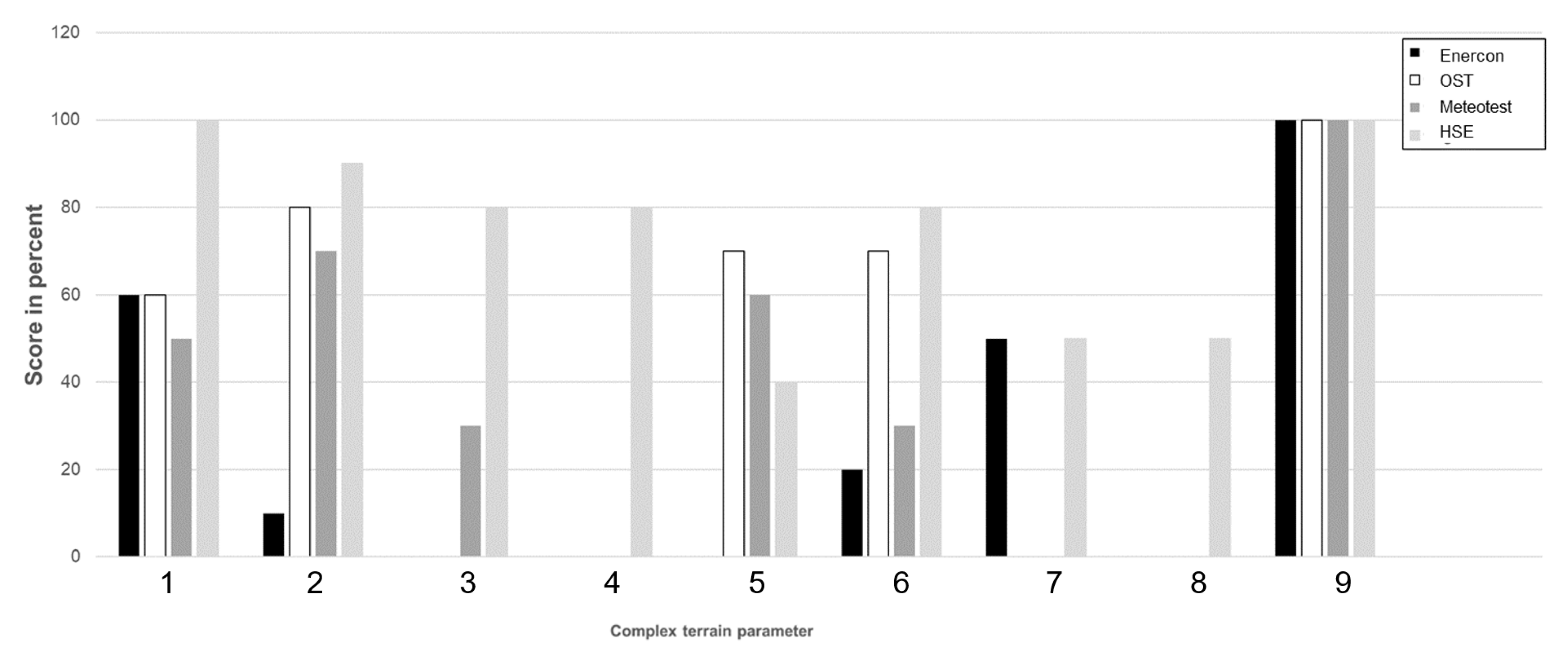
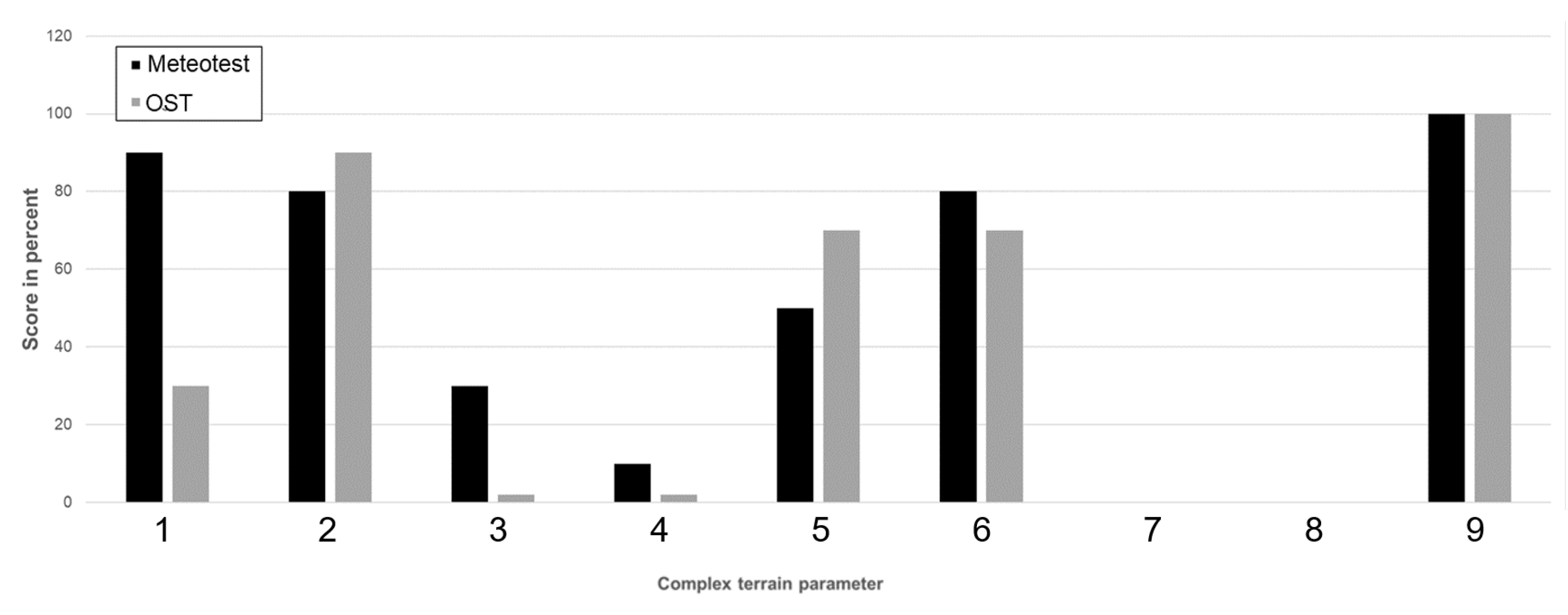
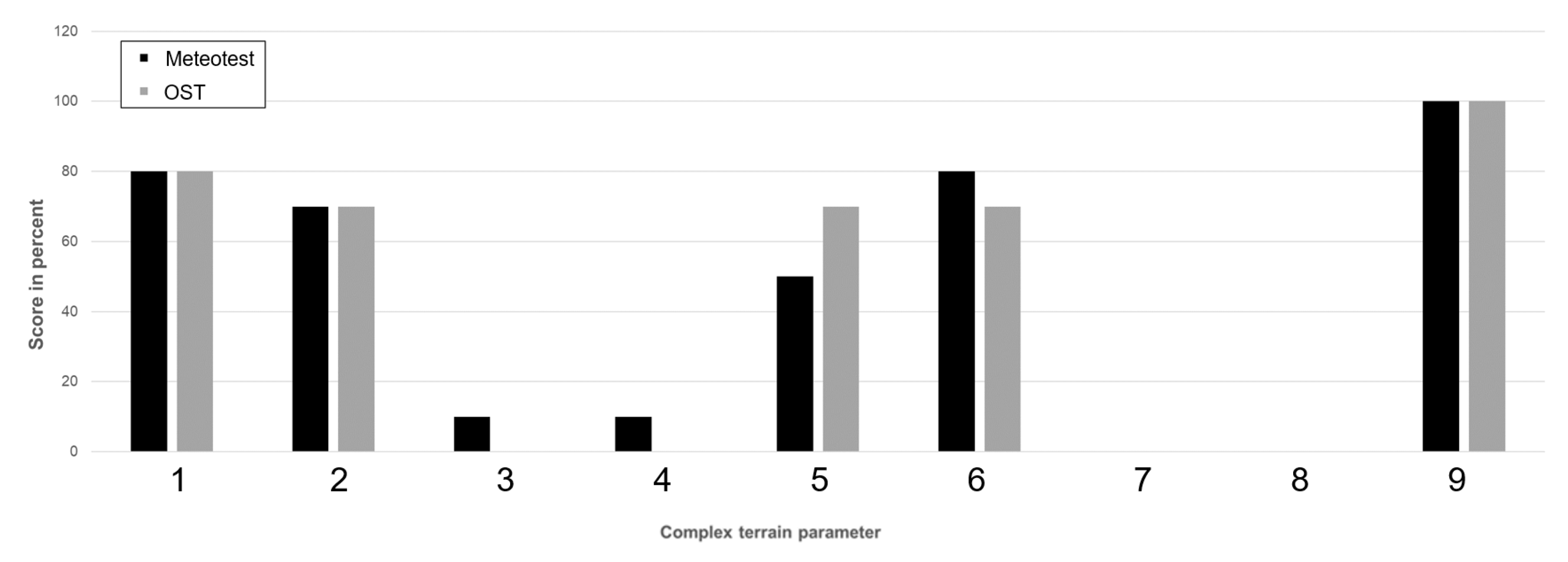
2.3. Classification of Site Complexity

For the classification of site complexity, a set of parameters that users have to rate on a scale of 0 to 100 in a pragmatic way, similar to the method of estimating the skill score parameters described in Section 2.2, were defined. This was based on previous work on terrain classification related to lidar measurements described in more detail in previous work [16]. The parameters were obtained via a web-based questionnaire asking the modeller the following questions:

• General terrain complexity—how steep are the slopes on average?
• General terrain complexity—how many slopes are there?
• Validation mast position—in how many 30° sectors is there a positive slope steeper than 30° less than 250 m away from the validation position in any direction?
• Surface roughness complexity—approximately how many different surface roughness regions are you using?
• Surface roughness—how rough is the surface in general?
• Atmospheric stability—what is the average value of the vertical temperature gradient? (if relevant);
• Atmospheric stability—are low-level jets present?
• Degree of turbulence—what is the approximate Reynolds number, calculated based on the input flow velocity and the distance from the inlet to the calibration met mast?

Each parameter is equally weighted, and a simple average is taken in order to obtain one value that characterises the site complexity.

3. Decision Process Test and Demonstration

In this section, the decision process is tested on one site and demonstrated on four further sites based on simulations from a range of WRA workflows as described in detail in [19]. After the tests on the first site, the weightings of the “skill score before” parameters were adjusted to optimise the results, and then applied to the other four sites.

3.1. Sites and Workflows

Site 1 is a complex terrain, partly-forested site close to Stoetten in southern Germany, whose central feature is a steep incline above 30% and a main wind direction of WNW. Site 2 is an existing wind farm site in Norway surrounded by a terrain of hills, lakes and forests. The wind farm consists of seven Siemens SWT-DD-130 wind turbines with a hub height of 115 m located on a small hill. The two main wind directions are SE and NW. Site 3 is an existing wind farm site in Spain situated in complex terrain. The wind farm consists of 15 Enercon E-40 wind turbines with a hub height of 50 m located at the top of a steep ridge. The two main wind directions are E and NNW. Site 4 is the existing St. Brais wind farm site in Switzerland situated in complex terrain. The wind farm consists of two Enercon E-82 wind turbines with a hub height of 78 m. The main wind direction is NW. Site 5 is a planned site that cannot be described in detail here for confidentiality reasons. More details about the sites can be found in [19].

Seven different WRA workflows based on the wind modelling tools WindPro (labelled “WF-1”), WindSim (“WF-2”), ANSYS CFX (“WF-3”), ANSYS Fluent (RANS: “WF-4”; SBES: “WF-5”), PALM (“WF-6”) and E-Wind (“WF-7”) were applied, as described below:

• WF-1: WindPro: The industry-leading software suite for design and planning of wind farm projects (www.wasp.dk, accessed on 1 December 2021), containing several physical models to describe the wind climate and wind flow over different terrains. For horizontal and vertical extrapolation, WAsP uses a built-in linear flow model, which performs well for flat to moderately complex terrain.
• WF-2: WindSim: An industry software using a Computational Fluid Dynamics (CFD) model based on the PHOENICS code, a 3D Reynolds Averaged Navier Stokes (RANS) solver from the company CHAM.
• WF-3: ANSYS CFX: An all-purpose CFD software. In this work, ANSYS CFX (version 19.2) was applied using an Unsteady RANS approach in combination with the k-$ϵ$ model, with several adaptations including an anelastic formulation using the Boussinesq approximation [35], additional terms in the momentum equation to describe the Coriolis force and a canopy model for forested areas [36].
• WF-4: Fluent RANS: ANSYS Fluent is a commercial CFD tool for modelling the flow in industrial applications and can be set up to solve the RANS equations, as well as for the Large Eddy Simulations (LES) or Detached Eddy Simulations (DES) approach. In this work, Fluent was first set up to solve the RANS equations with the SST k-$\omega$ turbulence model [37].
• WF-5: Fluent SBES: A technique within ANSYS Fluent called “Stress-Blended Eddy Simulation” (SBES) was applied. SBES is a new model that offers improved shielding of RANS boundary layers and a more rapid RANS-LES “transition”, amongst other things. The RANS results were used to initialise SBES, which was performed unsteadily with an adaptive time stepping procedure ensuring CFL <= 1. After an additional unsteady initialisation, the wind speeds were averaged over 10 min.
• WF-6: PALM: The model PALM is based on the non-hydrostatic, filtered, incompressible Navier-Stokes equations in Boussinesq-approximated form (an anelastic approximation is available as an option for simulating deep convection). Furthermore, an additional equation is solved for either the subgrid-scale turbulent kinetic energy using Large-Eddy Simulations (LES) (https://palm.muk.uni-hannover.de/trac/wiki/palm, accessed on 1 December 2021).
• WF-7: E-Wind: E-Wind solves the 3D RANS equations, with a modified k-$ϵ$ turbulence closure. The governing equations are implemented in the open source toolbox OpenFOAM [2].

Further details can be found in [19].

3.2. Test of Decision Process at Site 1

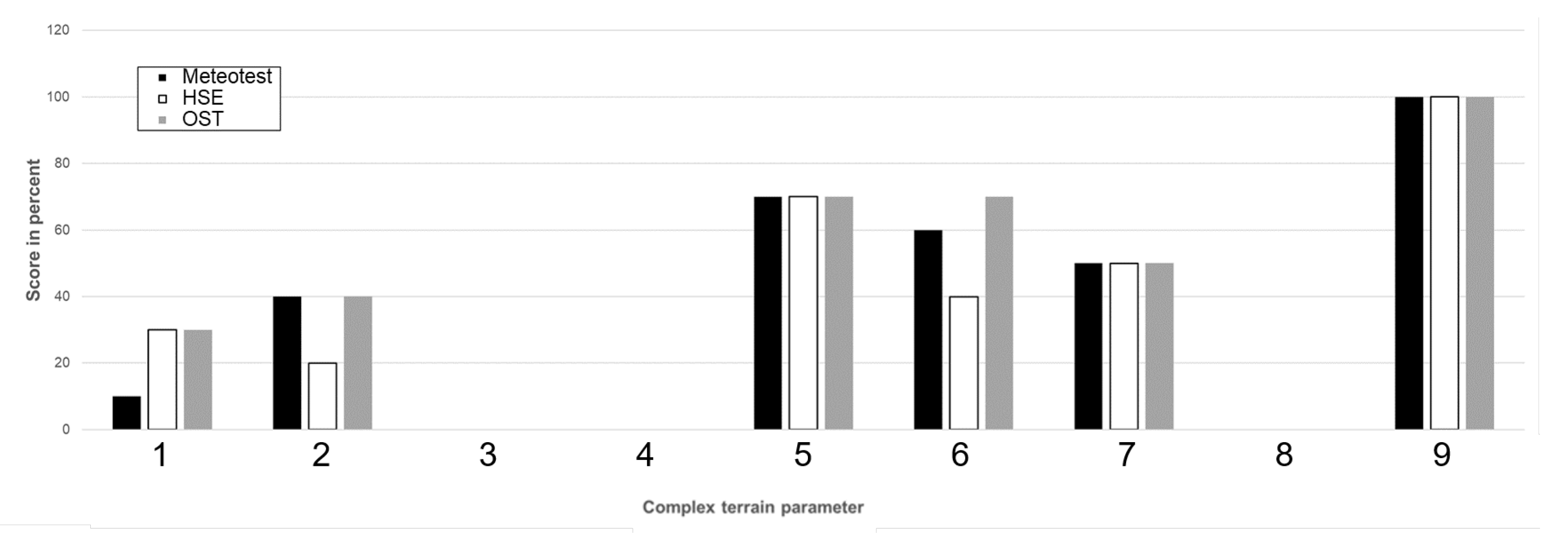
3.2.1. Skill vs. Costs Plots

Detailed simulation results can be found in [19]. The resulting skill vs. costs plots for all sites are shown in Figure 5. For each site, the left-hand plot shows the relative skill vs. cost scores both before and after running the simulations for each model, marked by a coloured circle (before: empty circle; after = filled circle), for the wind speed. The right-hand plots show the results for the AEP results.

For wind speed at Site 1, the “before” results show that WF-1 (WindPro) was predicted to be the least accurate and least expensive model. WF-2 (WindSim) was expected to be slightly more expensive but much more accurate. WF-3 (CFX), WF-4, (Fluent RANS) and WF-5a and 5b (Fluent SBES) were expected to have an accuracy somewhere between the two, but at higher costs. WF-6 (PALM) was expected to be much more expensive but not more accurate. The weightings of the skill score parameters were adjusted by hand until a good match was obtained.

At the end of the day, the most optimal models appear to be WF-2 (WindSim) and WF-4 (Fluent RANS), as they offer a good performance with low costs. A decision tool based on the “skill score before” and “cost score before” would therefore work as expected, choosing WF-2 (WindSim) as the most optimal model. It is important to note that that this analysis does not rate the applicability or accuracy of just the flow models themselves, as many different steps are included in the overall workflow.

The right-hand plot for each site is slightly different due to the conversion of wind speeds in each sector to AEP using the process described in [19]. For Site 1, the skill scores are much closer together, indicating that the wind modelling tool does not have a great effect on the accuracy. This is due to the many steps that are required to carry out a WRA, which all seem to have a relatively large effect on the results. The most interesting feature of this plot is how close the cost and skill scores of WF-1 (WindPro) and WF-2 (WindSim) are to each other, and that WF-4 (Fluent RANS) has the lowest relative cost score. Again, the predictions “before” seem to predict well that WF-1 (WindPro), WF-2 (WindSim) and WF-4 (Fluent RANS) are expected to offer the best compromise, even though the exact scores do not match “before” and “after”.

For this site, the ability of the decision process to successfully predict the most effective workflow for this site has therefore been given a “quality rating” of 8 out of 10 for the wind speed and 8 out of 10 for the AEP. This “quality rating” was estimated by the authors manually from the plots, due to the complexity of an analytical expression to make this judgement.

3.2.2. Site Complexity Characterisation

The results of the answers to the questions presented in Section 2.3 are shown by each research partner organisation for each site in

Table 1. Summary of the answers to the complex terrain questions for each site.

Organisation	Score Site 1	Score Site 2	Score Site 3	Score Site 4	Score Site 5
Meteotest	37	43	43	55	50
HSE	34	43	74	-	43
OST	40	38	42	40	-
Enercon	-	-	27	-	-
Average	37	41	46	47	47
Standard deviation	3	2	28	8	4

. The specific answers to each question for Site 1 are shown in Figure A4 in the Appendix A. This shows that the agreement between the three organisations is fairly good; small differences can be seen in answers to the questions “How many slopes are there?” and “How rough is the surface in general?”. This will be examined further for the other sites.

3.2.3. Summary of Test of Decision Process

For Site 1, the proposed method for estimating and comparing the skill and cost scores for different models for choosing the optimal model for the given application appears to work reasonably well. However, the parameter weightings were adjusted in order to get good results. The other four sites are tested in the next section without adjusting the parameter weightings.

It should also be noted the the differences in skill scores between the wind speeds and the AEP indicate that the different steps contributing to the AEP calculation have a large influence on the results, and that the skill of the wind speed prediction cannot be transferred directly to the AEP. This topic is discussed more in [19].

3.3. Demonstration of Decision Process at Sites 2–5

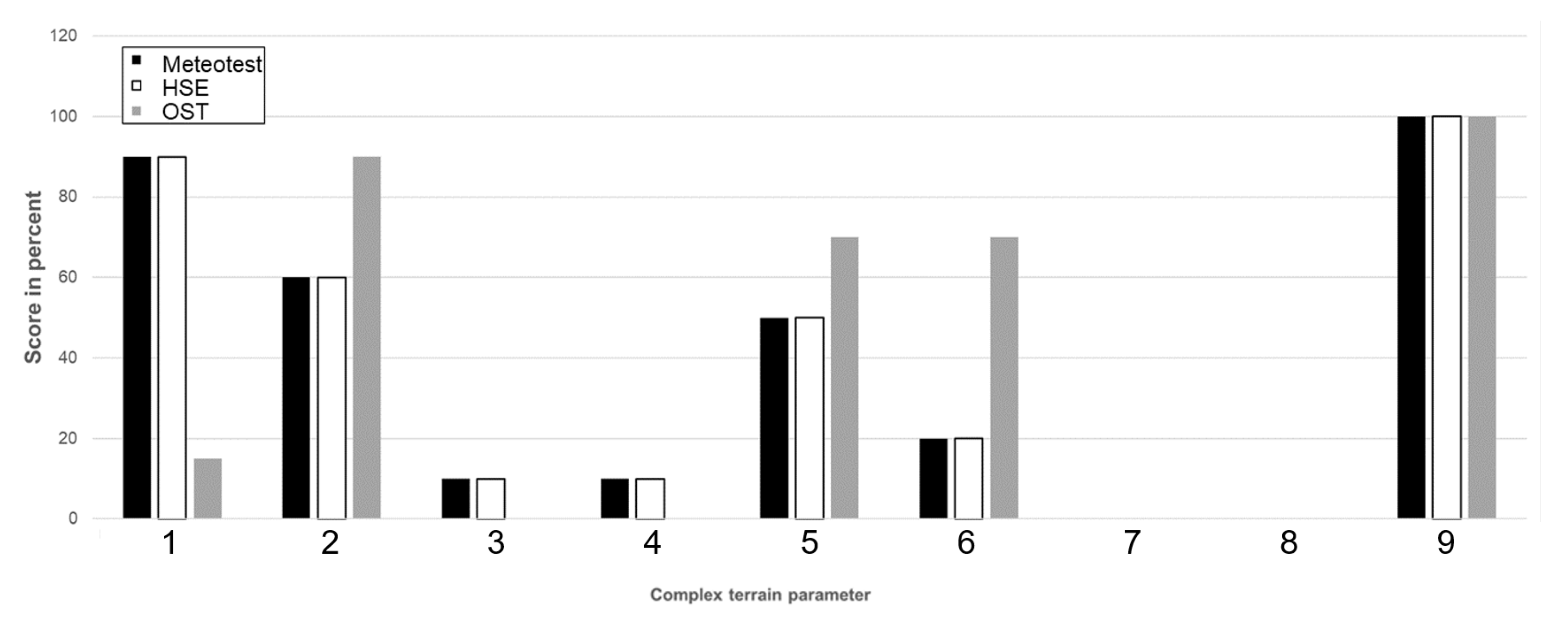
3.3.1. Skill vs. Cost Score Plots

For Site 2, Figure 5 shows that WF-1 (WindPro) was predicted to be the least accurate and least expensive model. WF-2 (WindSim) was expected to be more expensive and more accurate. WF-4 (Fluent RANS) and WF-5 (Fluent SBES) were expected to be somewhere in between these two workflows in terms of skill and cost scores. WF-6 (PALM) was expected to be much more expensive and more accurate. The reality matched these expectations quite well. The main differences were that (a) WF-1 (WindPro) performed much better than expected and (b) WF-6 (PALM) performed much worse than expected. This leads to the conclusion that the skill score parameters do not fully capture the accuracy of the WF-6 (PALM) method. Some resulting improvements to the skill score definitions are suggested in Section 4. The choice of optimal workflow is not entirely clear for the “before” scores, as there is no sudden flattening-off of the curve. The best compromise between cost and skill is probably WF-2 (WindSim). This means that a decision tool based on these predictions would choose WF-2 (WindSim) as the most suitable workflow. However, the most suitable workflow in reality (“after”) is clearly WF-1 (WindPro). This means that the skill score definitions need to be improved, as suggested in Section 4. For AEP, small differences in the predictions (“before”) lead to WF-5a (Fluent RANS) probably being the most optimal workflow for this application. The larger differences in the “after” results, leading to much closer performance of WF-2 (WindSim) and WF-4 and WF-5 (Fluent) compared to WF-1 (WindPro), lead to the most optimal workflow being WF-4 (and WF-1) as well. In this case, the decision tool has worked effectively. The ability of the decision process to successfully predict the most effective workflow for Site 2 has therefore been given a quality rating of 5 out of 10 for the wind speed and 7 out of 10 for the AEP.

For Site 3, Figure 5 shows that WF-1 (WindPro) and WF-4 and WF-5 (Fluent) are expected to have similarly low cost and skill scores, whereas WF-2 (WindSim) is expected to be most expensive and WF-6 (PALM) most accurate. There are several differences that can be observed between the predicted and actual scores. Firstly, all the skill scores are similar, meaning that all the workflows performed very similarly. However, WF-7 (E-Wind) cost less and performed much better than expected. This means that some of the expected inacurracies due to the low resolution of the grid and sub-optimal set-up did not actually translate into a lower actual accuracy. This needs to be investigated further. Some resulting improvements to the skill score definitions are suggested in Section 4. The choice of optimal workflow is not entirely clear for the “before” scores, as there is no sudden flattening-off of the curve. The best compromise between cost and skill is represented by WF-1 (WindPro), WF-4 (Fluent RANS) and WF-5 (Fluent SBES), which all show similar results. A decision tool based on these predictions would choose WF-1 (WindPro) as the most suitable workflow. However, the most suitable workflows in reality (“after”) are clearly WF-7 (E-Wind) and WF-4 (Fluent RANS), although WF-1 (WindPro) comes next. This means that the skill score definitions need to be improved, as suggested in Section 4. For AEP, the predicted most optimal workflows are WF-1 (WindPro), WF-4 (Fluent RANS) and WF-3 (CFX). In reality, the most optimal workflows for this application are either WF-7 (E-Wind), WF-1 (WindPro) or WF-4 (Fluent RANS). Therefore the decision tool has not worked particularly well, with some improvements required. This will be discussed later in Section 4. The ability of the decision process to successfully predict the most effective workflow for this site has therefore been given a quality rating of 3 out of 10 for the wind speed and 3 out of 10 for the AEP.

For Site 4, Figure 5 shows a very nice shaped curve, with WF-2 (WindSim) clearly expected to be the most optimal workflow. Note that this plot looks different to the others because WF-6 (PALM) is not included, which has relatively high costs and therefore causes the relative cost scores of the other workflows to be used. At this site, the most expensive workflow is expected to be WF-5 (Fluent SBES). There are several differences that can be observed between the predicted and actual scores. The shape of the “after” curve is similar to the “before” curve; however WF-1 (WindPro), WF-2 (WindSim) and WF-4 (Fluent RANS) have swapped places. The results indicate that WF-1 (WindPro) would be the optimal workflow for this application, whereas the decision tool predicts WF-2 (WindSim). Therefore further work is required on the optimisation of the skill score predictions. For AEP, the results indicate that the AEP estimation procedure does not have a large influence on the accuracy or on the costs. This is contrary to the other sites, which showed a large variation between the wind speed and AEP charts. This will be discussed further in Section 4. The ability of the decision process to successfully predict the most effective workflow for this site has therefore been given a quality rating of 5 out of 10 for the wind speed and 3 out of 10 for the AEP.

For Site 5, Figure 5 shows that WF-1 (WindPro) was predicted to be the least accurate and least expensive model. WF-2 (WindSim) and WF-4 (Fluent RANS) were both expected to be more expensive and more accurate. WF-5 (Fluent SBES) was expected to be much more expensive and slightly more accurate. The reality matched these expectations quite well. The main differences is that WF-1 (WindPro) performed much better than expected, and cost slightly more. For this site, the skill score parameters captured the behaviour of the workflows quite well. The predicted choice of optimal workflow was WF-2 or WF-4, which are both positioned towards the top left-hand part of the plot. This means that a decision tool based on these predictions would choose WF-2 (WindSim) or WF-4 (Fluent RANS) as the most suitable workflow. The most suitable workflow in reality (“after”) was clearly WF-1 (WindPro), followed by WF-4 (Fluent RANS) and then WF-2 (WindSim). This means that the skill score definitions need to be improved, as suggested in Section 4. For AEP, the predictions (“before”) are very similar to those for the wind speed. The optimal predicted workflow is probably WF-2, or perhaps WF-4, depending on the relative importance of skill and cost to the deciding person. However, as discussed further in [19], there are some differences between the actual (“after”) accuracy of the AEP and the accuracy of the wind speed predictions due to the fact that the RMSE calculation does not “cancel out” over-predictions and under-predictions as the AEP calculation does. This leads to the much higher skill scores for WF-4 (Fluent RANS) and WF-5 (Fluent SBES) compared to WF-1 (WindPro) and WF-2 (WindSim). In reality, therefore, WF-4 turned out to be the optimal compromise between skill and cost. The ability of the decision process to successfully predict the most effective workflow for this site has therefore been given a quality rating of 6 out of 10 for the wind speed and 6 out of 10 for the AEP.

3.3.2. Site Complexity Characterisation

The results for Site 2 in Table 1 and Figure A5 in the Appendix A show that the agreement between the four organisations is not particularly good. There is a maximum deviation from the average value of 50%. The main differences are in the answers to the questions “In how many 30° sectors is there a positive slope steeper than 30° less than 250 m away from the validation position in any direction?”, and “How many slopes are there?” As well as it being difficult to put a number to subjective questions, this shows that the question can easily be misunderstood or interpreted differently between different people. It is therefore clear that this classification method needs to be improved, as discussed further in Section 4.

The results for Site 3 in Table 1 and Figure A6 in the Appendix A show that the agreement between the three organisations is fairly good. The main difference is in the answer to the question “How steep are the slopes on average?”, and small differences can be seen in answers to the questions “How many slopes are there?”, “Approximately how many different surface roughness regions are you using?” and “How rough is the surface in general?” This shows that, although the final result agrees well between the three organisations, it is difficult to put a number to such a subjective question.

The results for Site 4 and Site 5 in Table 1 and Figure A7 in the Appendix A show that it is difficult to assess the results because data is only available from two organisations. In both cases, the variation between the predictions is quite low. In Section 4, we examine how the classification estimations can be used in the decision process in the future.

4. Discussion

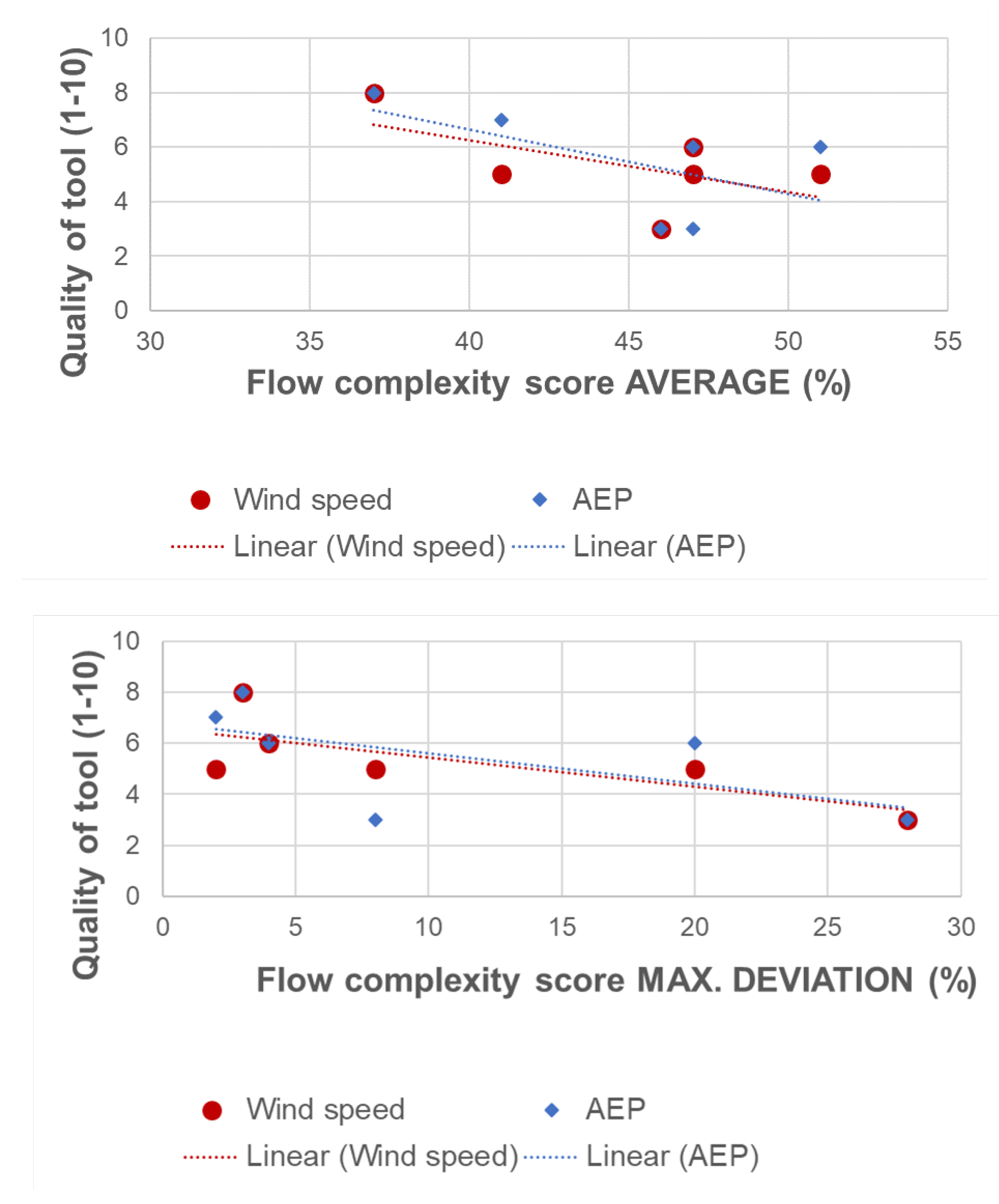
4.1. Dependency of Decision Process Quality on Site Complexity

In the previous section, the quality of the decision process was assessed for each site by comparing the choice of optimal workflow that was made using the predicted skill and cost scores with the choice of optimal workflow that was made using the actual skill and cost scores (calculated by comparing simulations to measurements), both for wind speed and AEP. As well as this, site complexity was quantified for each site by averaging predictions from the different research partners in the project.

The results are summarised in Figure 6, which shows the quality rating of the decision process vs. the complex terrain classification average (upper plot) and maximum deviation (lower plot), both for wind speed (red) and AEP (blue). This shows that the tool quality is negatively correlated with both the site complexity average and the maximum deviation. This indicates that the score estimations need adjusting depending on the complex terrain classification score. This makes sense, as some parameters such as grid quality, aerodynamic equations solved, input data quality and user experience are likely to become more important the more complex the site. This dependence is currently under further investigation.

4.2. Suggested Improvements

In general, the decision process works fairly well for sites with lower complexity (even though the complexity classification scores themselves are associated with some inaccuracies). However, several improvements are required before this can be used in a commercial decision tool, which is the subject of on-going work. The following improvements to the the decision process are suggested in the following sections.

4.2.1. General Method

The process of defining the skill of the model set-up using a web-based questionnaire and then estimating the skill and cost score parameters in a separate questionnaire turned out to be sub-optimal. It requires the user to firstly enter the set-up details, and then to estimate the skill parameters related to these details. This is not only time-consuming and sometimes confusing, but it also leaves a large room for interpretation and subjectivity. The final decision tool will therefore only collect parameters related to the set-up, and then automatically convert this to a skill score in a consistent way.

As well as this, the values entered into the web-based questionnaire were transferred to an Excel template by hand. This template then had to be adjusted for each project. The commercial decision tool will do these steps automatically.

Furthermore, the quantification of the “quality rating” of the decision process could be improved. The rating was estimated by the authors manually from the plots, but more robust methods for obtaining this value are being worked on in connection with the development of the final decision tool.

4.2.2. Skill Score “Before” Estimation

The definition of the scales of the skill score parameters were designed in order to enable the user to make an educated estimation of the value without having to carry out a complicated calculation. However, it is recognised that this is only a first attempt and that improvements are possible, either manually or using regression techniques, for example [38].

Many of the parameters can only be estimated once the simulations have been fully set up. However, the whole point of this method is to be able make an estimation of the most optimal model without carrying out any simulations. Therefore the skill score parameters need to be adjusted so that the user can estimate their values. As well as this, each parameter should have a confidence score associated with it, so that the tool can be applied even if very little information about the set-up is known.

Furthermore, the weightings could be improved using multiple regression techniques rather than informed guesses. Some of them should be dependent upon the terrain complexity classification.

Finally, some of the parameter descriptions were confusing or unclear, and could be improved as listed in more detail in [39].

4.2.3. Cost Scores “Before” and “After”

It turned out to be very difficult to define the Actual Total Costs related to carrying out a WRA project. For example, it was not always clear if an activity was contributing to learning the tool or to the set-up of a particular project. Also, in this project, there were some tasks carried out by one organisation (e.g., the roughness definition), which contributed to their cost scores but were used by the other partners and did not contribute to their cost scores. Furthermore, the staff hourly cost and number of projects per year had to be normalised for a fair comparison. These parameters therefore require further consideration for the final version of the tool.

As well as this, it was very interesting that the set-up effort costs dominated for most of the projects and tools. These costs actually decreased during the project as we became more efficient. This effect skews the results and reduces the accuracy of any comparisons between different sites.

4.2.4. Complex Terrain Classification

Although the new complex terrain classification showed some promise, it was difficult to define questions that the participants could easily answer. Many of the questions were difficult to understand and interpret. Therefore these definitions need to be worked on further.

5. Conclusions

In this work, a new decision process based on pre-defined and pre-weighted assessment criteria for choosing the most optimal Wind Resource Assessment workflow for a given project in complex terrain was developed. The ultimate goal is to use the resulting process in a commercial tool that reduces the uncertainties and risks of Wind Resource Assessment.

The decision process includes a new method for the classification of site complexity. It involves an assessment of the expected accuracy AND expected costs of applying a range of possible workflows to a given site, and includes an assessment of the AEP accuracy and costs, as well as the wind speed. It does not require the user to carry out any simulations in order to assess the site or the workflows. The estimation of the accuracy and costs of each workflow involves a simple estimation of the scores of various pre-defined and pre-weighted assessment criteria. The evaluation of the quality of the process is done by comparing the choice of optimal workflow using the expected skill and cost scores to the choice of optimal workflow using the actual skill and cost scores.

The process was tested on Wind Resource Assessment carried out on five complex terrain sites with seven different workflows. The results showed that the decision process works well, but the accuracy decreases as the site complexity increases. It was therefore concluded that some of the parameter weightings should be dependent on site complexity.

On-going work involves collecting more data from a large range of sites, implementing measures to reduce the subjectivity of the process and developing a reliable and robust automated decision tool for the industry.

References

1. Fördergesellschaft Windenergie. TR 6—Bestimmung von Windpotenzial und Energieerträgen; Fördergesellschaft Windenergie: Berlin, Germany, 2007. [Google Scholar]
2. Alletto, M.; Radi, A.; Adib, J.; Langner, J.; Peralta, C.; Altmikus, A.; Letzel, M. E-Wind: Steady state CFD approach for stratified flows used for site assessment at Enercon. J. Phys. Conf. Ser. 2018, 1037, 072020. [Google Scholar] [CrossRef]
3. Sayre, R.; Frye, C.; Karagulle, D.; Krauer, J.; Breyer, S.; Aniello, P.; Wright, D.J.; Payne, D.; Adler, C.; Warner, H.; et al. A New High-Resolution Map of World Mountains and an Online Tool for Visualizing and Comparing Characterizations of Global Mountain Distributions. Mt. Res. Dev. 2018, 38, 240–249. [Google Scholar] [CrossRef] [Green Version]
4. Parish, T.R.; Cassano, J.J. The Role of Katabatic Winds on the Antarctic Surface Wind Regime. Mon. Weather Rev. 2003, 131, 317–333. [Google Scholar] [CrossRef]
5. Bowen, A.J.; Mortensen, N.G. Exploring the limits of WAsP the wind atlas analysis and application program. In Proceedings of the European Union wind Energy Conference, Göteborg, Sweden, 20–24 May 1996; Zervos, A., Ehmann, H., Helm, P., Stephens, H.S., Eds.; H.S. Stephens & Associates: Bedford, UK, 1996. [Google Scholar]
6. Wood, N. The onset of separation in neutral, turbulent flow over hills. Bound.-Layer Meteorol. 1995, 76, 137–164. [Google Scholar] [CrossRef]
7. Pozo, J.M.; Geers, A.J.; Villa-Uriol, M.C.; Frangi, A.F. Flow complexity in open systems: Interlacing complexity index based on mutual information. J. Fluid Mech. 2017, 825, 704–742. [Google Scholar] [CrossRef]
8. Britter, R.; Baklanov, A. (Eds.) Model Evaluation Guidance and Protocol Document: COST Action 732 Quality Assurance and Improvement of Microscale Meteorological Models; University of Hamburg Meteorological Inst: Hamburg, Germany, 2007. [Google Scholar]
9. AIAA. Guide for the Verification and Validation of Computational Fluid Dynamics Simulations; AIAA: Reston, WV, USA, 1998. [Google Scholar]
10. Daish, N.C.; Britter, R.E.; Linden, P.F.; Jagger, S.F.; Carissimo, B. SMEDIS: Scientific Model Evaluation of Dense Gas Dispersion Models. Int. J. Environ. Pollut. 2000, 14, 39–51. [Google Scholar] [CrossRef]
11. VDI. VDI Guideline 3783, Part 9: Environmental Meteorology—Prognostic Microscale Windfield Models—Evaluation for Flow around Buildings and Obstacles; VDI Guideline 3783; Beuth Verlag GmbH: Berlin, Germany, 2005. [Google Scholar]
12. Bechmann, A.; Sørensen, N.N.; Berg, J.; Mann, J.; Réthoré, P.E. The Bolund Experiment, Part II: Blind Comparison of Microscale Flow Models. Bound.-Layer Meteorol. 2011, 141, 245–271. [Google Scholar] [CrossRef] [Green Version]
13. Berg, J.; Mann, J.; Bechmann, A.; Courtney, M.S.; Jørgensen, H.E. The Bolund Experiment, Part I: Flow Over a Steep, Three-Dimensional Hill. Bound.-Layer Meteorol. 2011, 141, 219–243. [Google Scholar] [CrossRef] [Green Version]
14. Bao, J.; Chow, F.K.; Lundquist, K.A. Large-Eddy Simulation over Complex Terrain Using an Improved Immersed Boundary Method in the Weather Research and Forecasting Model. Mon. Weather Rev. 2018, 146, 2781–2797. [Google Scholar] [CrossRef]
15. Menke, R.; Vasiljević, N.; Mann, J.; Lundquist, J.K. Characterization of flow recirculation zones at the Perdigão site using multi-lidar measurements. Atmos. Chem. Phys. 2019, 19, 2713–2723. [Google Scholar] [CrossRef] [Green Version]
16. Barber, S.; Buehler, M.; Nordborg, H. IEA Wind Task 31: Design of a new comparison metrics simulation challenge for wind resource assessment in complex terrain Stage 1. J. Phys. Conf. Ser. 2020, 1618, 062013. [Google Scholar] [CrossRef]
17. Lee, J.C.Y.; Fields, M.J. An overview of wind-energy-production prediction bias, losses, and uncertainties. Wind. Energy Sci. 2021, 6, 311–365. [Google Scholar] [CrossRef]
18. Mortensen, N.; Nielsen, M.; Ejsing Jørgensen, H. Comparison of Resource and Energy Yield Assessment Procedures 2011–2015: What have we learned and what needs to be done? In Proceedings of the European Wind Energy Association Annual Conference and Exhibition 2015 (EWEA 2015), Paris, France, 17–20 November 2015. [Google Scholar]
19. Barber, S.; Schubiger, A.; Koller, S.; Eggli, D.; Radi, A.; Rumpf, A.; Knaus, H. The wide range of factors contributing to Wind Resource Assessment accuracy in complex terrain. Wind. Energy Sci. 2021. [Google Scholar] [CrossRef]
20. Barber, S.; Schubiger, A.; Koller, S.; Rumpf, A.; Knaus, H.; Nordborg, H. Actual Total Cost reduction of commercial CFD modelling tools for Wind Resource Assessment in complex terrain. J. Phys. Conf. Ser. 2020, 1618, 062012. [Google Scholar] [CrossRef]
21. Yu, M.C.; Kuncel, N.R. Pushing the Limits for Judgmental Consistency: Comparing Random Weighting Schemes with Expert Judgments. Pers. Assess. Decis. 2020, 6, 2. [Google Scholar] [CrossRef]
22. Hogarth, R.; Karelaia, N. Heuristic and linear models of judgment: Matching rules and environments. Psychol. Rev. 2007, 114, 733–758. [Google Scholar] [CrossRef] [Green Version]
23. Grove, W.; Zald, D.; Lebow, B.; Snitz, B.; Nelson, C. Clinical versus mechanical prediction: A meta-analysis. Psychol. Assess. 2000, 12, 19–30. [Google Scholar] [CrossRef]
24. Goldberg, L. Man versus model of man: A rationale, plus some evidence, for a method of improving on clinical inferences. Psychol. Bull. 1970, 73, 422. [Google Scholar] [CrossRef] [Green Version]
25. Dawes, R.; Corrigan, B. Linear models in decision making. Psychol. Bull. 1974, 81, 95–106. [Google Scholar] [CrossRef]
26. Dana, J.; Dawes, R.M. The superiority of simple alternatives to regression for social science predictions. J. Educ. Behav. Stat. 2004, 29, 317–331. [Google Scholar] [CrossRef]
27. Wainer, H. Estimating coefficients in linear models: It don’t make no nevermind. Psychol. Bull. 1976, 83, 213. [Google Scholar] [CrossRef]
28. Kumar, A.; Sah, B.; Singh, A.R.; Deng, Y.; He, X.; Kumar, P.; Bansal, R. A review of multi criteria decision making (MCDM) towards sustainable renewable energy development. Renew. Sustain. Energy Rev. 2017, 69, 596–609. [Google Scholar] [CrossRef]
29. Malkawi, A.M.; Srinivasan, R.S.; Yi, Y.K.; Choudhary, R. Decision support and design evolution: Integrating genetic algorithms, CFD and visualization. Autom. Constr. 2005, 14, 33–44. [Google Scholar] [CrossRef]
30. Nikpour, M.; Mohebbi, A. Optimization of micromixer with different baffle shapes using CFD, DOE, meta-heuristic algorithms and multi-criteria decision making. Chem. Eng. Process.-Process Intensif. 2022, 170, 108713. [Google Scholar] [CrossRef]
31. Wagg, D.J.; Worden, K.; Barthorpe, R.J.; Gardner, P. Digital Twins: State-of-the-Art and Future Directions for Modeling and Simulation in Engineering Dynamics Applications. ASCE-ASME J. Risk Uncert Eng. Syst. Part B Mech. Eng. 2020, 6, 030901. [Google Scholar] [CrossRef]
32. Ribeiro, J.; Carmona, J.; Mısır, M.; Sebag, M. A Recommender System for Process Discovery. In Business Process Management, Proceedings of the International Conference on Business Process Management, Eindhoven, The Netherlands, 7–11 September 2014; Sadiq, S., Soffer, P., Völzer, H., Eds.; Springer International Publishing: Cham, Switzerland, 2014; pp. 67–83. [Google Scholar]
33. Kapteyn, M.G.; Pretorius, J.V.R.; Willcox, K.E. A probabilistic graphical model foundation for enabling predictive digital twins at scale. Nat. Comput. Sci. 2021, 1, 337–347. [Google Scholar] [CrossRef]
34. Andriotis, C.P.; Papakonstantinou, K.G.; Chatzi, E.N. Value of structural health information in partially observable stochastic environments. Struct. Saf. 2021, 93, 102072. [Google Scholar] [CrossRef]
35. Montavon, C. Validation of a non-hydrostatic numerical model to simulate stratified wind fields over complex topography. J. Wind. Eng. Ind. Aerodyn. 1998, 74–76, 273–282. [Google Scholar] [CrossRef]
36. Liu, J.; Chen, J.M.; Black, T.A.; Novak, M.D. E-ϵ modelling of turbulent air flow downwind of a model forest edge. Bound.-Layer Meteorol. 1996, 77, 21–44. [Google Scholar] [CrossRef]
37. Menter, F. Zonal Two Equation k-w Turbulence Models For Aerodynamic Flows. In Proceedings of the 23rd Fluid Dynamics, Plasmadynamics, and Lasers Conference, Orlando, FL, USA, 6–9 July 2012. [Google Scholar]
38. Einhorn, H.J.; Hogarth, R.M. Unit weighting schemes for decision making. Organ. Behav. Hum. Perform. 1975, 13, 171–192. [Google Scholar] [CrossRef]
39. Barber, S.; Schubiger, A.; Koller, S.; Eggli, D.; Rumpf, A.; Knaus, H. A new process for the pragmatic choice of wind models in complex terrainSource—Final report. East. Switz. Univ. Appl. Sci. 2021. Available online: https://drive.switch.ch/index.php/s/DGxWeKQ35nnbPMW (accessed on 1 December 2021).
Figure 1. Schematic representation of the expected skill score against cost score for an example wind energy project.
Energies 15 01110 g001
Figure 2. Overview of the decision process.
Energies 15 01110 g002
Figure 3. List of skill and cost parameters.
Energies 15 01110 g003
Figure 4. Overview of the final weightings of the cost score parameters.
Energies 15 01110 g004
Figure 5. The skill score vs. cost score plots for all sites in this work.
Energies 15 01110 g005
Figure 6. Quality of tool vs. flow complexity score average (top) and standard deviation (bottom) for all five sites (wind speed in red, AEP in blue).
Energies 15 01110 g006