Article

Integral Methodology for the Multiphysics Design of an Automotive Eddy Current Damper

1
Department of Industrial Engineering, University of Rome “Tor Vergata”, 00133 Rome, Italy
2
Department of Applied Science and Technology, Politecnico di Torino, 10129 Torino, Italy
*
Author to whom correspondence should be addressed.
Energies 2022, 15(3), 1147; https://doi.org/10.3390/en15031147
Submission received: 2 December 2021 / Revised: 8 January 2022 / Accepted: 29 January 2022 / Published: 4 February 2022
(This article belongs to the Special Issue Simulation and Optimization of Vehicle Dynamics System)

Abstract

:
The present work reports an integrated (experimental and numerical) methodology that combines the development of a finite element multiphysics model with an experimental strategy to optimally design an eddy current damper for automotive suspensions. The multiphysics model couples the whole set of time-dependent electromagnetic, thermal, mechanical, and fluid–wall interaction (CFD) partial differential equations. The developed FE model was validated against both literature model predictions and in-house experimental data. The electromagnetic model takes into account the magnetic material characteristics of the ferromagnetic material and iron poles. Loss separation and the Jiles–Atherton hysteresis models were invoked to determine the heat generated in the soft iron parts. The computation of the fluid–wall interaction phenomena in the air gap allowed for the prediction of the temperature field across the solid materials, including the magnets. The design of the EC damper addresses the effects of the geometries of the stator and rotor, as they are the most critical geometries for maximizing the functions of an eddy current damper. The magneto-thermal simulations suggested that the heating of the permanent magnets remains within a safe region over the investigated operational frequency range of the eddy current damper.

1. Introduction

The eddy currents in the proposed EC damper originate in a static cylindrical conductor, when it is exposed to oscillating permanent magnets (PMs). The PMs are mounted, together with soft magnetic iron poles (IP), onto a sliding paramagnetic rod, and the latter functions as a magnetic field concentrator. The magnetic field induced by the eddy currents is in the opposite direction to that of the original magnetic field. The former is responsible for a new generated force vector, whose strength is proportional to the velocity of the slider, while its direction has the opposite sign (Lorenz’s law). In our system, an outer steel tube, which encases the conductor and back iron (the magnetic field concentrator), must withstand the imposed dynamic loads.
The described EC system can conveniently be used to design a multitude of other advanced, green, contactless damping or braking devices. Linear and rotary eddy current (EC) dampers are increasingly being used over a wide range of advanced applications with the aim of damping vibrations in vehicles [1,2,3,4,5], controlling vibrations in rotary machines [6], and suppressing and isolating vibrations in levitation systems [7,8], magnetic brakes [9,10], spaces [11] and civil applications [12,13]. The main advantage of an EC damper, over a conventional hydraulic damper, stems from its enhanced dynamics, reliability and the absence of polluting oil. Recent applications claim EC systems can be used for green and efficient (gear-transmission free) regenerators [14].
The structural and functional design of a lightweight EC damper requires an analysis of complex time-dependent and strongly nonlinear electromagnetic, thermal, mechanical, and fluid–wall interaction fields. Non-linearity is involved in the material properties and boundary conditions. The optimal selection of the materials and geometry of the parts is of paramount importance to maximize the performances of EC dampers. In general, mechanical vibration power dissipation is desirable for an EC damper, which inevitably involves a large amount of generated heat and an inherent increase in temperature. This, in turn, may degrade the properties of the PMs, especially when the maximum operating temperature exceeds 80–100 °C. Heat dissipation is dominant in both the conductor tube and the soft magnetic back iron, due to hysteresis and Joule losses.
Various analytical, semi-analytical and FE models have been developed to predict the distribution of the magnetic field. Callaghan et al. [15] analytically calculated a 2D magnetic field, generated by a finite solenoid, in terms of elliptical integrals. Derby et al. [16] solved the magnetic field generated by an ideal solenoid that mimicked axisymmetric PMs. Reich et al. [17] presented a closed-form solution for the magnetic flux density of a hollow cylindrical magnet. MacLatchy et al. [18] analytically computed the retarding force induced by a PM falling inside a conductive tube as a function of the radial magnetic flux density. Jae-Sung et al. [19] analytically solved the axial-symmetric magnetic field generated by a PM sliding along a cylindrical tube. They verified the accuracy of the model by measuring the damping properties at low frequencies. Ebrahimi et al. [1] analytically computed the damping force exerted on a cylindrical piston carrying PMs and IPs while oscillating in a tubular conductor and verified their model both numerically, via FE simulations, and experimentally. They also investigated the heat build-up in their EC damper through a thermal resistance network model. Friedrich et al. [20] proposed a semi-analytical Fourier-based model of a tubular generator for automotive applications. The solution to the magnetic field generated by cylindrical magnets in the tubular generator relied on a coupling method which combines electrical and thermal fields using the Fourier model approach. They validated the model in terms of an FE methodology. Abdo et al. [3] performed more specific EC damper studies for automotive suspension applications using FEM. They compared several configurations and then concluded that a conductive material increases the damping output of the damper.
All the above-mentioned studies involved magnetic field computation, mainly aimed at optimizing the geometry, assuming linear or nonlinear soft iron characteristics. To the best of our knowledge, the effect of soft magnetic material saturation and the hysteresis loops of soft magnetic materials on both damping and power losses were neglected, despite their relevance for the functioning and performances of EC devices.
So far, the only work that has addressed the influence of back iron on damping is that proposed by Pu et al. [5]. They computed the magnetic field by solving an axisymmetric FE model, in combination with a back iron congregation phenomenon The latter has also been analyzed in the present work. The same authors found that magnetic congregation improved the output of an EC damper by concentrating on the magnetic field [5]. The distinctive properties of soft magnetic materials for EC damper applications require high magnetic permeability, magnetic saturation, electrical resistivity and a small hysteresis loop area. The manufacturing of soft-material components for an EC damper inevitably alters their initial hysteresis loop, therefore further increasing the loss area and decreasing saturation [21,22,23]. Pure Fe, low carbon steels as well as Fe-Co, Fe-Si and Fe-Ni alloys are widely used in many electrical machines, including EC dampers, since they can take advantage of their multiple outstanding properties.
The magnetic properties of soft magnetic materials depend on the mechanical and thermal residual stresses that occur after manufacturing. Naumoski et al. [24] investigated the effect of mechanical loading parallel to the magnetic flux on the magnetic properties of non-oriented electrical steels by varying the alloying elements and grain size. They discerned the measured losses into three components [24] using Bertotti’s loss separation model [25]. This model was also applied to evaluate the iron losses in alternating and rotating fields as a function of temperature [26]. The results suggested that losses decreased under small tensile stresses and increased under high ones. However, the losses dramatically rose under compression, especially for low frequencies.
Boglietti et al. [27] presented an alternative approach to separate static losses from dynamic ones. Kowal et al. [28] studied the loss phenomena to predict excess losses using the best fitting of experimental data in the frequency domain. The authors then successfully validated their empirical model in the time domain. Hysteresis losses in ferromagnetic materials were also computed in reference [29] by means of FE, using either an in-line solution or post-processing. The former offers the advantage of including the influence of hysteresis on the magnetic field across the material.
Jiles-Atherton formulated their J-A equation [30] to characterize the hysteresis behavior of soft and hard materials, in terms of magnetization (M). This model is considered the most reliable to date, because of its physical background. The method divides the magnetization function into reversible ( M r e v ) and irreversible ( M i r r ) contributions. The former accounts for the bending of domain walls upon magnetization, whereas the latter accounts for the displacement of pinned domain walls. The five involved parameters ( a ,   α ,   c ,   k   a n d   M s ) should be determined by means of best-fitting procedure over the measured saturated hysteresis characteristics [31]. Although the J-A model is well able to describe the saturated hysteresis loops, it may be inaccurate in accounting for unsaturated (minor) loops. Demenko et al. [32], to overcome this problem, modified the J-A hysteresis model and introduced a tuning parameter to adjust the irreversible contribution of magnetization. Szewczyk et al. [33] then refined the numerical integration strategy to attain the 5 unknown parameters. Currently, more efficient algorithms, such as the Genetic Algorithm [34], Artificial Bee Colony [35] and improved Shuffled Frog-Leaping Algorithm [36], are available to estimate the J-A model parameters.
The refined J-A models not only take into account the manufacturing factors, but also include the temperature and operating frequency factors which, in turn, affect the hysteresis loop of ferromagnetic materials. All such factors of influence tend to decrease M s and/or to increase the area of the loop. For instance, the initial hysteresis loop was altered after plastic deformation in Fe-3 wt.% Si steel sheets [37], as well as after quenching or in a nanocrystalline F e 41.5 C o 41.5 N b 3 C u 1 B 13 alloy [38].
The effects of temperature on the hysteresis loop were analyzed using the J-A model for the case of a non-oriented Fe-Si low alloy steel (using a 2nd order polynomial function) [39] and magnetic field frequency [40].
Thus, unlike the previous FE model analyzed by Pu et al. [5] which accounted for soft magnetic back iron, we herein propose a multifield axisymmetric FE model to comprehensively investigate the effects of back iron on the magnetic field distribution and heat transfer in an automotive EC damper for various operating frequencies. The FE designed model couples the electromagnetic and thermal fields and takes into account the effects of the saturation of soft magnetic materials and the inherent heat dissipation properties for the various operating conditions. To attain an optimal design configuration of the EC damper, a systematic analysis was performed on the component sizes, the material saturation of soft iron, and the hysteresis loop as a function of the damping force.
The methodology behind the model was developed according to the following steps: (a) first, we developed a single magnetic field model; (b) we then tuned and validated the model against literature data; (c) we performed a finer tuning of the geometry parameters (to build an EC damper prototype); (d) we calculated the damping force data from an ad-hoc laboratory test rig as a function of the frequency and stroke amplitude; (e) we then tuned the EC damper model more precisely, on the basis of a successful comparison between the experimental results and FE model predictions, in terms of damping force, in order to obtain an optimal magneto-thermal configuration.
Although the temperature (2nd order polynomial), frequency and residual stresses clearly influenced the hysteresis loop, we did not consider them to prevent numerical convergence problems. These assumptions are justified by the results of our prior investigations, which suggested that the temperature factor may account for a negligible deviation of the hysteresis losses, compared to the overall energy losses [39]. Furthermore, the frequency factor was assumed to be negligible because the typical vibration frequency of the oscillations in automotive suspensions is below 80 Hz [41]. A Polaris Sportsman 800 EFI (QUAD) was chosen as a reference vehicle to design the EC damper. Although a QUAD exhibits different dynamics and stroke characteristics from a passenger car, its Mc-Pherson front suspension provides enough space to insert the instrumentation. The QUAD quarter car model had natural frequencies of 1.84 and 12 Hz, compared with the natural frequencies of a passenger car (0–20 Hz) [41].

2. The Multiphysics Model of the EC Damper

2.1. The Geometry of the EC Damper

Figure 1 shows the essential parts of the EC damper and Table 1 lists the relevant design parameters. The moving piston includes axially magnetized neodymium permanent magnets (PMs) and iron poles (IPs). The choice of IPs, instead of radially magnetized PMs, can be justified by their wider market availability than the latter. Both are bolted onto a paramagnetic inner rod, whose diameter is defined by the designed structural rigidity of the damper. A heat-treated Inconel 718 alloy was selected for the inner rod (surface hardness, HRC 45). The geometrical constraints of the damper were the rod diameter ( D r ) , and the outer ( D o ) and inner ( D i o ) diameters of the encasing pipe (SAE 4340). The geometry and composition of the magnetic piston was chosen so that the performance of the final component was proportional to the number of the magnetic modules. The length of the stator tube was also divided by the same factor. This simplification led to a shorter simulation time.

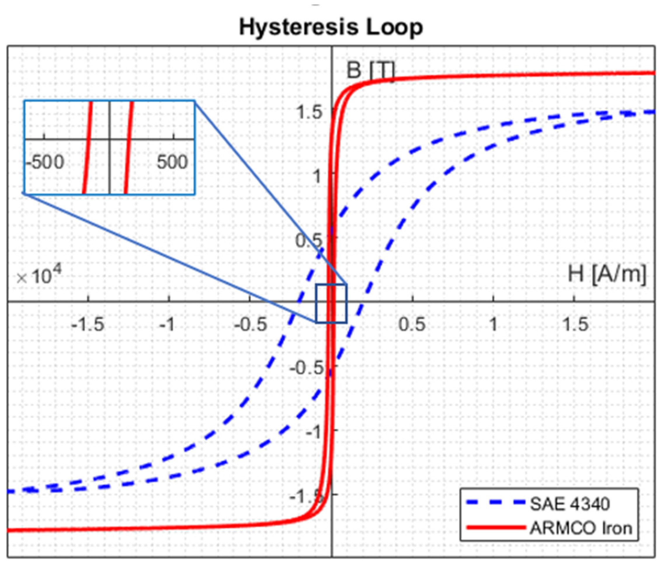
2.2. The Magnetic Model

The magnetic field across the damper is defined in terms of the magnetic vector potential A:
B = 𝛻 × A ,
× H = J ,
where B, H and J are the magnetic flux density, magnetic strength, and surface current density vectors. The current density induced in the cylindrical conductor of volume V generates a magnetic field which is opposite in direction to the external field generated by the moving piston. The latter is responsible for the desired damping force [19]:
F d = ( J × B ) d V ,
As the piston moves along the (axial) z-direction, with a velocity vz, only the radial Br component can exert a damping force, therefore making Bz and Bφ inactive. The damping force for a cylindrical conductor [19] is:
F d = e z ( 2 π σ t c v z r B r 2 ( r , z ) d z ) ,
where t c is the conductor thickness. As it is inspired by a conventional hydraulic damper analysis, the damping coefficient of an eddy current damper can be defined by dividing the given force by the axial velocity vz of the piston:
C = 2 π σ t c r B r 2 ( r , z ) d z ,
As noted in Equations (4) and (5), the radial component of the magnetic flux should be maximized in the conductor to achieve optimal damping. Dimensionless quantities are preferred for both damping coefficient C * = C / C m a x and damping force F * = F d / F m a x , for easy comparison purposes. The damping power is calculated as
P c = F p ν p ,
During normal operation, the EC damper is subjected to Joule losses (across the conducting pipe), electromagnetic losses (in the back iron and steel tube) and friction losses between the sliding parts. Such losses are converted into heat, which increases the damper temperature. As a result, the EC damper functions gradually degrade. The corresponding power loss in the conductor is proportional to the square of the flowing current (I) and to its electrical resistance R(T) which, in turn, depends on the temperature:
P J = R ( T )   I 2 ,
In terms of current density J and electrical resistivity ρ(T), Equation (7) becomes:
P J   = R ( T )   I 2 = ρ ( T )   J 2 V ,
where J = I/A [A/ m 2 ], and A refers to the conductor cross section area and V to the conductor volume.
The magnetic performance of the soft iron material can be accounted for by considering its characteristic hysteresis loop. The classical iron loss model proposed by Bertotti et al. [25] allows the overall losses to be split into two separate contributions, i.e., the static ( P s ) and dynamic ( P d ) ones. The former accounts for the steady-state hysteresis loss ( P h ) of the Weiss domains under a variable magnetic field, while the latter includes the standard eddy current losses, due to the electrical conductivity of the back iron materials ( P e ), and the dynamic losses of the Weiss domains in the presence of a variable magnetic field, called excess losses ( P e x ). Mathematically these losses read:
P = P s + P d   = P h + P e + P e x ,
P e = σ   d 2 12 1 T 0 T ( d B d t 2 ) d t ,
P e x = σ   G   V 0   S 1 T 0 T | d B d t | 3 2 d t ,
where σ is the conductivity, S is the lamination cross sectional area, G is a constant and V 0 refers to the structure dependent internal field.
As per the hysteresis component of the J-A model, the relationship between anhysteretic magnetization M a n and two components was derived from the physics of the magnetization process. This relationship can be expressed as [42]:
M i r r = M a n k δ d M i r r d H e ,
where H e is the effective field, defined as follows:
H e = H + α M ,
d M i r r d H = M a n M i r r k δ α ( M a n M i r r ) ,
M r e v = c ( M a n   M i r r ) ,
d M d H = ( 1   c ) M a n M i r r k δ   α ( M a n M i r r ) + c d M a n d H ,
and δ is a directional parameter which takes on the value of +1 if d H d t > 0 , and −1 otherwise.
In this study, the J-A model parameters for SAE 4340 were taken from reference [43], while the characteristics of the ARMCO pure iron (99.85 wt.% Fe) were calculated from the manufacturer’s data (Figure 2) using the fourth order Runge–Kutta method as a function of the five model parameters [33].
The sum of all the losses was used as the source of the heat in the thermal FE model.

2.3. The Thermal Field Model

Energy dissipation in an EC damper is mainly associated with Joule losses in the conductor as well as with Joule losses and hysteresis losses in the back iron and steel tube. Although high energy dissipation is desired for vibration damping, excessive losses may lead to intense heating of permanent magnets, which in turn leads to their magnetization function and life being reduced to a great extent.
Previous studies addressed the heat transfer problem across the components of the EC damper, using either FEM or semi-empirical models. In general, the former approach provides an accurate evaluation of the overall temperature field in all parts of a device and may also include a reciprocating fluid dynamic analysis. The latter generally invokes empirical convective heat transfer correlations at the cooled walls, which are less computationally costly but also less general.
In an EC damper, only the mean convective heat transfer coefficient that acts over the outer pipe surface can be determined from the empirical knowledge of dimensionless numbers for similar geometrical configurations and heat transfer conditions. The following four dimensionless numbers were introduced: the Nusselt (Nu), Prandtl (Pr), Grashof (Gr) and Rayleigh (Ra) numbers:
N u = hL λ ,
P r = µ c p λ ,
G r = g β ( T s T a ) L 3 ν 2 ,
R a = G r   P r = g β ( T s T a ) L 3 ν α ,
where L, h, λ, u, ν, cp, β, α, Ts and Ta are the characteristic length of the device, the convective heat transfer coefficient, thermal conductivity, the average flow-field velocity, kinematic viscosity, specific heat at constant pressure, the volumetric thermal expansion coefficient, thermal diffusivity, the local surface temperature, and ambient temperature, respectively.
As the EC damper (Figure 1) is arranged vertically, the outer surface of the vertical tube wall was assumed to be cooled by laminar natural convection. The inherent mean heat transfer coefficient was derived using Equation (16) and the following expression [44]:
N u = 0.68 + 0.67 R a 1 6 [ 1 + [ 0.492 P r ] 9 16 ] 4 9 ,
which holds for Ra <   10 9 .
The heat transfer problem in the FE heat transfer model is described as a fully coupled fluid-solid interaction model:
ρ C p T t + ρ C p u · T · ( k T ) = Q ,
under the following assumptions:
  • Air–gas fluid
  • constant temperature at both ends of the stator tube
  • convective heat flux at the outer surface of the external stator tube
Where ρ, C p ,   k ,   u   and   Q are the media density, heat capacity under constant pressure, thermal conductivity for both the solid and fluid domains, and the heat source, respectively. Moreover, the viscosity term μ [ u + ( u ) T ] : u is added to the right-hand side of Equation (22) for fluid media with the viscosity coefficient of μ.
If one wants to apply an analogous Nu number formulation to a reciprocating air flow, they will find that very few literature data are available on the average convective heat transfer coefficients from solid walls to a fluid. Thus, a full FEM heat transfer approach was selected in this study to predict the temperature field across the EC damper components.
The velocity and pressure fields in the air region of the present EC damper model were solved using compressible (Navier–Stokes) momentum and mass conservation laws:
ρ u t + ρ ( u · ) u = · [ p I + μ ( u + ( u ) T ) 2 3 μ ( · u ) I ] + ρ g ,
ρ t + · ( ρ u ) = 0 ,
  • no-slip condition at all the boundaries.
  • compressible and laminar flow
Where ρ, u and μ are the air density, velocity and viscosity, respectively.

2.4. Implementation of the EC Damper Multiphyscis Model

A flow chart of the overall EC damper multifield model, as formulated within the FE Comsol Multiphysics software architecture, is sketched in Figure 3. This chart shows the inter-links between the computational field modules, such as the thermal, electromagnetic, and laminar flow modules, their associated boundary conditions and the moving-mesh technique. It also shows that the magnetic field solution is separated from the solution of the thermal and laminar flow fields, as the thermal losses being converted from the electromagnetic losses are the unidirectional coupling factor (Qh). It should be noted that although full coupling between the electromagnetic and thermal field was considered initially, it was then disabled after verifying that the temperature field had practically no effect on the electromagnetic properties. Thus, the electromagnetic field was the first field to be run and not updated over the complete analysis. The electromagnetic analysis was aimed at achieving two important tasks: (a) finding the optimal dimensions of each part of the EC damper, from the magnetic performance point of view and (b) computing the necessary electromagnetic losses, which were then converted into thermal losses that passed to the thermal-fluid modules.
The piston head was assumed to harmonically displace z ( t ) during operation with a given amplitude and frequency, z ( t ) = a 0 s i n ( 2 π f t ) , starting from a mid-position. The motion of the piston was simulated numerically using an arbitrary Lagrangian-Eulerian moving-mesh formulation [45]. Thus, the moving-mesh strategy applies to all the field analysis.

2.4.1. Implementation of the Magnetic Model

PMs were modeled according to Amperes’ Law, using their magnetic remanence. The magnetic properties of the PMs were taken from the producer’s datasheet (Neodymium 50 M) and had a remanence magnetization of ~1.4 T and a recoil permeability of 1.02. The IPs were modeled, using the initial magnetization curves, based on experimental data provided by the manufacturer. The hysteresis effect was not considered for the iron poles, as they were not subject to an alternating magnetic field. The main electro-thermal properties of the materials are shown in Table 2.
The magnetic field was integrated in time with the moving mesh, using a parallel sparse direct solver (PARDISO), as it provides a faster and more robust solution. The Jacobian matrix was updated at each iteration. The iteration terminated when either a maximum number of 25 iterations or an error between two successive solutions equal to or lower than 10 6   was   reached . The backward differentiation formula (BDF), with an order of accuracy of 1 to 5, was used as the time stepping method. The order of the BDF can be selected automatically during the calculation, depending on the nature of the problem at hand. A high order was used whenever possible, although a lower order is preferred to ensure stability when damping is applied. The total electromagnetic losses in the stator tubes were computed as an important output of the electromagnetic model and converted into cycle average values, using the Fourier transform function. This output was then fed to thermal and fluid flow modules as an internal volumetric heat source.

2.4.2. Implementation of the Thermal Flow Models

The thermal and the laminar flow models were coupled by means of the pressure and velocity fields of the air flow. The required material properties in the thermal model are the thermal conductivities and constant pressure heat capacities of all the involved materials. The material properties in a thermal fluid coupled physics model change with the temperature, and the function of variation was thus included.
The conjugate heat transfer problem was solved across the fluid and solid domains. The fluid domain included heat convection and conduction analyses. Only heat conduction takes place in a solid domain with a volumetric heat source.
Although the laminar compressible Navier–Stokes module accounts for the flow field in the fluid domain, the conjugated heat transfer module accounts for the overall temperature field in the solid and fluid domains. Thus, both fields are directly augmented by the piston sliding from its moving wall.
According to Figure 3, the thermal field analysis is intimately coupled with the fluid flow and fluid–wall interaction fields, while complying with the moving-mesh feature. The multiphysics coupling in Comsol software can be solved using two methods, namely the fully coupled approach and the segregated approach. The former method takes into account all the required couplings at the same time, so that a single large system of equations is built and solved for the complete set of unknowns in one single iteration. The latter method breaks the overall problem down into two or more physics steps, named Segregated Steps. This method is more convenient when the coupled physics becomes excessively memory intensive, even for 2D problems. The segregated algorithm was here combined with the PARDISO direct solver to solve the fluid flow, fluid–wall interaction and thermal field coupling. The problem in our solution strategy was subdivided into two steps. First, the segregated step iterations was initiated to solve the laminar flow (including the fluid–wall interaction) for the velocity and pressure fields. Second, the thermal problem was solved for the temperature field. The cycle-averaged losses were then entered into thermal model as volumetric heat source terms, therefore establishing coupling with the electromagnetic field. In a similar way to the transient analysis of the magnetic field, the BDF was used for time integration, with an order of accuracy of 1 to 5.

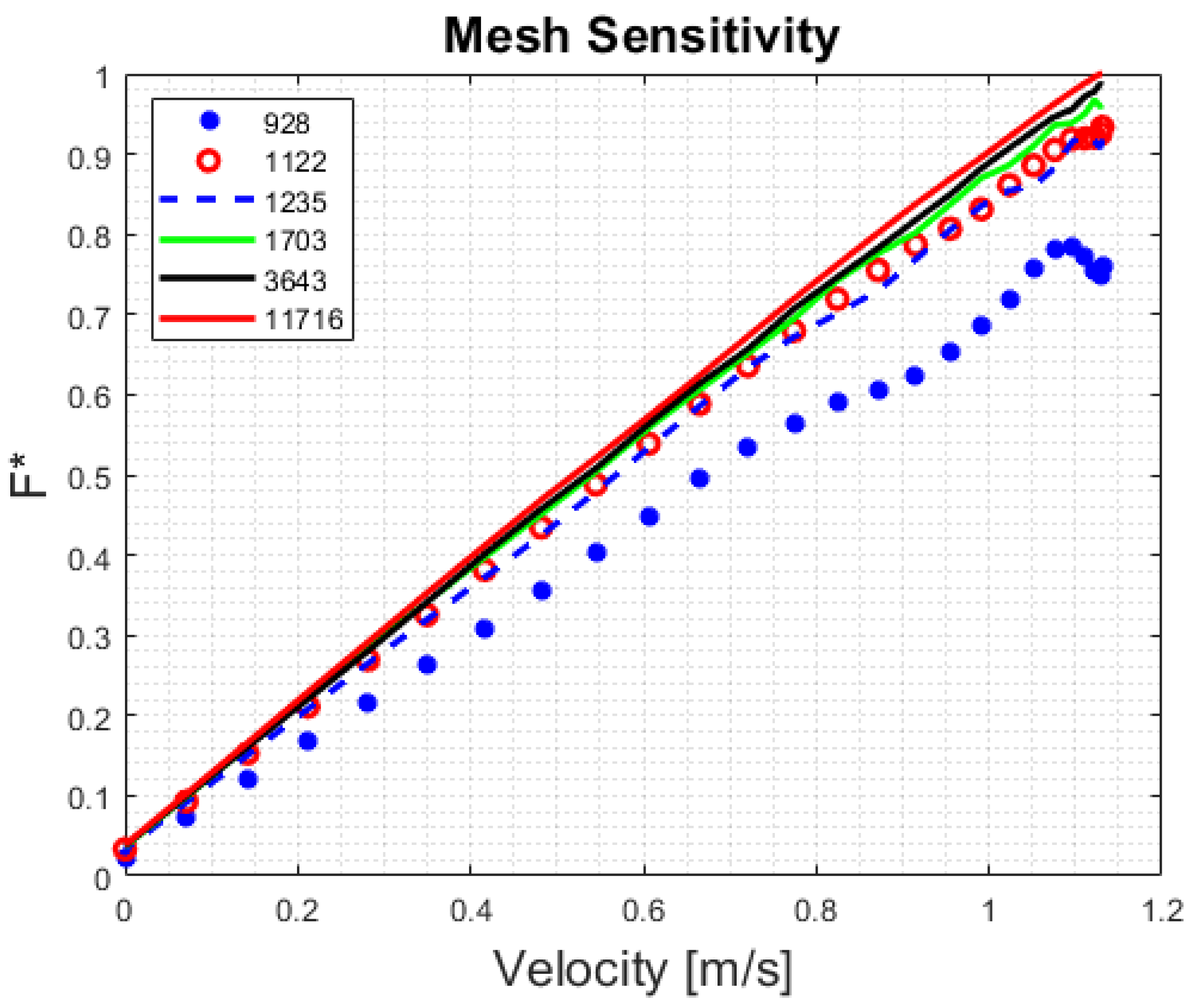
2.5. Mesh Sensitivity Study

The overall geometry of the device was discretized using tetrahedral and brick elements, as shown in Table 3. A Mesh sensitivity procedure was not performed for the temperature field, since, after prior simulation tests, even considering a temperature peak of 80 °C in the domain, which, although crucial for degrading the PM, did not lead to any significant improvement in the overall solution. On the other hand, the conducted tests showed that the mesh size had a much more important effect on the computation of the magnetic field, and it was thus considered for the detailed mesh sensitivity analysis.
A mesh sensitivity study was conducted over the damping force to assess the computational time and model accuracy. The optimal element density was thus determined. Figure 4 reveals that as the mesh became more resolved, the solution became smoother and more detailed. Finally, only 3643 mesh elements were sufficient for solution convergence, within a reasonable simulation time.

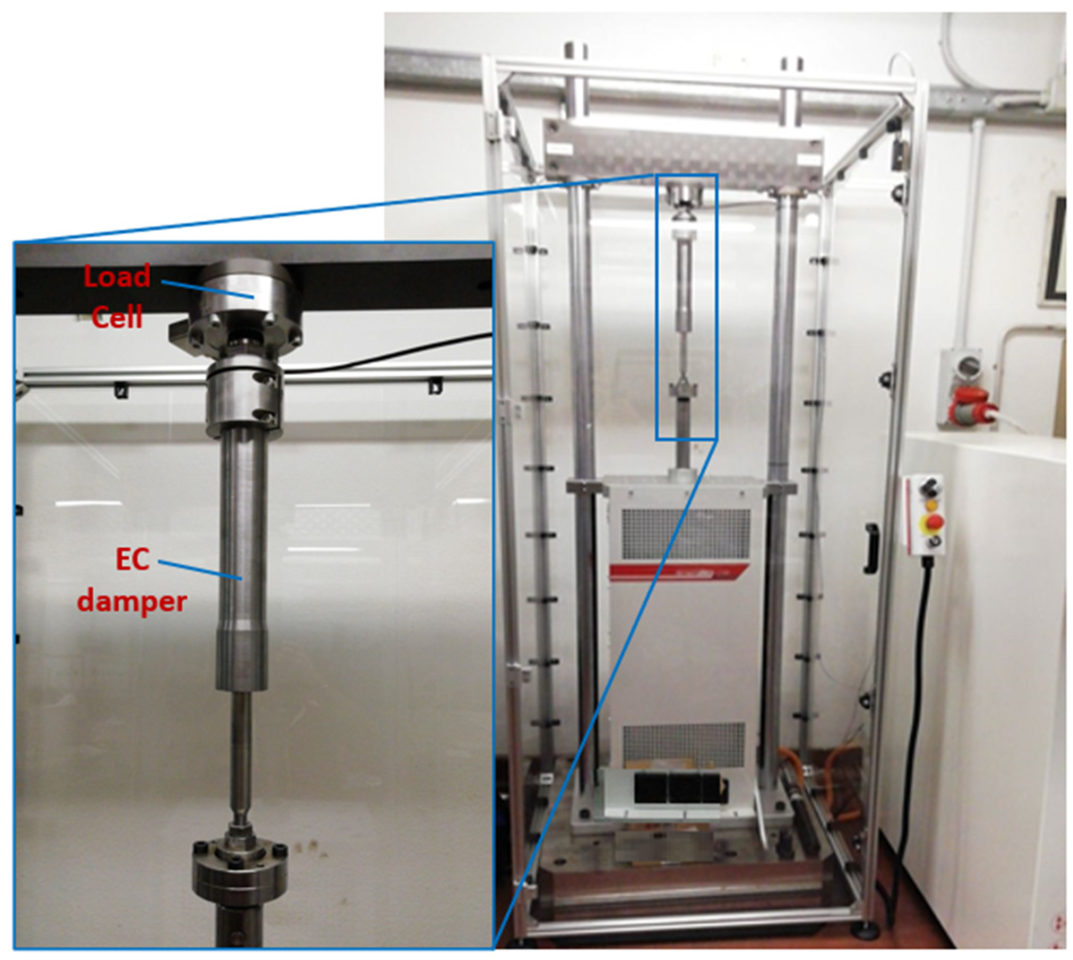
3. Experimental Validation of the EC Damper Model

We manufactured a prototype EC damper and carried out experiments on a test rig (Figure 5) to investigate its damping properties and to verify the accuracy of the FE model. Figure 5 shows the prototype EC damper mounted onto an ad hoc test rig designed and constructed by Step Lab Engineering S.r.l. (4 kN static and 14 kN dynamic forces, acceleration up to 35 g, stroke 210 mm and maximum speed of 4 m/s). Various sinusoidal and arbitrary displacement inputs of up to 100 Hz can be programmed.
The temperature of the external surface of the damper was measured using an infrared DT 8833 thermometer. The instrument has an optical resolution of 13:1 and basic accuracy of ±1.5% over the −50 to 800 °C range. The temperature of the surface was measured on the EC damper surface at the mid-stroke.

4. EC Damper Simulation and Experimental Results

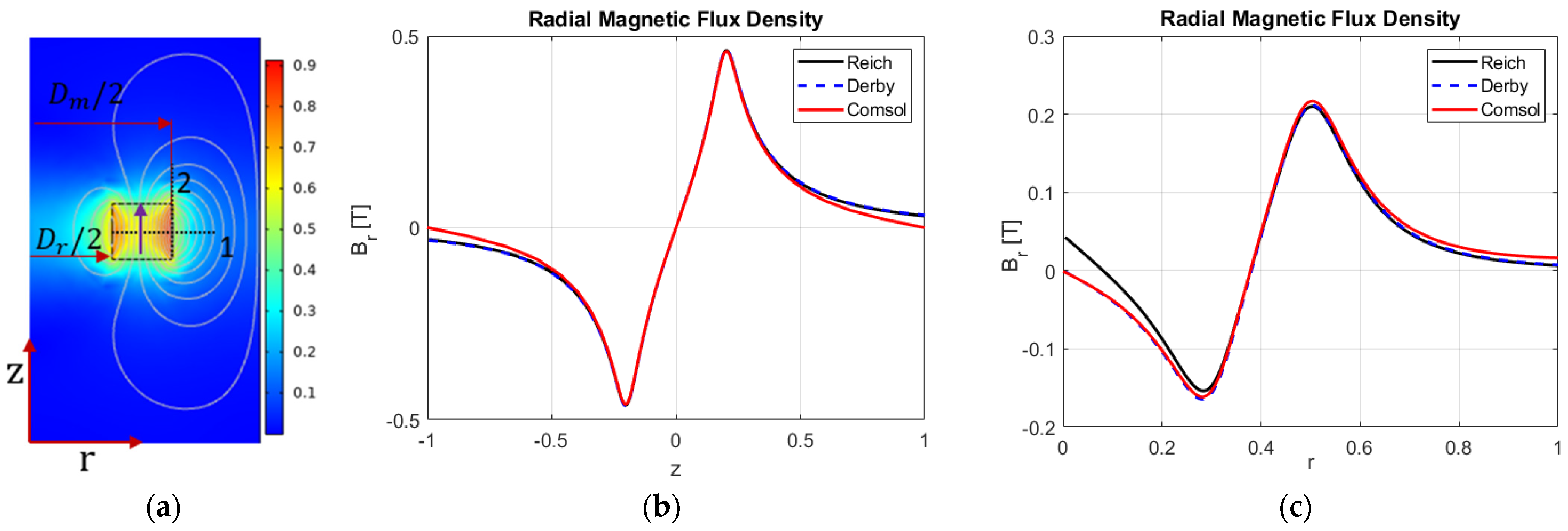
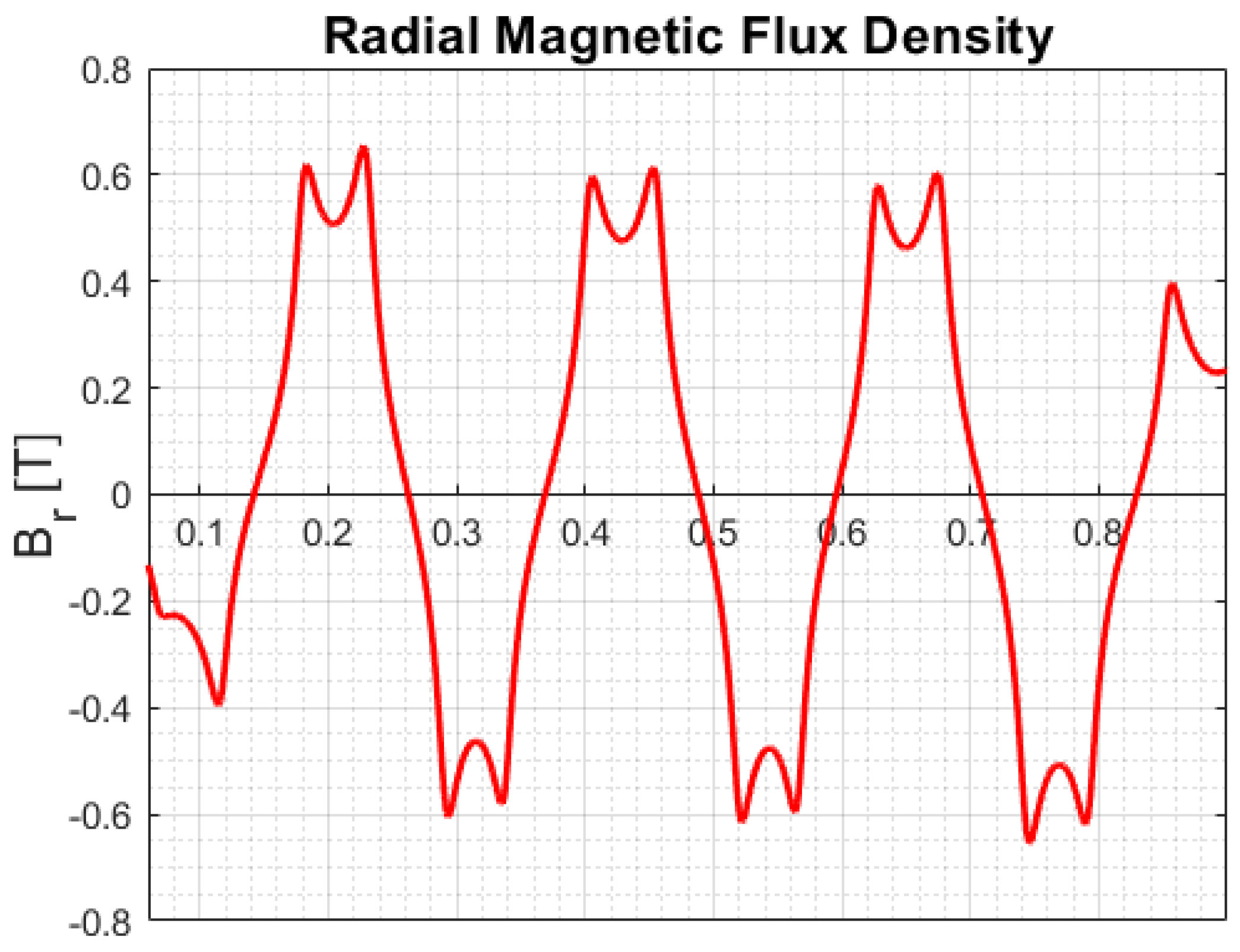
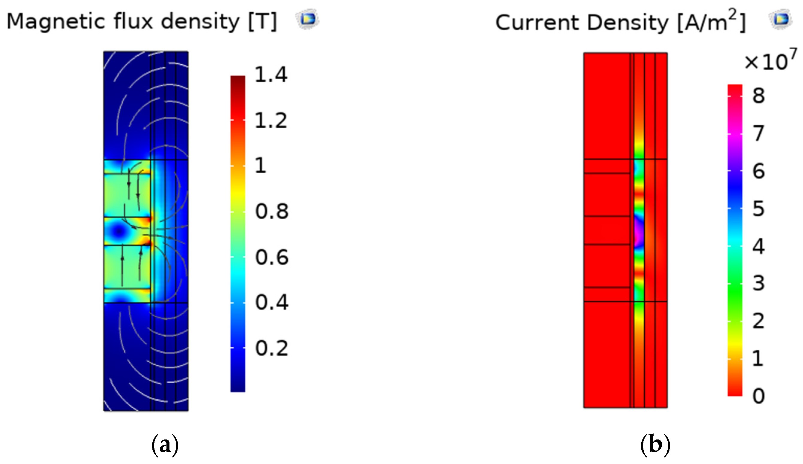
4.1. The Magnetic Field

Figure 6a shows the magnetic field around an axially magnetized PM (solid arrow). Directions 1 and 2 in the figure were selected to make FE comparisons against the literature [16,17], with reference to the results pertaining to the radial magnetic flux density. The results shown in Figure 6b,c demonstrate a close matching between FE and the analytical models in the literature.
As further proof of the model results, an effort was made to reproduce Figure 6 in reference [46] using FEM. The results, expressed in terms of the radial magnetic flux density along the conductor length at the mid-distance of the air gap, including IP effects, are shown in Figure 7 and are in good qualitative and quantitative agreement. Thus, our model can be considered for actual design purposes.
Figure 8 shows the magnetic field and the surface current density across a single module of the real EC damper. It should be noted that a real EC damper can be composed of several additional modules, depending on the desired damping force, without any significant changes in the designed module. The streamlines in Figure 8a indicate the direction of the field, while the current density in Figure 8b is generated over the conductor tube surface at 15 Hz.
Figure 8a also demonstrates that the IPs are prone to saturation, as the magnetic flux density across them is high. Therefore, the IP height, as well as the material, should be chosen so that magnetic choking is avoided.
Figure 9a compares the initial magnetization curves of the two candidate materials for the IP, i.e., Vacoflux (Fe − Co) alloy and Armco (99.85 wt.% Fe) pure iron. The saturation of the former was just above 2.3 T at room temperature, while the latter was 100% ferritic, with a saturation of 1.8 T.
In general, the cobalt content of Fe-Co alloys ranges from 15 to 50 wt.% and has a large Curie temperature and saturation magnetic flux density (up to 2.4 T at room temperature [22,47,48]). These unique properties are relevant for high temperature applications. The magnetic flux saturation may be increased by increasing the Co content (up to 40–45%) and the milling time [48]. Pure iron has good ferromagnetic properties and relatively poor electrical resistivity. It also demonstrates relatively low structural strength and hardness for external loads. Moreover, it is a cost-effective solution for IPs, whenever a high magnetic output is required.
Figure 9b shows the normalized damping coefficient C * as a function of the IP height-to-pole pitch ratio   ζ = τ i / τ p . The pole pitch height was kept constant, while the magnet and IP heights were varied. It should be noted that the magnetic saturation of the pole piece materials in the EC damper application determines their size and, thus, the specific magnetic output of the piston. Small values of ζ for the two investigated soft materials resulted in a somewhat large damping coefficient which, in turn, determined a greater saturation. The obtained damping performances appeared to be in favor of the Vacoflux alloy, although its market price currently hinders its widespread use in this field.
A different perspective view of Figure 9b is given in Figure 9c. The horizontal solid line arrows indicate the PM magnetization direction, while the oblique dotted line arrows indicate IPs. The smaller the height of the IPs is, the larger the magnitude of the radial flux density on the conductor surface and, according to Equation (4), the larger the damping force.
Electrically conductive materials dissipate electrical energy into heat. Previous findings indicate that a larger conductor thickness results in an increased damping coefficient [1]. In the present case, the selection of a copper conductor pipe has maximized the damping performance, but at the expense of a larger weight of the device than one in aluminum. Further efforts are required to minimize the conductor weight, while maximizing its damping performance. Figure 10a shows the computed damping coefficient obtained when varying the thickness of the conductor in a normalized manner, i.e., with respect to a baseline maximum thickness. The thickness ratio in Figure 10a is equal to 1 when the thickness coincides with the baseline thickness. Unlike previous research findings, a 30% decrease in the initial thickness (thickness ratio = 0.7) leads to an increase in damping and a corresponding decrease in the weight of the device. At the same time, the back iron thickness increases when the outer diameter of the conductor decreases (Dco, in Figure 1), and the magnetic field becomes more concentrated over the conductor. A further decrease in thickness (lower ratios than 0.7) results in even lower damping coefficients. The above results, which are based on a back iron congregation effect, agree well with those of reference [5].

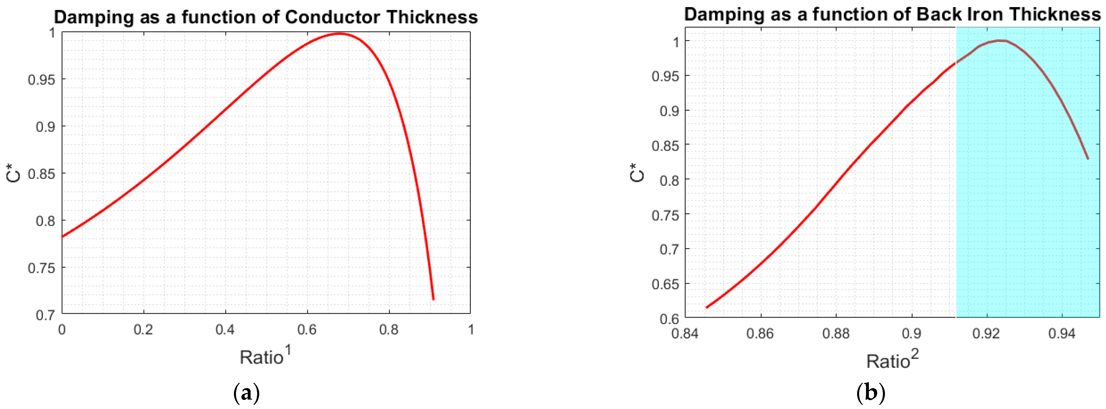
4.2. The Effect of Back Iron

The back iron and steel pipe in the EC damper, apart from serving as structural material, must close the magnetic circuit by eventually concentrating the magnetic field over the conductor. Iron losses originate in the iron, due to hysteresis, because of the alternating magnetic field. The relatively low thermal conductivities of iron and steel prevent the heat from being efficiently dissipated from the damper surfaces. This suggests the need for a systematic study on the effect of back iron on the damping coefficient. The ratio of the internal diameter (Dco) to the external diameter (Do) of the outer pipes (Figure 1) can be considered to be a design parameter that is worth optimizing. Assuming Do and the air gap ((Dci − Dm)/2) as constants, Dco and Dm were varied systematically, using the initial magnetization curve of the pure iron for both tube materials (assuming a single tube), as shown in Figure 10b. Although the achievable damping can reach its maximum value over the colored area, structural failure and material saturation are also likely to occur. Furthermore, back iron saturation is also observed in the same region after the peak is reached, where the magnetic flux lines pass through the ferromagnetic tubes and are lost in the space. Once the Dm had been fixed, a further increase in back iron pipe thickness did not generate any further damping, but just a weight increase of the device. However, the magnetic properties can rapidly deteriorate for higher temperatures and increased aging. Although the latter can occur in high-C structural steels (the external steel tube), aging deterioration may require several years before any remarkable changes take place.

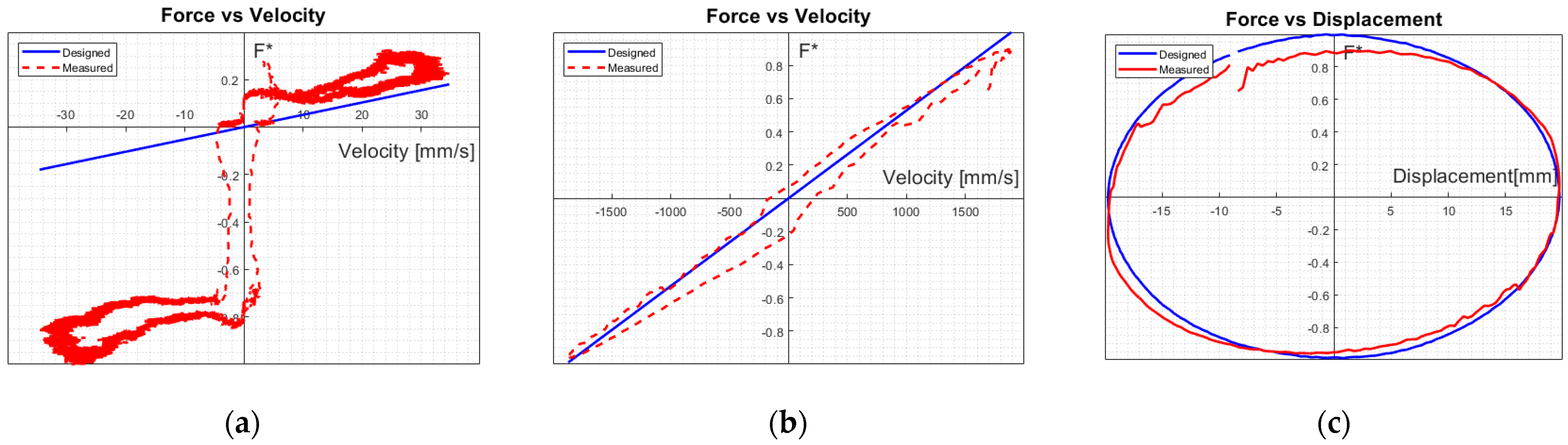
4.3. Performance of the EC Damper and Experimental Verification

The above systematic analysis, which was performed over the most relevant EC damper parameters, allowed us to define the most critical design factors. The optimization of such parameters permitted us to construct an EC damper prototype with the Quad geometrical constraints. The relative model was set up to help optimize its damping force. It was first experimentally calibrated and then verified against laboratory test rig data. The data consisted of force, displacement, velocity, acceleration and friction force recordings. The used test rig is shown in Figure 5. Figure 11a compares the force vs. velocity characteristics at 0.1 Hz. An assessment of very low frequency regimes, for example at 0.1 Hz, allowed us to detect any incipient dry sliding friction. The latter is in fact the main reason for any deviation between the simulated and measured characteristics. The friction force under tension loading was different from that under compression loading. The friction force can be further decreased by improving the shape and size tolerances during manufacturing. The curves are parallel to each other, except for the deviation at the origin of Figure 11a, and therefore share the same slope ( C * ).
On the other hand, the friction effect is difficult to perceive at higher frequencies, as can be noted in Figure 11b,c. The above comparisons reveal an excellent phenomenological agreement between the simulated and experimental characteristics for various working frequencies of practical interest, despite the friction effects.

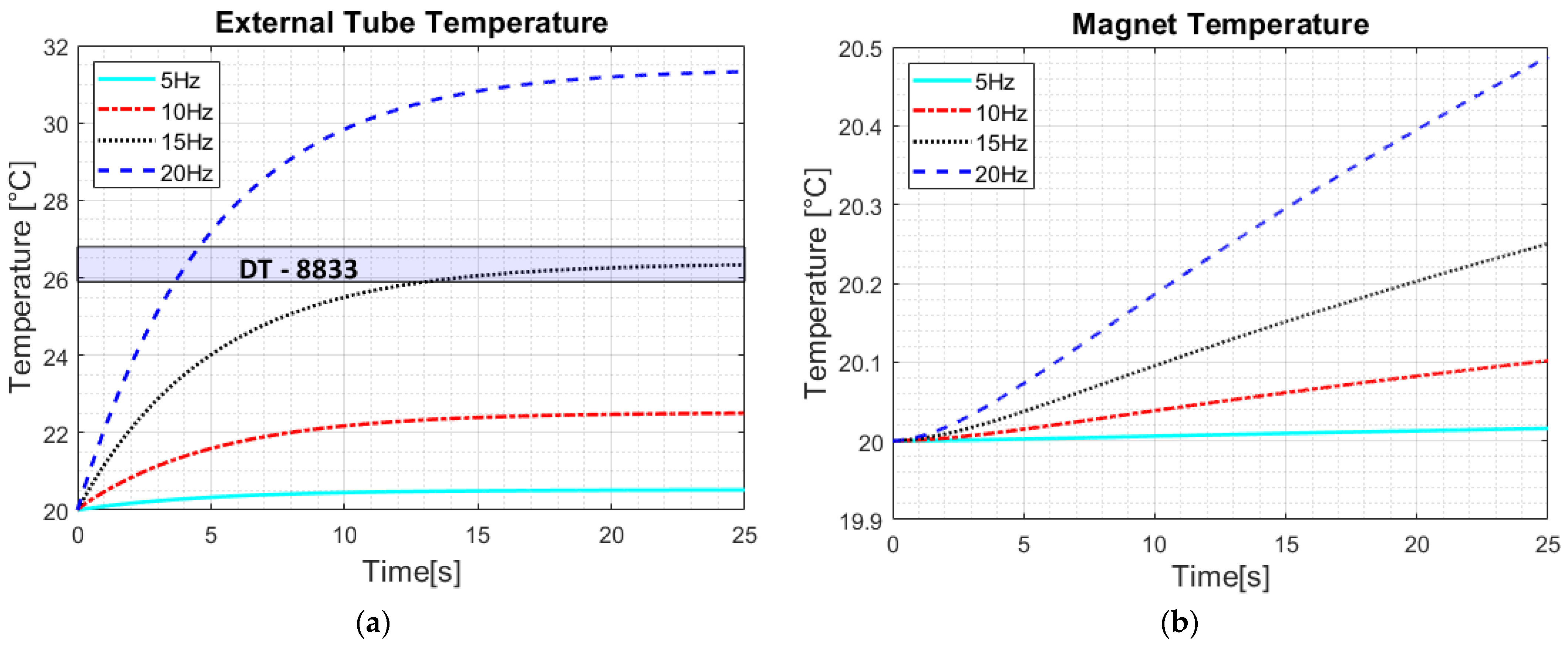
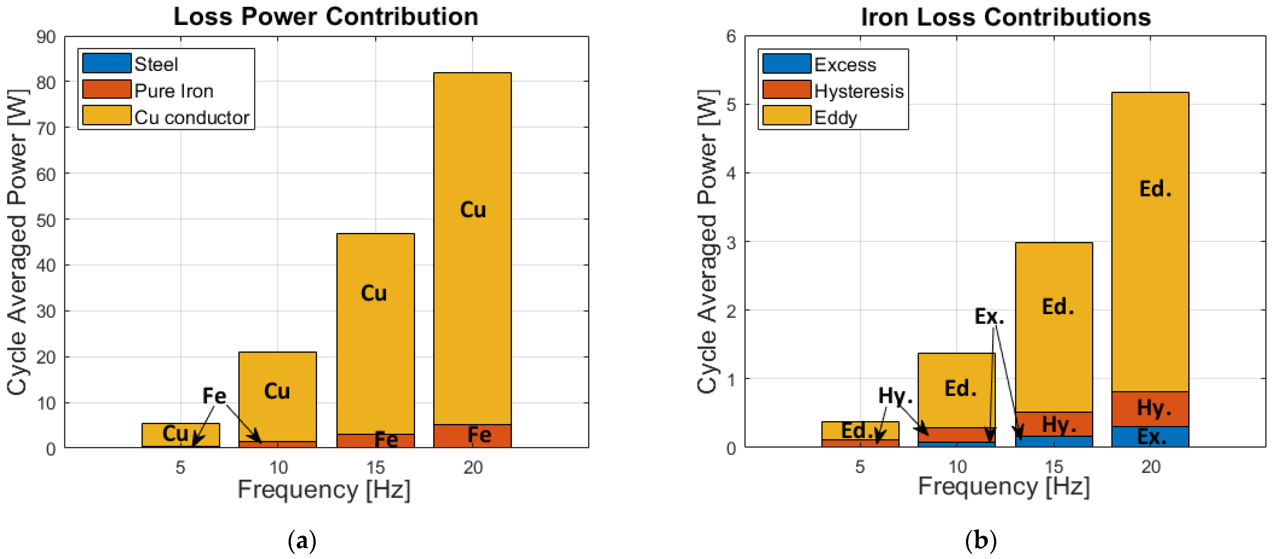
4.4. Thermal Characteristics

Figure 12a depicts the computed time-averaged spatial distribution of the volumetric electromagnetic losses per cycle at 15 Hz in the system. The losses include the resistive and hysteresis ones and are passed on to the thermal model via the input source term. The electromagnetic losses are more pronounced across the conductor pipe, as expected. Figure 12b shows the predicted temperature field for 15 Hz cycling after 26 s. Although a temperature peak was found in all the stator tubes, its low value suggests satisfactory design cooling conditions. Laboratory tests confirmed this value and the attainment of a steady-state condition. Figure 12 also shows the division of the stator pipes into three equal regions to measure the relative average temperatures. The region of major interest is the central one, as the maximum peak was designed to be located at the mid-stroke position.
Figure 13a shows the surface average temperature increase in the central portion of the tube for different frequencies. As can be observed, the temperature reaches a steady state, and the time necessary to reach a steady state increases with the frequency. The simulation was verified through laboratory measurements, using a DT 8833 thermometer after 30 s of excitation on the test rig, to attain a steady state at the mid-stroke position. The cross-hatched region in Figure 13a indicates the maximum and minimum experimental temperature ranges. In general, the damping force increases as the excitation frequency increases. Thus, the temperature also increases, due to the high level of heat dissipation. Figure 13b shows the average temperature increase in the PMs. The increase in the temperature rate is smaller than the sources indicated in Figure 13a. Its value is very low for the analyzed frequency ranges.
It is worth noting that the coupling between the magnetic and the thermal field is an important requirement for a safe design of any EC damper. This is true even when a weak coupling, such as the one considered in this study, is established. It should be recalled that the PM is a key component of an EC damper, and its individual performance has a direct impact on the overall performances of the EC damper. The performance of our PM dramatically decays for operating temperatures above 80 °C, as indicated in the supplier’s data sheet. Thus, the relatively low temperature values shown in Figure 12 and Figure 13 should be considered to be a final verification of a successful design stage, which means that all the important design factors considered in the analysis, such as the part geometry, material selection and device configuration are sound under the investigated operating condition, and that the PMs operate optimally. However, if a higher operating frequency range is necessary, the temperature field inside the EC damper can be expected to be more severe, and a new design strategy should therefore be analyzed to ensure that the inner temperatures are well below the PM degradation temperature. Thus, the thermal field cannot be excluded or separated from the magnetic field in a design analysis. Its inclusion in the design stage is the necessary price to pay to be able to assess that any change in geometry, material selection and/or operation conditions does not compromise the PM functions.
Figure 14a quantifies the role of the materials, in terms of the contribution of the losses calculated using Bertotti et al.’s power loss separation method. The losses are cycle-averaged for different frequencies. The losses in the steel tube appear to be negligible. As expected, the most crucial material in the EC damper is its conductor, and its contribution to the loss in energy is around 94% for all the studied frequency ranges. Figure 14b shows the different contributions of the losses in the soft materials of the EC damper stator. The hysteresis and excess losses are very small for low frequencies, as expected, but their contribution begins to increase as the frequency of the oscillations increases.

5. Discussion

A unique feature that is highlighted in this work is the use of back iron as an optimal design strategy to enhance the damping performances of an EC damper. The influence of back iron has not been studied before and has only been mentioned as an effective design factor that needed to be optimized [5] as it contributes to increasing the damping force. To better quantify the contribution of back iron in damping performances, we have taken into account the hysteresis effects in more detail. The hysteresis loop was introduced into the magnetic field model to more accurately account for the magnetic response and its thermal contribution, in terms of electromagnetic losses. The introduction of back iron in fact increased the normalized damping force per unit length (or volume), which is denoted as the damping force density, while it decreased the overall system mass. To point out the advantage of the back iron factor, we compared our design strategy (Figure 15) with that presented in ref. [1]. We then ad-hoc developed another finite element electromagnetic (Comsol) model, based on the data given in the previously mentioned reference, using original measured force-displacement results as input. However, these experimental results did not consider the influence of back iron. Hence, by comparing both model predictions, with and without back iron, we found that the performance of the EC damper improved as the thickness of the conductor decreased when back iron was introduced into the design strategy. Moreover, the undesired skin effect phenomenon was naturally avoided within the typical frequency range of automotive suspensions. The blue solid line in Figure 15 shows the damping force computed from the original parameters listed in Table 1, whereas the damper response at 45 Hz is shown in Figure 9a in the reference [1]. The profiles indicated in Figure 15 with blue stars, green triangles and black dashed lines describe the computed damping force attained for a variable thickness (i.e., tc = 1.5, 3 and 0.5 mm) in the case of a conductor made of pure aluminum. The results clearly highlight that a 1.5 mm thickness is optimal for the current design. A further increase or decrease in thickness would lower the damping force. Upon replacing the material conductor, i.e., using Al (37 MS/m) instead of Cu (58 MS/m), the damping force increases from 39.5 to 83.9 N for 45 Hz of excitation. Thus, the use of both a Cu conductor and back iron in an EC damper exerts more than a 3-fold increase in the damping force. Moreover, since the mass of the stator tube depends on its length, the above 3-fold improvement factor would also have a 38.2% reduction impact on the overall mass per unit length of the EC damper whenever a 1.5 mm thick tube assembly, made of Cu and back iron, is designed.
Another significant complexity of the EC damper model pertains to the CFD model used to account for the gas-flow interaction within the air gap. As the air gap is very narrow, the viscosity of the gas may be sufficient to increase the temperature of the magnets, therefore deteriorating their performance. Owing to the lack of precise experimental data, the choice of performing a full CFD analysis made it possible to overcome the stringent requirement of entering specific (unknown) input data related to the gas-flow conditions at the internal walls. In this case, it was only possible to perform the experimental validation by measuring the only accessible quantity, i.e., the average temperature over the outer surface of the steel tube. As this analysis just revealed an outer steady state wall temperature of 32 °C at 20 Hz, it can be concluded that a full CFD analysis is not essential for the present design, under the assumed operating conditions, and that the overall simulation time may be reduced to a great extent using appropriate empirical convective heat transfer correlations.
The developed EC damper model pertains to a smaller region than the actual one. This choice imposes the specification of periodic boundary conditions. In the present analysis, the periodic boundary condition is justifiable for the simulation of the magnetic field for the calculation of, for example, the damping force. However, periodic boundary conditions are not sufficiently reliable to fully account for the thermal phenomena as the air entrapped inside the gap may redistribute the developed heat. In our design, a constant temperature boundary condition was chosen at the two ends of the stator to mimic a long stator tube. The outer surface temperature was measured at the mid-stroke zone. Thus, if the two end-temperature walls were uncertain, then the attained simulation results should not be affected to any great extent. Furthermore, the assumed constant thermal material parameters have proved to be adequate, as the maximum predicted, and actual temperature did not exceed the values in the considered frequency range to a great extent.
This study has also highlighted important technological aspects regarding the optimal application of an EC damper in terrestrial vehicles. Even though the initial geometrical and mechanical constraints of the EC damper prototype were inspired by a simple and more economical McPherson strut, the present design shows that its application is more appropriate for a double wishbone type suspension, as the side force is somewhat detrimental for this device. Indeed, the only reason for selecting a McPherson type damper was related to the relatively easy and accessible instrumentation of QUAD for a quick and reliable setup of the developed EC damper design model.

6. Conclusions

A finite element-based methodology has been developed to optimally design the structure and the relative functions of an eddy current damper for automotive suspension, and an inherent systematic analysis has been conducted. First, the implementation of a hysteresis model with a Jiles-Atherton equation allowed an accurate prediction to be made of the magnetic field, and the relative iron losses were quantified for the first time using the loss separation model.
The magnetic model was successfully validated against model data taken from literature. A nonlinear magnetic electromagnetic analysis was then carried out, to assess the effectiveness of iron pole materials, by comparing the performance of two candidate materials. Next, the effects of thickness on the electromagnetic field across the conductor and back iron were optimized, in terms of both damping and mechanical resistance. A prototype was built, and the finite element model was validated against laboratory tests that measured the damping force for various operational frequencies. Finally, a coupled CFD-thermal model was set up to assess the heating effect on the permanent magnets at the same frequencies, and the accuracy of the loss separation model in the back iron was assessed against the mechanical vibration loss model. The overall thermal field has been verified by means of experimental tests. The proposed design has demonstrated the significant improvement (3-fold), in terms of damping force, and a decrease in the stator tube mass, by more than 38%, when back iron was used.
The EC damper technology is more beneficial when applied to double wishbone suspension than to the Mac-Pherson type, as the side forces in the former are considered to be negligible.
The developed methodology could also be applied for the design of linear motors and generators to increase their efficiency by decreasing any unwanted losses.

Author Contributions

Conceptualization, G.M.; methodology, G.M. and U.J.; software, U.J.; validation, G.M. and U.J.; formal analysis, G.M. and U.J.; investigation, G.M. and U.J.; resources, G.M.; data curation, U.J.; writing—original draft preparation, G.M. and U.J.; writing—review and editing, G.M. and U.J.; visualization, U.J.; supervision, G.M.; project administration, G.M.; funding acquisition, G.M. All authors have read and agreed to the published version of the manuscript.

Funding

This research received no external funding.

Institutional Review Board Statement

Not applicable.

Informed Consent Statement

Not applicable.

Acknowledgments

The authors would like to acknowledge the sincere efforts and valuable time given by their respected colleagues Frediano De Marco and Renato Pero. Their invaluable advice has helped to complete this article.

Conflicts of Interest

The authors declare no conflict of interest.

References

  1. Ebrahimi, B.; Khamesee, M.B.; Golnaraghi, F. Eddy current damper feasibility in automobile suspension: Modeling, simulation and testing. Smart Mater. Struct. 2008, 18, 015017. [Google Scholar] [CrossRef]
  2. Ebrahimi, B.; Khamesee, M.B.; Golnaraghi, F. A novel eddy current damper: Theory and experiment. J. Phys. D Appl. Phys. 2009, 42, 075001. [Google Scholar] [CrossRef]
  3. Abdo, T.M.; Huzayyin, A.A.; Abdallah, A.A.; Adly, A.A. Characteristics and Analysis of an Eddy Current Shock Absorber Damper Using Finite Element Analysis. Actuators 2019, 8, 77. [Google Scholar] [CrossRef] [Green Version]
  4. Maddah, A.A.; Hojjat, Y.; Karafi, M.R.; Ashory, M.R. Reduction of magneto rheological dampers stiffness by incorporating of an eddy current damper. J. Sound Vib. 2017, 396, 51–68. [Google Scholar] [CrossRef]
  5. Pu, H.; Li, J.; Wang, M.; Huang, Y.; Zhao, J.; Yuan, S.; Peng, Y.; Xie, S.; Luo, J.; Sun, Y. Optimum design of an eddy current damper considering the magnetic congregation effect. J. Phys. D Appl. Phys. 2019, 53, 115002. [Google Scholar] [CrossRef]
  6. Zhang, H.; Chen, Z.; Hua, X.; Huang, Z.; Niu, H. Design and dynamic characterization of a large-scale eddy current damper with enhanced performance for vibration control. Mech. Syst. Signal Process. 2020, 145, 106879. [Google Scholar] [CrossRef]
  7. Firoozy, P.; Friswell, M.I.; Gao, Q. Using time delay in the nonlinear oscillations of magnetic levitation for simultaneous energy harvesting and vibration suppression. Int. J. Mech. Sci. 2019, 163, 105098. [Google Scholar] [CrossRef]
  8. Kamaruzaman, N.A.; Robertson, W.S.; Ghayesh, M.H.; Cazzolato, B.S.; Zander, A.C. Six degree of freedom quasi-zero stiffness magnetic spring with active control: Theoretical analysis of passive versus active stability for vibration isolation. J. Sound Vib. 2021, 502, 116086. [Google Scholar] [CrossRef]
  9. Gulec, M.; Aydin, M.; Nerg, J.; Lindh, P.; Pyrhonen, J.J. Magneto-Thermal Analysis of an Axial-Flux Permanent-Magnet-Assisted Eddy-Current Brake at High-Temperature Working Conditions. IEEE Trans. Ind. Electron. 2020, 68, 5112–5121. [Google Scholar] [CrossRef]
  10. Zhao, X.; Zhang, Y.; Ye, L. Braking Torque Analysis and Control Method of a New Motor with Eddy-Current Braking and Heating System for Electric Vehicle. Int. J. Automot. Technol. 2021, 22, 1159–1168. [Google Scholar] [CrossRef]
  11. Diez-Jimenez, E.; Cordero, C.A.; Alcover-Sánchez, R.; Corral-Abad, E. Modelling and Test of an Integrated Magnetic Spring-Eddy Current Damper for Space Applications. Actuators 2021, 10, 8. [Google Scholar] [CrossRef]
  12. Ao, W.K.; Reynolds, P. Analytical and experimental study of eddy current damper for vibration suppression in a footbridge structure. In Dynamics of Civil Structures; Springer: Cham, Switzerland, 2017; Volume 2, pp. 131–138. [Google Scholar]
  13. Irazu, L.; Elejabarrieta, M.J. Analysis and numerical modelling of eddy current damper for vibration problems. J. Sound Vib. 2018, 426, 75–89. [Google Scholar] [CrossRef]
  14. Gysen, B.L.; van der Sande, T.P.; Paulides, J.J.; Lomonova, E.A. Efficiency of a regenerative direct-drive electromagnetic active suspension. IEEE Trans. Veh. Technol. 2011, 60, 1384–1393. [Google Scholar] [CrossRef] [Green Version]
  15. Callaghan, E.E.; Maslen, S.H. The Magnetic Field of a Finite Solenoid; National Aeronautics and Space Administration: Washington, DC, USA, 1960.
  16. Derby, N.; Olbert, S. Cylindrical magnets and ideal solenoids. Am. J. Phys. 2010, 78, 229–235. [Google Scholar] [CrossRef] [Green Version]
  17. Reich, F.A.; Stahn, O.; Müller, W.H. The magnetic field of a permanent hollow cylindrical magnet. Contin. Mech. Thermodyn. 2015, 28, 1435–1444. [Google Scholar] [CrossRef]
  18. MacLatchy, C.S.; Backman, P.; Bogan, L. A quantitative magnetic braking experiment. Am. J. Phys. 1993, 61, 1096–1101. [Google Scholar] [CrossRef]
  19. Bae, J.-S.; Hwang, J.-H.; Park, J.-S.; Kwag, D.-G. Modeling and experiments on eddy current damping caused by a permanent magnet in a conductive tube. J. Mech. Sci. Technol. 2009, 23, 3024–3035. [Google Scholar] [CrossRef]
  20. Friedrich, L.A.J.; Paulides, J.J.H.; Lomonova, E.A. Modeling and Optimization of a Tubular Generator for Vibration Energy Harvesting Application. IEEE Trans. Magn. 2017, 53, 1–4. [Google Scholar] [CrossRef]
  21. O’handley, R.C. Modern Magnetic Materials: Principles and Applications; Wiley: New York, NY, USA, 2000. [Google Scholar]
  22. Shokrollahi, H. The magnetic and structural properties of the most important alloys of iron produced by mechanical alloying. Mater. Des. 2009, 30, 3374–3387. [Google Scholar] [CrossRef]
  23. Du, S.W.; Ramanujan, R.V. Mechanical alloying of Fe–Ni based nanostructured magnetic materials. J. Magn. Magn. Mater. 2005, 292, 286–298. [Google Scholar] [CrossRef]
  24. Naumoski, H.; Maucher, A.; Herr, U. Investigation of the influence of global stresses and strains on the magnetic properties of electrical steels with varying alloying content and grain size. In Proceedings of the 2015 5th International Electric Drives Production Conference (EDPC), Nuremberg, Germany, 15–16 September 2015; pp. 1–8. [Google Scholar]
  25. Bertotti, G.; Fiorillo, F.; Soardo, G.P. The prediction of power losses in soft magnetic materials. J. Phys. Colloq. 1988, 49, C8-1915. [Google Scholar] [CrossRef]
  26. Zhu, Z.Q.; Xue, S.; Chu, W.; Feng, J.; Guo, S.; Chen, Z.; Peng, J. Evaluation of iron loss models in electrical machines. IEEE Trans. Ind. Appl. 2018, 55, 1461–1472. [Google Scholar] [CrossRef]
  27. Boglietti, A.; Cavagnino, A.; Lazzari, M.; Pastorelli, M. Predicting iron losses in soft magnetic materials with arbitrary voltage supply: An engineering approach. IEEE Trans. Magn. 2003, 39, 981–989. [Google Scholar] [CrossRef]
  28. Kowal, D.; Sergeant, P.; Dupre, L.; Vandenbossche, L. Comparison of Iron Loss Models for Electrical Machines with Different Frequency Domain and Time Domain Methods for Excess Loss Prediction. IEEE Trans. Magn. 2014, 51, 1–10. [Google Scholar] [CrossRef]
  29. Bottauscio, O.; Canova, A.; Chiampi, M.; Repetto, M. Iron losses in electrical machines: Influence of different material models. IEEE Trans. Magn. 2002, 38, 805–808. [Google Scholar] [CrossRef]
  30. Jiles, D.C.; Atherton, D.L. Theory of ferromagnetic hysteresis. J. Appl. Phys. 1984, 55, 2115–2120. [Google Scholar] [CrossRef]
  31. Leite, J.V.; Benabou, A.; Sadowski, N. Accurate minor loops calculation with a modified Jiles-Atherton hysteresis model. COMPEL-Int. J. Comput. Math. Electr. Electron. Eng. 2009, 28, 741–749. [Google Scholar] [CrossRef] [Green Version]
  32. Szewczyk, R. Computational problems connected with Jiles-Atherton model of magnetic hysteresis. In Recent Advances in Automation, Robotics and Measuring Techniques; Springer: Cham, Switzerland, 2014; pp. 275–283. [Google Scholar]
  33. Podbereznaya, I.B.; Medvedev, V.V.; Pavlenko, A.V.; Bol’shenko, I.A. Selection of optimal parameters for the Jiles–Atherton magnetic hysteresis model. Russ. Electr. Eng. 2019, 90, 80–85. [Google Scholar] [CrossRef]
  34. Sedira, D.; Gabi, Y.; Kedous-Lebouc, A.; Jacob, K.; Wolter, B.; Strass, B. ABC method for hysteresis model parameters identification. J. Magn. Magn. Mater. 2020, 505, 166724. [Google Scholar] [CrossRef]
  35. Zou, M. Parameter estimation of extended Jiles–Atherton hysteresis model based on ISFLA. IET Electr. Power Appl. 2019, 14, 212–219. [Google Scholar] [CrossRef]
  36. Hergli, K.; Marouani, H.; Zidi, M. Numerical determination of Jiles-Atherton hysteresis parameters: Magnetic behavior under mechanical deformation. Phys. B Condens. Matter 2018, 549, 74–81. [Google Scholar] [CrossRef]
  37. Szewczyk, R.; Salach, J.; Bienkowski, A.; Frydrych, P.; Kolano-Burian, A. Application of Extended Jiles–Atherton Model for Modeling the Magnetic Characteristics of Fe41.5Co41.5Nb3Cu1B13 Alloy in As-Quenched and Nanocrystalline State. IEEE Trans. Magn. 2012, 48, 1389–1392. [Google Scholar] [CrossRef]
  38. Hussain, S.; Benabou, A.; Clenet, S.; Lowther, D.A. Temperature Dependence in the Jiles–Atherton Model for Non-Oriented Electrical Steels: An Engineering Approach. IEEE Trans. Magn. 2018, 54, 1–5. [Google Scholar] [CrossRef]
  39. Belgasmi, I.; Hamimid, M. Accurate Hysteresis Loops Calculation Under the Frequency Effect Using the Inverse Jiles-Atherton Model. Adv. Electromagn. 2020, 9, 93–98. [Google Scholar] [CrossRef]
  40. Reimpell, J.; Stoll, H.; Betzler, J. The Automotive Chassis: Engineering Principles; Elsevier Butterworth-Heinemann: Oxford, UK, 2001. [Google Scholar]
  41. Jiles, D.C.; Thoelke, J.B.; Devine, M.K. Numerical determination of hysteresis parameters for the modeling of magnetic properties using the theory of ferromagnetic hysteresis. IEEE Trans. Magn. 1992, 28, 27–35. [Google Scholar] [CrossRef]
  42. Sablik, M.J.; Kwun, H.; Burkhardt, G.L.; Jiles, D.C. Model for the effect of tensile and compressive stress on ferromagnetic hysteresis. J. Appl. Phys. 1987, 61, 3799–3801. [Google Scholar] [CrossRef]
  43. Bergman, T.L.; Lavine, A.S.; Incropera, F.P.; DeWitt, D.P. Fundamentals of Heat and Mass Transfer, 7th ed.; John Wiley & Sons: Hoboken, NJ, USA, 2011. [Google Scholar]
  44. Available online: https://www.comsol.com/model/download/735431/models.acdc.vector_hysteresis_modeling.pdf (accessed on 1 November 2021).
  45. Ebrahimi, B.; Khamesee, M.B.; Golnaraghi, F. Permanent magnet configuration in design of an eddy current damper. Microsyst. Technol. 2010, 16, 19. [Google Scholar] [CrossRef]
  46. Gieras, J.F.; Piech, Z.J.; Tomczuk, B. Linear Synchronous Motors: Transportation and Automation Systems, 2nd ed.; CRC Press: Boca Raton, FL, USA, 2012. [Google Scholar]
  47. Bas, J.A.; Calero, J.A.; Dougan, M.J. Sintered soft magnetic materials. Properties and applications. J. Magn. Magn. Mater. 2003, 254, 391–398. [Google Scholar] [CrossRef]
  48. Chermahini, M.D.; Zandrahimi, M.; Shokrollahi, H.; Sharafi, S. The effect of milling time and composition on microstructural and magnetic properties of nanostructured Fe-Co alloys. J. Alloys Compd. 2009, 477, 45–50. [Google Scholar] [CrossRef]
Figure 1. Schematics of the EC damper (cross section view).
Energies 15 01147 g001
Figure 2. Hysteresis loops of the SAE 4340 steel and ARMCO pure iron. The inset shows a magnifcation of the loop at the origin.
Energies 15 01147 g002
Figure 3. Field (module) coupling and Multiphysics flow of the finite element EC damper model.
Energies 15 01147 g003
Figure 4. Mesh sensitivity to the normalized damping force vs. velocity of the piston; the number of elements is shown in the legend.
Energies 15 01147 g004
Figure 5. The Laboratory test rig used to experimentally validate the EC damper FE model prototype.
Energies 15 01147 g005
Figure 6. Validation of the EC damper model against literature models [16,17], in terms of the radial magnetic flux density: (a) axisymmetric magnetic flux distribution across the PM: the solid purple arrow indicates the magnetization direction; (b) along positive direction 1; (c) along positive direction 2 in the PM.
Energies 15 01147 g006
Figure 7. Reproduced predicted radial magnetic flux density profile along the conductor length at the midline of the air gap from ref. [46], used here for validation purpose.
Energies 15 01147 g007
Figure 8. The reference (see Figure 1 for reference) EC damper model computed (a) magnetic; (b) current density fields across it at 15 Hz.
Energies 15 01147 g008
Figure 9. The IP material and thickness effects on damping: (a) initial magnetization curves of the investigated soft magnetic materials; (b) the normalized damping coefficient of the two investigated materials vs. ζ-the IP height-to-pole pitch ratio; (c) radial magnetic flux density on the surface of the conductor along its length vs. ζ-the IP height-to-pole pitch ratio, with a pure iron magnetization curve.
Energies 15 01147 g009
Figure 10. Conductor and back iron thickness effects: (a) Normalized damping coefficient vs. normalized conductor thickness ( Ratio 1 ); (b) normalized damping coefficient vs. normalized back iron thickness ( Ratio 2 ). The colored region cannot be used due to structural constraints.
Energies 15 01147 g010
Figure 11. Characteristics of the (a) force–velocity at 0.1 Hz (b) force-velocity at 15 Hz; (c) force-displacement at 15 Hz: comparison between the measurements (laboratory test rig) and predictions (FE EC damper model).
Energies 15 01147 g011
Figure 12. (a) Cycle-averaged volumetric electromagnetic power losses and (b) the steady-state temperature field at 15 Hz.
Energies 15 01147 g012
Figure 13. Temperature history (a) over the external steel tube surface at the mid-stroke position; (b) across the PMs for various frequencies.
Energies 15 01147 g013
Figure 14. Contribution of the power losses for various frequencies in (a) the stator materials; (b) the soft magnetic materials of the stator.
Energies 15 01147 g014
Figure 15. Influence of the damping force on the EC damper from ref. [1] with the contribution of back iron.
Energies 15 01147 g015
Table 1. Main parts and parameters of the EC damper.
SymbolName
D r Rod diameter
D m Magnet outer diameter
D io Pure iron outer diameter
τ p Pole pitch
D ci Cu tube—inner diameter
D co Cu tube—outer diameter
D o Damper—outer diameter
τ i Iron pole height
Table 2. EC damper material properties.
MaterialElectrical Resistivity [Ωm] Thermal   Conductivity   [ W mK ] Heat   Capacity   [ J kgK ]
Cu–ETP tube1.67 × 10−8390385
ARMCO iron10.51 × 10−873.2450
SAE 4340 steel24.8 × 10−844.5475
Neodymium PM1.2 × 10−48.95502
Inconel 7181.25 × 10−611.4435
Table 3. Discretized geometry and corresponding number of assessed finite elements.
Number of Elements928112212351703364311,716
Energies 15 01147 i001 Energies 15 01147 i002 Energies 15 01147 i003 Energies 15 01147 i004 Energies 15 01147 i005 Energies 15 01147 i006
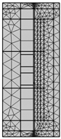
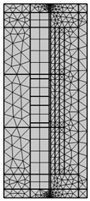
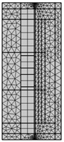
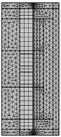
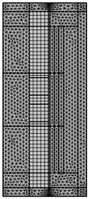
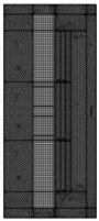
Publisher’s Note: MDPI stays neutral with regard to jurisdictional claims in published maps and institutional affiliations.

