Machine Learning to Rate and Predict the Efficiency of Waterflooding for Oil Production

Abstract

Waterflooding is a widely used secondary oil recovery technique. The oil and gas industry uses a complex reservoir numerical simulation and reservoir engineering analysis to forecast production curves from waterflooding projects. The application of such standard methods at the stage of assessing the potential of a huge number of projects could be computationally inefficient and requires a lot of effort. This paper demonstrates the applicability of machine learning to rate the outcome of waterflooding applied to an oil reservoir. We also explore the relationship of project evaluations by operators at the final stages with several performance metrics for forecasting. Real data about several thousand waterflooding projects in Texas are used in the current study. We compare the ML models rankings of the waterflooding efficiency and the expert rankings. Linear regression models along with neural networks and gradient boosting on decision threes are considered. We show that machine learning models allow reducing computational complexity and can be useful for rating the reservoirs, with respect to the effectiveness of waterflooding.

1. Introduction

Waterflooding is a very effective oil recovery improvement technique. This technique began at the beginning of the 20th century, but it is still popular—and widely used—in the vast majority of oil fields. Waterflooding is a secondary oil recovery technique in which water is injected into the reservoir formation to displace residual oil. The water from injection wells physically sweep the displaced oil to adjacent production wells. It allows improving the recovery of oil and maintaining reservoir pressure. The method increases oil recovery from 20% to 40% of the original oil in place on average [1]. However, many secondary waterflooding attempts have failed due to a paucity of data or inept assessment failed to disclose the true nature of the prospect [2]. The effect of waterflooding is critically affected by characteristics of the reservoir (geological structure, internal architecture, properties of reservoir rock and fluids) and the specifics of the oilfield development scheme. For successful investment it is necessary to assess the prospects of the project in advance and choose the most potentially successful ones.

The success and efficiency of waterflooding depends on many characteristics of both the reservoir and development parameters. It could strongly depend on the previous reservoir performance, lateral and vertical permeability, porosity distribution, residual oil, mobility ratio, well spacing, and other parameters. Nowadays, various methods are used in practice for oil recovery performance forecast. All commonly used methods can generally be divided into reservoir numerical simulations and reservoir engineering analyses [3,4].

To consider all of the effects of the physics process, a full-scale 3D reservoir numerical simulation could be used. This approach allows simulating the process as realistic as possible, solving differential equations numerically. However, in order to obtain accurate results, much effort is required to collect data to build and validate a sufficiently accurate reservoir model. For a large-scale or complex reservoir simulation model, a single forward simulation run can take from several hours to several days to complete [5]. To accelerate the simulation, recent studies have considered replacing the full-scale reservoir simulation model with a far more computationally efficient surrogate or proxy model, such as reduced order modeling (ROM) [6] or methods based on deep neural networks [7]. However, the development of such a model requires comprehensive geological modeling and fine tuning to obtain acceptable accuracy.

The reservoir engineering methods are used to speed up the simulation. One can use models based on the material balance equation for the entire reservoir or its hydrodynamically isolated parts [5,8]. Another example is the capacitance–resistance model (CRM) [9,10]. CRM model estimates interwell connectivity between each water injection well. These methods typically require production and injection history as well as bottomhole pressure. Fine-tuning made by a highly experienced specialist is usually necessary to obtain satisfactory results.

The application of such standard methods at the stage of assessing the potential of a project requires a lot of effort. There may be insufficient data in the early stages to apply complex physics-based models. In addition, the forecast of the production curves may be unnecessary. This is especially evident where, among hundreds of potential projects, the most promising ones should be selected. Often, all available information represents the averaged reservoirs characteristics. Such parameters refer to reservoir geometry, geology, transport, and fluid properties. Using these data, project effects need to be assessed as accurately as possible.

To select the most successful candidates, it is necessary to rank the potential IOR projects according to the efficiency metrics estimated with some models. These effect metrics are various. The most commonly used is secondary ultimate oil/primary ultimate oil [11]. Substitution Index (SI), expected ultimate recovery (EUR), and similar, are also mentioned in the literature [12,13,14]. The data-driven ML approach, having relatively rich historical training data, is suitable for estimating valuable performance metrics for waterflooding projects. One can build a model that takes a given set of parameters as input and predict various target values that can be useful in risk assessment analysis. (for example oil rate leap or years to extract 80% of secondary oil). Data-driven models are starting to be used for similar tasks. A number of studies confirmed the effectiveness of ML models in application to oil recovery factor estimation [14,15,16]. Several other studies have reported the successful application of ML models to estimate the effects of hydraulic fracturing [17,18,19,20]. Kornkosky et al. applied multivariate linear regression to estimate the waterflooding effect [11]. The authors demonstrated low accuracy of the linear model.

In this study, our goal was to relate several waterflooding project metrics to real operator effect evaluations made in the final stages of waterflooding projects; to show the flexibility and practical applicability of advanced machine learning techniques, to assess the potential of secondary oil recovery projects. We used an open database with 8600 IOR projects of Texas oilfields. In the Methodology Section 2, we describe in detail the dataset, its features, and available data. Next, we describe an approach to recover production curves from data to calculate additional effect metrics and analyze the operator’s evaluations. Finally, we describe the applied ML models and how we measured the accuracy. In the Results Section 3, we report on the restored production curve accuracy analysis, the comparison of the operator’s evaluations with curve shapes and the project’s effect metrics, and an evaluation of ML models. In the Section 4 and Section 5, we highlight the most interesting findings, discuss the pros and cons of a data-driven approach, limitations of the results, and state future research directions.

2. Materials and Methods

In this section, we describe the data and methods. The first subsection is devoted to the data we used to train the ML models to predict the waterflooding project effects. We briefly demonstrate the organization of tables and their relationships and what types of projects the database contains. We also illustrate the typical timeline of the project and what data are available at each stage. In the following subsection, we explain which effect metrics we chose to predict and how we investigated as to whether the operator’s effect evaluation was consistent with the chosen metrics. We also describe the method of restoring production curves from database parameters (it helped us analyze the nature of the operator’s evaluation and calculate several useful effect metrics to predict). In the last subsection, we discuss the process of filtering data to form a training sample and describe the applied ML models and tuning details. Finally, we explain how we measured the quality of the data-driven models: how we measured the accuracy of the models and the method to compare the model with the operator’s assessment of the project.

2.1. Dataset Description

In this study, we used data from the Texas Secondary & Enhanced Recovery Database (Bulletin 82) [11,21]. The database has records on more than 8600 improved oil recovery projects in Texas from 1950–1982. It includes more than 80 different types of data on each one. Not all items are complete for each project. The average missing value rate for one item is about 50%. However, there are items with even 90–100%. The data are organized into five separate files, with only the project number common to each file.

We considered projects related to waterflooding only. We also considered areas where only one project was made in order to exclude the influence of other projects on the effect.

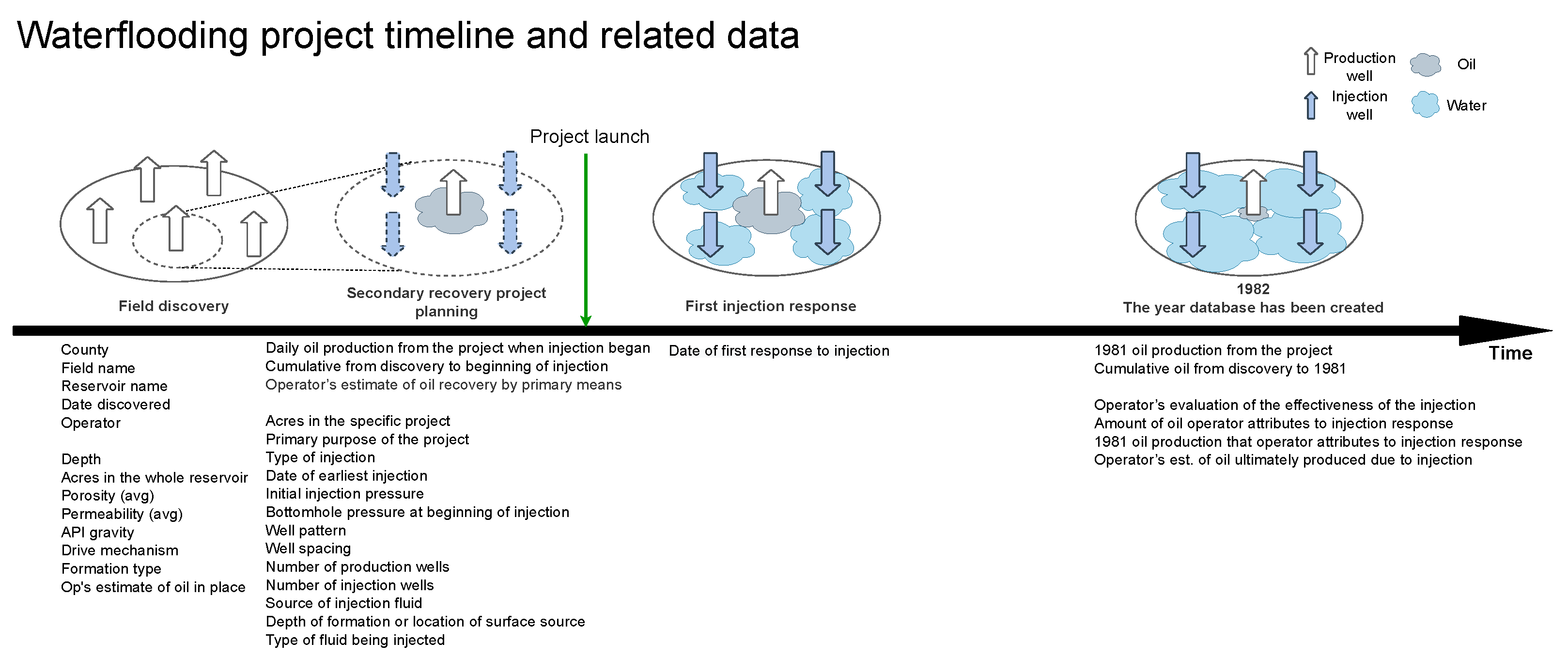
2.2. Waterflooding Project Timeline

Waterflooding projects were launched at various times and the last database update was in 1982. It is necessary to distinguish at what stages of the project certain data were available. We divided all parameters we used into two group: known before the project was launched and known during the project (mainly related to 1982). The first group contains parameters related to reservoir location, averaged parameters related to geometry, geology, transport properties, and fluid properties. It also contains several development parameters, which were known at the planning stage of the project. The second group contains parameters related to project performance. Figure 1 demonstrates the typical waterflooding project timeline data availability at every stage.

Parameters from the first group can be used as input parameters for the ML model to predict the effect of the project. We used parameters from the second group to calculate waterflooding effect metrics.

2.3. Waterflooding Effect Metrics

The main purpose of this study was to develop and evaluate the data-driven model to estimate the effects of waterflooding projects using parameters known before the project started. We can express the effect of the project in the form of some metric, i.e., as a numeric value. This metric should reflect the economic potential of the project and be useful in decision-making. This approach could help with selecting the most cost-effective among several potential projects.

The database we used contains an operator’s evaluation of the injection effectiveness. An assessment was made by an operator after a project started. The corresponding data field is categorical and could take one of the following values “NOT EFF”, “MODERATE”, and “VERY”. Although this metric reflects the project’s performance, the range of values is very narrow, which could make the decision-making process difficult. There is also no information about what the operator was guided by when making a decision and what characteristics were important. Therefore, we aimed to use several other numerical values as targets. Firstly, we wanted to demonstrate that, with a date-driven approach, it is possible to train a model for any metric, and secondly, in various economic situations, different characteristics could be important.

Using source data, we calculated and used as a target the following metric, which is quite natural and widely used for assessing the potential of secondary recovery projects [11]:

• Secondary ultimate oil/primary ultimate oil.

This metric represents the ratio of oil attributed to waterflooding to oil produced by depletion drive. This metric could be valuable for comparing the economic costs of the project with the potential profit.

The other two metrics are presented below:

• Oil rate leap.
• Years to extract 80% of oil attributed to secondary recovery.

The second one represents the largest increase in oil production. This effect metric can be useful in predicting when it is necessary to raise oil production rates as soon as possible. The third one reflects the duration of the project and can be valuable in long-term economic forecasts.

2.4. Oil Production Curves Estimation

With several parameters from the database, we tried to restore production curves using the decline curve analysis. To approximate primary production curves, we used the exponential rate–time relationship proposed by Arps et al [22]. Similarly, we used a simple parametric model, e.g., the diffusivity-filter, to approximate the secondary production curves [23,24,25].

2.4.1. Primary Oil Recovery Curve

For oil rate attributed to the depletion drive, we used a simple exponential relationship with a constant loss ratio D (proposed by Arps et al. [22]).

$$q_{\Delta t}=q_{init}{e}^{-D\Delta t}.$$

(1)

The expression for the rate–cumulative curve can be found by simple integration of the rate–time relationship, as follows

$$Q_{\Delta t}={\int }_0^{\Delta t}{q}_{init}{e}^{-Dw}dw=\frac{q_{init}-q_{\Delta t}}{D},$$

(2)

where the following values are available in the database:

• $\Delta t$—years between the first production year and injection start year;
• $q_{\Delta t}$—oil production in the last year before the project started;
• $Q_{\Delta t}$—cumulative oil production at project start;

and we need to find an initial oil rate and loss ratio:

• $q_{init}$—initial oil rate;
• D—loss ratio.

Substituting Equation (2) into Equation (1), and then the logarithm at the left hand side and right hand side of the equation, we obtain

$$-log\left(q_{\Delta t}\right)+log\left(q_{init}\right)+\Delta t\frac{q_{\Delta t}-q_{init}}{Q_{\Delta t}}=0.$$

(3)

We solve nonlinear Equation (3) for $q_{init}$ using Newton’s method. Knowing $q_{init}$, we can obtain D using Equation (2). Thus, we are able to estimate the primary oil rate curve for each project with the required data available. A real example of the reconstructed curve and the known parameters are visualized in Figure 2.

2.4.2. Secondary Oil Recovery Curve

A diffusivity filter is normally used as a continuous-time injector–producer model to quantify how the reservoir converts the injection rate into the total production rate [23]. It takes into account the communication delay between the injection and production wells caused by dissipation [24]. In a number of studies, the diffusivity filter is assumed to be the continuous-time uni-modal skewed function [23,24,25]. We used the diffusivity filter form proposed in [23]. Due to the data constraints, we assume a constant injection impulse given as the superposition of all injection wells, simultaneously. The diffusivity filter applied to the constant injection rate remains the continuous-time uni-modal skewed function. Thus, the oil rate–time relationship attributed to secondary forces takes a form

$$q_{\Delta t^{inj}}^{inj}=a\left(\frac{\Delta t^{inj}}{b}\right)e^{\frac{-\Delta t^{inj}}{b}}.$$

(4)

Integrating Equation (4), we obtain the expression for the rate–cumulative curve

$$Q_{\Delta t^{inj}}^{inj}={\int }_0^{\Delta t^{inj}}a\left(\frac{w^{inj}}{b}\right)e^{\frac{-w^{inj}}{b}}d{w}^{inj}=ab(\mathsf{\Gamma }\left(2\right)-\mathsf{\Gamma }(2,\frac{\Delta t^{inj}}{b})),$$

(5)

where the following values are available in the database:

• $\Delta t^{inj}$—years from project start to 1982;
• $q_{\Delta t^{inj}}^{inj}$—oil that operator attributes to injection response in 1982;
• $Q_{\Delta t^{inj}}^{inj}$—cumulative amount of oil operator attributes to injection response in 1982;

and we need to find the following parameters:

• a—parameter refers to curve magnitude;
• b—parameter refers to curve width.

We solved the system of nonlinear equations Equations (4) and (5) for a and b using Newton’s method. The maximum value of the curve Equation (4) is reached at point b and equal to $a{e}^{-1}$. Therefore, parameter a refers to the curve magnitude and b refers to curve width. A real example of the reconstructed curve and the known parameters are visualized in Figure 2.

2.4.3. Curves Validation

To evaluate the accuracy of the oil production curves, we compared several curve parameters that were not used to adjust the curves to the parameters in the database. We also analyzed the consistency of the production curves with the assessment of the project efficiency.

We validated our approach for production curve estimation by comparing the following parameters “primary ultimate oil”, “secondary ultimate oil”, “cumulative oil as of 1982” estimated with curves to operator estimations stored in the database. Figure 3 visualizes the parameters mentioned above as different parts of the area under the curves. For each parameter, we calculated the symmetric Mean Absolute Percentage Error (sMAPE).

We also performed a consistency analysis of the primary and secondary curve shapes with the operator’s evaluation of the project. To visually assess the consistency, we depicted all of the project’s curves for effective, moderate, and very effective projects, separately. In addition, for each group, we calculated the percentage of the total production attributed to the primary and secondary forces.

2.4.4. Waterflooding Effect Metrics

The first performance metric we considered for prediction was secondary ultimate oil/primary ultimate oil. To calculate this metric for training data, we do not need to estimate the production curves. The database contains estimates for the numerator and denominator. Two other metrics, oil rate leap and years to extract 80% of oil attributed to secondary recovery, could be calculated using oil production curves. These two metrics cannot be calculated directly from source data. In order to estimate these parameters, we needed to approximate the oil production curves. The curve of oil production by primary forces and secondary forces separately for each project, which required data. Figure 4 shows the oil rate leap and years to extract 80% of oil attributed to secondary recovery on oil production curves.

In addition, we analyzed the connection between the proposed metrics with the operator’s evaluation. We used histograms to understand if the distributions of metrics differed within each of the three groups of projects: assessed by an operator as not effective, as moderate, and as very effective. This gave us a better understanding of how an operator was guided when assessing the effect of the project. The following section describes the ML models that we used, as well as the methodology to evaluate the prediction accuracy.

2.5. Data-Driven Models

2.5.1. Training Set: Preparation and Filtration

To start training ML models, we needed to transform the data into a suitable form. We made a series of sequential transformations for the original five tables. We joined all tables into one by the project number, which was a unique key. We removed duplicates with controversial data, and projects that could affect each other. We assumed that each project was conducted within reservoir isolated from other flooding projects. Thereby we only took projects with unique field names, reservoir names, counties, and dates of discovery. Afterward, we left projects that were related to waterflooding only. For categorical parameters, we deleted values that were too rare.

Only projects for which it was possible to calculate the target variable could be included in the related training sample. To calculate the secondary ultimate oil/primary ultimate oil, the primary ultimate oil and the secondary ultimate oil database fields should not be empty. To calculate the remaining two metrics, oil rate leap and years to extract 80% of oil attributed to secondary recovery, it is necessary to estimate the production curves. Therefore, training samples contain projects only with the necessary curve estimation data in these cases.

In total, after all transformations and removing outliers, the training set consisted of 1028 projects for secondary ultimate oil/primary ultimate oil, 457 for the oil rate leap, and 439 for years to extract 80% of oil attributed to secondary recovery.

2.5.2. Input Parameters and Targets

Table 1. List of input parameters.

Input Parameter Name	Type
Date reservoir was discovered	Date
Reservoir depth	Numerical
Average porosity of project	Numerical
Average permeability of project	Numerical
Average net pay of project	Numerical
Acres in the whole reservoir	Numerical
API oil gravity of project	Numerical
Reservoir drive mechanism of the project	Categorical
Formation type	Categorical
Operator’s estimate of oil in-place of project	Numerical
Operator’s estimate of oil recovery by primary means	Numerical
Date fluid was first injected in this project	Date
Acres in the project	Numerical
Bottomhole pressure at beginning of injection	Numerical
Initial injection pressure	Numerical
Initial producing well count when injection began in the project	Numerical
Daily oil production from the project when injection began	Numerical
Cumulative oil from discovery to beginning of injection	Numerical
Primary purpose of the project	Categorical
Pattern used in injection	Categorical
Distance between injection wells	Numerical
Type of fluid being injected	Categorical
Number of production wells	Numerical
Number of injection wells	Numerical

shows the list of uncorrelated parameters that we used as input for ML models. Figure A1 (see Appendix A) presents more detailed input parameter descriptions.

At the step prior to training the algorithms, we conducted several transformations of the training set. We applied log transformation to the input parameters and the target variable with skewed distributions (it improved linearity between dependent and independent variables). We also applied a scaling transformation, transformed categorical parameters to the numerical using a one-hot encoding approach, and filled missing values using the multiple imputation by chained equations (MICE) [26,27].

Table 2. Waterflooding effect metrics.

Target Metric Name	Source
Secondary ultimate oil/primary ultimate oil	Operator’s est. at final stage
Oil rate leap	Estimated oil production curves
Years to extract 80% of oil attributed to secondary recovery	Estimated oil production curves

shows the list of waterflooding effect metrics to predict.

2.5.3. Machine Learning Models

In this study, we solved the regression problem. A regression problem requires the prediction of a quantity, which, in our case, was one of the target metrics presented in Table 2. As input, we used transformed parameters presented in Table 1. Traditionally, $X={\left\{x_i\right\}}_{i=1}^n\in {\mathbf{R}}^{n\times d}$ denotes the training set, where n is the number of objects (waterflooding projects) and d the number of parameters. The column of target values presents as $Y={\left\{y_i\right\}}_{i=1}^n\in {\mathbf{R}}^{n\times 1}$. Generally, one needs to find an approximation $\widehat{f}\left(x\right):X\to Y$ by minimizing the loss function ${\sum }_{i=1}^{n}L(\widehat{f}(x,\theta ),y_i)\to {min}_{\theta }$, where $\widehat{f}(x,\theta )$ stands for the regression model with parameters $\theta$.

We applied and evaluated the following machine learning models: linear model, shallow neural network, and gradient boosting decision trees. Generally, the linear model attempts to find a linear relationship between a high-dimensional input and target. This model is interpretable, the simplest, and suitable for a small amount of training data. We also tested more complex models that were able to capture nonlinear dependencies. The shallow neural network is able to learn continuous nonlinear surfaces from data and it is widely used for applications. Gradient boosting decision trees allows retrieving non-trivial dependencies and building powerful predictive models. It proves itself to be robust to noise, immune to multicollinearity, and sufficiently accurate for engineering applications [28]. The selected models are currently the most popular for similar regression problems [11,17,19,29,30,31].

Linear Model

To train the linear model $\widehat{f}\left(x\right)=w^{T}x+w_0$, we minimize the loss function with respect to weights $w^T\in {\mathbf{R}}^{n\times 1},w_0\in \mathbf{R}$:

$$\frac{1}{n}\sum _{i=1}^n{(w^T{x}_i+w_0-y_i)}^2+R(w,\alpha )\to \underset{w,w_0}{min}$$

(6)

Regularization term $R(w,\alpha )$ penalizes the high-value coefficients to avoid overfitting and it can help reduce the coefficients of the features that have small effects on the target variable. There are several types of regularization:

• Lasso $R(w,\alpha )=\alpha {\sum }_{j=1}^d\left|w_j\right|$ (L1 regularization);
• Ridge $R(w,\alpha )=\alpha {\sum }_{j=1}^d{w}_j^2$ (L2 regularization);
• Elastic Net $R(w,\alpha )={\alpha }_1{\sum }_{j=1}^d\left|w_j\right|+{\alpha }_2{\sum }_{j=1}^d{w}_j^2$ (L1 and L2 regularization).

We tuned hyperparameters $\alpha ,{\alpha }_1,{\alpha }_2$ related to L1 and/or L2 regularization. Scikit-learn Lasso, Ridge, and ElasticNet implementations were chosen for experiments [32].

Shallow Neural Network

The shallow neural network can be expressed as:

$$\widehat{f}\left(x\right)=a(W_{k}a(\dots (W_{2}a(W_{1}x+b_1)+b_2)\dots )+b_k),$$

(7)

where a—activation function, k—number of layers, $W_i\in {\mathbf{R}}^{ou{t}_i\times i{n}_i}$ weight matrix and $b_i\in {\mathbf{R}}^{ou{t}_i}$ bias for i-th layer.

We optimized mean squared error loss function:

$$\frac{1}{n}\sum _{i=1}^n{(\widehat{f}\left(x_i\right)-y_i)}^2\to \underset{W_1,b_1,\dots ,W_k,b_k}{min},$$

(8)

using the stochastic gradient descent modified version named Adam [33].

For the shallow neural network, we used the PyTorch framework [34] and tuned the number of hidden layers (from 1 to 3), the number of neurons for each layer, the learning rate within Adam optimization, and the activation function type.

Gradient Boosting Decision Trees

Decision tree is a supervised learning method that predicts values of responses by learning decision rules derived from data. The decision tree constructing algorithm works top–down at every node, by choosing the best variable that best splits the current training subset according to homogeneity of the target variable within the subsets. The process is recursively repeated until there is only one item in the subset of the node or if some condition is satisfied. The terminate nodes are called leaves. After the tree is built, it can be determined as to which leaf the new item belongs to using logical rules. The prediction for it will be the mean of the training subset targets of this leaf. Gradient boosting decision trees is an ensemble method, which combines several decision trees $b_k$ to produce better predictive performance than utilizing a single decision tree:

$$\widehat{f}\left(x\right)=\sum _{k=1}^T{\omega }_k{b}_k\left(x\right).$$

(9)

In gradient boosting, the base estimators are trained sequentially. Each new one compensates for the residuals of the previous ones by learning the gradient of the loss function [28]. After the new base estimator has trained the appropriate weight, ${\omega }_k$ is selected with a simple one-dimensional optimization of the loss function.

As gradient boosting decision trees XGBoost implementation was chosen [35], we tuned the parameters related to complexity of the model (max_depth, n_estimators), robustness (learning_rate, colsample_bytree, colsample_bylevel), and regularization (lambda, alpha).

Hyperparameters Tuning

For each algorithm, it is required to select the appropriate hyperparameters. We used an open-source hyperparameter optimization framework Optuna [36] to automate the hyperparameter search with the five-fold cross-validation method.

2.5.4. Evaluation

To estimate how accurately predictive models perform, we calculated the following regression error metrics on a five-fold cross-validation.

MAE—mean absolute error, has the same dimension as the target variable (Equation (10)).

sMAPE—symmetric Mean Absolute Percentage Error is a regression metric used to measure accuracy on the basis of relative errors (Equation (11)).

$R^2$—coefficient of determination (Equation (12)).

$$MAE(\widehat{y},y)=\frac{1}{n}\sum _{i=1}^n|y_i-{\widehat{y}}_i|.$$

(10)

$$sMAPE(\widehat{y},y)=\frac{100\%}{n}\sum _{i=1}^n\frac{|y_i-{\widehat{y}}_i|}{(\left|y_i\right|+\left|{\widehat{y}}_i\right|)/2}.$$

(11)

$$R^2(\widehat{y},y)=1-\frac{{\sum }_{i=1}^n{(y_i-{\widehat{y}}_i)}^2}{{\sum }_{j=1}^n{(\frac{1}{n}{\sum }_{k=1}^n{y}_k-y_j)}^2}.$$

(12)

To evaluate the applicability of the model in practice and compare it with the operator’s evaluation of the effectiveness of the injection, we conducted the following computational experiment. We split the sample into train (75%) and test (25%) and trained the model to predict the secondary ultimate oil/primary ultimate oil. We chose this scheme for the experiment since the corresponding dataset contained more objects, and this metric was the most natural for evaluating projects [11]. The task was to break the test sample into three groups using the model and compare this partition with the operator’s partition; not-effective, moderate, and very effective, by analogy with the operator’s grades. We split the test projects in two ways—the first one according to the operator’s evaluations, in which the operator’s evaluations delivered at the time of the creation of the base, i.e., when the project was likely coming to an end. The second way was to predict the secondary ultimate oil/primary ultimate oil using the model for all test projects, sort projects by the predicted value, and select three groups in the same proportions. We calculated the total percentage of oil attributed to waterflooding within each group. We made 50 train/test splits randomly to calculate the mean and dispersion within each group, and after that, compared them. Thus, this experiment makes it possible to check the consistency of the model with the operator’s evaluations and whether partitioning reflects the actual valuation of the effectiveness of projects expressed in the percentage of cumulative oil attributable to that project.

3. Results

This section presents the production curve accuracy analysis and a comparison of operator evaluations in terms of curve shapes versus the presented project’s effect metrics. This is followed by a report on the performance of ML models to predict several waterflooding project metrics.

3.1. Accuracy of Production Curves

To assess how accurate the estimated production curves are, we compared the parameters that could be calculated from the curves versus those which were available in the database and were not used to adjust the production curves. We compared the following three parameters: Primary ultimate oil, secondary recovery curve, and total cumulative production by 1982.

The sMAPE values presented in

Table 3. Production curve accuracy estimation: symmetric Mean Absolute Percentage Error (sMAPE) for total cumulative production by 1982, primary ultimate oil and secondary recovery curve.

Parameter Name	sMAPE
Cumulative oil as of 1982	14.5%
Primary ultimate oil	27.5%
Secondary ultimate oil	46%

show that the values calculated from the production curves and the values estimated by the operator were close. The error metrics can be interpreted as follows. The estimated curves can be used for further analysis, but it must be underlined that we use pretty simple methods to evaluate the production curves.

3.2. Estimated Oil Production Curves vs. Operator’s Waterflooding Evaluation

Oil production curve visualization of the waterflooding projects within each of the “not effective”, “moderate effective”, and “very effective” groups are presented in Figure 5. The average production curves are highlighted in bold. It can be seen that the better the operator’s assessment, the more oil attributes to the secondary oil recovery method. The total percentage of oil produced by primary and secondary methods within each group are also presented. One can see that the greater the bias towards the secondary method, the more positively the operator evaluates the project. This indicates that the operator’s estimate is in agreement with the ratio of oil produced by primary and secondary forces. It can be seen that, in general, for “not effective”, only 5.7% of oil is produced by secondary forces, for “moderate”, it is 47.4%, and for “very effective” more than 50%. One can also notice that the curve that corresponds to secondary production for successful projects is wider and has a more sharp peak. The results confirms the validity of the curve fitting method. On the other hand, the consistency of the secondary ultimate oil/Primary ultimate oil metric with the operator’s effect evaluation is shown.

3.3. Operator’s Estimation of the Effect and Its Consistency with Target Metrics

Figure 6 shows the histograms obtained during the analysis of the consistency of the target metrics with the operator’s effect evaluations. The distributions of the secondary ultimate oil/primary ultimate oil metric are the most distinguishable, which confirm the earlier conclusion that the employed metric is the most consistent with the operator’s evaluation. The histograms for the other two metrics are less distinguishable. This may indicate that these two are less significant for the operator. However, these metrics are calculated using the estimated production curves, thereby it is difficult to make an unambiguous conclusion.

3.4. Data-Driven Model Evaluation

After all the transformations and target value calculations, the number of projects in the training samples for predicting secondary ultimate oil/primary ultimate oil, oil rate leap, years to extract 80% of oil attributed to secondary recovery are 1028, 457, and 439, respectively. The histograms of the target metrics are shown in Figure 7. All computational experiments were conducted on a laptop (Intel(R) Core(TM) i7-7700HQ CPU @ 2.80GHz and 8 GB memory). The trained models generate the predictions for several hundreds of waterflooding projects within a second on just a modern office laptop, which is orders of magnitudes faster than the most advanced 2D and 3D reservoir simulators.

Table 4. ML models sMAPE(%) on five-fold cross-validation. Metrics on training data in brackets.

Target	Linear Model	Neural Network	GBDT
Sec. ult. oil/Prim. ult. oil	68.3 (61.5)%	66.1(59.3)%	65.8 (59.1)%
Oil rate leap	55.6 (51.1)%	56.9 (52.3)%	56.6 (52.4)%
Years to extract 80% of sec. ult. oil	36.6 (32.1)%	36.8 (31.8)%	37.5 (33.6)%

,

Table 5. ML models MAE on five-fold cross-validation. Metrics on training data in brackets.

Target	Linear Model	Neural Network	GBDT
Sec. ult. oil/Prim. ult. oil	1.3 (0.95)	1.15 (0.88)	1.22 (0.85)
Oil rate leap	4.2 (3.6)	4.3 (3.6)	4.3 (3.5)
Years to extract 80% of sec. ult. oil	5.6 (4.7)	5.5 (4.5)	5.5 (4.6)

and

Table 6. ML models $R^2$ on five-fold cross-validation. Metrics on training data in brackets.

Target	Linear Model	Neural Network	GBDT
Sec. ult. oil/Prim. ult. oil	0.52 (0.6)	0.55 (0.64)	0.56 (0.66)
Oil rate leap	0.4 (0.44)	0.4 (0.45)	0.42 (0.48)
Years to extract 80% of sec. ult. oil	0.2 (0.25)	0.2 (0.26)	0.22 (0.28)

contain error metrics obtained for three different ML models with optimized hyperparameters. The secondary ultimate oil/primary ultimate oil gradient boosted decision trees (GBDTs) showed the most accurate predictions in terms of sMAPE and $R^2$. For the other two effect metrics, the accuracies for all three models were approximately the same, which indicates a linear relationship. Figure A2 (see Appendix A) shows correlations between the input and output parameters. Comparison of target metrics distribution with the error metrics on cross-validation allows making the conclusion that, for all three effect metrics, machine learning models capture the dependence on the input parameters.

Although error metrics indicate the ability of models to capture dependency, the practical value is not evident. Error metrics only give a quantitative understanding of how accurate the model is. In order to demonstrate a successful practical application, we performed a numerical experiment that simulated the selection of the most successful projects from a list of potential ones. In this experiment, we used the GBDT model to predict secondary ultimate oil/primary ultimate oil. This effect metric is the most consistent with operator evaluations and is calculated directly. Based on the model’s predictions, we classified the objects from the test sample into three classes and compared them with the operator’s classification (see Section 2.5.4). Note that the project efficiency evaluations were made by the operators at the final stage of the project, i.e., the operator had access to the parameters that directly showed the performance of the project, while the machine learning model uses only a set of input parameters presented in the table, which are known before the start of the project. The results of comparing the resulting groups by percentage of oil attributed to waterflooding is shown in Figure 8.

Accordingly, the partitioning of the test set of projects, according to the ML model into three groups by effectiveness level, is consistent with the qualitative evaluation of projects made by operators at the final stages of the projects. Thus, we demonstrated the capability of the model in providing effect estimates for potential waterflooding projects that are similar to the operator evaluations at the end of the project life.

4. Discussion

In this paper, we showed that experts, in assessing the effectiveness of waterflooding project, are guided by oil recovery from waterflooding over oil recovery from primary methods ratio. Analyses of the oil production curves, reconstructed from the data separately for oil recovery by primary forces and by secondary forces, showed that, for projects evaluated by an operator as “not effective”, about 5% of the oil was produced with waterflooding. While projects marked as “moderate effective” and “very effective” gave 30–50% and 40–60%, respectively (see Figure 5). An analysis of the histograms (see Figure 6) showed that the operator’s effect evaluations are consistent with secondary ultimate oil/primary ultimate oil. The consistency with the other two presented effect metrics oil rate leap and years to extract 80% of oil attributed to secondary recovery is not clearly traced. However, these metrics can be useful in practice for assessing a waterflooding project, taking into account the economic environment.

The experiments have shown the ability of ML models to capture the dependence between a waterflooding project’s performance metrics on its averaged characteristics, known before the project start. To demonstrate the potential usefulness in practice, we showed that the ranking of projects from the test sample, according to the predicted secondary ultimate oil/primary ultimate oil, and further classification (by analogy with the operator’s assessment) are consistent with the factual project performance. Moreover, the classification of projects by the operator, who, when making his/her assessment, has access to data on the production of the project for several decades after its start, is consistent with the proposed ML model ranking, using data known only before the start of the project. It suggests that the use of ML models has great potential in practice and can reduce risks. In addition, it has been shown that a wide range of performance metrics can be predicted that can be useful at the stage of project evaluation and could help facilitate the decision-making process.

However, this study is limited to historical data from Texas. To generalize the results, a wider training sample and additional research are required. Our research confirms the potential of a data-driven approach to predict the effect of IOR projects. Nevertheless, the ML models presented in the experiments provide a point estimate and do not give confidence in the predictions. For practical use, one can apply conformal predictors [14,37] or Bayesian models [29,38] to estimate the uncertainty of the predictions. Such approaches allow making predictions for the best and the worst scenarios, which is useful for risk assessment.

5. Conclusions

In this study, we showed that an expert’s effect evaluation made after the start of the project is most consistent with the secondary ultimate oil/primary ultimate oil effect metric. We also considered two other metrics that could be useful for assessing: oil rate leap and years to extract 80% of oil attributed to secondary recovery. For all three metrics, we trained machine learning models and demonstrated the ability to capture the dependency on characteristics of the reservoir and the specifics of the oil field development scheme. Regarding a simulation of a possible practical application scenario: ranking and selecting the most successful potential waterflooding projects demonstrated huge potential for real application. However, it should be noted that this study was conducted using historical data from Texas waterflood projects. It was limited by a certain set of parameters in the database and the geological features of the area.

There is active research into the application of machine learning in the oil and gas industry. Our study confirms the positive impact of ML in the oil industry and shows the potential for this approach for optimization. Nowadays, many IOR/EOR projects are being carried out worldwide. There are already examples of successful ML applications in the literature for hydraulic fracturing [17,18,19]. For such projects, it is crucial to assess the potential and risks in advance; however, this is not easy to do. It is of practical interest to optimize, in advance, possible control parameters for waterflooding and other IOR/EOR projects [39,40]. Future research should focus on applying predictive ML models for more advanced types of IOR/EOR projects.