Abstract
The traction drive system of a high-speed train has a vital role in the safe and efficient operation of the train. This paper established an electromechanical coupling model of a high-speed train. The model considers the interaction of the gear pair, the equivalent connecting device of the transmission system, the equivalent circuit of the traction motor, and the direct torque control strategy. Moreover, the numerical simulation of the high-speed train model includes constant speed, traction, and braking conditions. The results indicate that the meshing frequency and the high harmonics rotation frequency constitute the stator current. Furthermore, both frequencies are evident during constant speed. However, they are blurry among other conditions except for twice the rotation frequency. Meanwhile, the rotor and stator currents’ root-mean-square (RMS) values during traction are less than the RMS value during braking. The initiation of traction and braking causes a significant increase in current. During the traction and braking process, the RMS value of the current gradually decreases. Therefore, it is necessary to pay attention to the impact of the transition process on system reliability.
1. Introduction
In high-speed trains, the traction transmission system transforms the electric energy supplied to the power grid into the mechanical energy of train movement by transferring torque, providing a stable power source for the train [1]. The traction drive system of a high-speed train is a complex electromechanical coupling system [2], which consists of a traction inverter, traction motor, and gear transmission system. The complex operating environment and high-intensity working state often cause unavoidable damage to the train traction drive system. For instance, Kuznetsov et al. [3] studied the influence of external factors on the dynamic performance of the traction motor internal structure; Wang et al. [4,5] studied the influence of wheel damage on the dynamics of gear pair and gearbox. Henao et al. [6] studied the influence factors of railway vehicle gearbox failure under the joint action of internal and external factors. The failure of a traditional traction system causes hidden trouble to train operation safety. Therefore, further study of dynamic characteristics of traction drive systems under complex working conditions is of great significance to the parameter optimization of dynamic performance index and operation safety of the high-speed train.
In the past few decades, many scholars have researched the dynamic characteristics of train transmission systems from mechanical modelling. Garg et al. [7] independently studied the dynamic characteristics of vehicle operation, ignoring track influence. Subsequently, Zhai and Sun et al. [8] proposed a classic vehicle–track coupling dynamic model to comprehensively consider the wheel–rail interaction’s dynamic characteristics. Many scholars have carried out in-depth studies on the dynamic interaction between vehicle and track systems. Ren et al. [9] studied the lateral dynamic characteristics of the vehicle turnout system. Nelson et al. [10] studied the vertical dynamic characteristics between train and track. Then, Wang et al. [11] studied the lateral dynamic characteristics of the wheel–rail system in curved sections. These research achievements have promoted the development of railway vehicle dynamics research extensively. In order to make the research work restore the actual situation of the vehicle system, more and more scholars gradually introduce the gear transmission system into the established mechanical model. Wang and Yang et al. [12] studied the nonlinear behavior of the gear system of the railway vehicle, considering time-varying random excitation and ignoring rail irregularities. On this basis, Wang et al. [13] studied the dynamic behavior of railway vehicle gear–wheelset systems under traction/braking conditions. The numerical calculation results show an important relationship between vehicle time-frequency dynamic characteristics, slip speed, and wheel–rail nonlinear interaction force.
Huang et al. [14] established a vehicle mechanical structure model considering the gear transmission system, and the vehicle vibration was mainly studied from the perspective of the internal incentive problem. Zhang et al. [15,16] focused on wheel–track coupling conditions and saturated wheel–rail contact influence on vehicle resonance characteristics. The results show that vehicle vibration has an inseparable relationship with wheel adhesive properties. Yao et al. [17] also proved this result. Chen et al. studied different influencing factors, such as tooth profile meshing excitation [18], dynamic transmission error [19], and the tooth root cracks’ propagation mechanism of cylindrical gears [20,21]. Based on the gear research above, a locomotive gearbox model was established to study the dynamic characteristics of the locomotive gear transmission effect under traction conditions [22].
Wang and Yang et al. [23,24] studied the influence profile shift on the time-varying meshing stiffness and dynamic characteristics. They also studied the dynamic characteristics of railway vehicle axlebox bearings under fault conditions, which has provided help for the design and fault diagnosis of gears and bearings. Wang et al. [25] established a vehicle–track coupling dynamic system containing gearboxes under variable speed conditions. The study found that the gearbox and vehicle–track coupling systems have apparent dynamic interactions. Furthermore, Liu et al. [26] studied the sliding dynamic performance of rolling bearings under acceleration conditions. They made a reasonable prediction of bearing slipping under load. The vehicle dynamic model’s traction motor structure is often simplified as a rigid mechanical body due to the aforementioned gear transmission system. Therefore, the only role of the traction drive system is to transmit torsional vibrations.
On the other hand, the influence of traction motors on the dynamic characteristics of railway vehicles has also made significant progress. By studying the vibration and noise of the motor system, Kim et al. [27] concluded that harmonic components have an inseparable relationship with the acceleration of the mechanical system. Qi and Dai [28] established a vehicle model for high-speed EMUS to explore the influence of motor harmonic torque on wheel wear. Under traction conditions, they found that wheel wear accelerated with increased harmonic components. Youb [29] and Pustovetov K.M. [30] proposed that the operation of three-phase asynchronous motors with unbalanced voltage supply or electromagnetic torque harmonics may cause severe damage to bearings. Thus, it heavily influences the smoothness of train operations. Wang et al. [31] studied the state of vehicles with or without wheel wear of the traction motor. The results showed that powered vehicles significantly influenced wheel wear depth and contact energy. Mei et al. [32] established a motor–track space coupling dynamics model considering the traction variable speed system. The results showed that the traction motor significantly influenced the overall vehicle dynamics characteristics and the wheel–rail contact state in the low-speed range. Wu et al. [33] studied the influence of DC-link voltage pulsation of the high-speed train transmission system on mechanical structure fatigue. The numerical analysis results found that the feedback compensation algorithm can suppress the structural vibration and prolong the structure’s service life. By establishing the electromechanical coupling model of a high-speed train, Zhu et al. [34] mainly studied the influence of harmonic torque of the traction motor on the vibration of vehicle and gearbox. The research results showed that the influence of the harmonic torque of the motor on the vibration of the gearbox was different with the change of speed, and the influence was more evident at high speed. Li et al. [35] have done a lot of research on the suppression of motor harmonics to reduce the fatigue damage of the car body and gearbox effectively. The results are validated by Liu et al.‘s research results [36]. In addition, with the gradual increase of train speed, high-speed trains also have hidden risks due to their huge kinetic energy during operation. In order to track and detect the speed of trains at all times, Liang et al. [37] designed a train speed tracking controller by using neural network, which greatly reduced the speed tracking error. At the same time, Xu et al. [38], through the dynamic surface method, and Hou et al. [39], through the multi-particle model method, also studied the speed tracking control. According to the above research, the train electrical system’s dynamic characteristics and the mechanical system’s movement and vibration have an inseparable relationship. Therefore, it is necessary to consider the influence of electric systems when studying the dynamic characteristics of train traction drive systems.
In this paper, the electromechanical coupling model of a high-speed train, including the complete transmission system, is established by considering the electrical structure and mechanical structure of the traction drive system. Subsequently, the dynamic responses of the electromechanical coupling model under variable conditions were studied by co-simulation, and the dynamic characteristics of the traction motor were revealed by numerical analysis. The simulation results improve the study of high-speed train traction drive systems’ dynamic characteristics and provide engineers guidance to design and optimize parameters. The paper is organized as follows. Section 2 introduces the realization of the electromechanical coupling model of a high-speed train. Section 3 analyzes the results of model co-simulation. Furthermore, Section 4 concludes the paper.
2. Electromechanical Coupling Modeling of a High-Speed Train
A high-speed train is a typical electromechanical coupling system. This section illustrated mechanical and electrical part modeling and realizes the electromechanical coupling system.
2.1. Mechanical Model
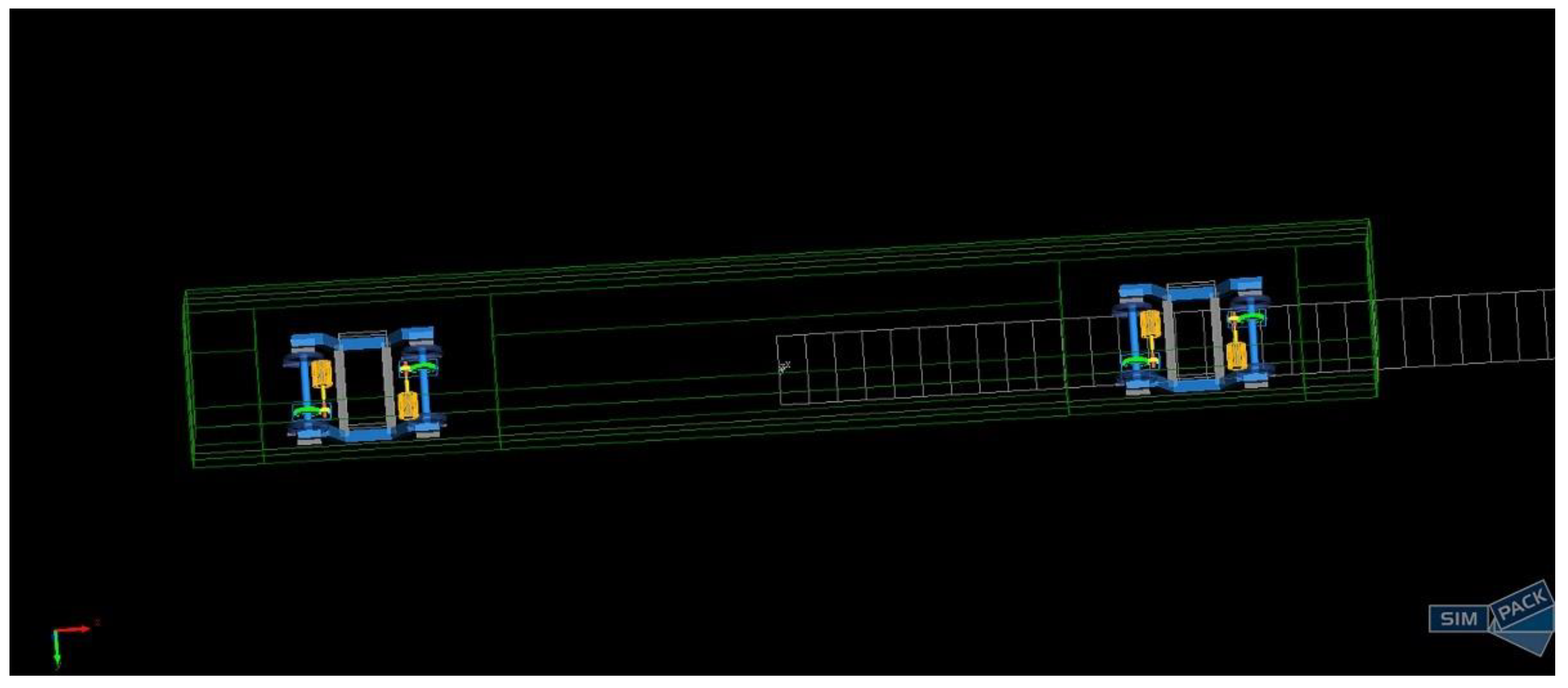
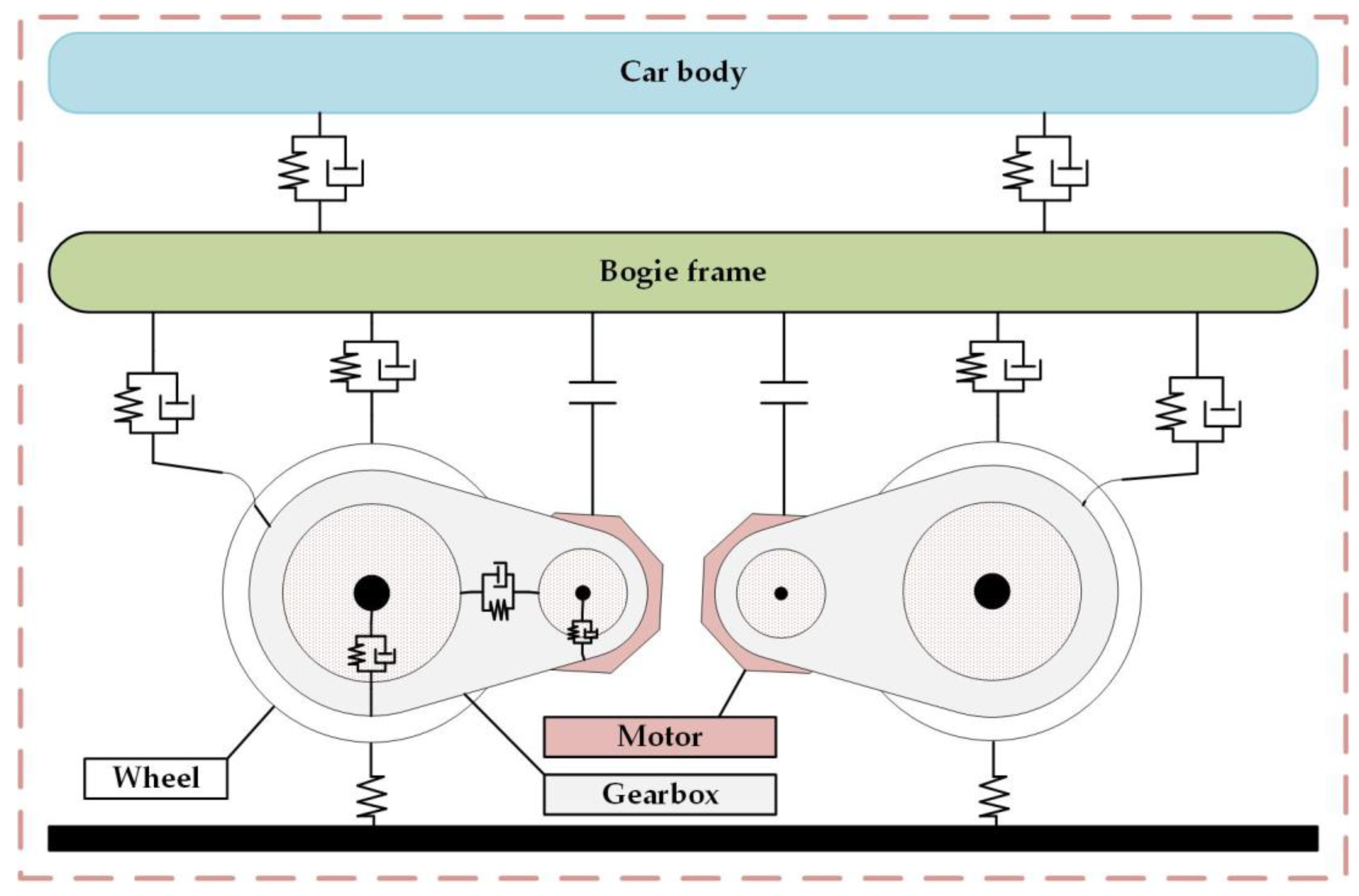
This paper chooses a motor car of the EMU in service as the research object. Figure 1 is the vehicle dynamic model, and Figure 2 is the structural topology of the model. The car body, bogie frame, wheelset, motor, and gearbox are rigid bodies in the dynamic model. The suspension force of both the primary and secondary suspensions consists of parallel springs and damping systems. In addition, the vertical damper of the primary suspension and secondary suspension and the anti-snake movement damper and lateral stops of the secondary suspension are considered nonlinear parameters. The traction motor is fixed to the bogie frame using bolts. The gearbox is connected with the bogie frame through the hanger rod. The transmission system’s rolling bearing and coupling structure is simplified as suspension force with stiffness damping. The gear pair considers the transmission torque and describes the internal excitation factors such as tooth clearance and time-varying meshing stiffness of the gear transmission model. Moreover, the driven gear is fixed to the wheel axle by restraint and maintains synchronous motion.
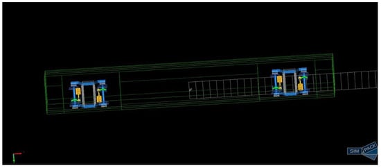
Figure 1.
Top view of the high-speed train dynamics model.
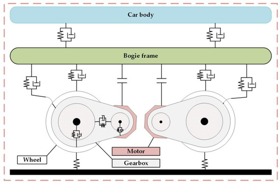
Figure 2.
Topology of vehicle model structure.
In Table 1, the main parameters of cylindrical helical gear transmission in the gearbox model. Moreover, as shown in Table 2, the car body, bogie frame, and wheelset in the vehicle dynamic model have six degrees of freedom relative to the ground. The axle box, gearbox, gear, pinion, and motor rotor have a degree of freedom of rotation around the lateral direction. There are 66 degrees of freedom in the vehicle dynamic model.

Table 1.
Parameters of the gear pair structure.
Table 2.
Degree of freedom of each structure in a vehicle model.
2.2. Electric Model
Due to the complex motion relationship between stator and rotor, the mathematical model of a three-phase induction motor is a strongly coupled nonlinear multivariable system [40]. In order to facilitate the establishment of the motor control system, the linear and decoupled mathematical model is often obtained through coordinate transformation [41,42,43,44,45,46]. In addition, the direct torque control method is often used in large mechanical systems, such as rail vehicles [47,48], because of its natural advantages of quick response and convenience.
2.2.1. Mathematical Model of the Traction Motor
The simplified model of the motor has the following assumptions. First, the three-phase winding is symmetrical. The magnetic force is sinusoidally distributed along the circumference of the air gap. Second, the effect of magnetic saturation, core loss, and temperature and frequency influence on motor resistance is ignored based on the mathematical model theory of asynchronous motor [49]. The mathematical expression of coordinate transformation is usually expressed in matrix equation form as Equation (1):
where A is the transformation matrix, X is the original vector before transformation, and Y is the new vector after transformation.
The above matrix transformation can transform the current matrix in the three static coordinate systems into a new matrix in another coordinate system. Simultaneously, the process satisfies the principle of invariable power before and after transformation.
As shown in Figure 3 below, in the three-phase stationary coordinate system, the A-axis is recombined with the α-axis in the two-phase coordinate system. It is assumed that the adequate number of turns in each phase of the stator winding is N, and the magnetic emf waveform is sinusoidal. The component algebras of the three-phase magnetomotive force on the α and β axes are equal to those of the two-phase magnetomotive force. Equation (2) expresses the relationship as below.
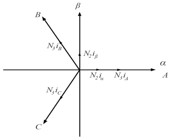
Figure 3.
Schematic diagram of space vector of magnetomotive force.
Equation (3) is the transformation matrix from a three-phase stationary coordinate to a two-phase synchronous coordinate.
Based on the above coordinate system transformation, the mathematical model of asynchronous motor is established in any two-phase coordinate system, and Equations (4) and (5) can express the magnetic flux and voltage equations, respectively:
where the symbols φsd and φsq are the components of stator flux linkage in the two-phase coordinate system, respectively, and φrd and φrq are the components of rotor flux in the two-phase coordinate system; isd, isq, ird, and irq are the components of stator current and rotor current in the two-phase coordinate system, respectively; Ls and Lr are the self-inductance of stator equivalent two-phase windings and rotor equivalent two-phase windings in the two-phase coordinate system, respectively, and Lm is the mutual inductance between coaxial equivalent windings of stator and rotor in the two-phase coordinate system.
where the symbols usd, usq, urd, and urq are components of stator voltage and rotor voltage in the two-phase coordinate system, respectively; Rs and Rr represent the stator resistance and rotor resistance, respectively; p is a differential operator, ωdqs is the angular velocities relative to the stator, and ωdqr is the angular velocity relative to the rotor in the two-phase coordinate system.
According to the kinematics theory [50], the output torque equation of the motor can be expressed by Equation (6), and the motion equation of the motor can be expressed by Equation (7).
where Te is the electromagnetic torque of the motor, np is polar logarithm, Tm is the load torque, J is the moment of inertia of the electromechanical system, and D is the damping coefficient.
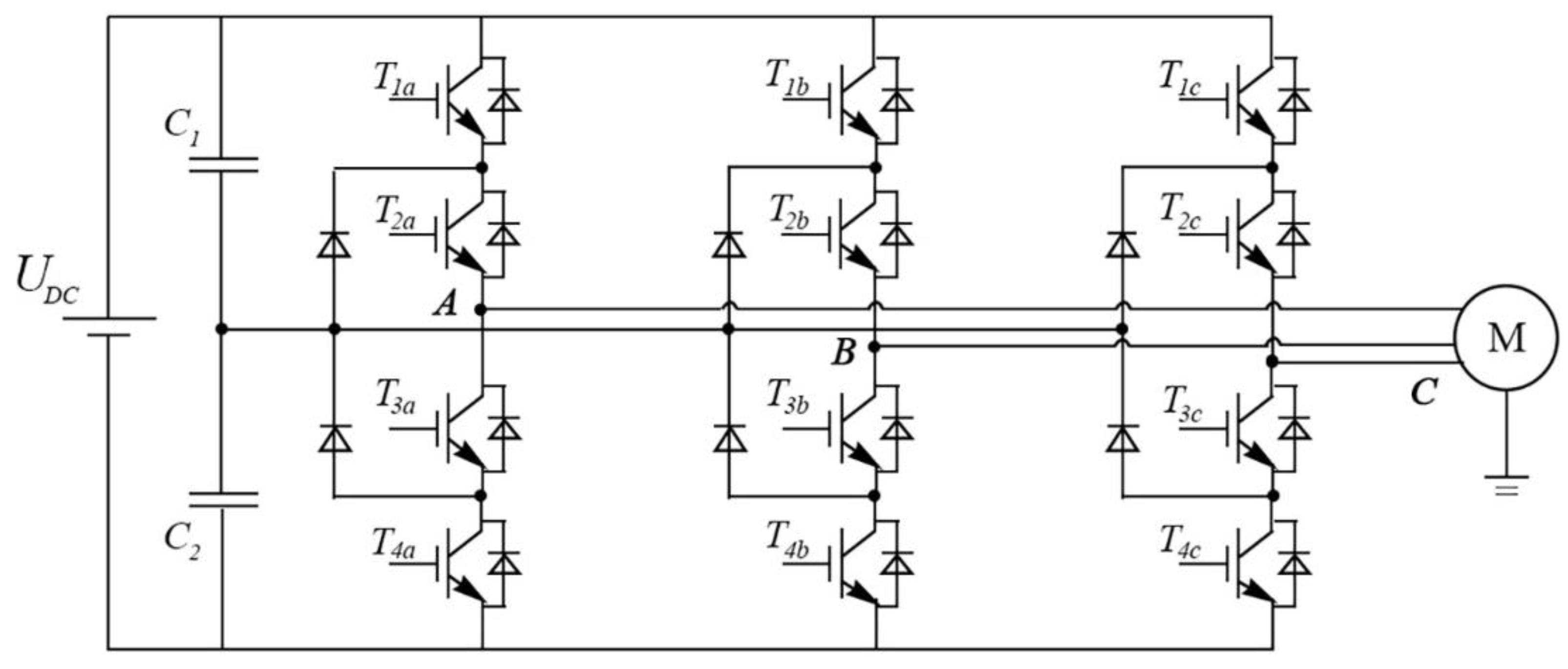
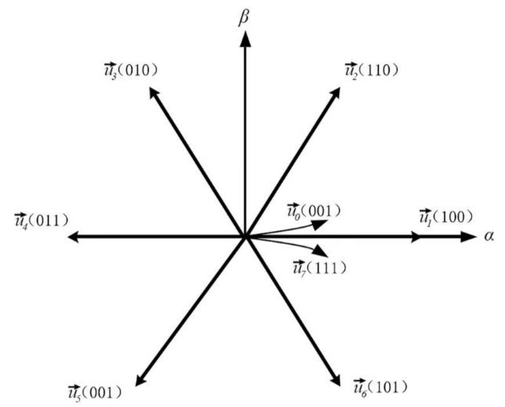
The research in this paper uses a voltage inverter, and Figure 4 shows the schematic diagram of main circuit of traction inverter. The corresponding power grid obtains the dc voltage through the transformer and the rectifier circuit. It outputs the voltage value by switching the inverter to control the motor. If the three-phase load is connected to different phases, the switching state of the inverter is 1. Otherwise, when the three-phase load is connected to the same phase, the switching state of the inverter is 0. Figure 5 is the voltage vector schematic diagram of the inverter. So, there are eight combinations of switching states of inverters, which are as follows: U0 (000), U1 (100), U2 (110), U3 (010), U4 (011), U5 (001), U6 (101), and U7 (111).
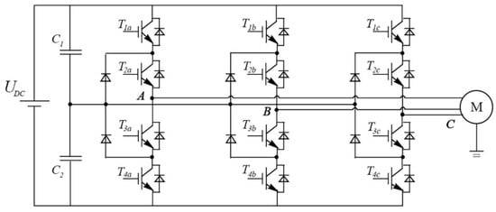
Figure 4.
The main circuit of the thre- level voltage-type traction inverter.

Figure 5.
Schematic diagram of inverter voltage vector.
The eight voltage state-space vectors of the inverter form eight discontinuous voltage space vectors. The angle between the two adjacent vectors in the six non-zero voltage vectors is 60°. The counterclockwise rotation order of the vectors is as follows: U1 → U2 → U3 → U4 → U5 → U6. The stator voltage us in any of the switching states can be expressed as a vector in the two-phase coordinate system.
where uA, uB, and uC are phase voltages of three-phase stator load, respectively.
When the traction motor is connected to the non-sinusoidal power, the time harmonic magneto-motive force will be generated in the air gap of the motor, which will generate additional harmonic torque. When the air gap harmonic flux and harmonic rotor current have the same order, their interaction will produce a stable harmonic torque, and when the times of harmonic flux and harmonic rotor current are different, their interaction will produce a vibration harmonic torque. If the fundamental and harmonic waves in the air gap generate n rotating magnetic fields, there will be (n − 1) stable harmonic torques, and Equation (9) is the calculation formula of kth harmonic torque:
where m is the number of motor stators, np is polar logarithm, f1 is the input fundamental wave voltage frequency of the motor stator, I2k is the calculated value of rotor current under kth harmonics, and Rrk is the rotor resistance calculated to the stator side under kth harmonics.
If the fundamental and harmonic waves in the air gap generate n rotating magnetic fields, there will be (n2 − n) vibration harmonic torques. Equation (10) gives the fifth harmonic vibration torque and Equation (11) gives the 7th harmonic vibration torque.
where E2 is the calculated value of the emf of fundamental rotor, and ϕ2 is the phase difference between current and electromotive force when ωt = 0.
When the train is in traction operation, the pantograph transforms the AC power of cate nary into DC power through high-voltage electrical equipment, a traction transformer and traction converter, and then the traction inverter drives the traction motor by outputting three-phase AC power. During the braking deceleration, the traction inverter is controlled to make the traction motor in the state of power generation, and the traction inverter feeds the three-phase ac power output of the traction motor back to the catenary through the rectification link. As shown in Table 3, we can use A and B to represent the power absorbed and fed back by the traction inverter from the power grid, respectively:
where PM is the output power of traction motor.
Table 3.
Parameter table of traction and the auxiliary inverter.
2.2.2. Asynchronous Motor Control Strategy
This paper uses the direct torque control method to realize the effective control of electromagnetic torque of asynchronous traction motor. The direct torque control method uses magnetic flux and electromagnetic torque as control variables. A discrete inverter vector controls the stator flux vector trajectory. The control method is fast and straightforward, which significantly improves the dynamic response ability of the system.
As shown in Figure 6, the basic flow of the direct torque control method is as follows: The voltage and current signals ua, ub, uc, ia, ib, and ic are sent by the inverter to the asynchronous traction motor are obtained by the measurement module. Then, the components uα, uβ, iα, and iβ of the stator three-phase voltage and current signals after coordinate transformation are obtained by using the Clark transform method [51]. After that, the stator flux and actual torque model are then obtained according to voltage and current components.
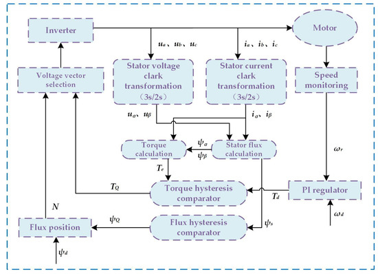
Figure 6.
Principle block diagram of direct torque control for traction motor.
The direct torque control theory [52] shows that the motor stator flux vector and the actual motor torque can be expressed as Equations (13) and (14).
where the symbols ψα and ψβ represent the components of the magnetic vector in a two-phase coordinate system.
Furthermore, the rotational angular velocity ωr of the rotor measured by the speed sensor and the given angular velocity ωd are calculated by P.I. adjustment. As a result, the motor’s reference torque value Te* is obtained. Then, the reference torque value Te* and the actual calculated torque value Te are used to obtain the torque switch signal T.Q. through the hysteresis comparator. Similarly, the flux amplitude ψs obtained by the flux calculation model and the given flux value ψs* can be used to obtain the flux switch signal ψQ by the hysteresis comparator. Meanwhile, the stator flux calculation model determines the interval value N of flux through the S-function. On this basis, the voltage selector switch signal unit is combined with flux interval value N, flow switch signal ψQ, and torque switch signal T.Q. The corresponding voltage switch vector is obtained by the program written by S-function to control the inverter output controllable three-phase A.C. signal.
2.3. Electromechanical Coupling Model
The resistance is an unavoidable external force when the train runs on the line. The running resistance of a high-speed train mainly includes basic resistance and additional resistance. The basic resistance refers to the resistance existing in any operating condition of the train, and the additional resistance refers to the resistance generated by the train in the ramp, curve, tunnel, and other individual working conditions. Therefore, in this paper, the model only considers the influence of the basic resistance, and according to the train traction calculation theory [53,54], its expression is:
where ω is the basic resistance per unit mass, and its unit is N/t; a is the rolling resistance coefficient, which is 8.63 N; b is the swing vibration resistance coefficient, which is 0.07295 N∙h/t; and c is the air resistance coefficient of train operation, which is 0.00112 N∙h/t.
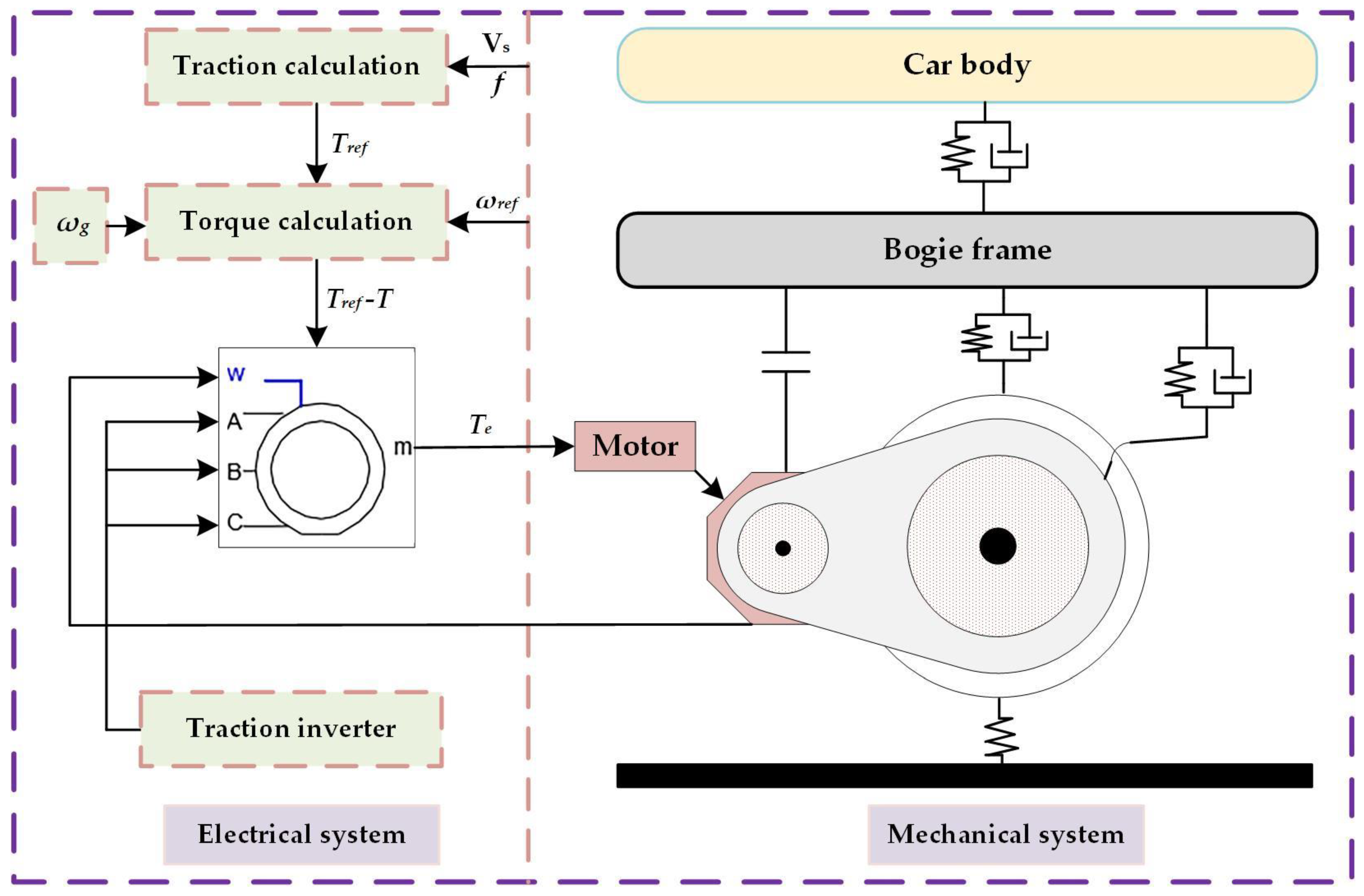
The electromechanical coupling model of a quarter traction drive system is shown in Figure 7. This section describes the coupling process of vehicle mechanical and electrical structures. The co-simulation is between the vehicle dynamic model based on Simpack and the traction motor model based on Simulink by third-party interfaces. The SIMAT interface is realized in the Simpack function module. Firstly, to make the dynamic model normally run in Simulink software, it is necessary to package the dynamic model of the vehicle and set the input and output of the dynamic model. Then, based on the direct torque control method, the torque output of the traction motor is taken as the input of the dynamic model. The real-time angular velocity of the rotor of the vehicle model is the output of the dynamic model and the input value of the traction motor model. Subsequently, the traction motor compares the angular velocity value output by the dynamic model with the given angular velocity value to make a rapid response to control the motor torque output. In addition, the input of the dynamic model uses the basic resistance value calculated from the current running speed of the vehicle model.
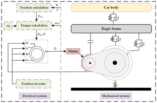
Figure 7.
Electromechanical coupling model of a quarter drive subsystem.
3. Numerical Simulation under Variable Conditions
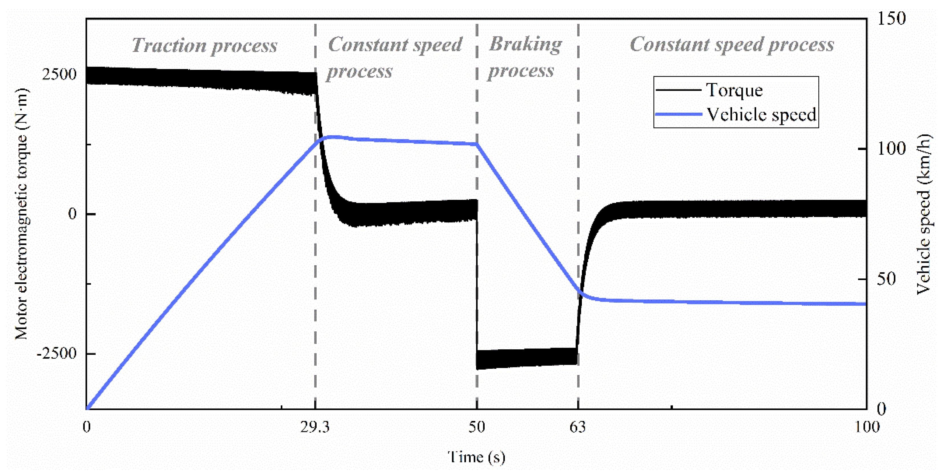
This section describes the specific variable conditions of the simulation. Additionally, the vehicle model simulation in this paper ignores the influence of rail irregularity. First, the vehicle starts to accelerate traction from the initial speed of 0 km/h. During the traction process, the maximum speed of the motor rotor is set to 153 r/s, and the vehicle speed is about 100 km/h at this time. The motor then controls the vehicle to enter the braking process when it travels at a constant speed of 100 km/h for 50 s. Next, in the braking process, the motor speed is set to 60 r/s, and the vehicle running speed is about 40 km/h at this time. Finally, when the rotor speed tends to stabilize, the vehicle runs at a constant speed of 40 km/h for 100 s. Figure 8 below indicates the variation of the motor output torque and vehicle speed.
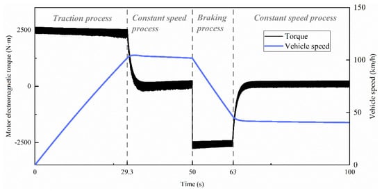
Figure 8.
The variation of motor torque and vehicle speed with time.
In Figure 8, the output torque of the traction motor is about 2500 N∙m in the process of traction acceleration and −2500 N∙m in the braking process. However, the motor’s output torque fluctuates around 0 N∙m in the process of constant speed, and the fluctuation range is about ±150 N∙m. As shown from Figure 8, under the traction acceleration process, the traction motor’s rotor speed accelerates to 153 r/s, and the vehicle accelerates to 100 km/h at the time of 29.3 s. The vehicle then runs at a constant speed for 50 s. After that, the motor outputs the braking torque. Finally, the vehicle enters a stable running state at around 63 s with a motor speed of about 60 r/s (40 km/h for vehicle speed).
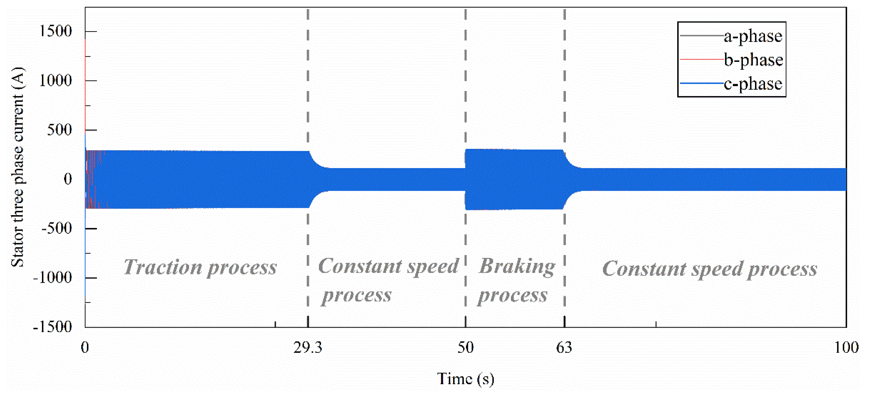
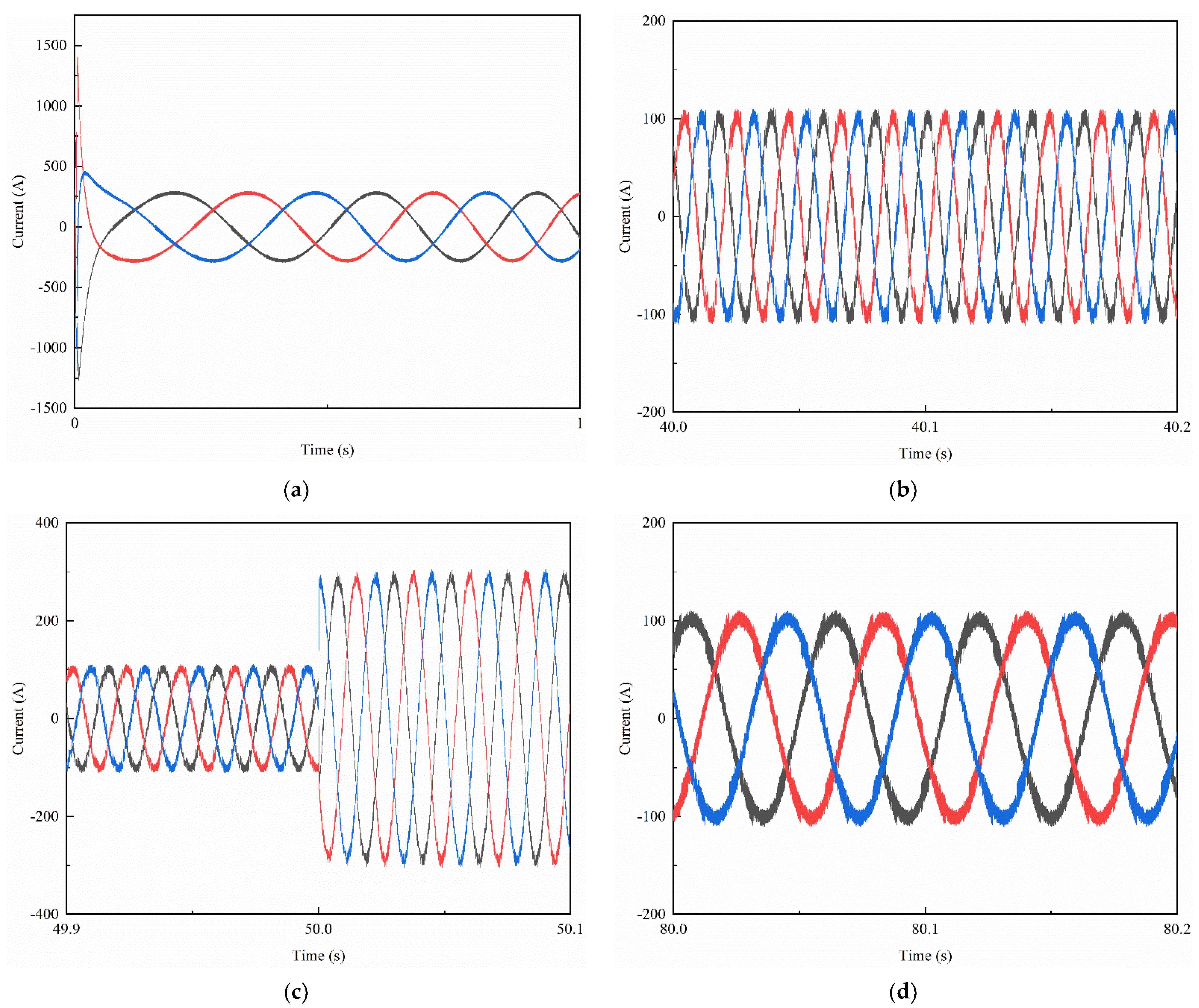
In Figure 9, the stator three-phase current amplitude of the traction motor is prominent in the traction and braking process but small with the constant speed. During the transition from traction acceleration/braking deceleration to constant speed, the current changes relatively gently. It can be seen from Figure 10a that the motor stator current of the vehicle is considerable at the moment of starting. The amplitude reaches about 1400 A. Measures should be taken to avoid damage to the motor caused by the excessive starting current. As shown in Figure 10c, when the vehicle is braking, the three-phase current of the motor stator changes abruptly.
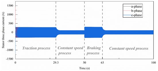
Figure 9.
Time histories of the three-phase current of the motor stator.
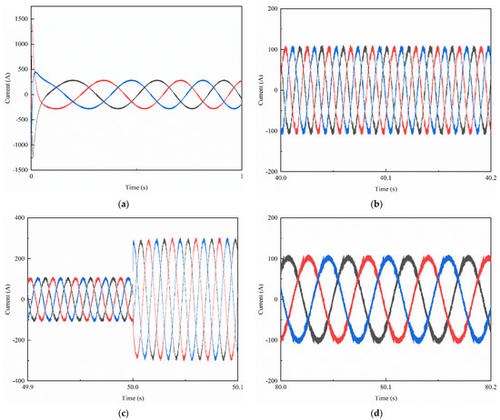
Figure 10.
The stator current in (a) the traction process, (b) the constant speed process at 100 km/h, (c) the braking process, and (d) the constant speed process at 40 km/h.
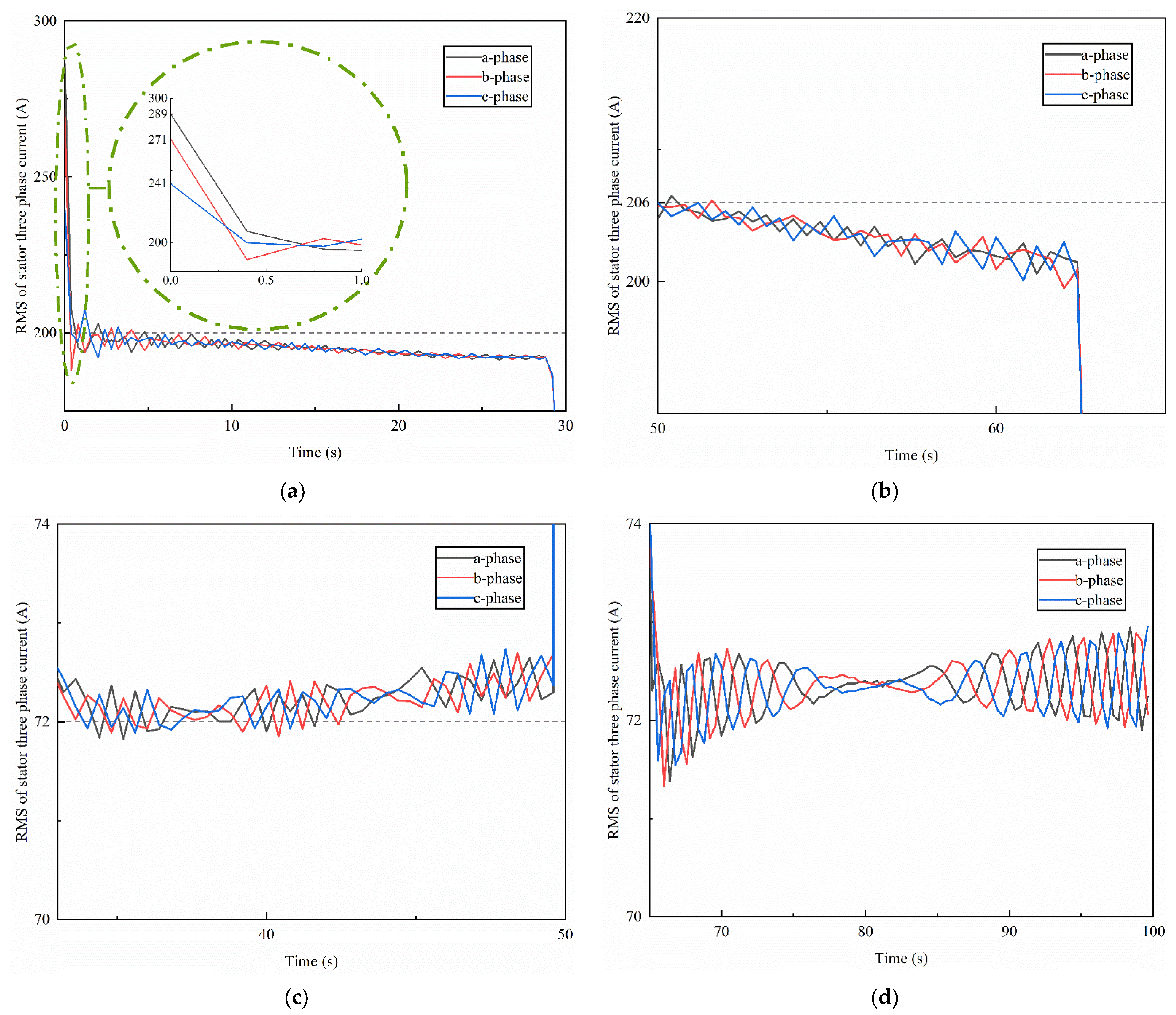
As is shown in Figure 11a, after the vehicle starts, with the increase of the vehicle speed, the RMS of the stator three-phase current of the traction motor decreases gradually from about 200 A in the traction process. Figure 11c shows the braking process, the RMS of the three-phase current of the motor stator is greater than that of the traction process, and the RMS of the current is about 206 A. With the decrease of the vehicle speed, the RMS of the current gradually decreases. In a constant speed process at 100 km/h and 40 km/h, the RMS values vary between 71 A and 73 A.
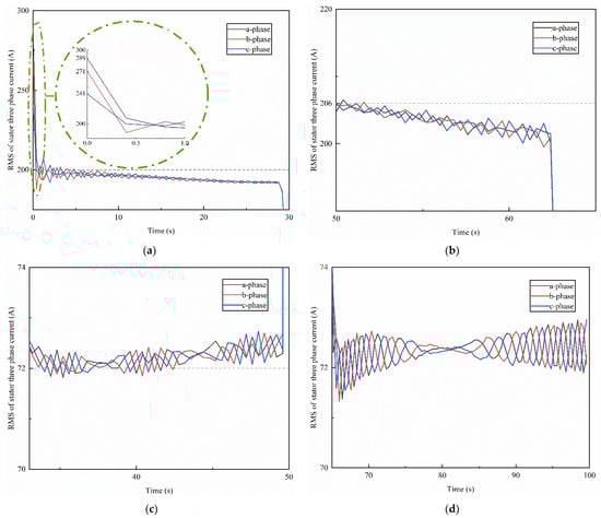
Figure 11.
The RMS value of the stator current in (a) the traction process, (b) the constant speed process at 100 km/h, (c) the braking process, and (d) the constant speed process at 40 km/h.
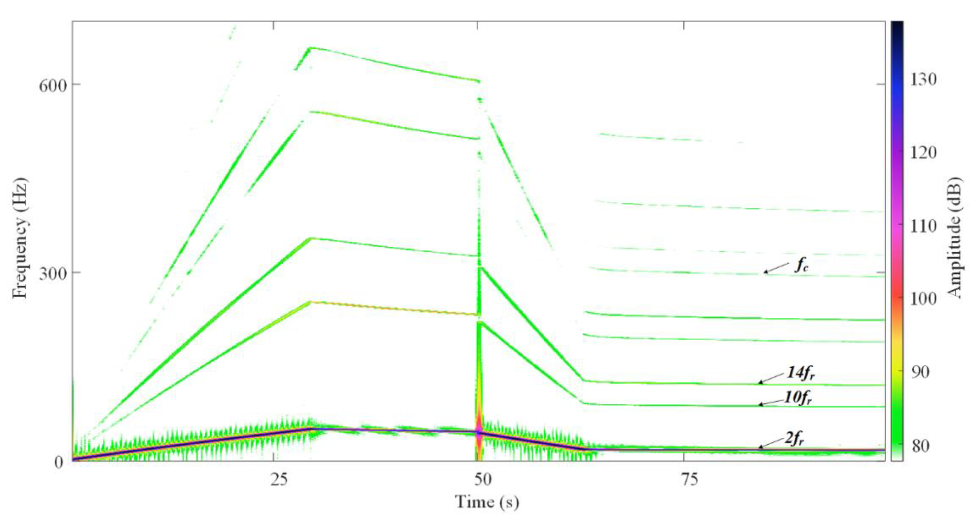
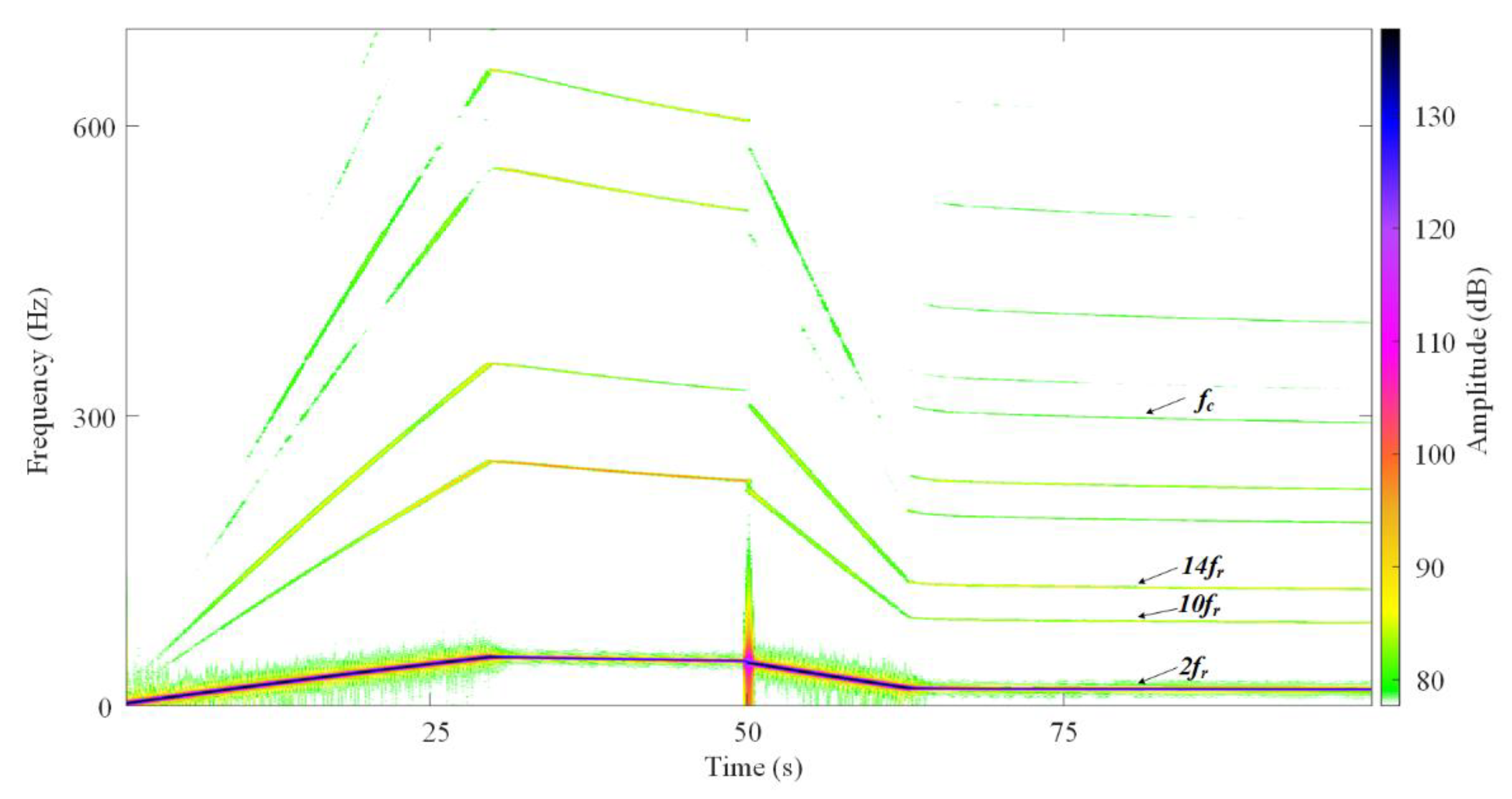
In Figure 12, Figure 13 and Figure 14, the time-frequency analysis of the stator three-phase current indicates that the stator three-phase current frequency gradually rises with the vehicle speed increases. Conversely, the stator three-phase current frequency progressively decreases during the braking process. The theory of the relationship between gear speed and meshing frequency provides the formulas of gear meshing frequency (Equation (16)) and gear shaft rotation frequency (Equation (17)).
where the symbol fc is the meshing frequency of the gear pair, V, N, D, and Z are the vehicle speed, gear teeth, wheel diameter, and pinion teeth, respectively, and fr is the rotation frequency of the pinion shaft.
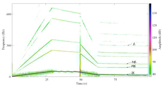
Figure 12.
Time-frequency characteristics of stator three-phase current in a-phase.
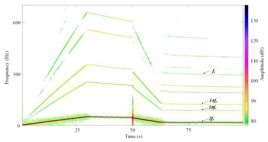
Figure 13.
Time-frequency characteristics of stator three-phase current in b-phase.
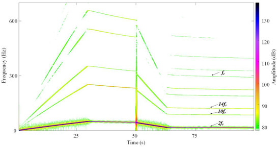
Figure 14.
Time-frequency characteristics of stator three-phase current in c-phase.
When the speed reaches 100 km/h, the stator current frequency is about 49 Hz, and the rotation frequency of the pinion shaft is 24.5 Hz. Furthermore, the stator current frequency is twice the rotational frequency of the pinion shaft. Like the braking process, the stator three-phase current frequency is around 19.5 Hz when the vehicle speed is 40 km/h. Additionally, the rotation frequency of the pinion shaft is 9.8 Hz. It is worth mentioning that the gear meshing frequency fc can also be displayed in the current time-frequency diagram. However, its frequency multiplication is relatively less evident due to the significant meshing frequency of the gear. In addition, harmonic components such as five times and seven times the stator three-phase current can be seen in the time-frequency analysis, mainly due to the control mode of the motor.
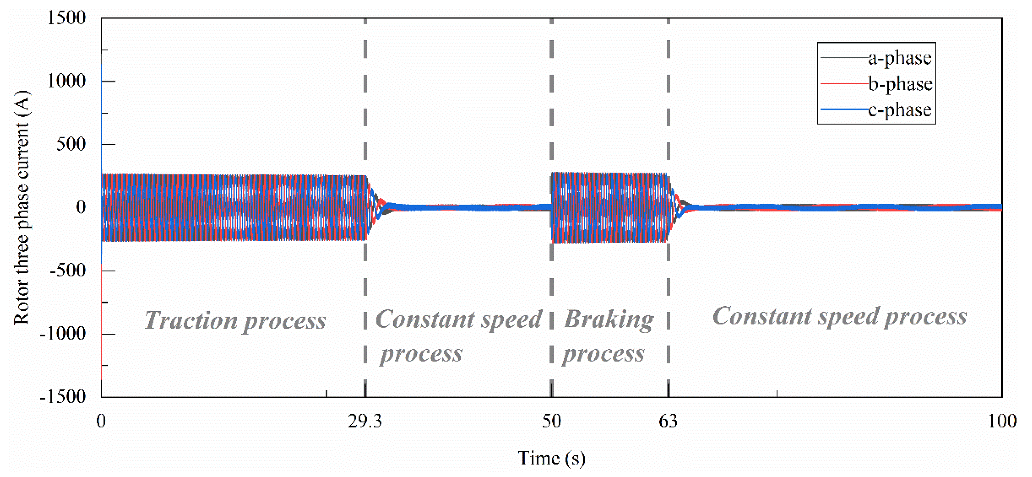
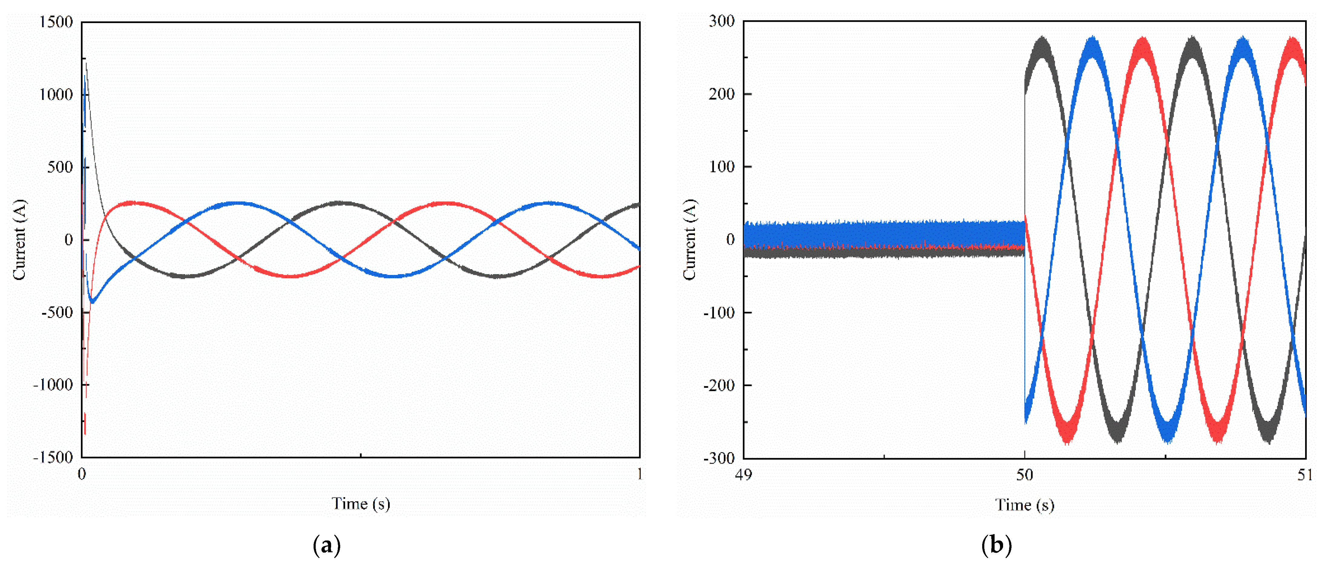
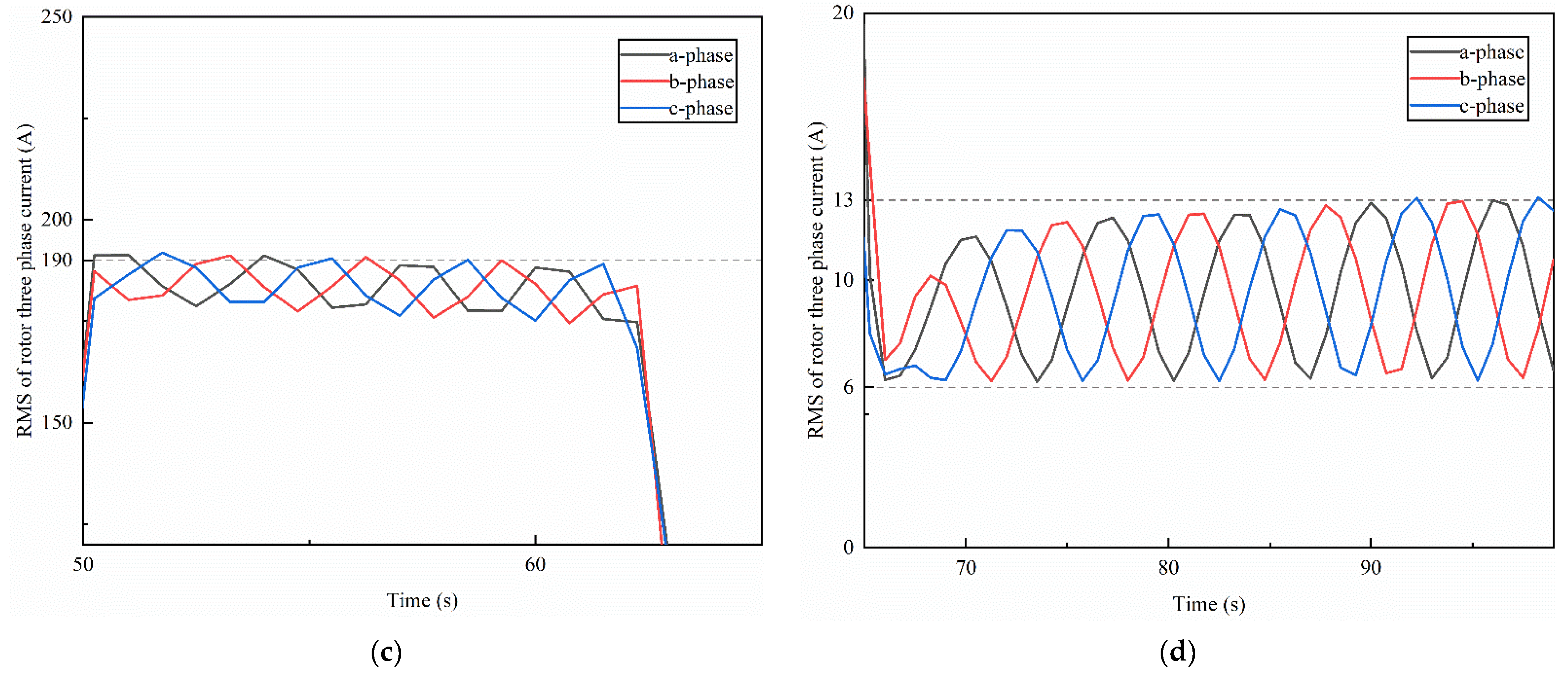
It can be seen from Figure 15 that, at the moment of vehicle starting, the rotor current also has a significant mutation reaching 1250 A, which can be clearly seen in Figure 16a. Compared with the stator three-phase current, the current amplitude decreases significantly from the traction or braking process to the uniform speed process. The rotor three-phase current is relatively stable at a specific value in the uniform speed process. However, the rotor current has a noticeable abrupt change from constant speed to braking. It can be seen from Figure 17a that, in the process of vehicle traction acceleration, the RMS of rotor three-phase current is about 185 A. With the increase of vehicle speed, the RMS value of rotor current tends to decrease. Figure 17c shows that the RMS of rotor current in the braking process is larger than that in the traction process, which is about 190 A and tends to decrease with the vehicle speed. When the vehicle runs at a constant speed of 100 km/h and 40 km/h, the RMS value of the rotor current varies from 6 A to 13 A, which is relatively stable. The rotor current has a more expansive change period and a more minor frequency than the stator current.
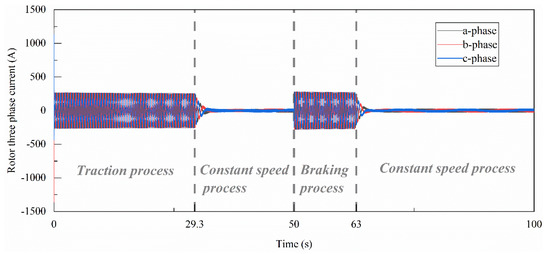
Figure 15.
Time histories of the three-phase current of the motor rotor.
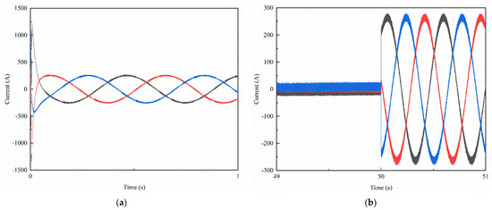
Figure 16.
The variation of rotor current with time at the beginning of (a) the traction process and (b) the braking process.
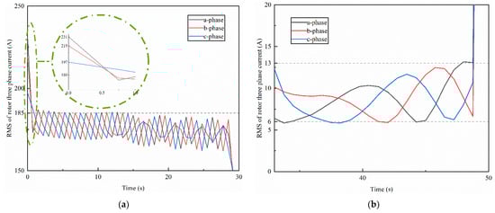
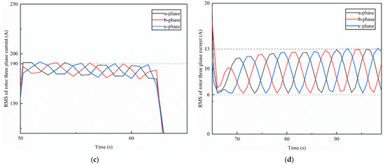
Figure 17.
The RMS value of the rotor current in (a) the traction process, (b) the constant speed process at 100 km/h, (c) the braking process, and (d) the constant process at 40 km/h.
4. Conclusions
This paper established an electromechanical coupling model combined with the traction control and vehicle models. The co-simulation is under traction, constant speed, and braking conditions. Additionally, this research reveals the dynamic characteristics of rotor and stator current during vehicle operation through numerical research. Overall, the conclusions are given as follows.
When the vehicle starts, the current of traction motor stator and rotor have a significant mutation, so measures should be taken to protect the motor. The stator current amplitude reaches 1400 A, and the amplitude of the rotor current reaches 1250 A. The stator current and rotor current gradually decrease with the vehicle speed increase in the traction process. Similarly, the stator current and rotor current decrease gradually with the vehicle speed decrease in the braking process. Both the stator current and rotor current maintain a stable amplitude in the constant speed process.
In order to analyze the change trend of current amplitude of traction motor under the transient condition of variable speed and load, the RMS value is used to describe the change of current amplitude. Similarly, short-time Fourier transform (STFT) is used to analyze the time-frequency characteristics of the current. In the traction and braking process, the RMS value of the stator three-phase current is smaller than that of the braking process. Moreover, the RMS value tends to decrease with the increase or decrease of the vehicle speed during traction and braking. In the traction process, the RMS value of stator current decreases gradually from about 200 A, and while braking, the RMS value of stator current decreases gradually from about 206 A. Moreover, in the constant speed process of 100 km/h and 40 km/h, the RMS value varies between 71 A and 73 A, respectively. The high harmonic of driving shaft rotation frequency and the frequency of gear meshing can be seen in the stator current spectrum. At the vehicle speed of 100 km/h, the stator current frequency (about 49 Hz) is twice as high as the pinion shaft rotation frequency (about 24.5 Hz). The same pattern is observed at a speed of 40 km/h. Except for the rotational frequencies at two constant speeds, these higher harmonics are evident and obscure during the traction and braking process.
In the traction process, the RMS value of the rotor three-phase current is smaller than that of braking. Therefore, during the traction process and braking process, the RMS value of the current all tends to decrease gradually. In the traction process, the RMS value of the rotor current decreases gradually from about 185 A, and while braking, the RMS value of rotor current decreases gradually from about 190 A. The RMS value of the rotor current fluctuates stably in the range of 6 A to 13 A during constant speed. However, it tends to decrease during the traction and braking process.
Author Contributions
Conceptualization, K.Z., J.Y., C.L., J.W. and D.Y.; methodology, K.Z., J.Y. and J.W.; software, K.Z. and J.W.; validation, K.Z., J.Y., C.L., J.W. and D.Y.; formal analysis, K.Z., J.Y. and J.W.; investigation, K.Z. and J.Y.; resources, J.Y., C.L., J.W. and D.Y.; data curation, K.Z., J.Y. and J.W.; writing—original draft preparation, K.Z.; writing—review and editing, K.Z.; visualization, K.Z.; supervision, J.Y., C.L., J.W. and D.Y.; project administration, J.Y., C.L., J.W. and D.Y.; funding acquisition, J.Y., C.L., J.W. and D.Y. All authors have read and agreed to the published version of the manuscript.
Funding
This paper was supported by the National Natural Science Foundation of China (grant number 51975038), the Beijing Natural Science Foundation (grant number 3214042, KZ202010016025, L191005), the Beijing Postdoctoral Research Foundation (grant number 2021-zz-114), the Open Research Fund Program of Beijing Key Laboratory of Performance Guarantee on Urban Rail Transit Vehicles (grant number PGU2020K001), the Fundamental Research Funds for the Beijing Universities (grant number X21049), and the Development of High-Level Teachers in Beijing Municipal Universities (grant number CIT&TCD201904062).
Institutional Review Board Statement
Not applicable.
Informed Consent Statement
Not applicable.
Data Availability Statement
Not applicable.
Conflicts of Interest
The authors declare no conflict of interest.
References
- Feng, J.H.; Wang, J.; Li, J.H. Integrated Simulation Platform of High-Speed Train Traction Drive System. Tiedao Xuebao/J. China Railw. Soc. 2012, 34, 21–26. [Google Scholar]
- Chen, Z.G.; Shao, Y.M.; Lim, T.C. Non-Linear Dynamic Simulation of Gear Response under the Idling Condition. Int. J. Autom. Technol. 2012, 13, 541–552. [Google Scholar] [CrossRef]
- Shantarenko, S.; Kuznetsov, V.; Ponomarev, E.; Vaganov, A.; Evseev, A. Influence of Process Parameters on Dynamics of Traction Motor Armature. Transp. Res. Proced. 2021, 54, 961–971. [Google Scholar] [CrossRef]
- Wang, Z.; Mei, G.; Zhang, W.; Cheng, Y.; Zou, H.; Huang, G. Effects of Polygonal Wear of Wheels on the Dynamic Performance of the Gearbox Housing of a High-Speed Train. Proc. Inst. Mech. Eng. Part F J. Rail Rapid Transit 2018, 232, 095440971775299. [Google Scholar] [CrossRef]
- Wang, Z.; Cheng, Y.; Mei, G.; Zhang, W.; Huang, G.; Yin, Z. Torsional Vibration Analysis of the Gear Transmission System of High-Speed Trains with Wheel Defects. Proc. Inst. Mech. Eng. Part F J. Rail Rapid Transit 2019, 234, 095440971983379. [Google Scholar] [CrossRef]
- Henao, H.; Kia, S.H.; Capolino, G.A. Torsional-Vibration Assessment and Gear-Fault Diagnosis in Railway Traction System. IEEE Trans. Ind. Electron. 2011, 58, 1707–1717. [Google Scholar] [CrossRef]
- Garg, V.K.; Dukkipati, R.V. Dynamics of Railway Vehicle Systems; Academic Press: Cambridge, MA, USA, 1984; pp. 245–247. [Google Scholar]
- Zhai, W. The Vertical Model of Vehicle-Track System and Its Coupling Dynamics. J. China Railw. Soc. 1992, 14, 10–21. [Google Scholar]
- Ren, Z.S.; Zhai, W.M.; Wang, Q.C. Study on Lateral Dynamic Characteristics of Vehicle Turnout System. J. China Railw. Soc. 2000, 22, 28–33. [Google Scholar] [CrossRef]
- Nielsen, J.; Igeland, A. Vertical Dynamic Interaction between Train and Track Influence of Wheel and Track Imperfections. J. Sound Vib. 1995, 187, 825–839. [Google Scholar] [CrossRef]
- Zhai, W.M.; Wang, K.Y. Lateral Interactions of Trains and Tracks on Small-Radius Curves: Simulation and Experiment. Veh. Syst. Dyn. 2006, 44 (Suppl. S1), 520–530. [Google Scholar] [CrossRef]
- Wang, J.; Yang, J.; Zhao, Y.; Bai, Y.; He, Y. Nonsmooth Dynamics of a Gear-Wheelset System of Railway Vehicles under Traction/Braking Conditions. J. Comput. Nonlinear Dyn. 2020, 15, 081003. [Google Scholar] [CrossRef]
- Wang, J.; Yang, J.; Li, Q. Quasi-Static Analysis of the Nonlinear Behavior of a Railway Vehicle Gear System Considering Time-Varying and Stochastic Excitation. Nonlinear Dyn. 2018, 93, 463–485. [Google Scholar] [CrossRef]
- Huang, G.H.; Zhou, N.; Zhang, W.H. Effect of Internal Dynamic Excitation of the Traction System on the Dynamic Behavior of a High-Speed Train. Proc. Inst. Mech. Eng. Part F J. Rail Rapid Transit 2016, 230, 0954409715617787. [Google Scholar] [CrossRef]
- Zhang, W.H.; Shen, Z.Y.; Zeng, J. Study on Dynamics of Coupled Systems in High-Speed Trains. Veh. Syst. Dyn. Int. J. Veh. Mech. Mobil. 2013, 51, 966–1016. [Google Scholar] [CrossRef]
- Yao, Y.; Zhang, H.J.; Luo, S.H. Analysis on Resonance of Locomotive Drive System under Wheel-Rail Saturated Adhesion. J. China Railw. Soc. 2011, 33, 16–22. [Google Scholar]
- Yao, Y.; Zhang, H.J.; Luo, S.H. An Analysis of Resonance Effects in Locomotive Drive Systems Experiencing Wheel/Rail Saturation Adhesion. Proc. Inst. Mech. Eng. Part F J. Rail Rapid Transit 2014, 228, 4–15. [Google Scholar] [CrossRef]
- Farshidianfar, A.; Saghafi, A. Global Bifurcation and Chaos Analysis in Nonlinear Vibration of Spur Gear Systems. Nonlinear Dyn. 2014, 75, 783–806. [Google Scholar] [CrossRef]
- Chen, Z.; Zhou, Z.; Zhai, W.; Wang, K. Improved Analytical Calculation Model of Spur Gear Mesh Excitations with Tooth Profile Deviations. Mech. Mach. Theory 2020, 149, 103838. [Google Scholar] [CrossRef]
- Chen, Z.; Zhai, W.; Wang, K. Vibration Feature Evolution of Locomotive with Tooth Root Crack Propagation of Gear Transmission System. Mech. Syst. Signal Process. 2019, 115, 29–44. [Google Scholar] [CrossRef]
- Chen, Z.; Zhu, Z.; Shao, Y. Fault Feature Analysis of Planetary Gear System with Tooth Root Crack and Flexible Ring Gear Rim. Eng. Fail. Anal. 2015, 49, 92–103. [Google Scholar] [CrossRef]
- Chen, Z.; Zhai, W.; Wang, K. Dynamic Investigation of a Locomotive with Effect of Gear Transmissions under Tractive Conditions. J. Sound Vib. 2017, 408, 220–233. [Google Scholar] [CrossRef]
- Wang, J.; Yang, J.; Lin, Y.; He, Y. Analytical Investigation of Profile Shifts on the Mesh Stiffness and Dynamic Characteristics of Spur Gears. Mech. Mach. Theory 2022, 167, 104529. [Google Scholar] [CrossRef]
- Wang, J.; Yang, J.; Bai, Y.; Zhao, Y.; Yao, D. A Comparative Study of the Vibration Characteristics of Railway Vehicle Axlebox Bearings with Inner/Outer Race Faults. Proc. Inst. Mech. Eng. Part F J. Rail Rapid Transit 2020, 235, 1–13. [Google Scholar] [CrossRef]
- Liu, P.F.; Zhai, W.M.; Wang, K.Y. Establishment and Verification of Three-Dimensional Dynamic Model for Heavy-Haul Train–Track Coupled System. Veh. Syst. Dyn. 2016, 54, 1511–1537. [Google Scholar] [CrossRef]
- Liu, Y.; Chen, Z.; Tang, L.; Zhai, W. Skidding Dynamic Performance of Rolling Bearing with Cage Flexibility under Accelerating Conditions. Mech. Syst. Signal Process. 2021, 150, 107257. [Google Scholar] [CrossRef]
- Park, S.; Kim, W.; Kim, S.I. A Numerical Prediction Model for Vibration and Noise of Axial Flux Motors. IEEE Trans. Ind. Electron. 2014, 61, 5757–5762. [Google Scholar] [CrossRef]
- Qi, Y.; Dai, H. Influence of Motor Harmonic Torque on Wheel Wear in High-Speed Trains. Proc. Inst. Mech. Eng. Part F J. Rail Rapid Transit 2019, 234, 095440971983080. [Google Scholar] [CrossRef]
- Guasch-Pesquer, L.; Youb, L.; González-Molina, F.; Zeppa-Durigutti, E. Effects of Voltage Unbalance on Torque and Current of the Induction Motors. In Proceedings of the IEEE 2012 13th International Conference on Optimization of Electrical and Electronic Equipment (OPTIM), Brasov, Romania, 24–26 May 2012. [Google Scholar]
- Pustovetov, M.Y.; Pustovetov, K.M. The Electromagnetic Torque Ripple of Three-Phase Induction Electric Machine, Operating as a Part of the Auxiliary Electric Drive Onboard of A.C. Electric Locomotive—A Factor Contributing to the Failure of Bearings. In Proceedings of the IEEE 2018 International Multi-Conference on Industrial Engineering and Modern Technologies (FarEastCon), Vladivostok, Russia, 3–4 October 2018. [Google Scholar]
- Wang, Z.; Wang, R.; Crosbee, D.; Allen, P.; Zhang, W. Wheel Wear Analysis of Motor and Unpowered Car of a High-Speed Train. Wear 2019, 444–445, 203136. [Google Scholar] [CrossRef]
- Wang, Z.W.; Mei, G.M.; Xiong, Q.; Yin, Z.H.; Zhang, W.H. Motor Car-Track Spatial Coupled Dynamics Model of a High-Speed Train with Traction Transmission Systems. Mech. Mach. Theory 2019, 137, 386–403. [Google Scholar] [CrossRef]
- Wu, P.B.; Guo, J.Y.; Wu, H.; Wei, J. Influence of DC-Link Voltage Pulsation of Transmission Systems on Mechanical Structure Vibration and Fatigue in High-Speed Trains. Eng. Fail. Anal. 2021, 130, 105772. [Google Scholar] [CrossRef]
- Zhu, H.Y.; Yin, B.C.; Hu, H.T.; Xiao, Q. Effects of Harmonic Torque on Vibration Characteristics of Gear Box Housing and Traction Motor of High-Speed Train. J. Traffic Transp. Eng. 2019, 19, 65–76. (In Chinese) [Google Scholar]
- Li, G.L. Research on Harmonic Suppression of Urban Rail Transit Traction Motor Based on Proportional Resonant Regulator. Railw. Locomot. Car 2019, 39, 111–115. (In Chinese) [Google Scholar]
- Li, G.Q.; Liu, Z.M.; Guo, R.B. Stress Response and Fatigue Damage Assessment of High-Speed Train Gearbox. J. Traffic Transp. Eng. 2018, 18, 79–88. (In Chinese) [Google Scholar]
- Liang, X.R.; Xiao, L.; Wang, X.Q. Design of Neural Network PID Controller for Speed Tracking of High-Speed Train. Comput. Eng. Appl. 2021, 57, 252–258. (In Chinese) [Google Scholar]
- Xu, C.F.; Chen, X.Y.; Zheng, X. Slip Velocity Tracking Control of High-speed Train Using Dynamic Surface Method. J. Railw. 2020, 42, 41–49. (In Chinese) [Google Scholar]
- Hou, T.; Guo, Y.Y.; Chen, Y. Study on Speed Control of High-Speed Train Based Multi-Point Model. J. Railw. Sci. Eng. 2020, 17, 314–325. (In Chinese) [Google Scholar]
- Takahashi, I.; Noguchi, T. A New Quick-Response and High-Efficiency Control Strategy of an Induction Motor. IEEE Trans. Ind. Appl. 1986, 22, 820–827. [Google Scholar] [CrossRef]
- Zhang, Z.; Tang, R.; Bai, B.; Xie, D. Novel Direct Torque Control Based on Space Vector Modulation with Adaptive Stator Flux Observer for Induction Motors. IEEE Trans. Magn. 2010, 46, 3133–3136. [Google Scholar] [CrossRef]
- Habetler, T.G.; Profumo, F.; Pastorelli, M. Direct Torque Control of Induction Machines Using Space Vector Modulation. Ind. Appl. IEEE Trans. 1992, 28, 1045–1053. [Google Scholar] [CrossRef]
- Jin, S.; Li, M.; Zhu, L.; Liu, G.; Zhang, Y. Direct Torque Control of Open Winding Brushless Doubly-Fed Machine. In Proceedings of the 2017 IEEE International Magnetics Conference (INTERMAG), Dublin, Ireland, 24–28 April 2017. [Google Scholar]
- Casadei, D.; Serra, G.; Tani, K. Implementation of a Direct Control Algorithm for Induction Motors Based on Discrete Space Vector Modulation. Power Electron. IEEE Trans. 2000, 15, 769–777. [Google Scholar] [CrossRef]
- Beerten, J.; Verveckken, J.; Driesen, J. Predictive Direct Torque Control for Flux and Torque Ripple Reduction. IEEE Trans. Ind. Electron. 2010, 57, 404–412. [Google Scholar] [CrossRef]
- Stojic, D.; Milinkovic, M.; Veinovic, S.; Klasnic, I. Improved Stator Flux Estimator for Speed Sensorless Induction Motor Drives. Power Electron. IEEE Trans. 2014, 30, 2363–2371. [Google Scholar] [CrossRef]
- Buja, G.S.; Kazmierkowski, M.P. Direct Torque Control of PWM Inverter-Fed AC Motors—A Survey. IEEE Trans. Ind. Electron. 2004, 51, 744–757. [Google Scholar] [CrossRef]
- Demir, R.; Barut, M.; Yildiz, R.; Inan, R.; Zerdali, E. EKF Based Rotor and Stator Resistance Estimations for Direct Torque Control of Induction Motors. In Proceedings of the 2017 International Conference on Optimization of Electrical and Electronic Equipment (OPTIM) & 2017 Intl Aegean Conference on Electrical Machines and Power Electronics (ACEMP), Brasov, Romania, 25–27 May 2017. [Google Scholar]
- Barnes, M. Practical Variable Speed Drives and Power Electronics. Pract. Variab. Speed Drives Power Electron. 2003, 4, 156–177. [Google Scholar]
- Faiz, J.; Hossieni, S.H.; Ghaneei, M. Direct Torque Control of Induction Motors for Electric Propulsion System. Electr. Power Syst. Res. 1999, 51, 95–101. [Google Scholar] [CrossRef]
- Vaez-Zadeh, S.; Jalali, E. Combined Vector Control and Direct Torque Control Method for High Performance Induction Motor Drives. Energy Convers. Manag. 2007, 48, 3095–3101. [Google Scholar] [CrossRef]
- Baader, U.; Depenbrock, M.; Gierse, G. Direct Self Control of Inverter-Fed Induction Machine, a Basis for Speed Control without Speed-Measurement. In Proceedings of the Conference Record of the IEEE Industry Applications Society Annual Meeting, San Diego, CA, USA, 1–5 October 1989. [Google Scholar]
- Rao, Z. Calculation of Train Traction; China Railway Press: Beijing, China, 1997. (In Chinese) [Google Scholar]
- Wen, X.Y. Research on Traction Motor Optimization Control for Low Speed Operation of Locomotive; Beijing Jiaotong University: Beijing, China, 2012. (In Chinese) [Google Scholar]


Publisher’s Note: MDPI stays neutral with regard to jurisdictional claims in published maps and institutional affiliations. |
© 2022 by the authors. Licensee MDPI, Basel, Switzerland. This article is an open access article distributed under the terms and conditions of the Creative Commons Attribution (CC BY) license (https://creativecommons.org/licenses/by/4.0/).