
A Demand Response Implementation with Building Energy Management System


Abstract
:1. Introduction
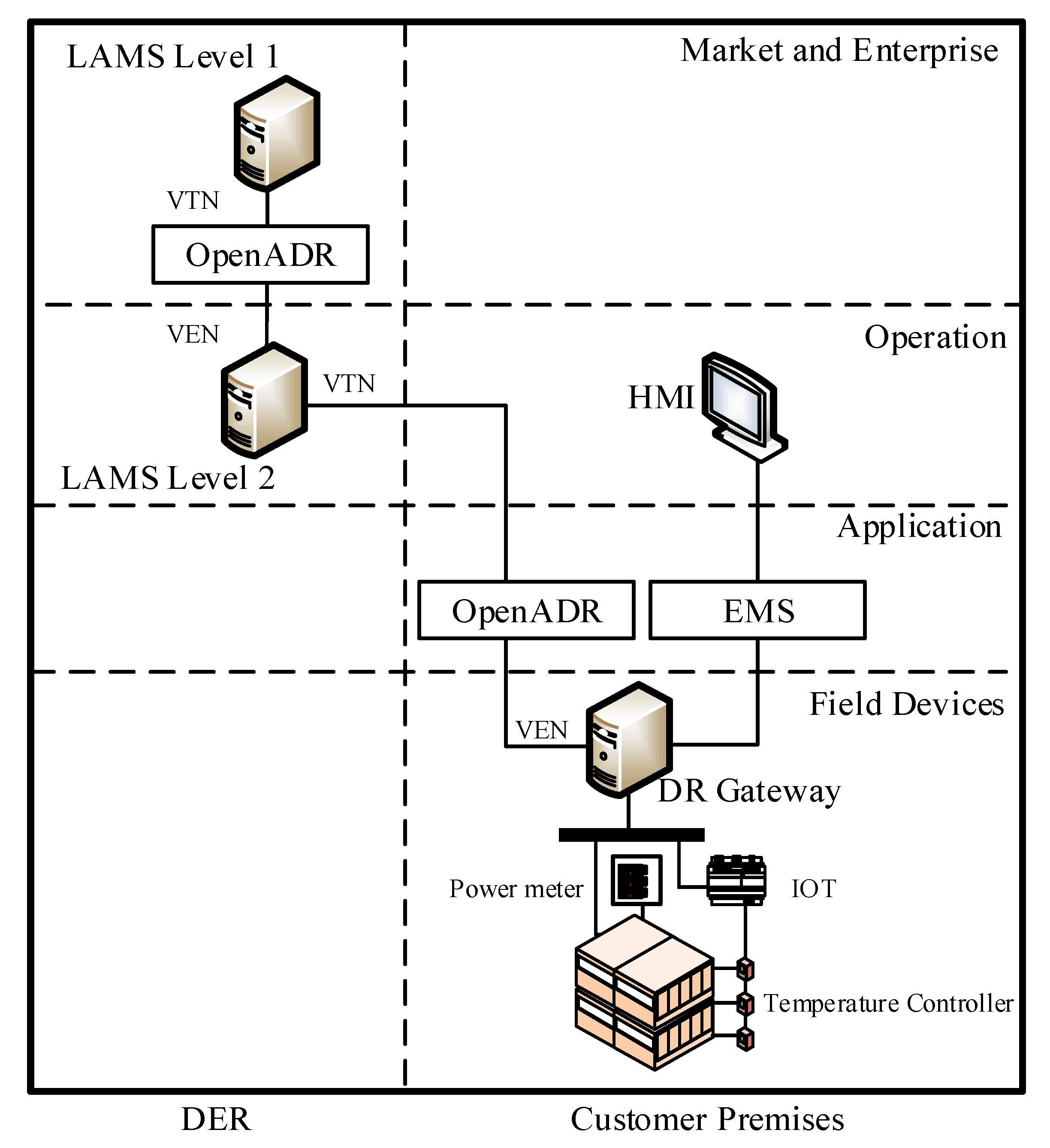
2. System Overview
2.1. System Design
2.1.1. The Market Layer
2.1.2. The Operation Layer
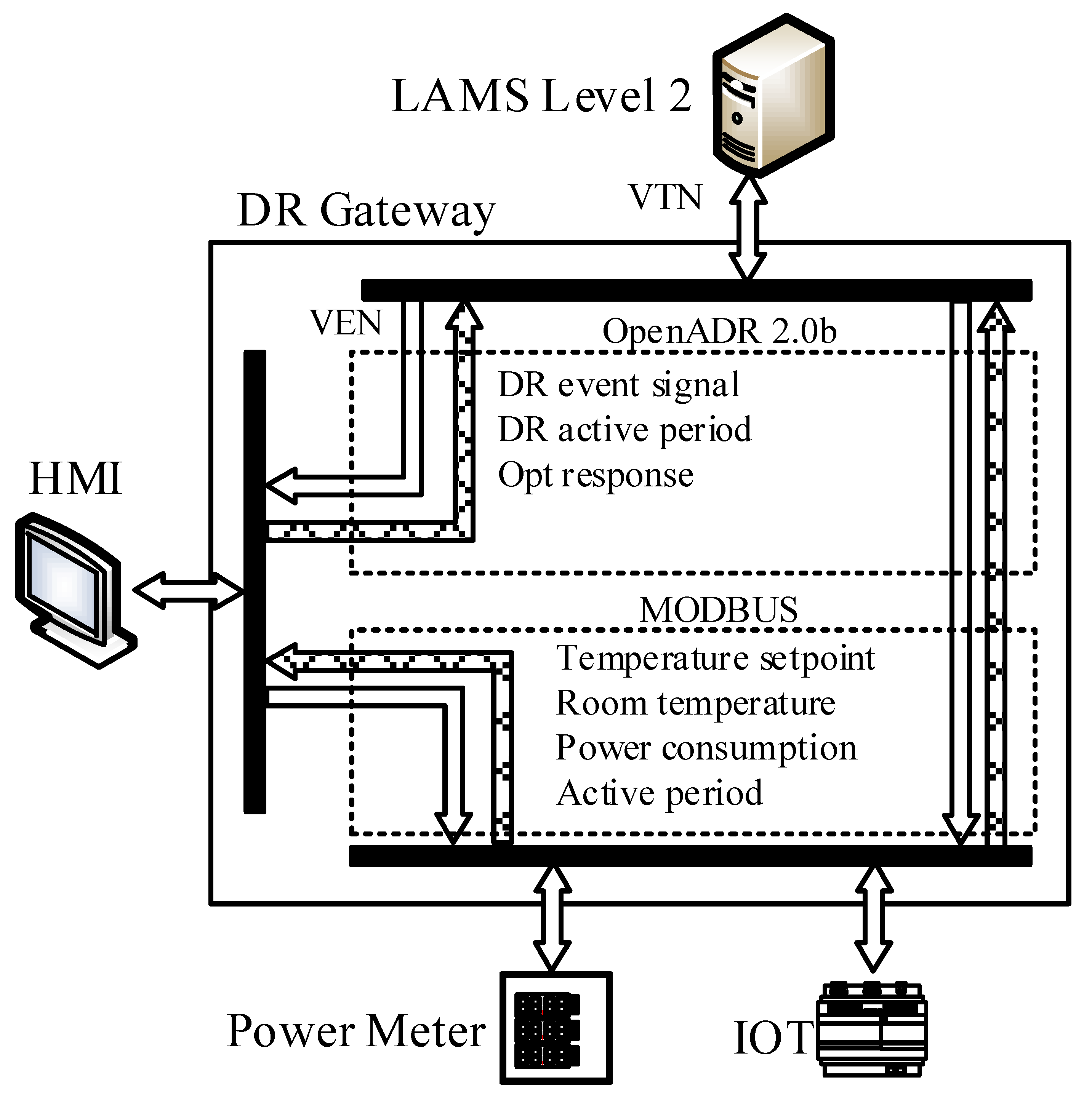
2.1.3. The Application Layer
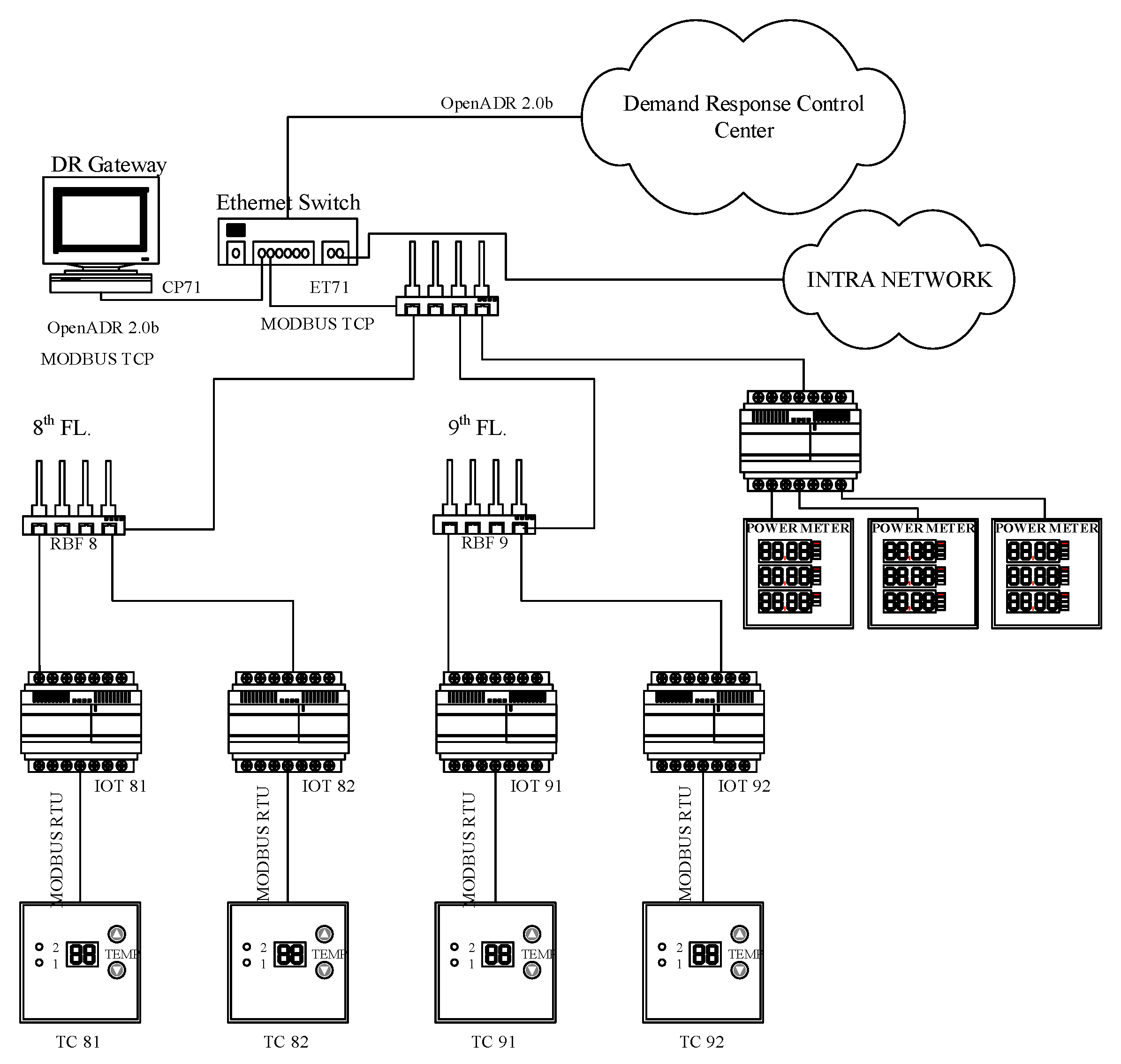
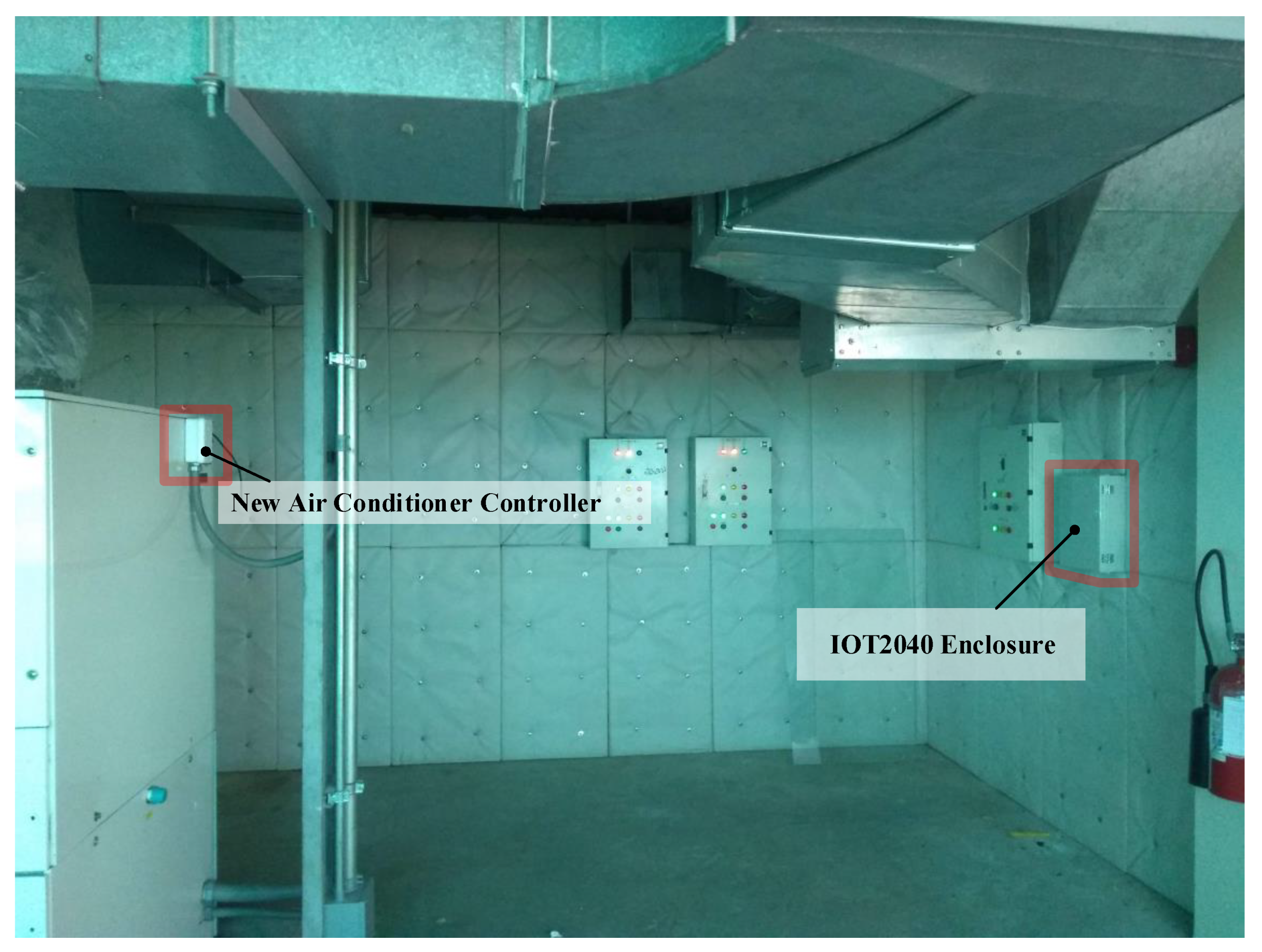
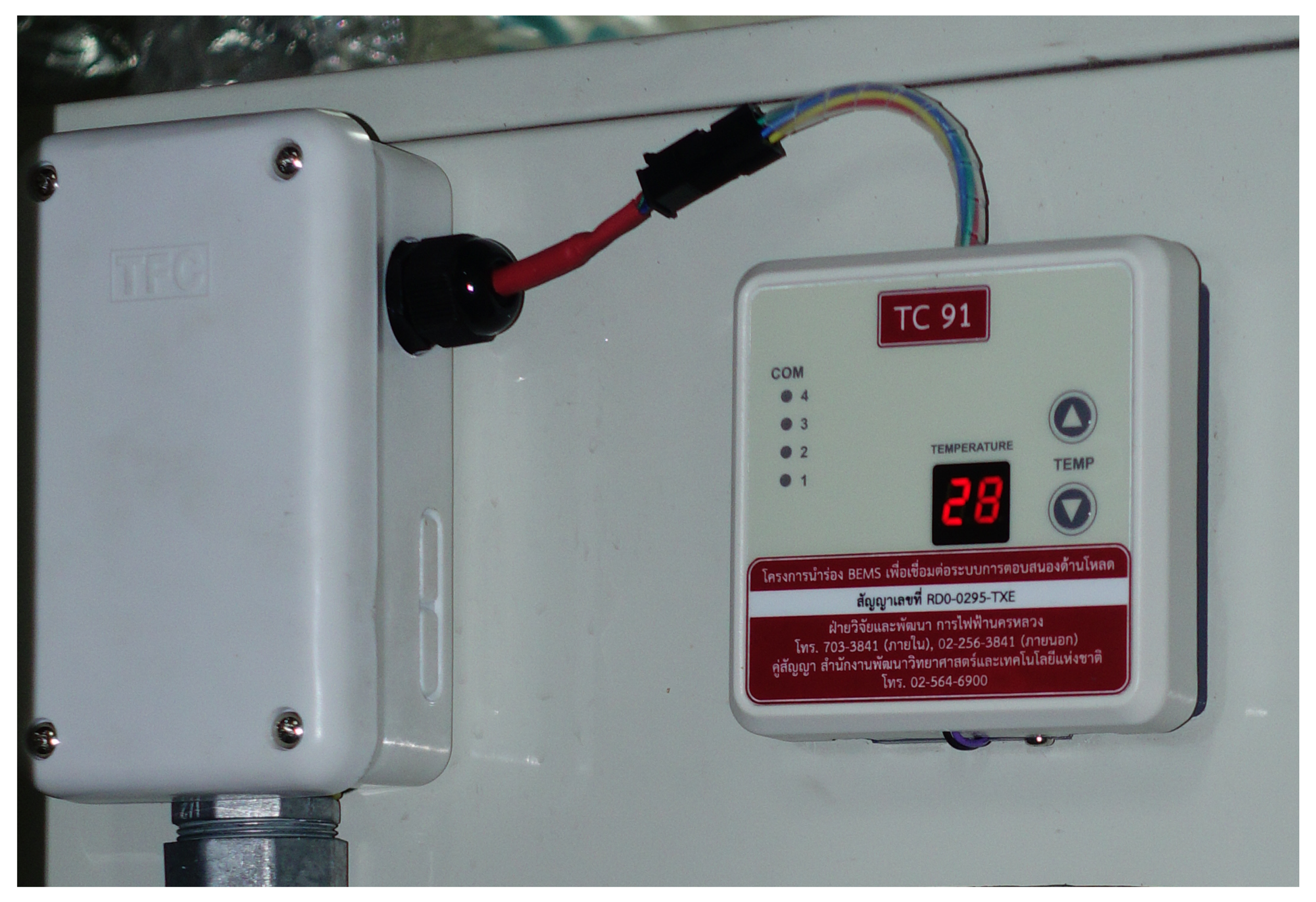
2.1.4. The Field Devices Layer
2.2. Building Characteristics
2.2.1. Site Location
2.2.2. Typical Energy Consumption Profile
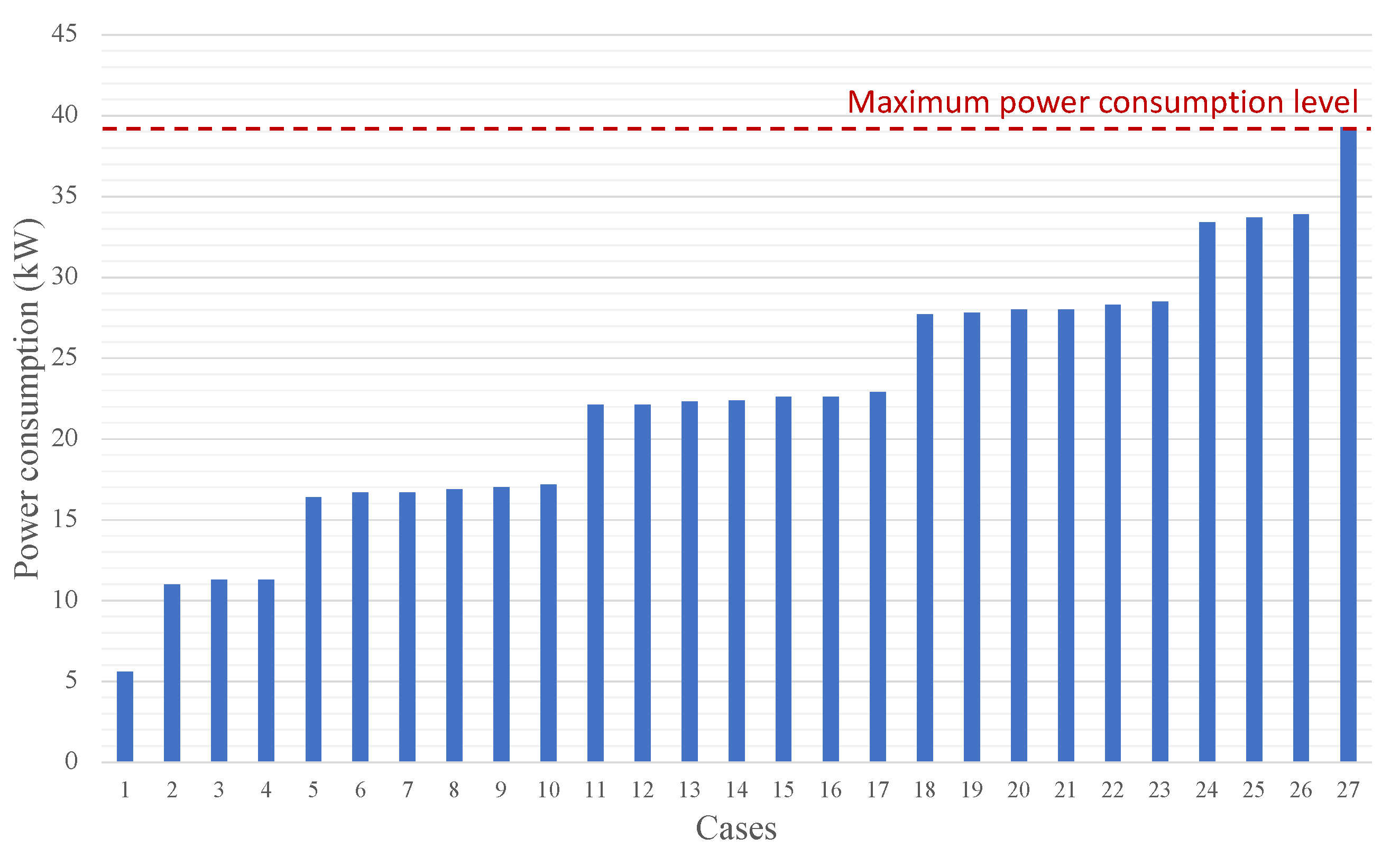
2.2.3. Limitation of the System Design
2.3. The Operation of the Demand Response System
2.3.1. Demand Response Event
2.3.2. Determination of Customer Baseline
3. DR Implementation Details
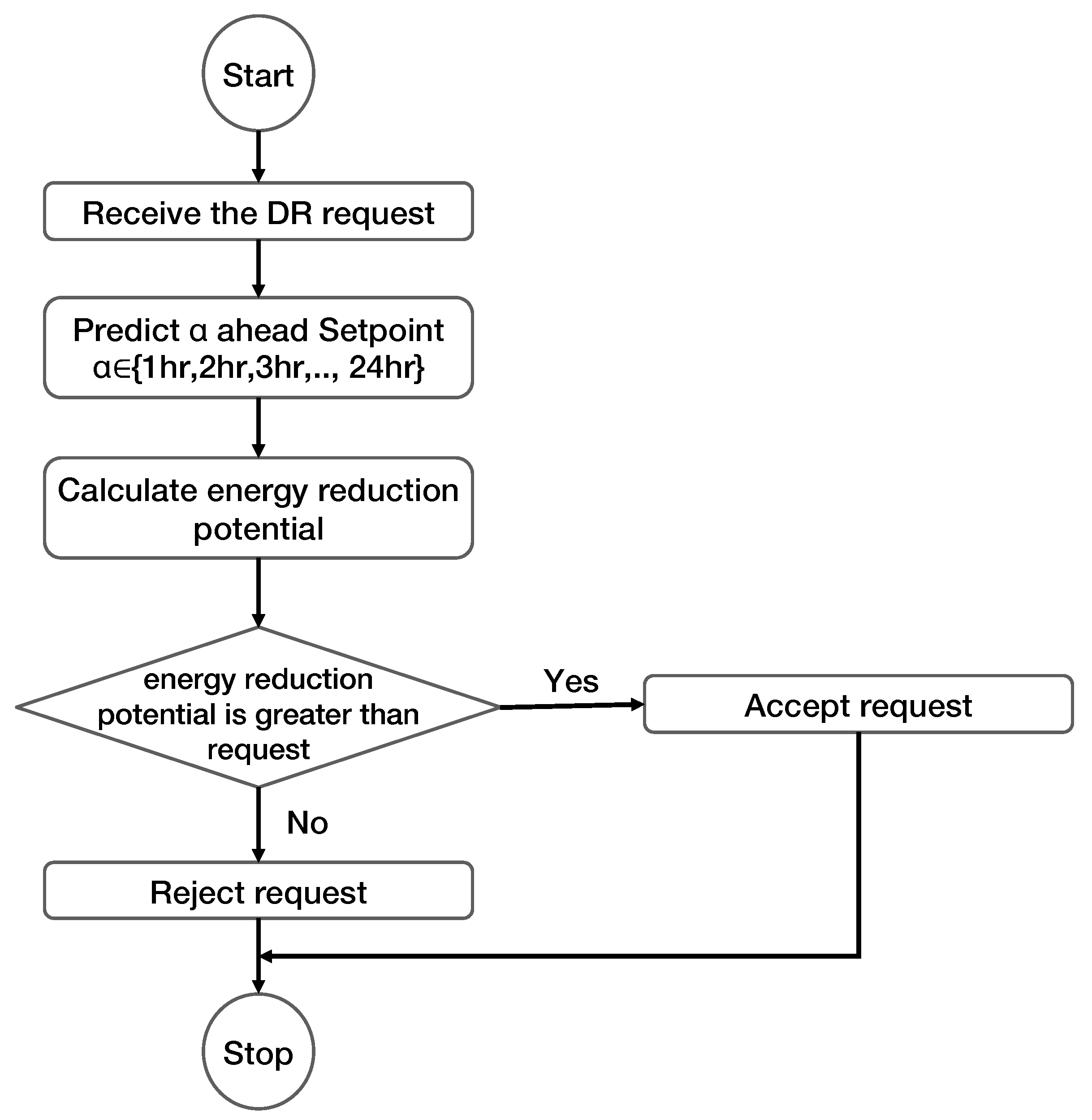
3.1. DR Request Accept/Decline Determination
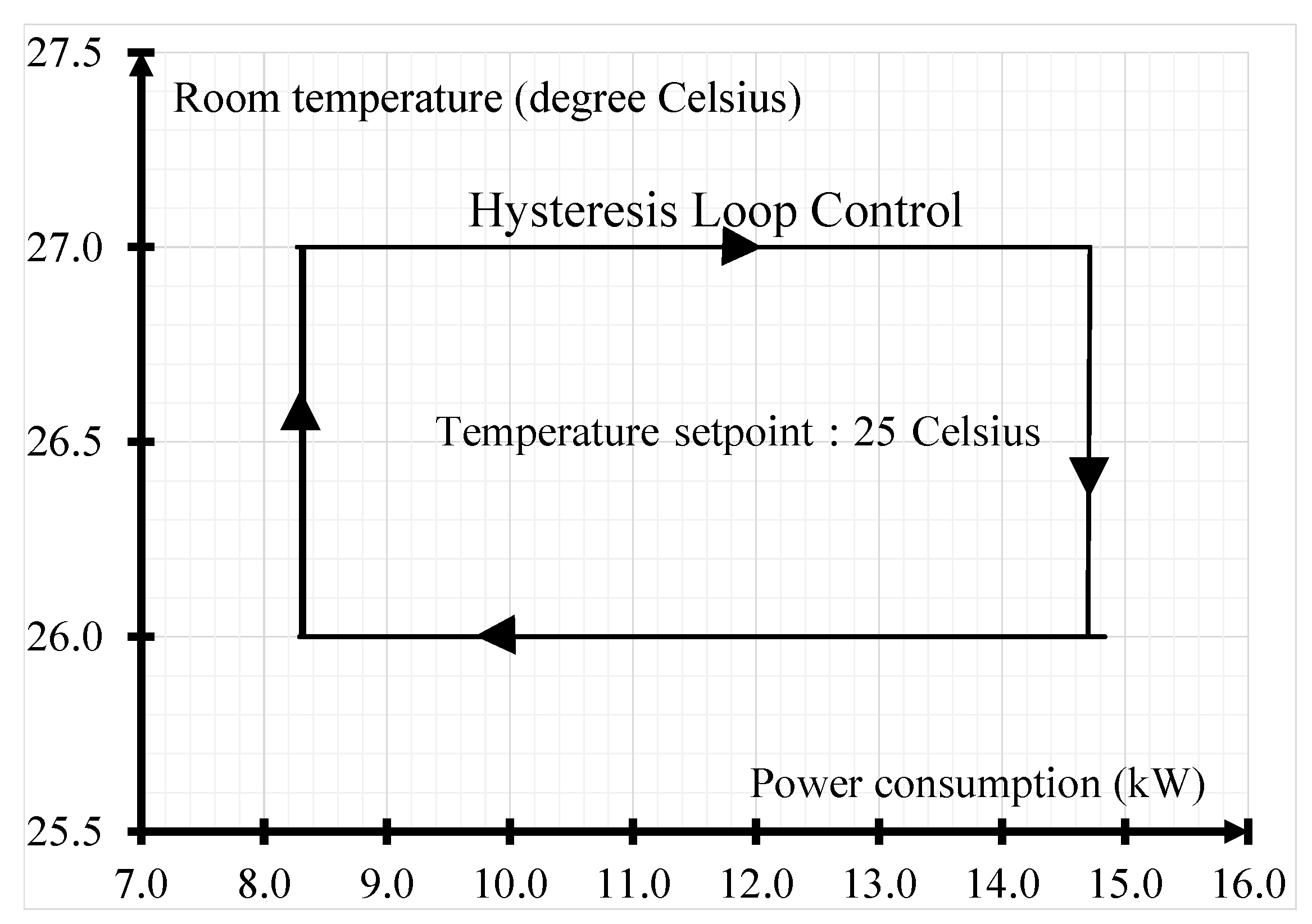
3.2. DR Control Strategy
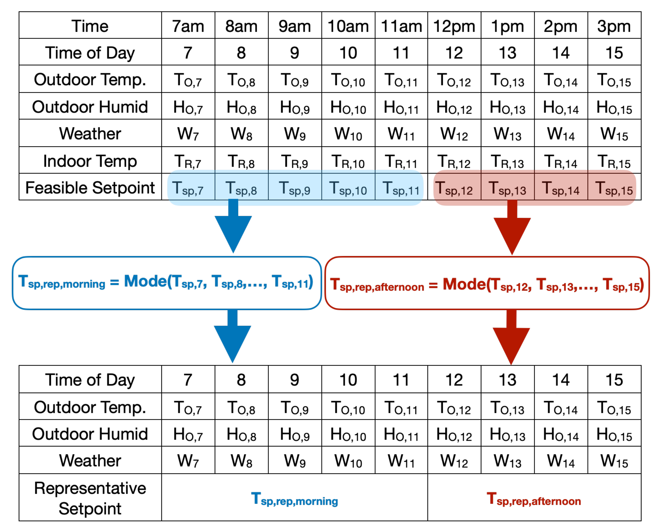
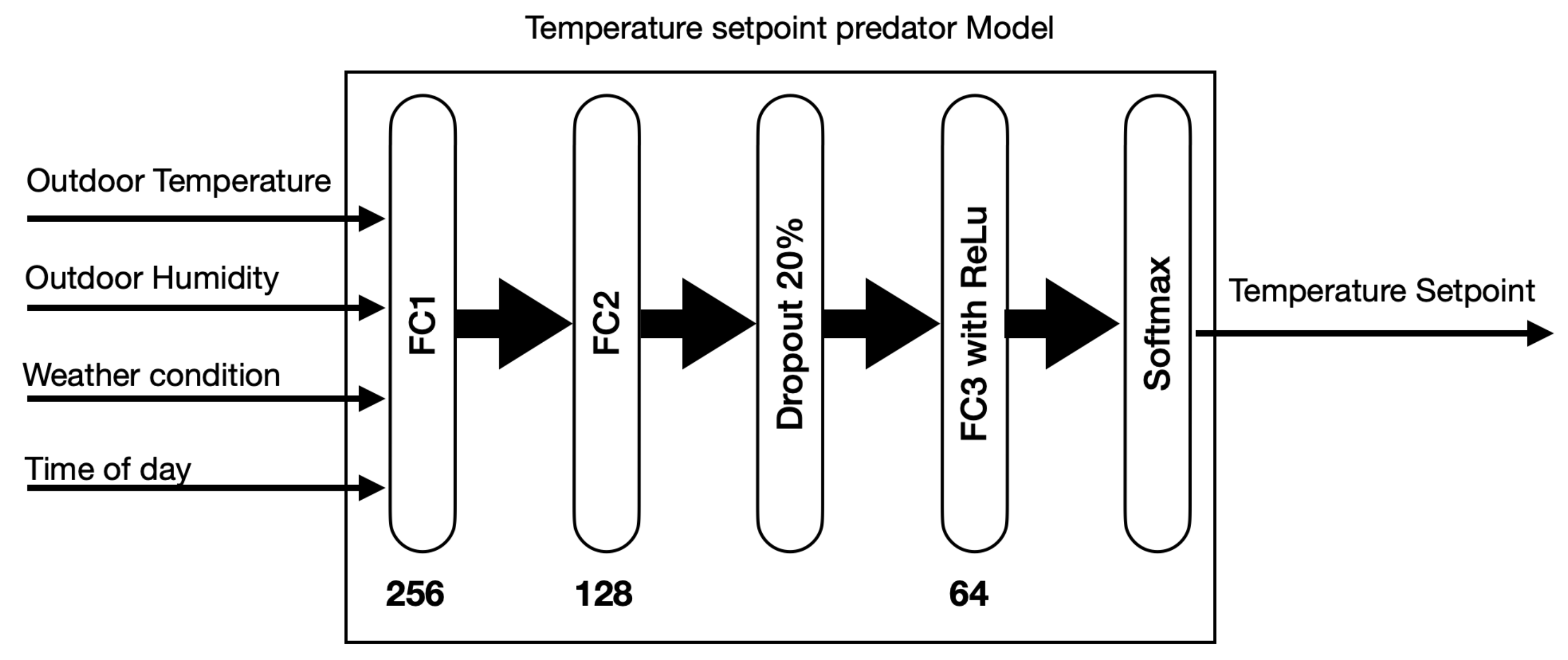
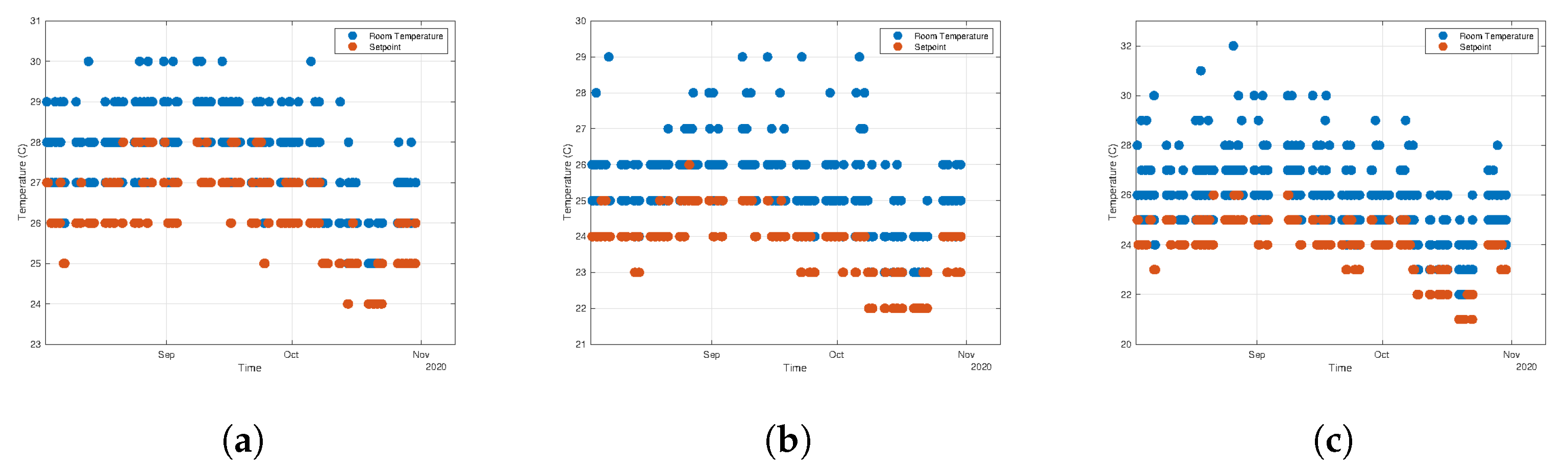
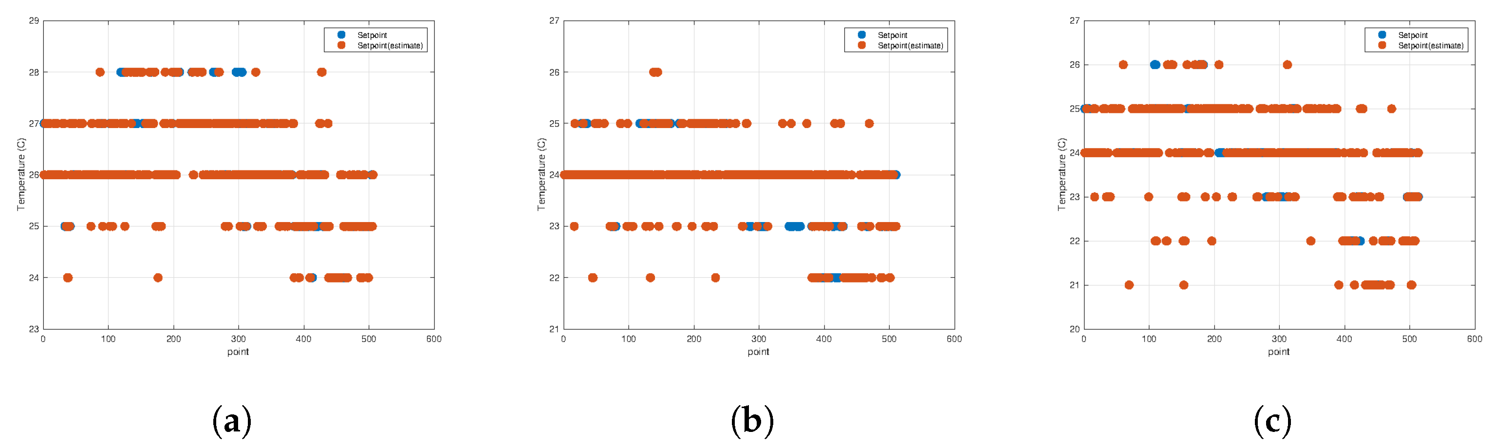
3.3. Determination of AC Temperature Setpoint
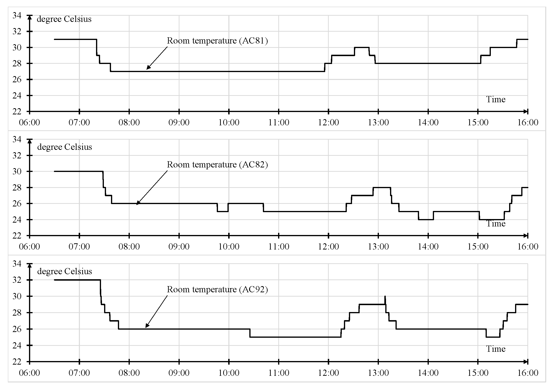
4. Experimental Results and Discussion
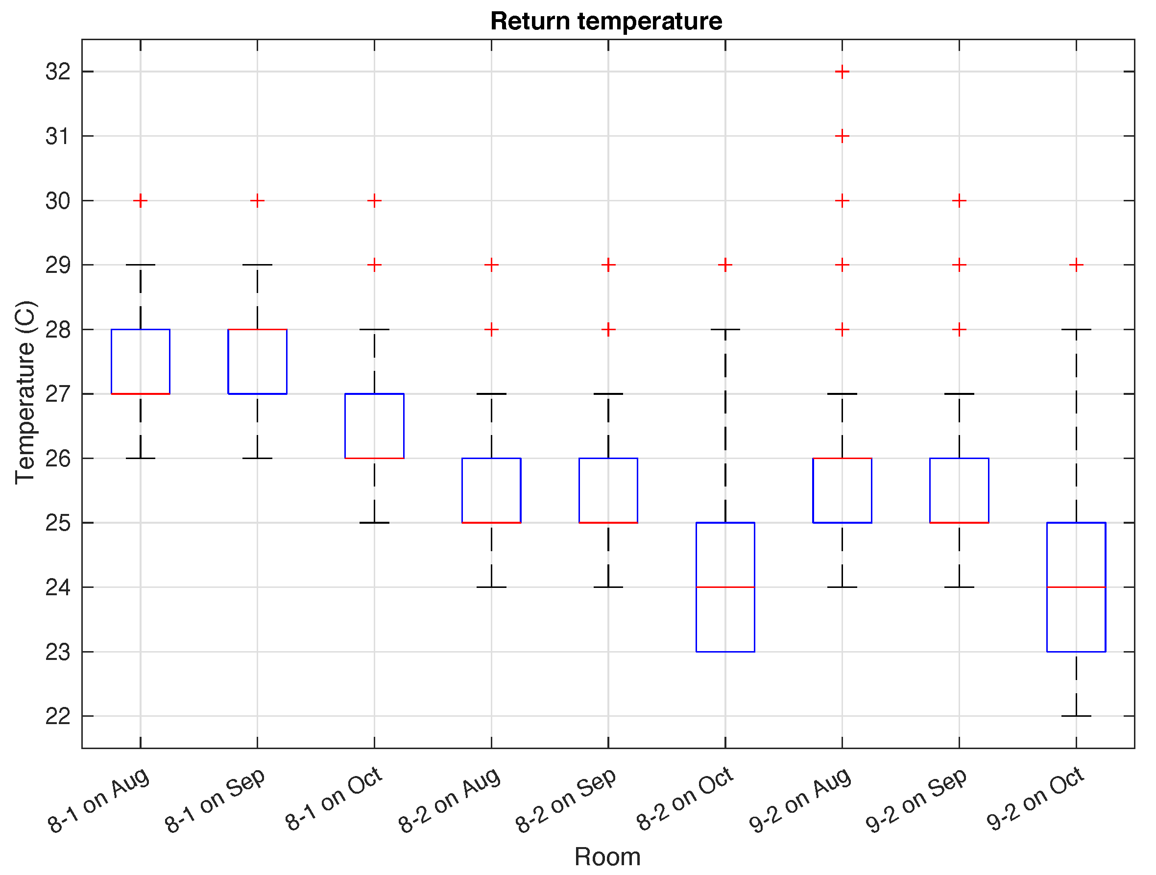
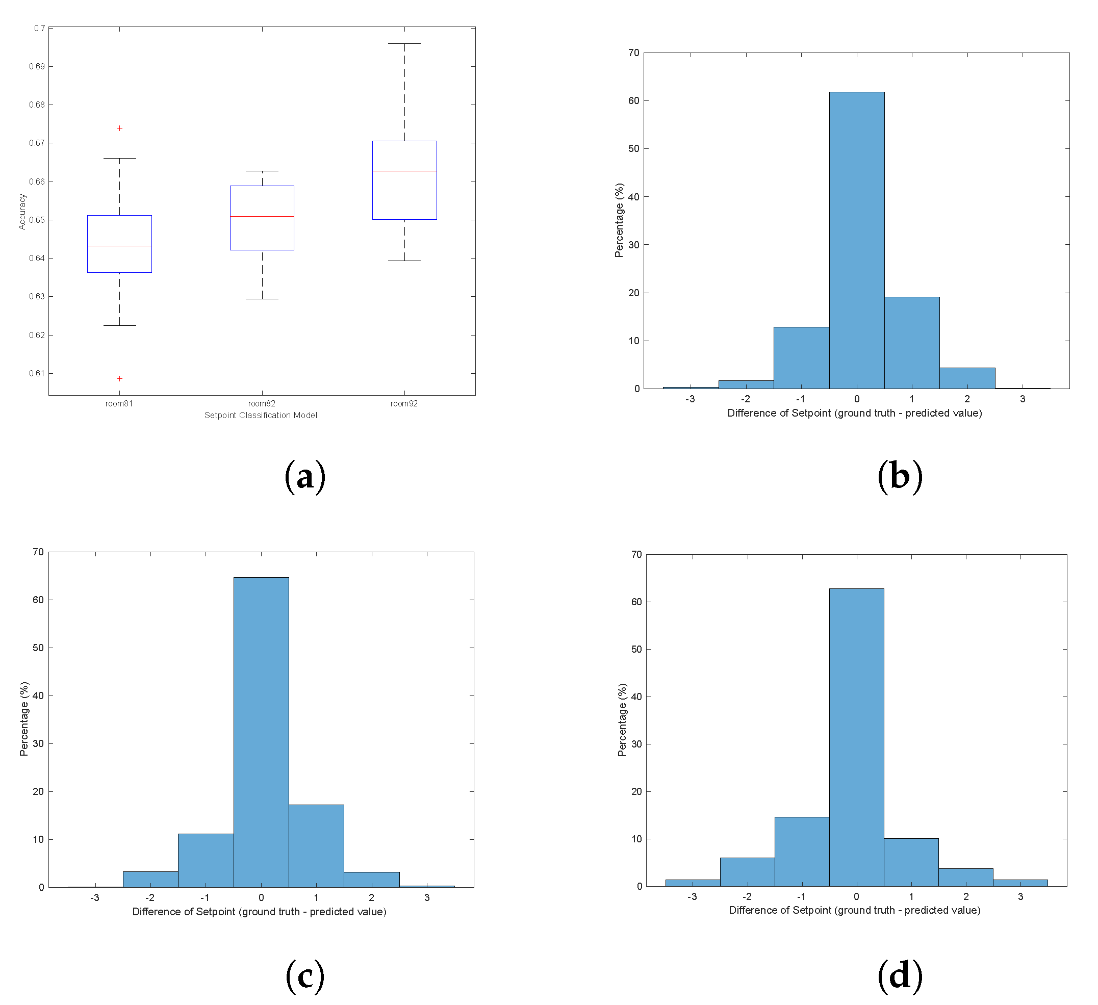
4.1. Experiment on the Temperature Setpoint Estimation
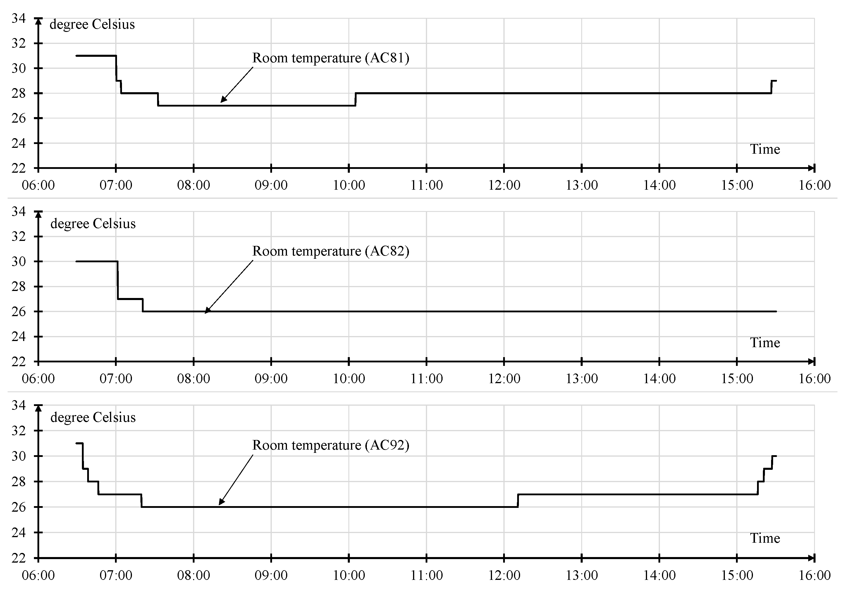
4.2. Experiment on the DR Control
5. Discussion
6. Conclusions
Author Contributions
Funding
Institutional Review Board Statement
Informed Consent Statement
Data Availability Statement
Conflicts of Interest
References
- Motegi, N.; Piette, M.; Watson, D.; Kiliccote, S.; Xu, P. Introduction to Commercial Building Control Strategies and Techniques for Demand Response; LBNL Report Number 59975; Lawrence Berkeley National Laboratory: Berkeley, CA, USA, 2007; pp. 47–54. [CrossRef] [Green Version]
- Albadi, M.; El-Saadany, E. A summary of demand response in electricity markets. Electr. Power Syst. Res. 2008, 78, 1989–1996. [Google Scholar] [CrossRef]
- Wang, S. Making buildings smarter, grid-friendly, and responsive to smart grids. Sci. Technol. Built Environ. 2016, 22, 629–632. [Google Scholar] [CrossRef] [Green Version]
- Shan, K.; Wang, S.; Yan, C.; Xiao, F. Building demand response and control methods for smart grids: A review. Sci. Technol. Built Environ. 2016, 22, 692–704. [Google Scholar] [CrossRef]
- Charoen, P.; Sioutis, M.; Javaid, S.; Charoenlarpnopparut, C.; Lim, Y.; Tan, Y. User-Centric Consumption Scheduling and Fair Billing Mechanism in Demand-Side Management. Energies 2019, 12, 156. [Google Scholar] [CrossRef] [Green Version]
- Ahmad, A.; Hassan, M.; Abdullah, M.; Rahman, H.; Hussin, F.; Abdullah, H.; Saidur, R. A review on applications of ANN and SVM for building electrical energy consumption forecasting. Renew. Sustain. Energy Rev. 2014, 33, 102–109. [Google Scholar] [CrossRef]
- Sherman, R.; Naganathan, H.; Parrish, K. Energy Savings Results from Small Commercial Building Retrofits in the US. Energies 2021, 14, 6207. [Google Scholar] [CrossRef]
- EGAT. Annual Report 2020 Electricity Generating Authority of Thailand; Electricity Generating Authority of Thailand: Bangkok, Thailand, 2020; pp. 22–23. [Google Scholar]
- Sehar, F.; Pipattanasomporn, M.; Rahman, S. An energy management model to study energy and peak power savings from PV and storage in demand responsive buildings. Appl. Energy 2016, 173, 406–417. [Google Scholar] [CrossRef] [Green Version]
- Aduda, K.; Labeodan, T.; Zeiler, W.; Boxem, G.; Zhao, Y. Demand side flexibility: Potentials and building performance implications. Sustain. Cities Soc. 2016, 22, 146–163. [Google Scholar] [CrossRef]
- Aghniaey, S.; Lawrence, T.M. The impact of increased cooling setpoint temperature during demand response events on occupant thermal comfort in commercial buildings: A review. Energy Build. 2018, 173, 19–27. [Google Scholar] [CrossRef]
- Watson, D.; Kiliccote, S.; Motegi, N.; Piette, M.A. Strategies for Demand Response in Commercial Buildings. In 2006 ACEEE Summer Study on Energy Efficiency in Buildings; European Council for an Energy Efficient Economy: Stockholm, Sweden, 2006; pp. 287–299. [Google Scholar]
- Rabl, A.; Norford, L.K. Peak load reduction by preconditioning buildings at night. Int. J. Energy Res. 1991, 15, 781–798. [Google Scholar] [CrossRef]
- Turner, W.; Walker, I.; Roux, J. Peak load reductions: Electric load shifting with mechanical pre-cooling of residential buildings with low thermal mass. Energy 2015, 82, 1057–1067. [Google Scholar] [CrossRef]
- Zhang, J.; Li, X.; Zhao, T.; Yu, H.; Chen, T.; Liu, C.; Yang, X. A Review of Static Pressure Reset Control in Variable Air Volume Air Condition System. Procedia Eng. 2015, 121, 1844–1850. [Google Scholar] [CrossRef] [Green Version]
- Walaszczyk, J.; Cichoń, A. Impact of the duct static pressure reset control strategy on the energy consumption by the HVAC system. E3S Web Conf. 2017, 17, 00095. [Google Scholar] [CrossRef] [Green Version]
- Xue, X.; Wang, S.; Yan, C.; Cui, B. A fast chiller power demand response control strategy for buildings connected to smart grid. Appl. Energy 2015, 137, 77–87. [Google Scholar] [CrossRef]
- Maneebang, K.; Methapatara, K.; Kudtongngam, J. A Demand Side Management Solution: Fully Automated Demand Response using OpenADR2.0b Coordinating with BEMS Pilot Project. In Proceedings of the 2020 International Conference on Smart Grids and Energy Systems (SGES), Perth, Australia, 23–26 November 2020; pp. 30–35. [Google Scholar] [CrossRef]
- Alamin, Y.I.; Castilla, M.D.M.; Álvarez, J.D.; Ruano, A. An Economic Model-Based Predictive Control to Manage the Users’ Thermal Comfort in a Building. Energies 2017, 10, 321. [Google Scholar] [CrossRef]
- Kim, J.; Song, D.; Kim, S.; Park, S.; Choi, Y.; Lim, H. Energy-Saving Potential of Extending Temperature Set-Points in a VRF Air-Conditioned Building. Energies 2020, 13, 2160. [Google Scholar] [CrossRef]
- Turley, C.; Jacoby, M.; Pavlak, G.; Henze, G. Development and Evaluation of Occupancy-Aware HVAC Control for Residential Building Energy Efficiency and Occupant Comfort. Energies 2020, 13, 5396. [Google Scholar] [CrossRef]
- Macieira, P.; Gomes, L.; Vale, Z. Energy Management Model for HVAC Control Supported by Reinforcement Learning. Energies 2021, 14, 8210. [Google Scholar] [CrossRef]
- Yang, K.; Su, C. An approach to building energy savings using the PMV index. Build. Environ. 1997, 32, 25–30. [Google Scholar] [CrossRef]
- van Hoof, J. Forty years of Fanger’s model of thermal comfort: Comfort for all? Indoor Air 2008, 18, 182–201. [Google Scholar] [CrossRef]
- Toftum, J.; Andersen, R.; Jensen, K. Occupant performance and building energy consumption with different philosophies of determining acceptable thermal conditions. Build. Environ. 2009, 44, 2009–2016. [Google Scholar] [CrossRef]
- Brager, G.S.; de Dear, R.J. Thermal adaptation in the built environment: A literature review. Energy Build. 1998, 27, 83–96. [Google Scholar] [CrossRef] [Green Version]
- Hafeez, G.; Javaid, N.; Iqbal, S.; Khan, F.A. Optimal Residential Load Scheduling Under Utility and Rooftop Photovoltaic Units. Energies 2018, 11, 611. [Google Scholar] [CrossRef] [Green Version]
- Wasim Khan, H.; Usman, M.; Hafeez, G.; Albogamy, F.R.; Khan, I.; Shafiq, Z.; Usman Ali Khan, M.; Alkhammash, H.I. Intelligent Optimization Framework for Efficient Demand-Side Management in Renewable Energy Integrated Smart Grid. IEEE Access 2021, 9, 124235–124252. [Google Scholar] [CrossRef]
- Hafeez, G.; Alimgeer, K.S.; Wadud, Z.; Khan, I.; Usman, M.; Qazi, A.B.; Khan, F.A. An Innovative Optimization Strategy for Efficient Energy Management With Day-Ahead Demand Response Signal and Energy Consumption Forecasting in Smart Grid Using Artificial Neural Network. IEEE Access 2020, 8, 84415–84433. [Google Scholar] [CrossRef]
- Hafeez, G.; Alimgeer, K.S.; Khan, I. Electric load forecasting based on deep learning and optimized by heuristic algorithm in smart grid. Appl. Energy 2020, 269, 114915. [Google Scholar] [CrossRef]
- Hafeez, G.; Islam, N.; Ali, A.; Ahmad, S.; Usman, M.; Saleem Alimgeer, K. A Modular Framework for Optimal Load Scheduling under Price-Based Demand Response Scheme in Smart Grid. Processes 2019, 7, 499. [Google Scholar] [CrossRef] [Green Version]
- Coughlin, K.; Piette, M.A.; Goldman, C.; Kiliccote, S. Statistical analysis of baseline load models for non-residential buildings. Energy Build. 2009, 41, 374–381. [Google Scholar] [CrossRef] [Green Version]
- Wijaya, T.K.; Vasirani, M.; Aberer, K. When Bias Matters: An Economic Assessment of Demand Response Baselines for Residential Customers. IEEE Trans. Smart Grid 2014, 5, 1755–1763. [Google Scholar] [CrossRef]
- Mohajeryami, S.; Doostan, M.; Schwarz, P. The impact of Customer Baseline Load (CBL) calculation methods on Peak Time Rebate program offered to residential customers. Electr. Power Syst. Res. 2016, 137, 59–65. [Google Scholar] [CrossRef]
- Mohajeryami, S.; Cecchi, V. An investigation of the Randomized Controlled Trial (RCT) method as a Customer Baseline Load (CBL) calculation for residential customers. In Proceedings of the 2017 IEEE Power Energy Society General Meeting, Chicago, IL, USA, 16–20 July 2017; pp. 1–5. [Google Scholar] [CrossRef] [Green Version]
- Mohajeryami, S.; Doostan, M.; Asadinejad, A.; Schwarz, P. Error Analysis of Customer Baseline Load (CBL) Calculation Methods for Residential Customers. IEEE Trans. Ind. Appl. 2017, 53, 5–14. [Google Scholar] [CrossRef]
- Ministry of Energy, Thailand. National Smart Grid Master Plan (2015–2036); 2015. Available online: http://www.eppo.go.th/index.php/en/about-us/company-profile (accessed on 19 December 2021).
- Ministry of Energy, Thailand. National Smart Grid Action Plan (2017–2021); Ministry of Energy: Bangkok, Thailand, 2016.
- Mustafaraj, G.; Lowry, G.; Chen, J. Prediction of room temperature and relative humidity by autoregressive linear and nonlinear neural network models for an open office. Energy Build. 2011, 43, 1452–1460. [Google Scholar] [CrossRef]
- Ashtiani, A.; Mirzaei, P.A.; Haghighat, F. Indoor thermal condition in urban heat island: Comparison of the artificial neural network and regression methods prediction. Energy Build. 2014, 76, 597–604. [Google Scholar] [CrossRef]
- Kong, W.; Dong, Z.Y.; Jia, Y.; Hill, D.J.; Xu, Y.; Zhang, Y. Short-Term Residential Load Forecasting Based on LSTM Recurrent Neural Network. IEEE Trans. Smart Grid 2019, 10, 841–851. [Google Scholar] [CrossRef]
- Wang, Y.; Gan, D.; Sun, M.; Zhang, N.; Lu, Z.; Kang, C. Probabilistic individual load forecasting using pinball loss guided LSTM. Appl. Energy 2019, 235, 10–20. [Google Scholar] [CrossRef] [Green Version]
- Srivastava, N.; Hinton, G.; Krizhevsky, A.; Sutskever, I.; Salakhutdinov, R. Dropout: A Simple Way to Prevent Neural Networks from Overfitting. J. Mach. Learn. Res. 2014, 15, 1929–1958. [Google Scholar]
- Nair, V.; Hinton, G.E. Rectified Linear Units Improve Restricted Boltzmann Machines. In Proceedings of the 27th International Conference on International Conference on Machine Learning (ICML’10), Haifa, Israel, 21–24 June 2010; Omnipress: Madison, WI, USA, 2010; pp. 807–814. [Google Scholar]
- Kingma, D.P.; Ba, J. Adam: A Method for Stochastic Optimization. arXiv 2017, arXiv:1412.6980. [Google Scholar]


| Equipment | Detail/Sizing | Quantity | Remark |
|---|---|---|---|
| AC81 | Trane® 30 kW (PWC-81) | 1 | existing system |
| AC82 | Trane® 30 kW (PWC-82) | 1 | existing system |
| AC92 | Trane® 30 kW (PWC-92) | 1 | existing system |
| Power meter | SATEC EM133 | 3 | exiting system |
| DR gateway | Dell precision workstation PC | 1 | new investment |
| IoT device | Siemens SIMATIC IoT | 5 | new investment |
| Ethernet switch | Dell 8-gigabits port | 1 | new investment |
| Communication device | TP-Link deco mesh Wi-Fi | 3 | new investment |
| Air Conditioner Code | Air Blower (kW) | One Compressor (kW) | Two Compressors (kW) |
|---|---|---|---|
| PWC-81 | 1.9 | 7.3 | 12.7 |
| PWC-82 | 1.9 | 7.3 | 13.5 |
| PWC-92 | 1.8 | 7.5 | 13.1 |
| Condition | - | Return Temperature −1 | Return Temperature |
| Criteria | The Number of Samples | ||
|---|---|---|---|
| Room 81 | Room 82 | Room 92 | |
| Total | 8831 | 8831 | 8831 |
| ACs operating | 1687 | 1700 | 1712 |
| Training dataset | 1181 | 1190 | 1199 |
| Testing dataset | 506 | 510 | 513 |
| Layer No. | Layer Name | Configuration |
|---|---|---|
| 1 | Feature Input | 4 features with z-score normalization |
| 2 | Fully Connected | 256 fully connected layer |
| 3 | Fully Connected | 128 fully connected layer |
| 4 | Dropout | 20% dropout |
| 5 | Fully Connected | 64 fully connected layer |
| 6 | ReLU | - |
| 7 | Fully Connected | 6 fully connected layer |
| 8 | Softmax | - |
| 9 | Classification Output | Cross Entropy loss function |
| Parameter | Value |
|---|---|
| Decay rate of gradient moving average () | 0.9 |
| Decay rate of squared gradient moving average () | 0.999 |
| Epsilon | 1.0 × 10 |
| Initial learning rate | 0.005 |
| Gradient Threshold Method | L2-norm |
| Gradient Threshold | 1 |
| Factor for L2 regularizer (weight decay) | 1.0 × 10 |
| Max Epochs | 500 |
Publisher’s Note: MDPI stays neutral with regard to jurisdictional claims in published maps and institutional affiliations. |
© 2022 by the authors. Licensee MDPI, Basel, Switzerland. This article is an open access article distributed under the terms and conditions of the Creative Commons Attribution (CC BY) license (https://creativecommons.org/licenses/by/4.0/).
Share and Cite
Charoen, P.; Kitbutrawat, N.; Kudtongngam, J. A Demand Response Implementation with Building Energy Management System. Energies 2022, 15, 1220. https://doi.org/10.3390/en15031220
Charoen P, Kitbutrawat N, Kudtongngam J. A Demand Response Implementation with Building Energy Management System. Energies. 2022; 15(3):1220. https://doi.org/10.3390/en15031220
Chicago/Turabian StyleCharoen, Prasertsak, Nathavuth Kitbutrawat, and Jasada Kudtongngam. 2022. "A Demand Response Implementation with Building Energy Management System" Energies 15, no. 3: 1220. https://doi.org/10.3390/en15031220