Ergonomic and Economic Office Light Level Control

Abstract

Light regulation systems in industrial or office buildings play an important role in minimizing the use of fossil energy resources, while providing both economic and ergonomic optimal functionality. Although industrial buildings resolve the problem of interaction or disturbance mitigation by providing constant light levels exclusively from artificial sources, office landscapes may benefit from up to a 20% decrease in costs if mixed light sources are optimized properly. In this paper, we propose a theoretical framework based on model predictive control (MPC) to resolve a multi-system with strong dynamic interactions and multi-objective cost optimization. Centralized and distributed predictive control strategies are compared on various office landscaping structures and functionality conditions. Economic and ergonomic indexes are evaluated in a scaled laboratory setting.

1. Introduction

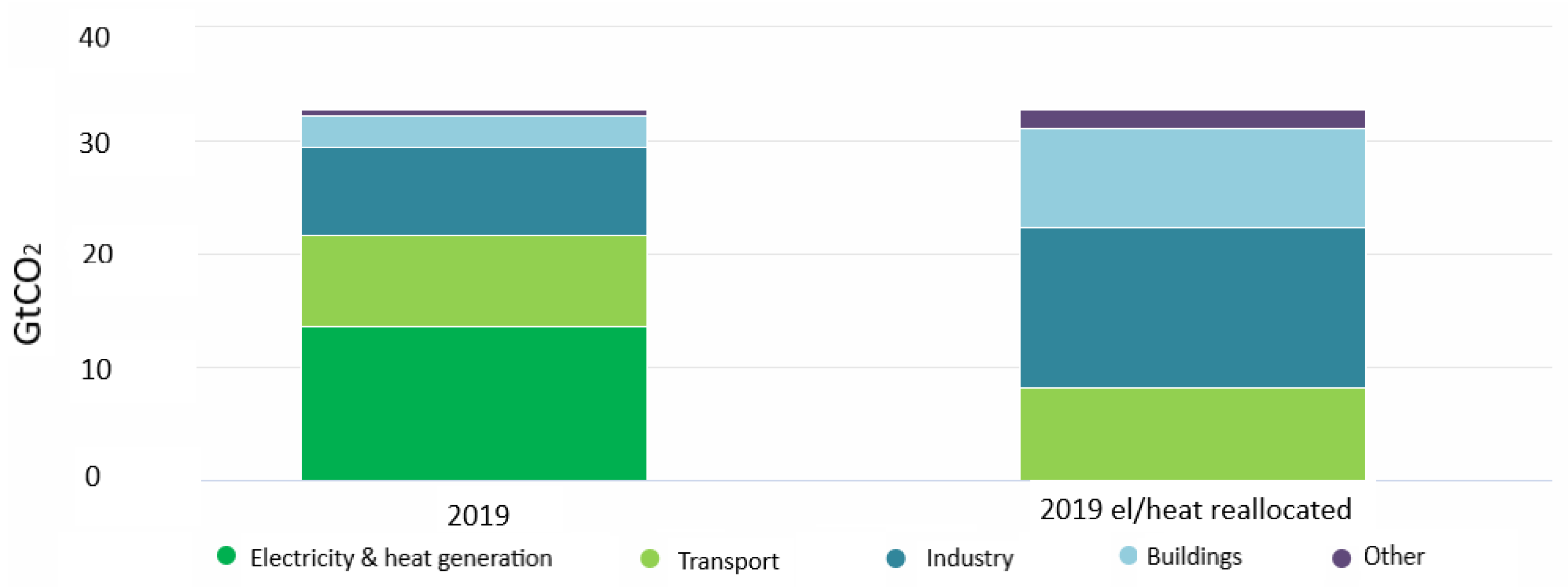
In recent years, the climate has become one of the most discussed topics in world politics. It is clear that CO${}_2$ emissions should be reduced drastically. Approximately 40% of total CO${}_2$ emissions worldwide are caused by the production of electricity and heat, as summarized in Figure 1 (left stacked bar chart) [1].

On the other hand, Belgium is one of the leading European countries in terms of green energy production and minimizing fossil energy use (see the right stacked bar chart in Figure 1). The electricity consumption for lighting in office buildings accounts for about 25% of the total energy consumption within these premises [2,3]. Two main solutions to reduce both the electricity costs and its ecological footprint are:

• Power-saving lights, i.e., lights based on recently emerging light-emitting diode (LED) technology. These LED-lights exhibit an energy decrease of over 85% and last about 20 times as long [4] as standard lights; and
• Smart light regulators, i.e., regulating light levels according to the function of the area and functionality of the area. An advanced light controller acts according to the operator requests or predefined functionality per office area [5].

Industrial relevance, in terms of the need for regulatory solutions, is shown by the top three most accepted and versatile methodologies: proportional-integral-derivative (PID) control, predictive control, and system identification [6]. Although it is a successful technology and it is deeply embedded in the lower loop control objective platforms of any dynamic process control problem, PID control has serious limitations in dealing with strongly interacting systems and multi-objective optimization problems. Through system identification, advanced control technologies such as model-based control, i.e., predictive control, represent a rather ubiquitous solution in multi-system, multi-level, and multi-objective optimization methods for control problems [7].

Previous attempts to regulate light levels in office landscape areas have provided solutions based on PID control and generalized order PID-type controllers, with successful performance in terms of reference setpoint tracking [8,9]. In addition, a large number of applications have made use of lighting control techniques, such as conventional methods, implementations of intelligent techniques, and agent-based controllers [10], taking into consideration the features of the environment. In order to improve building designs and networked sensor-actuator systems by increasing the energy efficiency and the comfort of the building occupants, techniques based on hierarchical structures [11] and systems with decentralized integral controllers [12] have been developed in recent years. Modern developments have proposed different decision-making strategies for optimizing the performance of lighting systems in wide urban areas, such as a large-scale street [13] and a university campus [14], taking into consideration both energy savings and user satisfaction. However, to adequately analyze its economic and ergonomic impact, predictive control seems to be a natural solution. Office buildings often have functionality with repetitive dynamics, which can be implemented by learning algorithms, or iterative optimization algorithms. On the other hand, the use of renewable energy resources is often dependent on stochastic disturbances (e.g., sunlight) with piecewise periodic dynamics (e.g., day/night, season, office hours). Although not directly acknowledged in conscious task operation, the flickering of light levels from inadequate dimmer control or external sources of light level variations (windmill periodic shadow, weather) affects operator productivity. Often, the commonly encountered solution in industry is to avoid these issues by using facilities with only artificial light sources. However, in-office buildings, windows can be a great source of external light if used properly.

In this paper, we propose a theoretical framework to resolve a multi-system with strong dynamic interactions and multi-objective cost. Distributed predictive control strategies are compared with various office landscaping structures and functionality conditions. Economic and ergonomic indexes were evaluated in both a simulation and an experimental setup scaled in a laboratory setting. The original contribution of the paper is a fast, distributed predictive control algorithm, used to compare the changes in the light level for different landscape office structures, with changing context parameters (e.g., introducing external sunlight).

The paper is structured as follows. Section 2 presents the office landscape setup control problem and describes the control and optimization methodologies. Next, the results are presented in Section 3 and Section 4 discusses the main outcomes of this work.

2. Materials and Methods

2.1. Study Case

The laboratory test setup mimics the lighting structure in a typical office environment. This laboratory-scale system was inspired by that proposed in [15] and simplified to a box with eight light bulbs and eight sensors, as depicted in Figure 2. The environment is composed of eight zones, each consisting of a lamp and a sensor distributed unevenly in each delimited room. This design permits us to consider “wall” constructions with varying heights for delineating the influence between zones of illumination and the superposition of light zones. Open environments or divided structures are possible to mimic, but an increased division of the zones will limit the influence between them. In addition, the performance of the box has been improved by adding two ways of simulating daylight, with the possibility of showing its effects on the test setup system, as a disturbance. The first one is to emulate the daylight electrically using the two additional lamps represented as “D” and the last one is using the windows on the sides of the box to allow daylight inside the rooms where we want to analyze its effects on the system. The positions of the lamps, windows, and sensors are presented in Figure 3.

A system, depicted in Figure 4, was built to measure the light intensity in the room at the location of the window, with a sampling rate of 500 Hz. This system consists of four components: (i) a Raspberry Pi zero W; (ii) a power bank (20,800 mAh); (iii) a 16 GB micro SD for storing data and (iv) a light sensor (BH1750FVI) measuring light intensity between 1 and 65,535 lx.

2.2. Modeling

The system is a strongly coupled dynamic multivariable process, in which the light intensity will cross-couple across zones of the setup area. To calculate the interaction coefficients, a staircase experiment was applied and the measured outputs of every light for the case with office walls (half-height) are depicted in Figure 5. The identification of these coefficients is performed as follows: a staircase signal is applied to the input of one zone, while the other zones are kept at a zero input. This is carried out once for each system’s input. The output values of each zone are plotted, resulting in a total of eight figures. The coefficients belonging to system i’s input and system j’s output are calculated as follows. First, the value of system j’s output at the third step of the staircase is determined from the experiment with system i as the input. The third step was chosen as it lies in the middle of the input range. Next, the obtained values are normalized with the output value of the third step of system 1 with system 1 as the input. Note that if the height of the walls is changed, the interaction gains are changed. An additional pseudorandom binary sequence (PRBS) test signal is used to perform identification.

This system can be represented by means of a Hammerstein system [16]:

$$y_j\left(s\right)=\sum _{i=1}^8\left(L\left\{f\left(u_i\left(t\right)\right)\right\}\left(s\right)P\left(s\right)K_{ij}\right)$$

(1)

where $y_j$ is the output of the sensor in zone j, $u_i$ is the input of the lamp in zone i and f is a linear correlation function:

$$f\left(x\right)=0.5334x-0.2388$$

(2)

The interaction gain is represented by the coupling matrix K, which is obtained from the staircase experiment and which, for the case of half-height walls, has the values:

$$K_{ij}=\left[\begin{array}{cccccccc}1.19& 0.34& 0.11& 0.06& 0.63& 0.25& 0.11& 0.05\\ 0.86& 1.11& 0.43& 0.15& 0.49& 0.60& 0.26& 0.10\\ 0.18& 0.45& 1.15& 0.53& 0.12& 0.24& 0.67& 0.29\\ 0.08& 0.12& 0.52& 1.34& 0.06& 0.08& 0.29& 0.78\\ 0.31& 0.16& 0.09& 0.07& 1.18& 0.51& 0.14& 0.07\\ 0.23& 0.24& 0.18& 0.11& 0.70& 1.11& 0.77& 0.13\\ 0.12& 0.19& 0.32& 0.24& 0.13& 0.37& 1.08& 0.40\\ 0.06& 0.08& 0.22& 0.43& 0.06& 0.12& 0.51& 1.19\end{array}\right]$$

(3)

The process transfer function model is represented by $P\left(s\right)$ and is considered to be the same for the dynamics of all the lamps:

$$P\left(s\right)=\frac{33.09}{s+32.63}$$

(4)

2.3. Configurations

Several configurations have been investigated, representing various arrangements of office landscapes, which could also have differing functionality (e.g., office desk, coffee table, printer area), thereby requiring different light levels. These configurations are represented in Figure 6 and are studied in this work.

2.4. Predictive Control Basics

Consider the generic 2×2 process model:

$$\left\{\begin{array}{c}{y}_1\left(t\right)=x_1\left(t\right)+n_1\left(t\right)\hfill \\ y_2\left(t\right)=x_2\left(t\right)+n_2\left(t\right)\hfill \end{array}\right.$$

(5)

where $x_i\left(t\right)$ is the model output, $y_i\left(t\right)$ is the process output and $n_i\left(t\right)$ represents the process/model disturbance. The process models are defined as a function of past model predictions and past inputs:

$$\left\{\begin{array}{c}{y}_1\left(t\right)=f_1[x_1(t-1),x_1(t-2),\dots ,u_1(t-1),u_1(t-2),\dots ,u_2(t-1),u_2(t-2),\dots ]\hfill \\ y_2\left(t\right)=f_2[x_2(t-1),x_2(t-2),\dots ,u_1(t-1),u_1(t-2),\dots ,u_2(t-1),u_2(t-2),\dots ]\hfill \end{array}\right.$$

(6)

The disturbance model is represented as colored noise, where $e_i\left(t\right)$ is white noise and $C_i\left(q^{-1}\right)$ and $D_i\left(q^{-1}\right)$ are monic polynomials in the shift operator q:

$$n_1\left(t\right)=\frac{C_1\left(q^{-1}\right)}{D_1\left(q^{-1}\right)}{e}_1\left(t\right)\mathrm{and}{n}_2\left(t\right)=\frac{C_2\left(q^{-1}\right)}{D_2\left(q^{-1}\right)}{e}_2\left(t\right)$$

(7)

This filter can be designed in various ways as a function of the type of expected disturbance profile [17]. The elements in $u_i(t+k|t)$ are the optimal control actions, represented as the sum of basic control actions $u_{ibase}(t+k|t)$ and optimizing control actions $\delta u_i(t+k|t)$:

$$\left\{\begin{array}{c}{u}_1(t+k|t)=u_{1base}(t+k|t)+\delta u_1(t+k|t)\hfill \\ u_2(t+k|t)=u_{2base}(t+k|t)+\delta u_2(t+k|t)\hfill \end{array}\right.$$

(8)

These control actions will lead to an optimal response $y_i(t+k|t)$, which is the sum of the base response $y_{ibase}(t+k|t)$ and the optimizing response $y_{iopt}(t+k|t)$:

$$\left\{\begin{array}{c}{y}_1(t+k|t)=y_{1base}(t+k|t)+y_{1opt}(t+k|t)\hfill \\ y_2(t+k|t)=y_{2base}(t+k|t)+y_{1opt}(t+k|t)\hfill \end{array}\right.$$

(9)

with $y_{1opt}(t+1|t)$ calculated as follows:

$$\begin{array}{cc}\hfill \left[\begin{array}{c}{y}_{1opt}(t+1|t)\\ y_{1opt}(t+2|t)\\ \dots \\ \dots \\ y_{1opt}(t+N_2|t)\end{array}\right]& =\left[\begin{array}{ccccc}{h}_1^{11}& 0& 0& \dots & 0\\ h_2^{11}& h_1^{11}& 0& \dots & 0\\ \dots & \dots & \dots & \dots & \dots \\ \dots & \dots & \dots & \dots & \dots \\ h_{N_2}^{11}& h_{N_2-1}^{11}& h_{N_2-2}^{11}& \dots & g_{N_2-N_u+1}^{11}\end{array}\right]·\left[\begin{array}{c}\delta u_1\left(t\right|t)\\ \delta u_1(t+1|t)\\ \dots \\ \dots \\ \delta u_1(t+N_u-1|t)\end{array}\right]\hfill \\ \hfill & +\left[\begin{array}{ccccc}{h}_1^{12}& 0& 0& \dots & 0\\ h_2^{12}& h_1^{12}& 0& \dots & 0\\ \dots & \dots & \dots & \dots & \dots \\ \dots & \dots & \dots & \dots & \dots \\ h_{N_2}^{12}& h_{N_2-1}^{12}& h_{N_2-2}^{11}& \dots & g_{N_2-N_u+1}^{12}\end{array}\right]·\left[\begin{array}{c}\delta u_2\left(t\right|t)\\ \delta u_2(t+1|t)\\ \dots \\ \dots \\ \delta u_2(t+N_u-1|t)\end{array}\right]\hfill \end{array}$$

(10)

where the parameters h are the coefficients of the unit impulse response and the parameters g are the unit step response of the system. A similar expression can be obtained for $y_{2opt}(t+1|t)$. The control horizon $N_c$ determines after which step the control action remains constant. The prediction horizon $N_2$ determines the number of samples of the future control actions that are calculated. In matrix notation, the key equations are:

$$\left\{\begin{array}{c}{Y}_1=Y_{1base}+G_{11}·U_1+G_{12}·U_2\hfill \\ Y_2=Y_{2base}+G_{21}·U_1+G_{22}·U_2\hfill \end{array}\right.$$

(11)

The extended prediction self-adaptive control (EPSAC) algorithm is implemented hereafter, and was previously validated in several simulations and experimental applications [18,19,20].

2.5. Distributed Control Scheme

An effective distributed model predictive control (DiMPC) scheme was proposed in [21], as illustrated in Figure 7. Every dynamic subsystem has its own controller, which calculates the optimal solution for its own subsystem, based on the information received from neighboring sub-systems. To reach the optimal solution, the optimization algorithm is performed iteratively.

The iterative DiMPC structure consists of five steps. These steps can be implemented for one objective, or for prioritized sequential objectives, as in Figure 8.

• Step 1: Subsystem i receives an optimal local control action $\delta U_i$ at the iterative time as $iter$ = 0 according to the EPSAC algorithm, and the local control action $\delta U_i$ can be rewritten as $\delta U_i^{iter}$, where $\delta U_i$ indicates the vector of the optimizing future control actions with a length of $N_{ci}$;
• Step 2: The $\delta U_j^{iter}$ (j $ϵ$$N_i$) is communicated to the subsytem i, and the $\delta U_i^{iter+1}$ is calculated again with the $\delta U_j^{iter}$ from the other subsystems;
• Step 3: If the terminal conditions $\left|\right|$$\delta U_i^{iter+1}-\delta U_i^{iter}$$\left|\right|$≤${\epsilon }_i$∨$iter+1>\overline{iter}$ are reached, the $U_i^{iter+1}$ is adopted, where ${\epsilon }_i$ is the positive value and $\overline{iter}$ indicates the upper bound of the number of iterations. Otherwise, the iter is set as $iter$ = $iter$ + 1, and return to step 2;
• Step 4: Calculate the optimal control effort as $U_t$ = $U_{base}$ + $\delta U^{iter}$, and the control effort is applied to the system;
• Step 5: Set the discrete time sample $t=t+1$ and return to step 1.

The number of iterations is often limited in practice to a trade-off number between the computational time and solution optimality.

2.6. Multi-Objective Optimization

The computation time is a key element when one deploys control algorithms in real-time platforms. A practical set of multi-objective optimization algorithms for industrial multivariable PID control is proposed in [22]. For predictive control applications, a first-hand solution is to minimize the prediction horizon [23]. However, this often results in aggressive control actions and overshoot in closed-loop output variables. Alternatively, one may examine the benefit of using a sub-optimal solution from a quadratic programming solver, as often in practice the sub-optimal solution gives satisfactory results [18]. In the limit, a non-periodic sampling of the control action, e.g., triggered by events such as context changes beyond tolerance intervals, can significantly reduce the overall computational cost [24].

Multi-objective distributed control has a generic baseline structure that consists of three sequential layers: safety, tracking performance, and energy [25,26]. Obviously, the highest priority is assigned to safety. The flowchart is shown in Figure 8.

At the start of the optimization process, all initial conditions are set to zero. With these initial values, the controllers compute an optimal control effort in the absence of constraints. Constraints are added for ensuring system safety when the predicted inputs or outputs are found to be outside the safety zone bounds. After achieving safety, the next objective to be prioritized is tracking. In the case that the tracking error is larger than the tolerance error ($Error>\epsilon$), the focus will move to performance, whereas the control effort will remain at $\delta U_i^{iter}$. This control effort will be the solution of the optimization function, which minimizes the cost function. In the case that the tracking error is already within the tolerance error ($Error<\epsilon$), the focus moves to energy and the control is maintained at $\delta U_i^{iter}$ = 0 (the actuators are not required to make any changes). The same terminal conditions ($\left|\right|$$\delta U_i^{iter+1}-\delta U_i^{iter}$$\left|\right|$≤${\epsilon }_i$∨$iter+1>\overline{iter}$) are applied as in the original distributed MPC [21]. Each of these sequential objectives can be checked within a sampling period or within an iteration.

The multi-objective optimization has already been validated on systems with fast and slow dynamics [26]. It provides a significant reduction in computational times while providing good closed-loop performance for reference tracking. In addition, MODiMPC sets its four criteria (safety, constraints, energy, and tracking performance) in different subproblems instead of calculating an optimum all at once, and this large time difference can be explained as follows. When a solution hits its constraints, both methods (DiMPC and MODiMPC) will have the same computing time. When the solution does not hit its constraints, the MODiMPC will be much faster.

3. Results

In the distributed MPC (DiMPC) there are two terminal conditions ($\left|\right|$$\delta U_i^{iter+1}-\delta U_i^{iter}$$\left|\right|$≤${\epsilon }_i$∨$iter+1>\overline{iter}$) for the execution of the algorithm within a sampling period. For these simulations, the parameters $ite{r}_{max}$ = 10 and ${\epsilon }_i$ = 0.01 Volts are used. The value ${\epsilon }_i$ = 0.01 Volts was chosen to ensure the feasibility of the optimal solution. Whenever the difference between two iterations is smaller than this value, further iterations are useless. The gained cost minimization result with respect to the effort required to perform the extra iterations is non-essential. Moreover, a voltage difference of 0.01 Volts will not influence the light due to dead-band limitation.

The number of iterations for the DiMPC in each configuration simulation is given in Figure 9.

An example of the output light level and control effort for the 4/4 configuration setup is given in Figure 10 and Figure 11, respectively. A similar performance was obtained for the other configurations.

In the multi-objective distributed model predictive control (MoDiMPC) structure, we imposed the same terminal conditions as in DiMPC. These are ($\left|\right|$$\delta U_i^{iter+1}-\delta U_i^{iter}$$\left|\right|$≤${\epsilon }_i$∨$iter+1>\overline{iter}$) for the algorithm that is executed within the sample period. For these simulations, we have $ite{r}_{max}$ = 10 and ${\epsilon }_i$ = 0.01 Volts. A maximal error of 2% is required in a steady state. The average reference is 2.5 Volts, which gives a tolerance error $\epsilon$ of 0.05 Volts.

The number of iterations for the MoDiMPC in each configuration simulation is given in Figure 12.

A variable external light on a mixed sun/cloudy day was measured, and tested in a configuration as depicted in Figure 13. The external light was applied to the rest of the setup via an additional bulb, as depicted in Figure 2. The setpoint for the light level required in Zone 1 was different from that in Zone 2.

The results of the controller are given in Figure 14 for the output of Zone 1 and Zone 2. It can be observed that despite the strong interaction between the zones and the external light disturbance, the controller tracks the setpoint in both areas.

The ergonomics index corresponds to an additional constraint on the output error, keeping it within a ±5% interval. Larger fluctuations in the light level are detectable by the human eye, resulting in fatigue and the loss of productivity. The comparison of various results obtained is summarized in

Table 1. CPU time, iterations, ergonomics, and energy savings with respect to the configuration 4/4 (reference).

Control	Area	CPU Time (s)	Iter	Ergo (0–5)	Energy (0–100%)
DiMPC	3/3/2	32.75	8	4.54	16%
DiMPC	2/2/2/2	31.76	6	3.53	17%
MoDiMPC	3/3/2	0.0453	8	3.23	16%
MoDiMPC	2/2/2/2	0.0443	6	3.87	17%

. The objective is examined with respect to ergonomics as the % of total simulation time that this condition is not fulfilled and energy-saving as the % potential for the presented configurations, using the 4/4 configuration as a reference. In this test we did not investigate the effect of requesting different reference values as a function of the functionality of the office area.

4. Discussion

The wastage of valuable energy in large office buildings can be avoided if energy resources are used considering an effective and clever usage of daylight, as well as human needs and illumination requirements. Moreover, the employees can be more productive if they are provided with the same intensity of the light. Nowadays, further requirements for social distancing in the office areas will influence the illumination pattern and overall ergonomics of the building.

The results of our simulation study indicated that distributed predictive control with prioritized multi-objective optimization provides a significant reduction in computational times, while providing good closed-loop performance for reference tracking. The setpoint trajectory was adequately followed in the presence of a strong interaction between various areas of interest and in the presence of a nominal daily sunlight disturbance. Given the configuration of the laboratory setup, no significant visible influence has been observed from the external light source (daily sunlight). This may be an effect of the limited space for adding an external source, i.e., one window for the entire office area. In this study, the main factor in determining energy-savings and ergonomics was the office’s landscape structure.

The limitations of this study are several. The effect of disturbances from outside, such as periodic shadowing from windmill periodicity or other factors of interest (weather), were not investigated. However, the use of the MPC structure will allow the design of specific disturbance filters for band-limited frequency intervals, corresponding to the energy of the measured disturbance signals, providing a good solution for testing different environment disturbances.

The effects on the optimizer and control performance under the conditions of using a mixed artificial-natural light source optimization strategy were not investigated. This may have an important impact when energy contracts of percentages of renewable resources are economically beneficial in terms of reducing the overall cost of energy usage. The resource allocation of such a network has an important impact on the overall dynamics of the system, and it is necessary to investigate its effects.

Finally, the learning capability of the proposed control strategy was not implemented but it is feasible. When a landscape structure changes, the interaction gains may also change, or user-defined light levels may vary depending on the functionality of the controlled areas. Hallways and areas of lower cognitive tasks will have lower light-level requirements than areas of intensive cognitive tasks. Automatic gain scheduling or tuning may prove to have a positive impact on ergonomics. The implementation of successful control strategies in office buildings requires the division of the environment and the introduction of local controllers per zone with distributed architectures.

Other applications could benefit from the use of the proposed methodology, by considering the control of the light level in any building environment that requires better energy optimization, such as industrial or agriculture settings, where a controlled environment is mandatory (e.g., plants that require continuous light to grow, animals that are light-dependent, etc.). The presented methods can be also applied in offices where a larger energy optimization strategy can be introduced, as part of the control of HVAC (heating, ventilation and air conditioning) systems control. Furthermore, research on controlling residential lighting can be carried out, if further studies confirm the influence of the ergonomic light level on a person’s productivity and life.

5. Conclusions

This paper illustrates the influence of lighting in different structural configurations in a test setup system. The results were obtained through the implementation of a fast optimization method with distributed predictive control. They were expressed in terms of CPU time, the number of iterations to converge within a sample for an optimal solution, ergonomics (illumination comfort as a function of structure), and energy-saving potential (as a function of structure). A reduction in energy consumption as a function of landscaping structure in the controlled zones was achieved up to 20%. The CPU time is a lot smaller for MODiMPC when the solution does not hit its constraints. The number of iterations differed from six to eight for each control strategy.

The results obtained are strongly dependent on the system’s configuration, while obtaining overall ergonomic and economic office light-level control for each landscape structure.

Future work implies the implementation of the solutions that address the study limitations. Further research should take into consideration the methods that provide optimal results. The MODiMPC 5% structure could also be tested with applied disturbances. All the tests were conducted in simulations in a laboratory setup, but applying the same methods to a real environment could facilitate the transfer of knowledge to practice.

References

- IEA—International Energy Agency. 2021. Available online: https://www.iea.org/statistics/co2emissions/ (accessed on 11 December 2021).
- Residovic, C. The new NABERS indoor environment tool, the next frontier for Australian buildings. Prodecia Eng. 2017, 180, 303–310. [Google Scholar] [CrossRef]
- Heng, Y.; Fang, C.; Yuan, J.; Zhu, L. Design and application of a smart lighting system based on distributed wireless sensor networks. Appl. Sci. 2020, 10, 8545. [Google Scholar] [CrossRef]
- U.S. Department of Energy. Energy Efficiency of LEDs. March 2013. Available online: https://www1.eere.energy.gov/buildings/publications/pdfs/ssl/led_energy_efficiency.pdf (accessed on 11 December 2021).
- Juchem, J.; Lefebvre, S.; Mac, T.T.; Ionescu, C.M. An analysis of dynamic lighting control in landscape offices. IFAC-Pap. Online 2018, 51, 232–237. [Google Scholar] [CrossRef]
- Samad, T. A survey on industry impact and challenges thereof. IEEE Control Syst. Mag. 2017, 37, 17–18. [Google Scholar] [CrossRef]
- Maxim, A.; Copot, D.; Copot, C.; Ionescu, C.M. The 5W’s for control as part of industry 4.0: Why, what, where, who and when—A PID and MPC control perspective. Inventions 2019, 4, 10. [Google Scholar] [CrossRef] [Green Version]
- Cajo, R.; Zhao, S.; Cuvelier, F.; Lefebvre, S.; Leirens, B.; Juchem, J.; Ionescu, C.M. Effect of social distancing for office landscape on the ergonomic illumination. In Proceedings of the 3rd IFAC Workshop pn Cyber-Physical and Human Systems (CPHS), IFAC PAPERSONLINE, Beijing, China, 3–5 December 2020; Volume 53, pp. 762–767. [Google Scholar] [CrossRef]
- Juchem, J.; Muresan, C.; De Keyser, R.; Ionescu, C.M. Robust fractional-order auto-tuning for highly coupled MIMO systems. Heliyon 2019, 5, e02154. [Google Scholar] [CrossRef] [PubMed] [Green Version]
- Dounis, A.; Caraiscos, C. Advanced control systems engineering for energy and comfort management in a building environment: A review. Renew. Sust. Energy Rev. 2009, 13, 1246–1261. [Google Scholar] [CrossRef]
- Dounis, A.; Tiropanis, P.; Argiriou, A.; Diamantis, A. Intelligent control system for reconciliation of the energy savings with comfort in buildings using soft computing techniques. Energy Build. 2011, 43, 66–74. [Google Scholar] [CrossRef]
- Koroglu, M.; Passino, K. Illumination balancing algorithm for smart lights. IEEE Trans. Control Syst. Technol. 2014, 22, 557–567. [Google Scholar] [CrossRef] [Green Version]
- Carli, R.; Dotoli, M. A dynamic programming approach for the decentralized control of energy retrofit in large-scale street lighting systems. IEEE Trans. Autom. Sci. Eng. 2020, 17, 1140–1157. [Google Scholar] [CrossRef]
- Beccali, M.; Bonomolo, M.; Lo Brano, V.; Ciulla, G.; Di Dio, V.; Massaro, F.; Favuzza, S. Energy saving and user satisfaction for a new advanced public lighting system. Energy Convers. Manag. 2019, 195, 943–957. [Google Scholar] [CrossRef]
- Quijano, N.; Ocampo-Martinez, C.; Barreiro-Gomez, J.; Obando, G.; Pantoja, A.; Mojica-Nava, E. The role of population games and evolutionary dynamics in distributed control systems. IEEE Control Syst. Mag. 2017, 37, 70–97. [Google Scholar] [CrossRef] [Green Version]
- Haber, R.; Keviczky, L. Nonlinear System Identification Input-Output Modeling Approach; Kluwer Academic Publishers: Dordrecht, The Netherlands, 1999. [Google Scholar]
- De Keyser, R.; Ionescu, C.M. The disturbance model in model based predictive control. In Proceedings of the 2003 IEEE Conference on Control Applications, Istanbul, Turkey, 25–25 June 2003. [Google Scholar] [CrossRef]
- Ionescu, C.M.; Copot, D. Hands-on MPC tuning for industrial applications. Bull. Pol. Acad. Sci. 2019, 67, 925–945. [Google Scholar] [CrossRef]
- Cajo, R.; Ghita, M.; Copot, D.; Birs, I.R.; Muresan, C.; Ionescu, C. Context aware control systems: An engineering applications perspective. IEEE Access 2020, 8, 215550–215569. [Google Scholar] [CrossRef]
- Fernandez, E.; Ipanaque, W.; Cajo, R.; De Keyser, R. Classical and Advanced Control Methods Applied to an Anaerobic Digestion Reactor Model. In Proceedings of the 2019 IEEE CHILEAN Conference on Electrical, Electronics Engineering,
Information and Communication Technologies (CHILECON), Valparaiso, Chile, 13–27 November 2019; pp. 1–7. [Google Scholar] [CrossRef]
- Maxim, A.; Copot, D.; De Keyser, R.; Ionescu, C. An industrially relevant formulation of a distributed model predictive control algorithm based on minimal process information. J. Process Control 2018, 68, 240–253. [Google Scholar] [CrossRef]
- Rojas, J.D.; Arrieta, O.; Vilanova, R. Industrial PID Controller Tuning with a Multiobjective Framework Using MATLAB; AIC Book Series; Springer: Berlin/Heidelberg, Germany, 2021. [Google Scholar]
- Rossiter, J.A. A First Course in Predictive Control, 2nd ed.; CRC Press: Boca Raton, FL, USA, 2018. [Google Scholar]
- Xu, Z.; He, N.; He, L.; Ma, K. Event-based MPC for nonlinear systems with additive disturbances: A quasi-differential type approach. ISA Trans. 2021. [Google Scholar] [CrossRef]
- Ionescu, C.M.; Caruntu, C.F.; Cajo, R.; Ghita, M.; Crevecoeur, G.; Copot, C. Multi-objective predictive control optimization with varying term objectives: A wind farm case study. Processes 2019, 7, 778. [Google Scholar] [CrossRef] [Green Version]
- Ionescu, C.M.; Cajo Diaz, A.R.; Zhao, S.; Ghita, M.; Ghita, M.; Copot, D. A low computational cost, prioritized, multi-objective optimization procedure for predictive control towards cyber physical systems. IEEE Access 2020, 8, 128152–128166. [Google Scholar] [CrossRef]
Figure 1.
Global CO emissions by sector in 2019.
Figure 2.
The scaled laboratory test setup system that mimic an office light landscape.
Figure 3.
The corresponding positions of the lamps within the box.
Figure 4.
Light intensity measuring system and corresponding measured sunlight.
Figure 5.
Staircase experiment on every light with accompanying sensor values for half-height walls structure.
Figure 6.
Various configurations for the office landscape area’s distribution of controlled zones. (a) 4/4, (b) 3/3/2, and (c) 2/2/2/2.
Figure 7.
Concept of the distributed model based predictive control DiMPC.
Figure 8.
Flowchart multi-objective distributed model-based predictive control.
Figure 9.
The number of iterations executed by the distributed MPC algorithm for each of the following configurations for the office landscape area: (a) 4/4, (b) 3/3/2, and (c) 2/2/2/2.
Figure 10.
Output performance for the distributed MPC algorithm for the 4/4 configuration.
Figure 11.
Control effort for the distributed MPC algorithm for the 4/4 configuration.
Figure 12.
The number of iterations executed by the multi-objective distributed MPC algorithm for each of the following configurations for the office landscape area: (a) 4/4, (b) 3/3/2, and (c) 2/2/2/2.
Figure 13.
Implementation of external light and its configuration, via the input of additional bulbs (as seen in
Figure 2).
Figure 14.
Control results for external light disturbance.