
The Value of Sector Coupling for the Development of Offshore Power Grids

 ,
,  , , ,
, , ,
Abstract
:1. Introduction
1.1. Background
1.2. Contribution to the Literature
1.3. Structure of the Paper
2. Methodology and Data
2.1. Balmorel
2.1.1. General Description of the Model
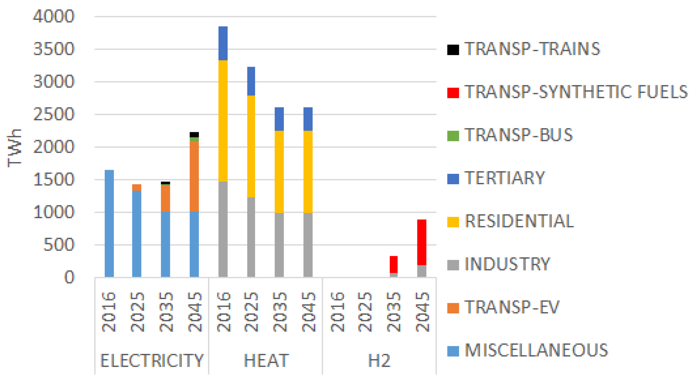
2.1.2. Energy System Modeling in Balmorel
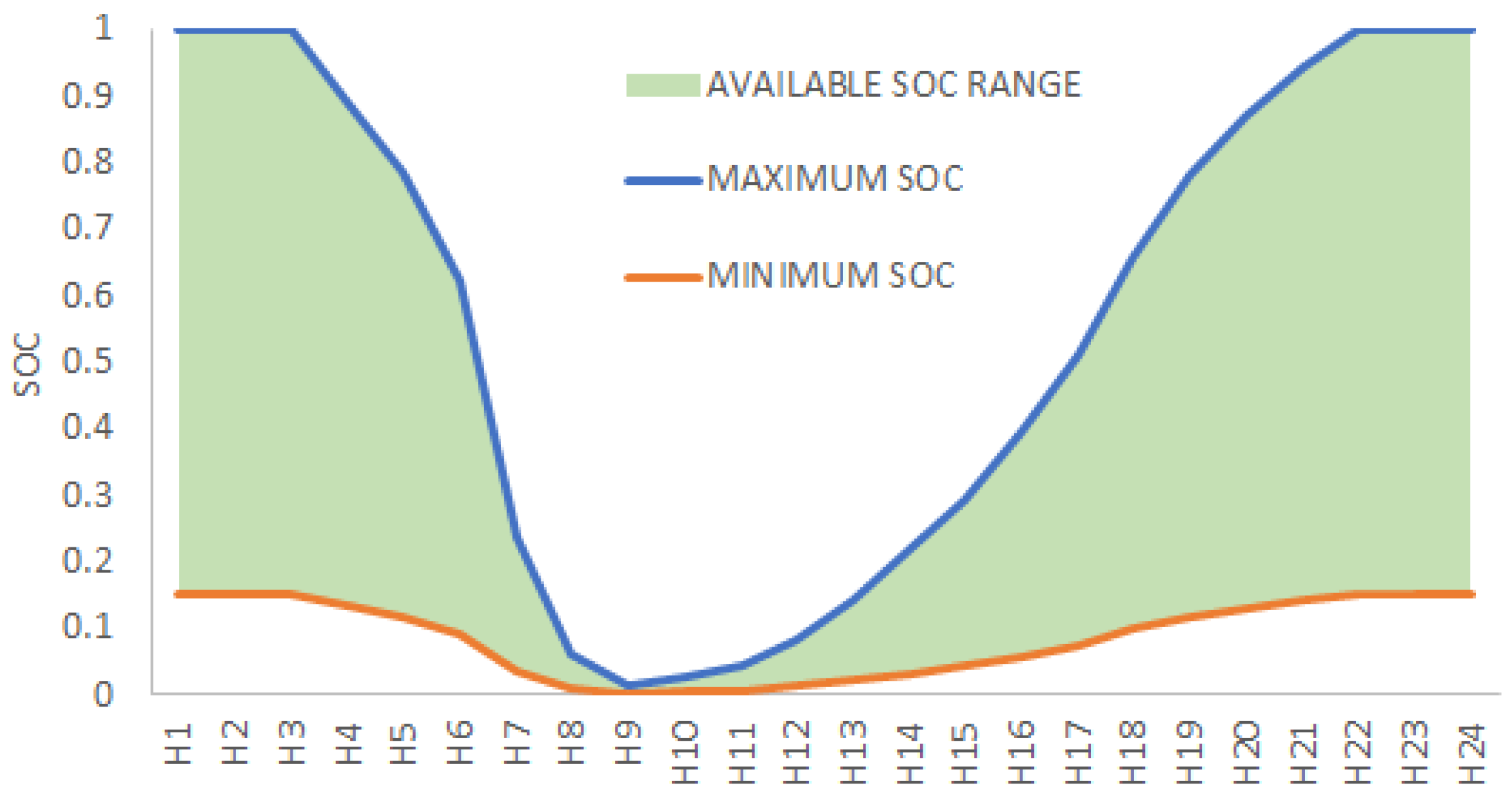
Storage and Generation Units
Electricity Network
Synthetic Gas
Transport Sector
Heat Sector
Energy Efficiency
Wind and Solar Modeling
Fuel Price and CO2 Tax
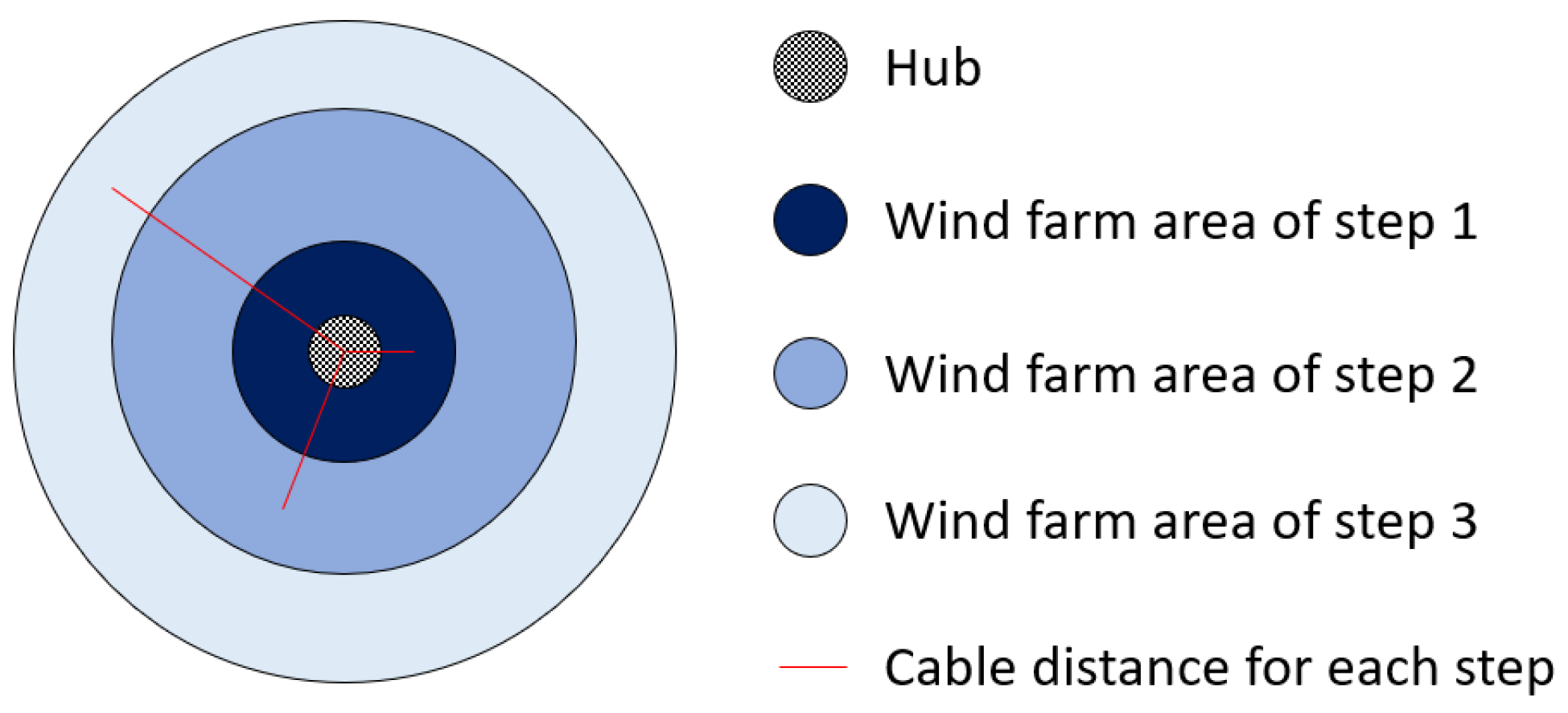
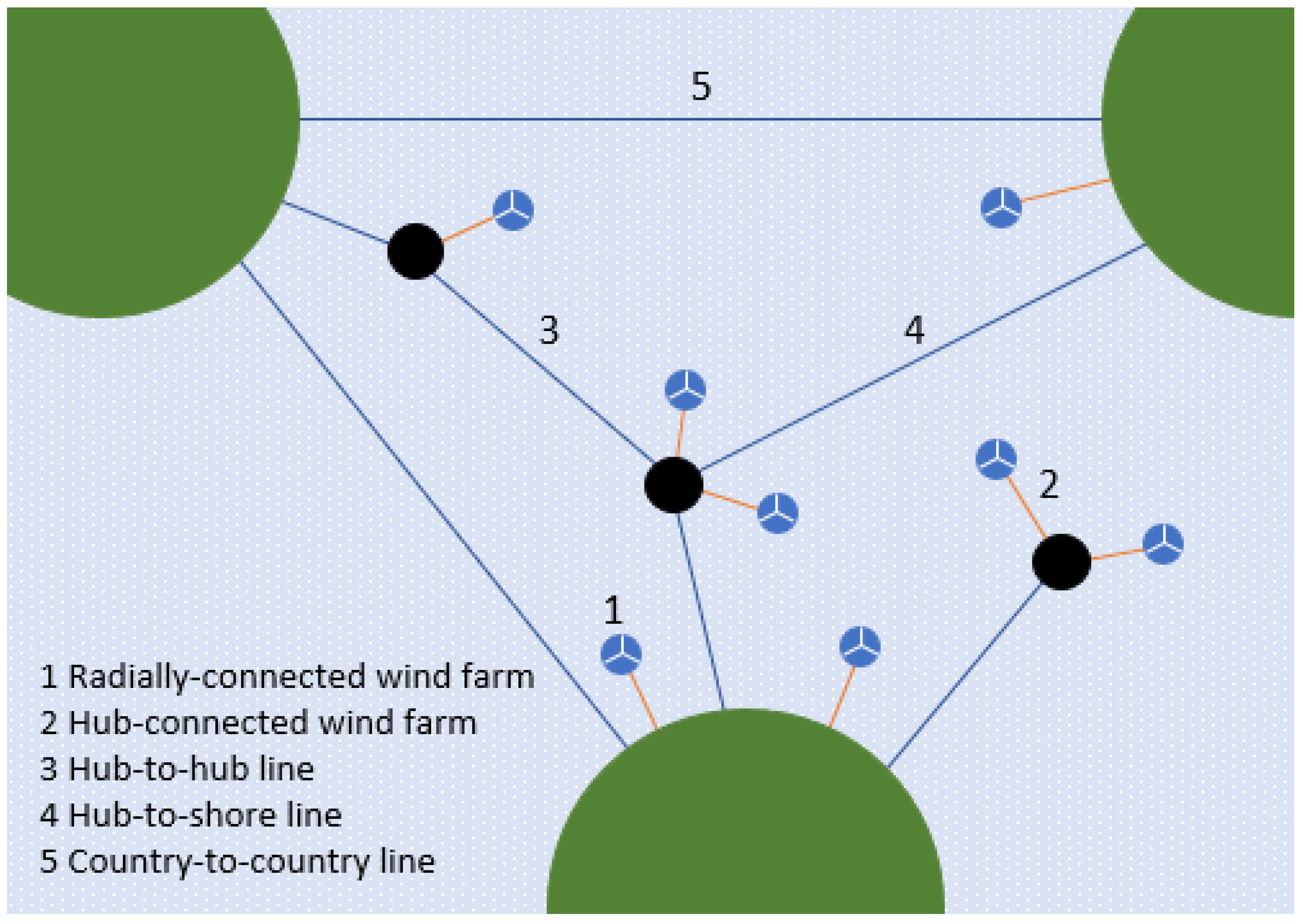
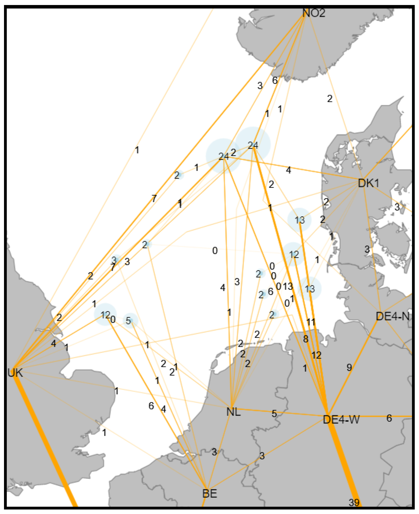
2.1.3. Offshore Grid Modeling
2.2. Large-Scale Hub-Connected Wind Farm Power Time Series Simulations
2.2.1. Wake Modeling
2.2.2. Large-Scale Hub-Connected Wind Generation Time Series
2.2.3. Modification of Large-Scale Hub-Connected Wind Generation Time Series
2.3. Optimization Approach
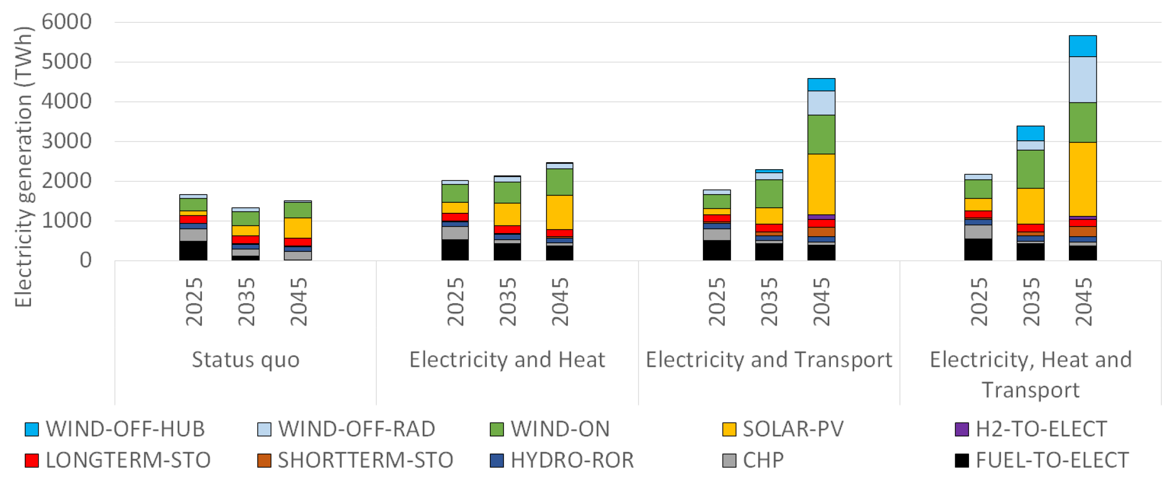
3. Scenarios
4. Results
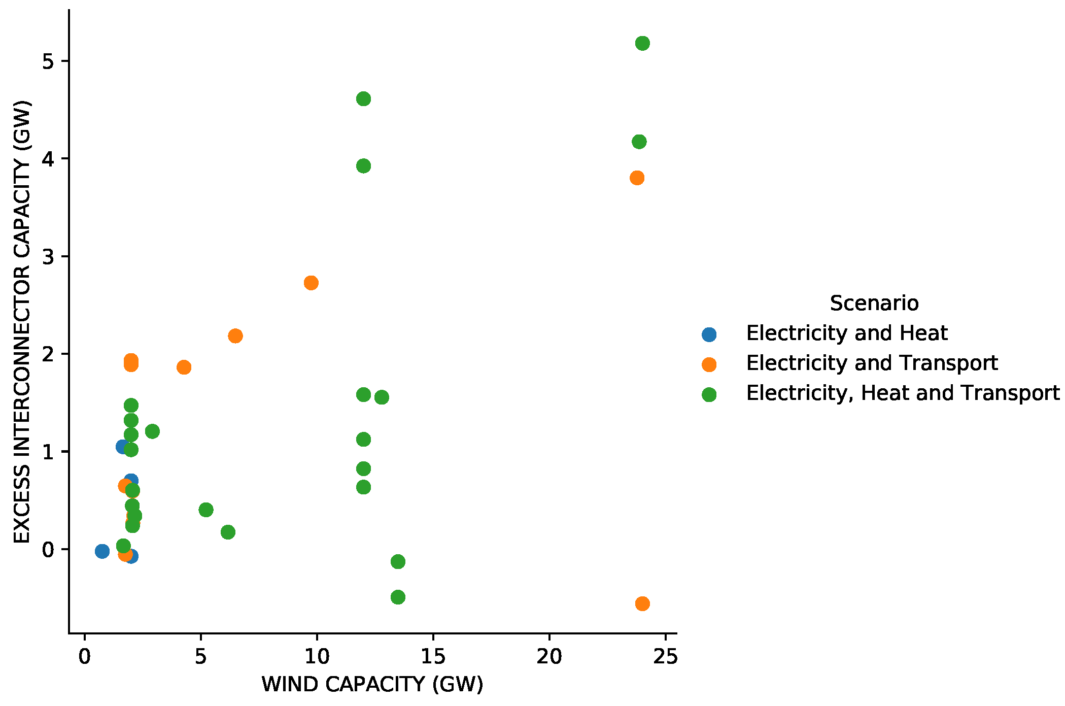
4.1. Sector Coupling Drives Offshore Grids
4.2. Sector Coupling Increases the Value of Offshore Grids
5. Discussion
6. Conclusions
Author Contributions
Funding
Institutional Review Board Statement
Informed Consent Statement
Data Availability Statement
Conflicts of Interest
Abbreviations
| VRE | variable renewable energy |
| PV | photovoltaic |
| H2 | hydrogen |
| EV | electric vehicle |
| SNG | synthetic natural gas |
References
- UNFCC. Adoption of the Paris Agreement; UNFCC: Bonn, Germany, 2015. [Google Scholar]
- Helgeson, B.; Peter, J. The role of electricity in decarbonizing European road transport—Development and assessment of an integrated multi-sectoral model. Appl. Energy 2020, 262, 114365. [Google Scholar] [CrossRef] [Green Version]
- Gea-Bermúdez, J.; Koivisto, M.; Münster, M. Optimization of the electricity and heating sectors development in the North Sea region towards 2050. In Proceedings of the 18th Wind Integration Workshop, Dublin, Ireland, 16–18 October 2019. [Google Scholar]
- Thellufsen, J.Z.; Lund, H. Cross-border versus cross-sector interconnectivity in renewable energy systems. Energy 2017, 124, 492–501. [Google Scholar] [CrossRef]
- Brown, T.; Schlachtberger, D.; Kies, A.; Schramm, S.; Greiner, M. Synergies of sector coupling and transmission reinforcement in a cost-optimised, highly renewable European energy system. Energy 2018, 160, 720–739. [Google Scholar] [CrossRef] [Green Version]
- Victoria, M.; Zhu, K.; Brown, T.; Andresen, G.B.; Greiner, M. The role of storage technologies throughout the decarbonisation of the sector-coupled European energy system. Energy Convers. Manag. 2019, 201, 111977. [Google Scholar] [CrossRef] [Green Version]
- Gea-Bermúdez, J.; Jensen, I.G.; Münster, M.; Koivisto, M.; Kirkerud, J.G.; Chen, Y.K.; Ravn, H. The role of sector coupling in the green transition: A least-cost energy system development in Northern-central Europe towards 2050. Appl. Energy 2021, 289, 116685. [Google Scholar] [CrossRef]
- The Global Wind Atlas. Global Wind Atlas; The Global Wind Atlas. 2021. Available online: https://globalwindatlas.info/ (accessed on 2 December 2021).
- Egelund, O.B. Wind Energy and Local Acceptance: How to Get Beyond the Nimby Effect. Eur. Energy Environ. Law Rev. 2010, 19, 239–251. [Google Scholar]
- The European Commission. EU Strategy on Offshore Renewable Energy; The European Commission: Brussels, Belgium, 2020. [Google Scholar]
- European Comission. Offshore Electricity Grid Infrastructure in Europe; European Comission: Brussels, Belgium, 2011. [Google Scholar]
- European Comission. Energy Infrastructure Priorities for 2020 and Beyond—A Blueprint for an Integrated European Energy Network; European Comission: Brussels, Belgium, 2011. [Google Scholar]
- The European Commission. Climate Strategies and Targets; The European Commission: Brussels, Belgium, 2020. [Google Scholar]
- Konstantelos, I.; Pudjianto, D.; Strbac, G.; De Decker, J.; Joseph, P.; Flament, A.; Kreutzkamp, P.; Genoese, F.; Rehfeldt, L.; Wallasch, A.K.; et al. Integrated North Sea grids: The costs, the benefits and their distribution between countries. Energy Policy 2017, 101, 28–41. [Google Scholar] [CrossRef]
- Koivisto, M.; Gea-Bermúdez, J.; Kanellas, P.; Das, K.; Sørensen, P. North Sea region energy system towards 2050: Integrated offshore grid and sector coupling drive offshore wind power installations. Wind Energy Sci. 2020, 5, 1705–1712. [Google Scholar] [CrossRef]
- Volker, P.J.H.; Hahmann, A.N.; Badger, J.; Jørgensen, H.E. Prospects for generating electricity by large onshore and offshore wind farms. Environ. Res. Lett. 2017, 12, 034022. [Google Scholar] [CrossRef]
- Agora Energiewende; Agora Verkehrswende; Technical University of Denmark; Max-Planck-Institute for Biogeochemistry. Making the Most of Offshore Wind: Re-Evaluating the Potential of Offshore Wind in the German North Sea; Technical Report; Agora Energiewende: Berlin, Germany, 2020. [Google Scholar]
- Holttinen, H.; Meibom, P.; Orths, A.; Lange, B.; O’Malley, M.; Tande, J.O.; Estanqueiro, A.; Gomez, E.; Söder, L.; Strbac, G.; et al. Impacts of large amounts of wind power on design and operation of power systems, results of IEA collaboration. Wind Energy 2011, 14, 179–192. [Google Scholar] [CrossRef]
- Murcia Leon, J.P.; Koivisto, M.J.; Sørensen, P.; Magnant, P. Power fluctuations in high-installation-density offshore wind fleets. Wind Energy Sci. 2021, 6, 461–476. [Google Scholar] [CrossRef]
- Van der Laan, M.; Hansen, K.S.; Sørensen, N.N.; Réthoré, P.E. Predicting wind farm wake interaction with RANS: An investigation of the Coriolis force. In Journal of Physics: Conference Series; IOP Publishing: Bristol, UK, 2015; Volume 625, p. 012026. [Google Scholar] [CrossRef]
- Nygaard, N.G.; Hansen, S.D. Wake effects between two neighbouring wind farms. In Journal of Physics: Conference Series; IOP Publishing: Bristol, UK, 2016; Volume 753, p. 032020. [Google Scholar] [CrossRef] [Green Version]
- Santos-Alamillos, F.; Thomaidis, N.; Usaola-García, J.; Ruiz-Arias, J.; Pozo-Vázquez, D. Exploring the mean-variance portfolio optimization approach for planning wind repowering actions in Spain. Renew. Energy 2017, 106, 335–342. [Google Scholar] [CrossRef]
- Koivisto, M.; Ekström, J.; Seppänen, J.; Mellin, I.; Millar, J.; Haarla, L. A statistical model for comparing future wind power scenarios with varying geographical distribution of installed generation capacity. Wind Energy 2016, 19, 665–679. [Google Scholar] [CrossRef]
- Wiese, F.; Bramstoft, R.; Koduvere, H.; Alonso, A.P.; Balyk, O.; Kirkerud, J.G.; Tveten, Å.G.; Bolkesjø, T.F.; Münster, M.; Ravn, H. Balmorel open source energy system model. Energy Strategy Rev. 2018, 20, 26–34. [Google Scholar] [CrossRef]
- Gea-Bermúdez, J.; Das, K.; Koivisto, M.J.; Koduvere, H. Day-ahead Market Modelling of Large-scale Highly-renewable Multi-energy Systems: Analysis of the North Sea Region towards 2050. Energies 2021, 14, 88. [Google Scholar] [CrossRef]
- Balmorel Community. Balmorel Code. Available online: https://github.com/balmorelcommunity/Balmorel (accessed on 2 December 2021).
- Balmorel Community. Balmorel Data. Available online: https://github.com/balmorelcommunity/Balmorel_data (accessed on 2 December 2021).
- Danish Energy Agency. Technology Catalogues; Danish Energy Agency: København, Denmark, 2020.
- Poncelet, K.; Delarue, E.; D’haeseleer, W. Unit commitment constraints in long-term planning models: Relevance, pitfalls and the role of assumptions on flexibility. Appl. Energy 2020, 258, 113843. [Google Scholar] [CrossRef]
- Koivisto, M.; Gea-Bermúdez, J.; Sørensen, P. North Sea offshore grid development: Combined optimization of grid and generation investments towards 2050. IET Renew. Power Gener. 2019, 14, 1259–1267. [Google Scholar] [CrossRef] [Green Version]
- EA Energy Analysis. Offshore Wind and Infrastructure; EA Energy Analysis: København, Denmark, 2020. [Google Scholar]
- EDMOnet-Bathymetry. EMODnet DTM. EDMOnet-Bathymetry: Europe 2021. Available online: https://www.emodnet-bathymetry.eu/ (accessed on 2 December 2021).
- Lazard’s Levelized Cost of Storage Analysis 3.0. Available online: https://www.lazard.com/media/450338/lazard-levelized-cost-of-storage-version-30.pdf (accessed on 2 December 2021).
- Gunkel, P.A.; Koduvere, H.; Kirkerud, J.G.; Fausto, F.J.; Ravn, H. Modelling transmission systems in energy system analysis: A comparative study. J. Environ. Manag. 2020, 262, 110289. [Google Scholar] [CrossRef]
- Nordic Energy Research; International Energy Agency. Nordic Energy Technology Perspectives 2016 Report; Nordic Energy Research: Oslo, Norway; International Energy Agency: Paris, France, 2016. [Google Scholar]
- Gea-Bermúdez, J.; Pade, L.L.; Koivisto, M.J.; Ravn, H. Optimal generation and transmission development of the North Sea region: Impact of grid architecture and planning horizon. Energy 2020, 191, 116512. [Google Scholar] [CrossRef]
- European Commission. A Clean Planet for All a European Long-Term Strategic Vision for a Prosperous, Modern, Competitive and Climate Neutral Economy; European Commission: Brussels, Belgium, 2018. [Google Scholar]
- Transport and Environment. How to Decarbonize the Transport Sector by 2050. Available online: https://www.transportenvironment.org/discover/how-decarbonise-european-transport-2050/ (accessed on 2 December 2021).
- Swisher, P. Modelling of Political and Technological Innovation on Northern Europe’s Energy System towards 2050. Master’s Thesis, Technical University of Denmark, Lyngby, Denmark, 2020. [Google Scholar]
- Gunkel, P.A.; Bergaentzlé, C.; Græsted Jensen, I.; Scheller, F. From passive to active: Flexibility from electric vehicles in the context of transmission system development. Appl. Energy 2020, 277, 115526. [Google Scholar] [CrossRef]
- Sims, R.E.; Mabee, W.; Saddler, J.N.; Taylor, M. An overview of second generation biofuel technologies. Bioresour. Technol. 2010, 101, 1570–1580. [Google Scholar] [CrossRef]
- Münster, M.; Morthorst, P.E.; Larsen, H.V.; Bregnbæk, L.; Werling, J.; Lindboe, H.H.; Ravn, H. The role of district heating in the future Danish energy system. Energy 2012, 48, 47–55. [Google Scholar] [CrossRef] [Green Version]
- Henning, H.M.; Palzer, A. A comprehensive model for the German electricity and heat sector in a future energy system with a dominant contribution from renewable energy technologies—Part I: Methodology. Renew. Sustain. Energy Rev. 2014, 30, 1003–1018. [Google Scholar] [CrossRef]
- Rehfeldt, M.; Fleiter, T.; Toro, F. A bottom-up estimation of the heating and cooling demand in European industry. Energy Effic. 2018, 11, 1057–1082. [Google Scholar] [CrossRef]
- Wiese, F.; Baldini, M. Conceptual model of the industry sector in an energy system model: A case study for Denmark. J. Clean. Prod. 2018, 203, 427–443. [Google Scholar] [CrossRef]
- Nuño, E.; Maule, P.; Hahmann, A.; Cutululis, N.; Sørensen, P.; Karagali, I. Simulation of transcontinental wind and solar PV generation time series. Renew. Energy 2018, 118, 425–436. [Google Scholar] [CrossRef] [Green Version]
- Koivisto, M.; Das, K.; Guo, F.; Sørensen, P.; Nuño, E.; Cutululis, N.; Maule, P. Using time series simulation tools for assessing the effects of variable renewable energy generation on power and energy systems. Wiley Interdiscip. Rev. Energy Environ. 2019, 8, e329. [Google Scholar] [CrossRef]
- Ruiz, P.; Nijs, W.; Tarvydas, D.; Sgobbi, A.; Zucker, A.; Pilli, R.; Jonsson, R.; Camia, A.; Thiel, C.; Hoyer-Klick, C.; et al. ENSPRESO—An open, EU-28 wide, transparent and coherent database of wind, solar and biomass energy potentials. Energy Strategy Rev. 2019, 26, 100379. [Google Scholar] [CrossRef]
- Koivisto, M.; Gea-Bermúdez, J. NSON-DK Energy System Scenarios, 2nd ed.; DTU Wind Energy: Roskilde, Denmark, 2018; Available online: https://orbit.dtu.dk/en/publications/nsondk-energy-system-scenarios--edition-2(a12307fd-b045-4d90-a745-38bca211b861).html (accessed on 2 December 2021).
- Flex4RES Project. Flexible Nordic Energy Systems Summary Report; Nordic Energy Research: Oslo, Norway, 2019. Available online: https://www.nordicenergy.org/wp-content/uploads/2019/07/Flex4RES_final_summary_report_aug2019.pdf (accessed on 2 December 2021).
- Negra, N.B.; Todorovic, J.; Ackermann, T. Loss evaluation of HVAC and HVDC transmission solutions for large offshore wind farms. Electr. Power Syst. Res. 2006, 76, 916–927. [Google Scholar] [CrossRef]
- Bastankhah, M.; Porté-Agel, F. A new analytical model for wind-turbine wakes. Renew. Energy 2014, 70, 116–123. [Google Scholar] [CrossRef]
- Wind Europe. Our Energy, Our Future. How Offshore Wind Will Help Europe Go Carbon-Neutral; Wind Europe: Brussels, Belgium, 2019. [Google Scholar]
- E3MLAB. PRIMES Model; E3MLAB: Athens, Greece, 2018. [Google Scholar]
- Victoria, M.; Haegel, N.; Peters, I.M.; Sinton, R.; Jäger-Waldau, A.; del Cañizo, C.; Breyer, C.; Stocks, M.; Blakers, A.; Kaizuka, I.; et al. Solar photovoltaics is ready to power a sustainable future. Joule 2021, 5, 1041–1056. [Google Scholar] [CrossRef]
- PROMOtion. WP 4.7 Deliverable: Preparation of Cost-Benefit Analysis from a Protection Point of View. PROMOtion Project 2020. Available online: https://www.promotion-offshore.net/ (accessed on 2 December 2021).
- Koivisto, M.; Maule, P.; Cutululis, N.; Sørensen, P. Effects of Wind Power Technology Development on Large-scale VRE Generation Variability. In Proceedings of the 2019 IEEE Milan PowerTech, Milan, Italy, 23–27 June 2019. [Google Scholar]
- IRENA. Renewable Power Generation Costs in 2018; IRENA: Abu Dhabi, United Arab Emirates, 2019. [Google Scholar]
- Department for Business, Energy and Industrial Strategy. Electricity Generation Costs 2020; Department for Business, Energy and Industrial Strategy: London, UK, 2020.
- Hevia-Koch, P.; Jacobsen, H. Comparing offshore and onshore wind development considering acceptance costs. Energy Policy 2019, 125, 9–19. [Google Scholar] [CrossRef]
- Langer, K.; Decker, T.; Roosen, J.; Menrad, K. A qualitative analysis to understand the acceptance of wind energy in Bavaria. Renew. Sustain. Energy Rev. 2016, 64, 248–259. [Google Scholar] [CrossRef]
- Jansen, M.; Staffell, I.; Kitzing, L.; Quoilin, S.; Wiggelinkhuizen, E.; Bulder, B.; Riepin, I.; Müsgens, F. Offshore wind competitiveness in mature markets without subsidy. Nat. Energy 2020, 5, 614–622. [Google Scholar] [CrossRef]


| Technology | 2025 | 2035 | 2045 | Source |
|---|---|---|---|---|
| Offshore wind radial (nearshore, AC, western Denmark) | 1.6609 | 1.5783 | 1.5140 | [28,30] [31,32] |
| Offshore wind radial (far offshore, AC, western Denmark) | 2.0662 | 1.8781 | 1.7379 | [28,30] [31,32] |
| Offshore wind radial (far offshore, DC, western Denmark) | 2.7208 | 2.4829 | 2.3139 | [28,30] [31,32] |
| Hub-connected offshore wind (20 m depth, step 1) | 2.0558 | 1.8420 | 1.7162 | [28,30] [31,32] |
| Hub-connected offshore wind (20 m depth, step 2) | 2.0872 | 1.8734 | 1.7475 | [28,30] [31,32] |
| Hub-connected offshore wind (20 m depth, step 3) | 2.1182 | 1.9044 | 1.7786 | [28,30] [31,32] |
| Hub-connected offshore wind (30 m depth, step 1) | 2.1658 | 1.9420 | 1.8062 | [28,30] [31,32] |
| Hub-connected offshore wind (30 m depth, step 2) | 2.1972 | 1.9734 | 1.8375 | [28,30] [31,32] |
| Hub-connected offshore wind (30 m depth, step 3) | 2.2282 | 2.0044 | 1.8686 | [28,30] [31,32] |
| Offshore hub (platform and equipment) | 0.1860 | 0.1860 | 0.1683 | [30] |
| Onshore wind | 1.2728 | 1.1456 | 1.0539 | [28] |
| Solar PV (AC side) | 0.4200 | 0.3000 | 0.2600 | [28] |
| Gas turbine (electricity only) | 0.5015 | 0.4760 | 0.4590 | [28] |
| Heat pump (ground to water) | 0.6580 | 0.5922 | 0.5626 | [28] |
| Electrolyser (alkaline) | 0.6500 | 0.4500 | 0.3000 | [28] |
| Electrolyser (alkaline, connected to district heating) | 0.6605 | 0.4605 | 0.3105 | [28] |
| Fuel cell (solid oxide) | 1.5000 | 0.8000 | 0.6500 | [28] |
| Lithium battery (electricity storage) | 0.4105 | 0.3284 | 0.2463 | [33] |
| Pumped hydro (electricity storage) | 0.2908 | 0.2908 | 0.2908 | [28] |
| Steel tank (H2 storage) | 0.0570 | 0.0450 | 0.0270 | [28] |
| Water tank (Heat storage) | 0.0030 | 0.0030 | 0.0030 | [28] |
| Pit (heat storage, central) | 0.0015 | 0.0014 | 0.0013 | [28] |
| Pit (heat storage, decentral) | 0.0005 | 0.0004 | 0.0004 | [28] |
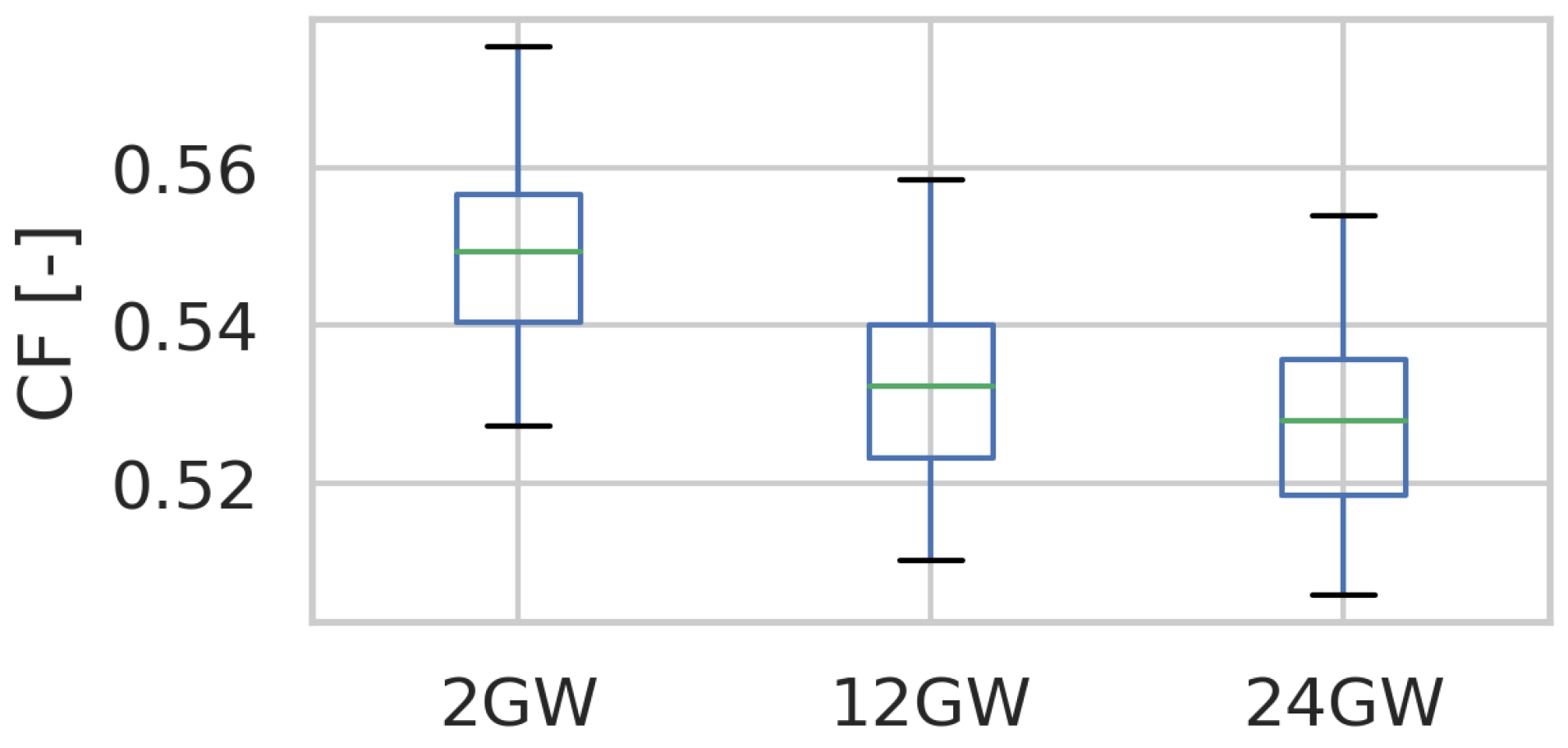
| Time Series | 2 GW | 12 GW | 24 GW |
|---|---|---|---|
| Without wake loss modeling | 59.7% | 59.7% | 59.7% |
| With wake loss modeling, non-modified | 54.1% | 52.4% | 51.9% |
| With wake loss modeling, modified | 54.1% | 52.0% | 51.5% |
| Scenario | Investments in Electric Power-to-Heat Units | Decarbonization of the Transport Sector |
|---|---|---|
| Status quo | - | - |
| Electricity and Heat | + | - |
| Electricity and Transport | - | + |
| Electricity, Heat and Transport | + | + |
| Sectors Coupled | All Studied Countries in 2045 | North Sea Region in 2045 | |||||
|---|---|---|---|---|---|---|---|
| Electricity Demand (TWh) | Installed Offshore Wind Capacity (GW) | Share of Offshore Wind in Electricity Demand (%) | Installed Offshore Wind Capacity (GW) | Hub-Connected Capacity Share (%) | Interconnectors (TWkm) | Share of Hub-Connected Interconnectors (%) | |
| Status quo | 1491 | 12 | 3 | 8 | 0 | 6 | 0 |
| Electricity and Heat | 2432 | 38 | 6 | 22 | 28 | 15 | 8 |
| Electricity and Transport | 4331 | 203 | 21 | 148 | 86 | 38 | 72 |
| Electricity, Heat and Transport | 5408 | 378 | 31 | 255 | 84 | 50 | 81 |
| Sectors Coupled | Time Period | Difference in Capital Expenditure (b€2016/year) | Difference in Operational Expenditure (b€2016/year) | Total System Cost Difference (b€2016/year) | Relative Change with Respect to Total System Cost (%) |
|---|---|---|---|---|---|
| Electricity and Heat | 2020–2030 | −0.02 | 0.02 | 0.00 | 0.00 |
| 2030–2040 | 0.18 | −0.17 | 0.00 | 0.00 | |
| 2040–2050 | 0.15 | −0.16 | −0.01 | −0.01 | |
| Electricity and Transport | 2020–2030 | 0.04 | −0.03 | 0.01 | 0.01 |
| 2030–2040 | 0.38 | −0.36 | 0.02 | 0.01 | |
| 2040–2050 | −0.09 | −0.73 | −0.82 | −0.29 | |
| Electricity, Heat and Transport | 2020–2030 | −0.07 | 0.07 | 0.00 | 0.00 |
| 2030–2040 | 1.35 | −2.28 | −0.93 | −0.63 | |
| 2040–2050 | −2.34 | 0.76 | −1.57 | −0.71 |
Publisher’s Note: MDPI stays neutral with regard to jurisdictional claims in published maps and institutional affiliations. |
© 2022 by the authors. Licensee MDPI, Basel, Switzerland. This article is an open access article distributed under the terms and conditions of the Creative Commons Attribution (CC BY) license (https://creativecommons.org/licenses/by/4.0/).
Share and Cite
Gea-Bermúdez, J.; Kitzing, L.; Koivisto, M.; Das, K.; Murcia León, J.P.; Sørensen, P. The Value of Sector Coupling for the Development of Offshore Power Grids. Energies 2022, 15, 747. https://doi.org/10.3390/en15030747
Gea-Bermúdez J, Kitzing L, Koivisto M, Das K, Murcia León JP, Sørensen P. The Value of Sector Coupling for the Development of Offshore Power Grids. Energies. 2022; 15(3):747. https://doi.org/10.3390/en15030747
Chicago/Turabian StyleGea-Bermúdez, Juan, Lena Kitzing, Matti Koivisto, Kaushik Das, Juan Pablo Murcia León, and Poul Sørensen. 2022. "The Value of Sector Coupling for the Development of Offshore Power Grids" Energies 15, no. 3: 747. https://doi.org/10.3390/en15030747
APA StyleGea-Bermúdez, J., Kitzing, L., Koivisto, M., Das, K., Murcia León, J. P., & Sørensen, P. (2022). The Value of Sector Coupling for the Development of Offshore Power Grids. Energies, 15(3), 747. https://doi.org/10.3390/en15030747