Power Flows and Losses Calculation in Radial Networks by Representing the Network Topology in the Hierarchical Structure Form

Abstract

This paper proposes a structured hierarchical-multilevel approach to calculating the power flows and losses of electricity in radial electrical networks with different nominal voltages at given loads and voltages of the power source. The researched electrical networks are characterized by high dimensionality, dynamism of development, but also insufficient completeness and reliability of state information. The approach is based on the representation of the initial network graph in the form of a hierarchical-multilevel structure, divided into two stages with rated voltages $U_{nom}\le 35$ kV and $U_{nom}\ge 35$ kV, and using the traditional (manual) engineering two-stage method, where the calculation is performed in a sequence from bottom to top (stage 1) and from top to bottom (stage 2), moving along the structure of the network. The application of the above approach makes it possible to obtain an algorithm for implementation on a computer, which is characterized by universality (for an arbitrary configuration and complexity of the network), high performance and low requirements for the computer memory.

1. Introduction

It is well known that electricity losses in electrical grids of power systems consist of the following components:

• Technological factor—it directly depends on the characteristic physical processes, and can change under the influence of the load component, conditionally fixed costs, as well as climatic conditions;
• Energy costs spent on the operation of auxiliary equipment and ensuring the necessary conditions for the work of technical personnel;
• Commercial losses—this category includes errors in metering devices, as well as other factors that cause the underestimation of electric energy.

When determining electrical energy losses in electrical networks of power systems, the greatest interest, from the point of view of the specific contribution to the total amount of losses, structural complexity and complexity of the calculation, are the load losses in the lines and power transformers of the network [1,2,3,4,5,6].

A significant part of electricity is transmitted through highly branched distribution networks of 6–20 kV, which mainly operate as a radial network. These networks are characterized by high dimension, dynamism of development, insufficient completeness and reliability of state information [7,8,9]. The magnitude of losses in these networks can reach up to 70% of the total electrical energy losses; therefore, an objective estimation of electricity losses in the considered electrical networks is extremely important.

The features of the calculating electricity losses tasks in radial electric networks with nominal voltage $U_{nom}\ge 35$ kV include: considering the reactive power $Q_C$ of the power lines; considering corona losses $\Delta P_{cor}$ in overhead lines; considering power losses $\Delta \underline{S}$ in network elements; considering the longitudinal $\Delta U$ and transverse $\delta U$ components of the voltage drop in the network elements, calculated according to the actual voltage U of the network, and not according to the nominal $U_{nom}$ [10]. Distribution networks with $U_{nom}\ge 35$ kV are similar in configuration to networks of 6–20 kV; from the point of view of sate information, they are sufficiently provided and they are more adjacent to multi-circuit electrical networks [11]. These specific features of $U_{nom}\ge 35$ kV networks indicate that, in order to determine electricity losses, it is necessary to calculate power flows, i.e., determine the unknown voltages in nodes, flows and power losses in network elements (power lines and transformers) [12,13,14,15,16,17,18,19]. These power flow calculations [11,20,21] are performed, as a rule, at a given voltage of the power supply and constant values of the loads on the low-voltage side of step-down consumer substations (this is the way of specifying the initial information that most closely matches the operating conditions and is typical for the electrical networks under consideration).

To solve such problems, it is important to develop universal and efficient algorithmic methods from the point of view of implementation and computation complexity.

Therefore, in [2,6,22], a structured hierarchical-multilevel approach was applied when solving the following problems:

• Element-by-element calculation of load electricity losses in distribution electric networks 6–20 kV;
• Calculation of power flows and losses of electricity in radial electrical networks of 35 kV and above, at given loads and voltage of the power source;
• Problems of designing a system for electrical distribution networks’ overhead lines wire breakage remote diagnostics.

The use of this approach made it possible to obtain a universal (for an arbitrary configuration and network complexity) and efficient (in terms of the number of computational operations and the amount of computer memory consumed) algorithm.

In this paper, the described approach was used to calculate the power flows and losses of electricity in radial circuits with different nominal voltages at given loads and voltage of the power source. The advantage of this approach is that the use of the apparatus of computing Petri nets for its implementation makes it possible to build a self-organizing multicomponent computational algorithm, convenient from the point of view of implementation on a computer, modification and interpretation, as well as from the point of view of the organization of parallel-sequential computations in order to increase the computing speed.

A distribution network with n nodes and m network elements (power lines and transformers) with a tree structure is considered, which contains transformers connecting subnets with different nominal voltages. The specified parameters are: network scheme; loads powers; resistances and conductivities of elements; power source voltage and nominal sub-network voltages. The unknown parameters are: unknown voltages at nodes, flows and power losses at elements, power losses in the network as a whole.

2. Structural Network Model

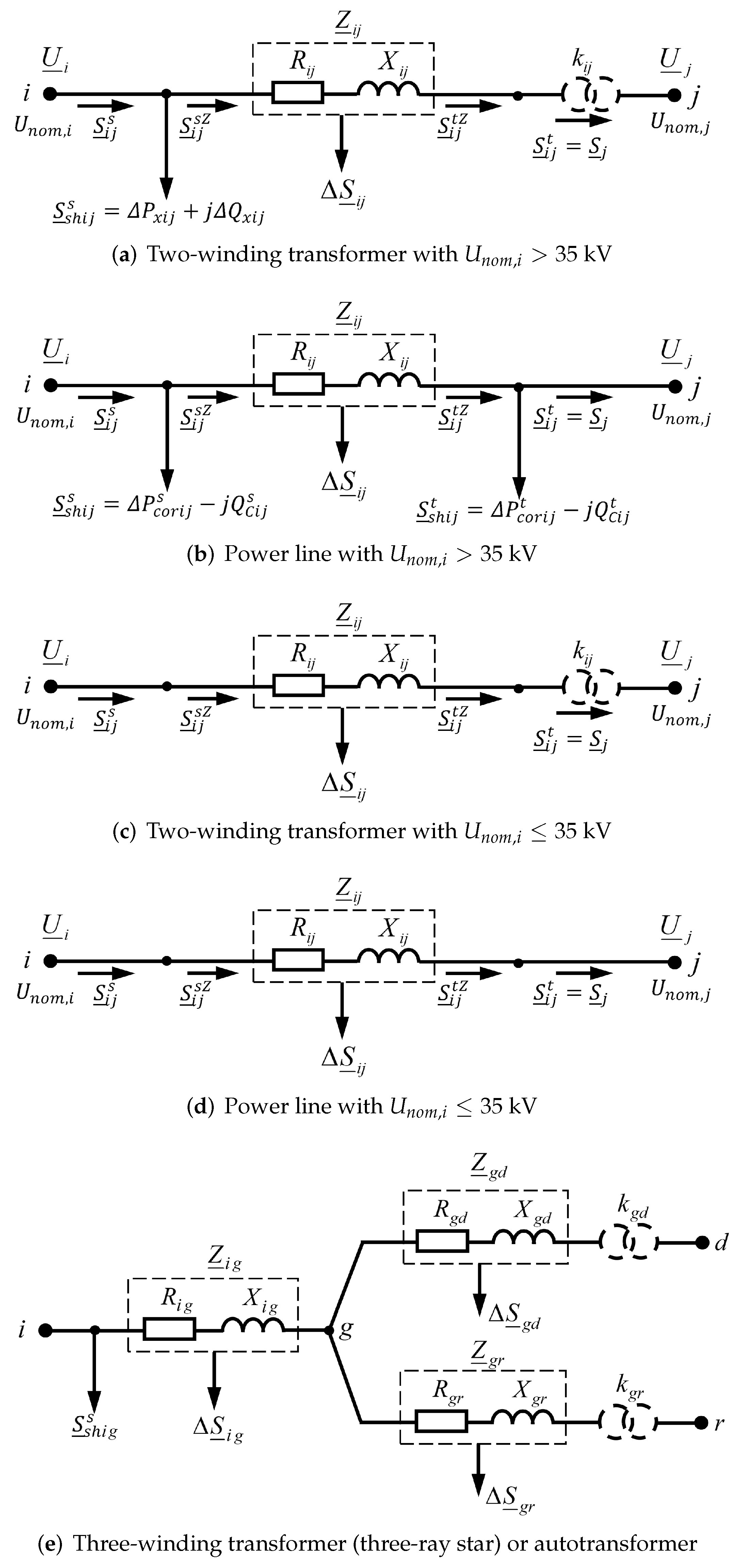
The scheme of a radial electric network with different nominal voltages is represented in the form of an oriented graph $(L,\Gamma )$ with a tree structure (see Figure 1), where L is a set of network nodes (graph vertices); $\Gamma$ is a mapping of the set L to L, showing how the nodes of the network from the set L are connected to each other, meaning that:

$$\begin{array}{c}\Gamma :L\to L,\Gamma \left(i\right)\subset L,\forall i\in L\backslash L_0,\end{array}$$

(1)

$$\begin{array}{c}\Gamma \subseteq L\times L,{\Gamma }_i=\left\{i\right\}\times \Gamma \left(i\right),\forall i\in L\backslash L_0,\end{array}$$

(2)

$$\begin{array}{c}\Gamma =\bigcup _{i\in L\backslash L_0}{\Gamma }_i,L\backslash \left\{0\right\}=\bigcup _{i\in L\backslash L_0}\Gamma \left(i\right),L_0\subset L,\end{array}$$

(3)

$$\begin{array}{c}\Gamma \left(i\right)=\varnothing ,{\Gamma }_i=\varnothing ,\forall i\in L_0,\end{array}$$

(4)

where $L_0$—the set of end vertices of the $(L,\Gamma )$ graph, i.e., end (load) network nodes; $L\backslash L_0$—set of intermediate graph vertices $(L,\Gamma )$, including $i=0$ vertex, i.e., including power supply node; $\Gamma \left(i\right)$—set of end vertices of edges, which source vertex is a vertex $i\in L\backslash L_0$; ${\Gamma }_i$—set of edges $(i,j)$, which source vertex is vertex $i\in L\backslash L_0$.

A set $L_Y$ is introduced, the elements of which are the numbers of subgraphs’ internal nodes (three-ray stars) corresponding to three-winding transformers or autotransformers of the electrical network (here, an internal node is a node connecting all three rays of a subgraph).

Each vertex $i\in L$ of the graph $(L,\Gamma )$ of the network is associated with a nominal voltage $U_{nom,i}$. The elements of the sets $L_Y$ and $\left\{U_{nom,i}\mid i\in L\right\}$ serve as signs for the choice of the equivalent circuit and the corresponding calculation formula for each element $(i,j)\in \Gamma$ when calculating the power flows and losses of electricity in the network.

Figure 2 shows equivalent circuits of network elements with different nominal voltages [11,21]:

(a)

Equivalent circuit of a two-winding transformer with $U_{nom,i}>35$ kV;

(b)

Equivalent circuit of a power line with $U_{nom,i}>35$ kV;

(c)

Equivalent circuit of a two-winding transformer with $U_{nom,i}\le 35$ kV;

(d)

Equivalent circuit of a power line with $U_{nom,i}\le 35$ kV;

(e)

Equivalent circuit of a three-winding transformer (three-ray star) or autotransformer, where $(l,g)$ corresponds the primary voltage winding; $(g,d)$, $(g,r)$—secondary voltage winding; g—inner node of a three-pointed star connecting the $(l,g)$, $(g,d)$, $(g,r)$.

Note that the equivalent circuit of the edge $(l,g)$ is similar to the equivalent circuit of (a) without an ideal transformer, and the equivalent circuits of the edges $(g,d)$, $(g,r)$ are identical with the equivalent circuit (c).

In Figure 2, the following designations are adopted: ${\underline{S}}_{ij}^s,{\underline{S}}_{ij}^t$—power flows, respectively, at the beginning and at the end of the section (source and target, respectively) $(i,j)\in \Gamma$; ${\underline{S}}_{ij}^{sZ}$,${\underline{S}}_{ij}^{tZ}$—power flows, respectively, at the beginning and at the end of the resistance ${\underline{Z}}_{ij}$ of Section $(i,j)\in \Gamma$; ${\underline{S}}_j$—power flowing through a node $j\in L$ (since the power flows are directed from the power supply node $i=0$ to the set of load nodes $L_0$, as can be seen in Figure 1), then, ${\underline{S}}_{ij}^t={\underline{S}}_j$, ($\forall (i,j)\in \Gamma$); ${\underline{U}}_i,{\underline{U}}_j$—node stresses, respectively, at the beginning and at the end of Section $(i,j)\in \Gamma$; ${\underline{S}}_{shij}^s,{\underline{S}}_{shij}^t$—power flows (losses) in shunts, i.e., in transverse branches, respectively, at the beginning and at the end of Section $(i,j)\in \Gamma$; $\Delta {\underline{S}}_{ij}$—power loss in resistance ${\underline{Z}}_{ij}$; $\Delta P_{xij}$—active power losses in the steel of the transformer for magnetization reversal (hysteresis) and eddy currents; $\Delta Q_{xij}$—losses of reactive power in the steel of the transformer for its magnetization; $\Delta P_{corij}$—active corona power losses (or in isolation); $Q_{Cij}$—charging shunt power; $k_{ij}$—transformation ratio.

Furthermore, to calculate the above parameters of the power flow, the following parameters of the network elements are used: $R_{ij}$, $X_{ij}$—respectively, the active and reactive resistances of the longitudinal branch of Section $(i,j)\in \Gamma$; $q_{ij}$, $b_{ij}$—respectively, the active and reactive conductivity in the transverse branches of Section $(i,j)\in \Gamma$.

The procedure for choosing an equivalent circuit and the corresponding calculation formula for each Section $(i,j)\in \Gamma$ when calculating the power flows and losses of electricity in the network is described using the predicate functions given in

Table 1. Predicate functions for choosing the equivalent circuit and calculation formula for each Section $(i,j)\in \Gamma$ of the network.

Section Type Number (p)	Predicate Functions for Choosing the Equivalent Circuit and Calculation Formula for Each Section $(\mathit{i},\mathit{j})\in \mathbf{\Gamma }$	Equivalent Schemes: Figure 2	Operators for Calculating Power Flows ${\mathit{F}}_{\mathit{S}}^{(\cdot )}\left(\mathit{\dots }\right)$ and Voltages ${\mathit{F}}_{\mathit{U}}^{(\cdot )}\left(\mathit{\dots }\right)$ in the Network Nodes
1	$(j\notin L_Y)\wedge (U_{nom.i}>35kV)\wedge (U_{nom,i}>U_{nom,j})$	(a)	$F_S^{\left(1\right)}(\dots )$$F_U^{\left(1\right)}(\dots )$
2	$(j\notin L_Y)\wedge (U_{nom,i}>35kV)\wedge (U_{nom,i}=U_{nom,j})$	(b)	$F_S^{\left(2\right)}(\dots )$$F_U^{\left(2\right)}(\dots )$
3	$(j\notin L_Y)\wedge (U_{nom,i}\le 35kV)\wedge (U_{nom,i}>U_{nom,j})$	(c)	$F_S^{\left(3\right)}(\dots )$$F_U^{\left(1\right)}(\dots )$
4	$(j\notin L_Y)\wedge (U_{nom,i}\le 35kV)\wedge (U_{nom,i}=U_{nom,j})$	(d)	$F_S^{\left(4\right)}(\dots )$$F_U^{\left(2\right)}(\dots )$
5	$(j\in L_Y)\wedge (U_{nom,i}>35kV)\wedge (U_{nom,i}=U_{nom,j})$	(e), where $i=l$, $j=q$	$F_S^{\left(5\right)}(\dots )$$F_U^{\left(2\right)}(\dots )$
6	$(i\in L_Y)\wedge (U_{nom,i}>35kV)\wedge (U_{nom,i}>U_{nom,j})$	(e), where $i=g$, $j=d \text{or} r$	$F_S^{\left(3\right)}(\dots )$$F_U^{\left(1\right)}(\dots )$

.

In Table 1: $F_S^{\left(p\right)}(\dots )$—operators for calculating power flows (S) of Section $(i,j)$, type p; and $F_U^{\left(p\right)}(\dots )$—operators for calculating voltages (U) in nodes at the ends of sections $(i,j)$, type p.

The following is an example of the formation of computational sets for the original network topology in Figure 1. For the directed network graph shown in Figure 1: $L=\left\{0,1,2,\dots ,45\right\}$; $L_0=\left\{1,2,3,\dots ,15\right\}$; $L\backslash L_0=\left\{0,16,\dots ,44\right\}$; sets $\Gamma \left(i\right)$, ${\Gamma }_i$, $\forall i\in L\backslash L_0$ from (1) to (4), corresponding to this example are given in

Table 2. Sets $\Gamma \left(i\right)$ and ${\Gamma }_i$, $\forall i\in L\backslash L_0$.

	Sets $\mathbf{\Gamma }\left(\mathit{i}\right)$ $\forall \mathit{i}\in \mathit{L}\cdot {\mathit{L}}_0$	Sets ${\mathbf{\Gamma }}_{\mathit{i}}$ $\forall \mathit{i}\in \mathit{L}\cdot {\mathit{L}}_0$
1	$\Gamma \left(0\right)=\left\{44\right\}$	${\Gamma }_0=\left\{(0,44)\right\}$
2	$\Gamma \left(16\right)=\left\{1\right\}$	${\Gamma }_{16}=\left\{(16,1)\right\}$
3	$\Gamma \left(17\right)=\left\{16,18\right\}$	${\Gamma }_{17}=\left\{(17,16),(17,18)\right\}$
4	$\Gamma \left(18\right)=\left\{19\right\}$	${\Gamma }_{18}=\left\{(18,19)\right\}$
5	$\Gamma \left(19\right)=\left\{2\right\}$	${\Gamma }_{19}=\left\{(19,2)\right\}$
6	$\Gamma \left(20\right)=\left\{21\right\}$	${\Gamma }_{20}=\left\{(20,21)\right\}$
7	$\Gamma \left(21\right)=\left\{7,22\right\}$	${\Gamma }_{21}=\left\{(21,7),(21,22)\right\}$
8	$\Gamma \left(22\right)=\left\{23,24\right\}$	${\Gamma }_{22}=\left\{(22,23),(22,24)\right\}$
9	$\Gamma \left(23\right)=\left\{25,45\right\}$	${\Gamma }_{23}=\left\{(23,25),(23,45)\right\}$
10	$\Gamma \left(24\right)=\left\{6,26\right\}$	${\Gamma }_{24}=\left\{(24,6),(24,26)\right\}$
11	$\Gamma \left(25\right)=\left\{4\right\}$	${\Gamma }_{25}=\left\{(25,4)\right\}$
12	$\Gamma \left(26\right)=\left\{5\right\}$	${\Gamma }_{26}=\left\{(26,5)\right\}$
13	$\Gamma \left(27\right)=\left\{20,28,29\right\}$	${\Gamma }_{27}=\left\{(27,20),(27,28),(27,29)\right\}$
14	$\Gamma \left(28\right)=\left\{30\right\}$	${\Gamma }_{28}=\left\{(28,30)\right\}$
15	$\Gamma \left(29\right)=\left\{31\right\}$	${\Gamma }_{29}=\left\{(29,31)\right\}$
16	$\Gamma \left(30\right)=\left\{32\right\}$	${\Gamma }_{30}=\left\{(30,32)\right\}$
17	$\Gamma \left(31\right)=\left\{33\right\}$	${\Gamma }_{31}=\left\{(31,33)\right\}$
18	$\Gamma \left(32\right)=\left\{8\right\}$	${\Gamma }_{32}=\left\{(32,8)\right\}$
19	$\Gamma \left(33\right)=\left\{34,35\right\}$	${\Gamma }_{33}=\left\{(33,34),(33,35)\right\}$
20	$\Gamma \left(34\right)=\left\{9\right\}$	${\Gamma }_{34}=\left\{(34,9)\right\}$
21	$\Gamma \left(35\right)=\left\{10\right\}$	${\Gamma }_{35}=\left\{(35,10)\right\}$
22	$\Gamma \left(36\right)=\left\{37\right\}$	${\Gamma }_{36}=\left\{(36,37)\right\}$
23	$\Gamma \left(37\right)=\left\{15,38\right\}$	${\Gamma }_{37}=\left\{(37,15),(37,38)\right\}$
24	$\Gamma \left(38\right)=\left\{39,40\right\}$	${\Gamma }_{38}=\left\{(38,39),(38,40)\right\}$
25	$\Gamma \left(39\right)=\left\{11\right\}$	${\Gamma }_{39}=\left\{(39,11)\right\}$
26	$\Gamma \left(40\right)=\left\{14,41\right\}$	${\Gamma }_{40}=\left\{(40,14),(40,41)\right\}$
27	$\Gamma \left(41\right)=\left\{42,43\right\}$	${\Gamma }_{41}=\left\{(41,42),(41,43)\right\}$
28	$\Gamma \left(42\right)=\left\{12\right\}$	${\Gamma }_{42}=\left\{(42,12)\right\}$
29	$\Gamma \left(43\right)=\left\{13\right\}$	${\Gamma }_{43}=\left\{(43,13)\right\}$
30	$\Gamma \left(44\right)=\left\{17,27,36\right\}$	${\Gamma }_{44}=\left\{(44,17),(44,27),(44,36)\right\}$
31	$\Gamma \left(45\right)=\left\{3\right\}$	${\Gamma }_{45}=\left\{(45,3)\right\}$

; the edges set $\Gamma$ is obtained using Formula (), i.e., the union of sets ${\Gamma }_i$, $\forall i\in L\backslash L_0$ (see Table 2).

In the considered graph of the electrical network, the following is shown:

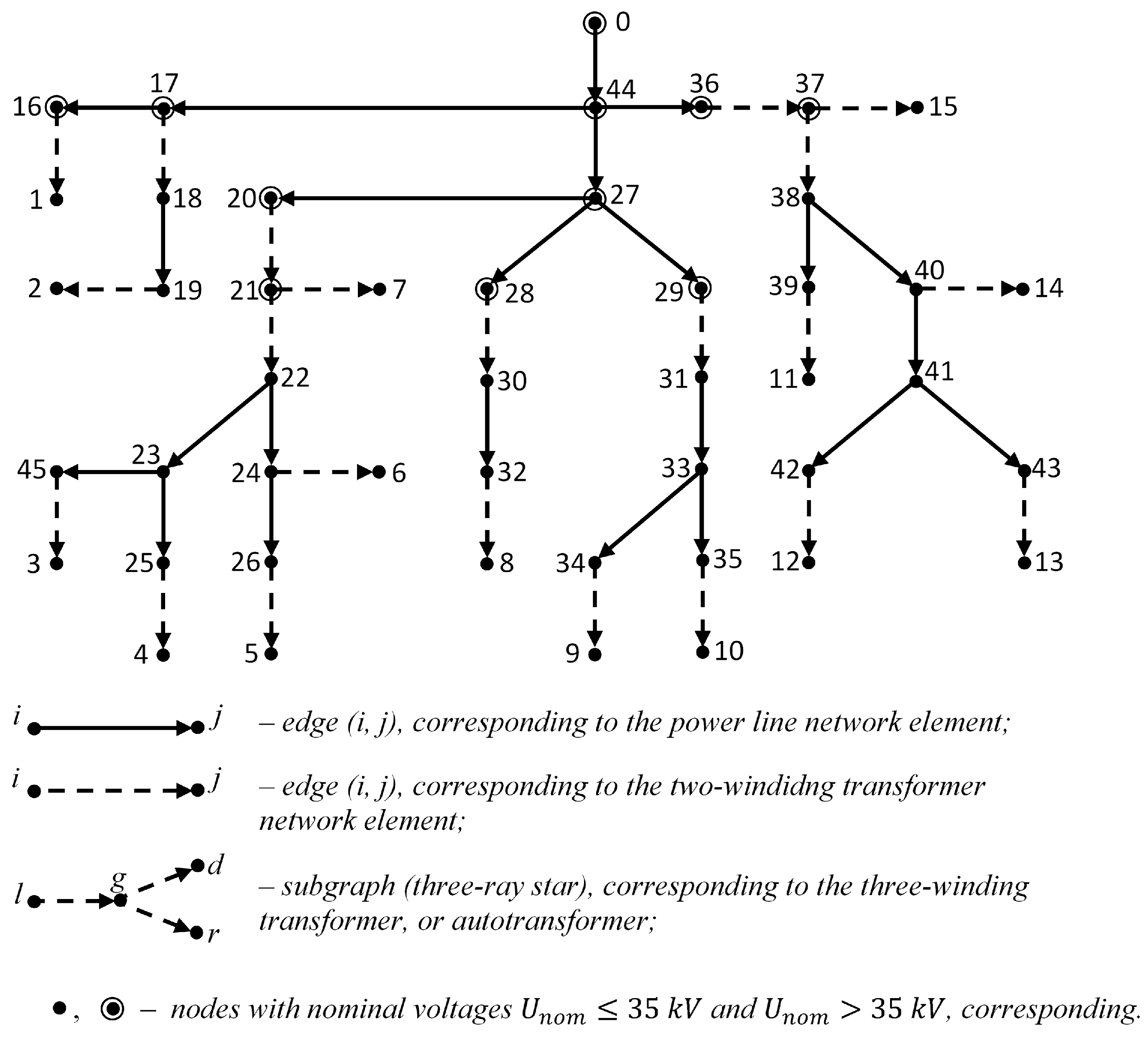
• All end sections of the network are double-winding transformers, the end nodes of which form a set of load nodes $L_0$;
• At sections (17, 18), (28, 30), (29, 31), two-winding communication transformers are installed between network lines of different rated voltage;
• Two three-winding communication transformers are installed between the lines of the network of different rated voltages: the first corresponds to a three-ray star from three sections (20, 21), (21, 7), (21, 22) with an internal node $g=21$; the second—to a three-rayed star, consisting of three sections (36, 37), (37, 15), (37, 38) with an internal node $g=37$. Here, sections (20, 21), (36, 37) correspond to the primary windings, and sections (21, 7), (21, 22) and (37, 15), (37, 38)—to the secondary windings of a three-winding coupling transformer;
• Communication transformers divide the initial network graph into two subgraphs: a subgraph with a lower step of the rated voltage $U_{nom}\le 35$ kV, whose nodes are shown as a point “⋅”; subgraph with the upper step of the rated voltage $U_{nom}>35$ kV, which nodes are shown as a point with a circle.

The set of internal nodes of three-winding coupling transformers has the form $L_Y=\left\{21,37\right\}$.

3. Calculation Algorithm Formulation and Discussion

3.1. Description of a Structured Hierarchically Multilevel Approach to the Calculation of Power Flows and Losses of Electricity in Radial Networks with Different Rated Voltages

To calculate the power flows and losses of electricity in radial electrical networks with different rated voltages, a two-stage method is used: in the first stage (from bottom to top), the flows and power losses in lines and transformers (autotransformers) are determined from loads to the power source; at the second stage, in the reverse order (from bottom to top), the voltages $U_i$ for nodes $i\in L_0$ are calculated from the power supply to the loads.

Unlike [2,6,22], this work considers electrical networks with different nominal voltages, i.e., networks with two subnets: a subnetwork with nominal voltage $U_{nom}\le 35$ kV and a subnetwork with $U_{nom}>35$ kV. To calculate the power flow of subnet with $U_{nom}>35$ kV a two-stage iterative method is used [11,21], where the “bottom–up” and “top–down” stages are repeated until the required calculation accuracy is obtained. To calculate the power flow of subnet with $U_{nom}\le 35$ kV—a two-stage method is used with one pass of the “bottom–up” and “top–down” stages.

To establish and organize such a sequence of calculations, the initial graph is represented in the form of a hierarchically multilevel structure.

Since the original network consists of two subnets with different nominal voltages—$U_{nom}\le 35$ kV and $U_{nom}>35$ kV—the multilevel structure should be represented as two steps with different rated voltages: step I with $U_{nom}\le 35$ kV; and step II with $U_{nom}>35$ kV (for the considered example of the network, see Figure 3).

The proposed approach consists of the following steps.

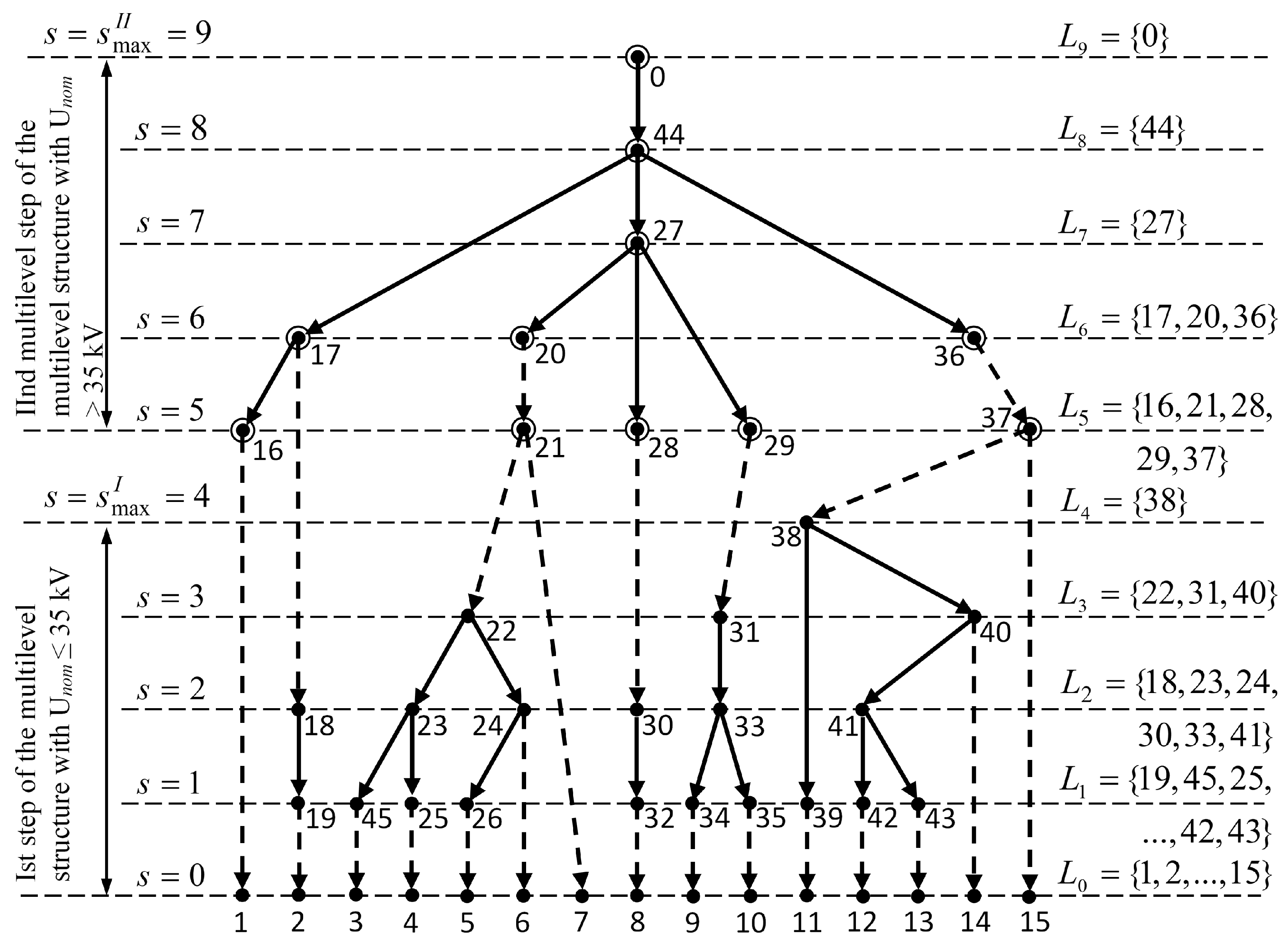
3.2. Representation of the Initial Network Graph in the Form of a Hierarchical Multilevel Structure with Two Steps of the Nominal Voltage

The example of the representation process result is presented on the Figure 3.

Step 0. 

Calculate $s=0$ and form the set of vertices of the $s=0$-th level of the hierarchy from the terminal vertices of the initial network graph, i.e., $L_0$ set;

Step 1. 

Form the initial state of the sets $L_s^H$, $L_s^L$ (where $s=0$):

$$L_0^H=L\backslash L_0,L_0^L=L_0$$

(5)

Step 2. 

Set the initial value of the step number of the nominal voltage: $a=0$;

Step 3. 

Calculate the next step number: $a=a+1$;

Step 4. 

Calculate the number of the next top level in the hierarchy: $s=s+1$;

Step 5. 

If $a=1$, then form a set $L_s$ of informationally secured vertices of the s-th hierarchy level of the multilevel structure first step with $U_{nom}\le 35$ kV:

$$L_s=\left\{i\in L_{s-1}^H\mid (\Gamma \left(i\right)\subseteq L_{s-1}^L)\wedge (U_{nom,i}\le 35\text{kV})\right\}.$$

(6)

Step 6. 

If $a=2$, then form a set $L_s$ informationally secured vertices of the s-th hierarchy level of the second step of the multilevel structure with $U_{nom}>35$ kV:

$$L_s=\left\{i\in L_{s-1}^H\mid (\Gamma \left(i\right)\subseteq L_{s-1}^L)\wedge (U_{nom,i}>35\text{kV})\right\}.$$

(7)

Step 7. 

If $L_s\ne \varnothing$, then calculate the new state of the sets $L_s^H$, $L_s^L$:

$$L_s^H=L_{s-1}^H\backslash L_s,$$

(8)

$$L_s^L=L_{s-1}^L\cup L_s,$$

(9)

where $L_s^H\cup L_s^L=L$, $\forall s\in \left\{0,1,2,\dots \right\}$.

Step 8. 

If $L_s=\varnothing$, then go to step 9, otherwise go to step 4.

Step 9. 

If $a=1$, then:

$$s=s-1,s_{max}^I=s.$$

(10)

Step 10. 

If $a=2$, then:

$$s=s-1,s_{max}^{II}=s.$$

(11)

Step 11. 

If $L_s^H\ne \varnothing$ (or $L_s^L\ne L$), then go to step 3; otherwise, go to the block for calculating power flows and losses of electricity in the network, i.e., to step 12. The results of this algorithm are:

• Set of level numbers $\left\{0,1,2,\dots ,s_{max}^I\right\}$ of the first multilevel structure level with $U_{nom}\le 35$ kV;
• Set of level numbers $\left\{s_{max}^I+1,s_{max}^I+2,\dots ,s_{max}^{II}\right\}$ of the second multilevel structure level with $U_{nom}>35$ kV;
• The set of network graph vertices for each s-th hierarchy level: $L_s$, $\forall s\in \left\{0,1,2,\dots ,s_{max}^I,s_{max}^{II}\right\}$.

3.3. Calculation of Power Flows and Losses of Electricity in Networks with Different Nominal Voltages

Step 12. 

Set loads power ${\underline{S}}_j,\forall j\in L_0$ and power source voltage $U_0$ denotes node $i=0$ voltage;

Step 13. 

Calculate $c=1$, $k=0$ and for the $k=0$ iteration take the voltage at the network nodes equal to the nominal:

$${\underline{U}}_{i\left(0\right)}=U_{nom,i},\forall i\in L\backslash \left\{0\right\}.$$

(12)

Step 14. 

Calculate the number of the next step of the iteration: $k=k+1$.

Step 15. 

Formulation of the computing process structure when calculating a network power flow with different nominal voltages:

• Formulation of the calculation structure for the $k=1$ iteration:

  $$\begin{array}{c}\hspace{0.17em}\hspace{0.17em}\text{if}k=1,\text{then}\hfill \\ \{x_{min1}=0,x_{max1}=s_{max}^{II},\hfill \\ \hspace{0.17em}\hspace{0.17em}{x}_{min2}=s_{max}^I,x_{max2}=s_{max}^{II}\};\hfill \end{array}$$

  (13)
• Formulation of the calculation structure for the $k>1$ and the stop condition:

  $$\begin{array}{c}\hspace{0.17em}\hspace{0.17em}\text{if}k>1,\text{then}\hfill \\ \{\text{if}\left(\left|U_{j(k-1)}-U_{j(k-2)}\right|>ϵ,\forall j\in \bigcup _{i\in L_{(s_{max}^I+1)}}{\Gamma }_i\right),\text{then}\hfill \\ \{x_{min1}=s_{max}^I,x_{max1}=s_{max}^{II},\hfill \\ \hspace{0.17em}\hspace{0.17em}{x}_{min2}=s_{max}^I,x_{max2}=s_{max}^{II},\hfill \\ \hspace{0.17em}\hspace{0.17em}\Delta {\underline{S}}^{\left(p\right)}=0,\forall p\in \left\{1,2,\dots ,6\right\}\},\text{otherwise}\hfill \\ \{c=0,x_{min2}=0,x_{max2}=s_{max}^I\}\},\hfill \end{array}$$

  (14)

  where $x_{min1}$, $x_{max1}$ denote, respectively, the lower and upper limits of changing the number of the hierarchy level s at the first stage (from bottom to top); $x_{min2}$, $x_{max2}$ denote respectively, the lower and upper limits of the change in s at the second stage (from top to bottom); $c\in \left\{0,1\right\}$ denotes the Boolean value to disable ($c=0$) and enable ($c=1$) of the computational module “from bottom to top” at the last cycle of the iteration k; $\Delta {\underline{S}}^{\left(p\right)}=0,\forall p\in \left\{1,2,\dots ,6\right\}$ denotes total power losses for different types of sections (see Figure 2 and Table 1).

First stage. 

Calculation of flow distribution (module algorithm “from bottom to top”).

Step 16. 

If $c=1$, then go to step 17; otherwise, go to step 21.

Step 17. 

Calculate the initial value of the hierarchy level number: $s=x_{min1}$.

Step 18. 

Calculate the number of the next top level in the hierarchy: $s=s+1$.

Step 19. 

For each Section $(i,j)\in {\Gamma }_i$ and each $i\in L_s$, calculate:

• Power losses $\Delta {\underline{S}}_{ij\left(k\right)}$ in resistance ${\underline{Z}}_{ij}$ of Section $(i,j)$ to calculate the total loss of electricity in the network;
• Power flow $({\underline{S}}_{ij\left(k\right)}{)}^{sZ}$ at the beginning of the resistance ${\underline{Z}}_{ij}$ in Section $(i,j)$ for voltage ${\underline{U}}_{j\left(k\right)}$ calculation at the end of Section j in the second stage;
• Power flow ${\underline{S}}_{ij\left(k\right)}^s$ at the beginning of Section $(i,j)$ to calculate the power flow of the node i;
• Power flow ${\underline{S}}_{i\left(k\right)}$ of the node i.

The above power flows, depending on the type of sites $(i,j)$, are calculated as follows (see Figure 2 and Table 1):

• For the sections $(i,j)$ with double-winding transformers with $U_{nom,i}>35$ kV (as can be seen in Figure 2a and Table 1, line 1):

  $$\begin{array}{cc}\hfill & \text{if}\left((j\notin L_Y)\wedge \left(U_{nom,i}>35\text{kV}\right)\wedge \left(U_{nom,i}>U_{nom,j}\right)\right),\hfill \\ \hfill & \text{then}\{\left[\Delta {\underline{S}}_{ij\left(k\right)},{\underline{S}}_{ij\left(k\right)}^{sZ},{\underline{S}}_{ij\left(k\right)}^s\right]=F_S^{\left(1\right)}\left[{\underline{S}}_{j\left(k\right)},{\underline{U}}_{i(k-1)},U_{j(k-1)}\right],\hfill \\ \hfill & \Delta {\underline{S}}^{\left(1\right)}=\Delta {\underline{S}}^{\left(1\right)}+\Delta {\underline{S}}_{ij\left(k\right)}\};\hfill \end{array}$$

  (15)
• For the sections $(i,j)$ with overhead power lines with $U_{nom,i}>35$ kV (as can be seen in Figure 2b and Table 1, line 2):

  $$\begin{array}{cc}\hfill & \text{if}\left((j\notin L_Y)\wedge (U_{nom,i}>35\text{kV})\wedge (U_{nom,i}=U_{nom,j})\right),\hfill \\ \hfill & \text{then}\{\left[\Delta {\underline{S}}_{ij\left(k\right)},{\underline{S}}_{ij\left(k\right)}^{sZ},{\underline{S}}_{ij\left(k\right)}^s\right]=F_S^{\left(2\right)}\left[{\underline{S}}_{j\left(k\right)},U_{i(k-1)},U_{j(k-1)}\right],\hfill \\ \hfill & \Delta {\underline{S}}^{\left(2\right)}=\Delta {\underline{S}}^{\left(2\right)}+\Delta {\underline{S}}_{ij\left(k\right)}\};\hfill \end{array}$$

  (16)
• For the sections $(i,j)$ with double-winding transformers with $U_{nom,i}\le 35$ kV (as can be seen in Figure 2c and Table 1, line 3):

  $$\begin{array}{cc}\hfill & \text{if}\left((j\notin L_Y)\wedge (U_{nom,i}\le 35\text{kV})\wedge (U_{nom,i}>U_{nom,j})\right),\hfill \\ \hfill & \text{then}\{\left[\Delta {\underline{S}}_{ij\left(k\right)},{\underline{S}}_{ij\left(k\right)}^{sZ},{\underline{S}}_{ij\left(k\right)}^s\right]=F_S^{\left(3\right)}\left[{\underline{S}}_{j\left(k\right)},U_{j(k-1)}\right],\hfill \\ \hfill & \Delta {\underline{S}}^{\left(3\right)}=\Delta {\underline{S}}^{\left(3\right)}+\Delta {\underline{S}}_{ij\left(k\right)}\};\hfill \end{array}$$

  (17)
• For the sections $(i,j)$ with overhead power lines with $U_{nom,i}\le 35$ kV (as can be seen in Figure 2d and Table 1, line 4):

  $$\begin{array}{cc}\hfill & \text{if}\left((j\notin L_Y)\wedge (U_{nom,i}\le 35\text{kV})\wedge (U_{nom,i}=U_{nom,j})\right),\hfill \\ \hfill & \text{then}\{\left[\Delta {\underline{S}}_{ij\left(k\right)},{\underline{S}}_{ij\left(k\right)}^{sZ},{\underline{S}}_{ij\left(k\right)}^s\right]=F_S^{\left(4\right)}\left[{\underline{S}}_{j\left(k\right)},U_{j(k-1)}\right],\hfill \\ \hfill & \Delta {\underline{S}}^{\left(4\right)}=\Delta {\underline{S}}^{\left(4\right)}+\Delta {\underline{S}}_{ij\left(k\right)}\};\hfill \end{array}$$

  (18)
• For the sections $(i,j)$ with primary windings of three-winding transformers with $U_{nom,i}>35$ kV (as can be seen in Figure 2e and Table 1, line 5):

  $$\begin{array}{cc}\hfill & \text{if}\left((j\in L_Y)\wedge (U_{nom,i}>35\text{kV})\wedge (U_{nom,i}=U_{nom,j})\right),\hfill \\ \hfill & \text{then}\{\left[\Delta {\underline{S}}_{ij\left(k\right)},{\underline{S}}_{ij\left(k\right)}^{sZ},{\underline{S}}_{ij\left(k\right)}^s\right]=F_S^{\left(5\right)}\left[{\underline{S}}_{j\left(k\right)},U_{i(k-1)},U_{j(k-1)}\right],\hfill \\ \hfill & \Delta {\underline{S}}^{\left(5\right)}=\Delta {\underline{S}}^{\left(5\right)}+\Delta {\underline{S}}_{ij\left(k\right)}\};\hfill \end{array}$$

  (19)
• For the sections $(i,j)$ with secondary windings of three-winding transformers with $U_{nom,i}>35$ kV (as can be seen in Figure 2e and Table 1, line 6):

  $$\begin{array}{cc}\hfill & \text{if}\left((i\in L_Y)\wedge (U_{nom,i}>35\text{kV})\wedge (U_{nom,i}>U_{nom,j})\right),\hfill \\ \hfill & \text{then}\{\left[\Delta {\underline{S}}_{ij\left(k\right)},{\underline{S}}_{ij\left(k\right)}^{sZ},{\underline{S}}_{ij\left(k\right)}^s\right]=F_S^{\left(3\right)}\left[{\underline{S}}_{j\left(k\right)},U_{j(k-1)}\right],\hfill \\ \hfill & \Delta {\underline{S}}^{\left(6\right)}=\Delta {\underline{S}}^{\left(6\right)}+\Delta {\underline{S}}_{ij\left(k\right)}\}.\hfill \end{array}$$

  (20)

Using the obtained power flows ${\underline{S}}_{ij\left(k\right)}^s$,$\forall (i,j)\in {\Gamma }_i$,$\forall i\in L_s$, calculate the power flows for each node $i\in L_s$:

$${\underline{S}}_{i\left(k\right)}=\sum _{j\in {\Gamma }_i}{\underline{S}}_{ij\left(k\right)}^s,\forall i\in L_s.$$

(21)

Step 20. 

If $s<x_{max1}$, then go to step 18; otherwise, go to step 21.

Second stage. 

Calculation of voltages in network nodes (module algorithm “from top to bottom”).

Step 21. 

Calculate the initial hierarchy level number $s=x_{max2}$.

Step 22. 

Calculate voltage ${\underline{U}}_{j\left(k\right)}$ and its module $U_{j\left(k\right)}$ for the ending node j of every Section $(i,j)\in {\Gamma }_i$ to calculate the flow distribution at the first stage of the next $k+1$ iteration, and phase ${\delta }_{j\left(k\right)}$:

• For the sections $(i,j)$ with double-winding transformers or for the sections $(i,j)$ with secondary windings of three-winding transformers:

  $$\begin{array}{cc}\hfill & \text{if}\left(U_{nom,i}>U_{nom,j}\right),\hfill \\ \hfill & \text{then}\left\{\left[{\underline{U}}_{j\left(k\right)},U_{j\left(k\right)},{\delta }_{j\left(k\right)}\right]=F_U^{\left(1\right)}\left[{\underline{U}}_{i\left(k\right)},U_{i\left(k\right)},{\underline{S}}_{ij\left(k\right)}^{sZ}\right]\right\};\hfill \end{array}$$

  (22)
• For the sections $(i,j)$ with overhead power lines or for the sections $(i,j)$ with primary windings of three-winding transformers:

  $$\begin{array}{cc}\hfill & \text{if}\left(U_{nom,i}=U_{nom,j}\right),\hfill \\ \hfill & \text{then}\left\{\left[{\underline{U}}_{j\left(k\right)},U_{j\left(k\right)},{\delta }_{j\left(k\right)}\right]=F_U^{\left(2\right)}\left[{\underline{U}}_{i\left(k\right)},U_{i\left(k\right)},{\underline{S}}_{ij\left(k\right)}^{sZ}\right]\right\}.\hfill \end{array}$$

  (23)

Step 23. 

Calculate the number of the next low level in the hierarchy: $s=s-1$.

Step 24. 

If $s>0$, then go to step 22; otherwise, go to step 25.

Step 25. 

If $c=1$, then go to step 14; otherwise, go to step 26.

Step 26. 

Calculate the total losses of power and electricity in the network:

$$\Delta {\underline{S}}_C=\sum _{p=1}^6\Delta {\underline{S}}^{\left(p\right)}=\Delta P_C+j\Delta Q_C;$$

(24)

$$\Delta W_C=\Delta t·\Delta P_C,$$

(25)

where $\Delta t$ denotes the time interval during which the voltage of the source and the power of the loads are constant, meaning that:

$${\underline{U}}_0=const,{\underline{S}}_j=const,\forall j\in L_0.$$

(26)

The stated approach is focused on applications of radial distribution networks in models. Most usage practices include the calculation and analysis of power supply networks at the design stage and during operation—in addition to modernization. The model’s strong points embrace a detailed presentation of network elements following physical processes characteristics; system analysis and accounting for interaction impact; simplicity algorithmization and the automation of existing power supply systems. Disadvantages are associated with the difficulty of applying to complex-closed electrical networks, which reduces the method versatility.

4. Conclusions

In this work, a structured hierarchical multilevel approach to the calculation of power flows and losses of electricity in radial electrical networks with different nominal voltages at given loads and voltage of the power source was developed. This approach is based on the representation of the initial network graph in the form of a hierarchical multilevel structure, divided into two stages with nominal voltages $U_{nom}\le 35$ kV and $U_{nom}>35$ kV, and on the use of the traditional (manual) engineering two-stage method, where the calculation is performed in a certain sequence, moving along the network structure from bottom to top (stage 1) and from top to bottom (stage 2).

Since the network of the class under consideration consists of different types of sections (power lines with $U_{nom}\le 35$ kV and $U_{nom}>35$ kV, double-winding transformers with $U_{nom}\le 35$ kV and $U_{nom}>35$ kV, primary and secondary windings of three-winding transformers (autotransformers)), then for the organization of the computational process, conditions and predicate functions are established for the choice of equivalent circuits and the corresponding calculation formulas for each type of sections. This also provides for the separation of the computational process for two stages of a hierarchical multilevel structure, for the first stage, a two-stage method with one pass from bottom to top and from top to bottom, and for the second stage, a two-stage iterative method.

The algorithm development as well as the solution of specialized problems highlighted in related works [2,6], involves the further investigation and implementation of software with increased productivity in industrial processes. At the same time, based on this approach, the authors are conducting research to increase the universality of the algorithm’s application. Promising results suggest that one could obtain an algorithm based on this one with the possibility of using it in complex-closed networks.

References

1. Chen, B.; Xiang, K.; Yang, L.; Su, Q.; Huang, D.; Huang, T. Theoretical Line Loss Calculation of Distribution Network Based on the Integrated Electricity and Line Loss Management System. In Proceedings of the 2018 China International Conference on Electricity Distribution (CICED), Tianjin, China, 17–19 September 2018; pp. 2531–2535. [Google Scholar] [CrossRef]
2. Asanov, M.; Asanova, S.; Safaraliev, M.; Lyukhanov, E.; Tavlintsev, A.; Shelyug, S. Elementwise power losses calculation in complex distribution power networks represented by hierarchical-multilevel topology structure. Prz. Elektrotechniczny 2021, 11, 106–110. [Google Scholar] [CrossRef]
3. Ghosh, S.; Sherpa, K.S. An Efficient Method for Load-Flow Solution of Radial Distribution Networks. Int. J. Electr. Comput. Eng. 2008, 2, 2094–2101. [Google Scholar]
4. Aravindhababu, P.; Ganapathy, S.; Nayar, K. A novel technique for the analysis of radial distribution systems. Int. J. Electr. Power Energy Syst. 2001, 23, 167–171. [Google Scholar] [CrossRef]
5. Wang, J.; Guo, Z.; Yu, J. Practical calculation method of theoretical line loss in 10 kv power distribution network based on Dscada. In Proceedings of the 2008 China International Conference on Electricity Distribution, Guangzhou, China, 10–13 December 2008; pp. 1–6. [Google Scholar] [CrossRef]
6. Asanova, S.; Safaraliev, M.; Askarbek, N.; Semenenko, S.; Aktaev, E.; Kovaleva, A.; Lyukhanov, E.; Staymova, E. Calculation of power losses at given loads and source voltage in radial networks of 35 kV and above by hierarchical-multilevel structured topology representation. Prz. Elektrotechniczny 2021, 1, 15–20. [Google Scholar] [CrossRef]
7. Moreira Rodrigues, C.E.; de Lima Tostes, M.E.; Holanda Bezerra, U.; Mota Soares, T.; de Matos, E.O.; Serra Soares Filho, L.; dos Santos Silva, E.C.; Ferreira Rendeiro, M.; da Silva Moura, C.J. Technical Loss Calculation in Distribution Grids Using Equivalent Minimum Order Networks and an Iterative Power Factor Correction Procedure. Energies 2021, 14, 646. [Google Scholar] [CrossRef]
8. Queiroz, L.M.O.; Roselli, M.A.; Cavellucci, C.; Lyra, C. Energy Losses Estimation in Power Distribution Systems. IEEE Trans. Power Syst. 2012, 27, 1879–1887. [Google Scholar] [CrossRef]
9. Pavičić, I.; Ivanković, I.; Župan, A.; Rubeša, R.; Rekić, M. Advanced Prediction of Technical Losses on Transmission Lines in Real Time. In Proceedings of the 2019 2nd International Colloquium on Smart Grid Metrology (SMAGRIMET), Split, Croatia, 9–12 April 2019; pp. 1–7. [Google Scholar] [CrossRef]
10. Vempati, N.; Shoults, R.R.; Chen, M.S.; Schwobel, L. Simplified Feeder Modeling for Loadflow Calculations. IEEE Trans. Power Syst. 1987, 2, 168–174. [Google Scholar] [CrossRef]
11. Pansini, A. Power Transmission and Distribution, 2nd ed.; River Publishers: New York, NY, USA, 2005; p. 414. [Google Scholar]
12. Mahmoud, K.; Yorino, N.; Ahmed, A. Optimal Distributed Generation Allocation in Distribution Systems for Loss Minimization. IEEE Trans. Power Syst. 2016, 31, 960–969. [Google Scholar] [CrossRef]
13. Hung, D.Q.; Mithulananthan, N.; Bansal, R.C. Analytical Expressions for DG Allocation in Primary Distribution Networks. IEEE Trans. Energy Convers. 2010, 25, 814–820. [Google Scholar] [CrossRef]
14. Acharya, N.; Mahat, P.; Mithulananthan, N. An analytical approach for DG allocation in primary distribution network. Int. J. Electr. Power Energy Syst. 2006, 28, 669–678. [Google Scholar] [CrossRef]
15. Kansal, S.; Kumar, V.; Tyagi, B. Optimal placement of different type of DG sources in distribution networks. Int. J. Electr. Power Energy Syst. 2013, 53, 752–760. [Google Scholar] [CrossRef]
16. Murthy, V.; Kumar, A. Comparison of optimal DG allocation methods in radial distribution systems based on sensitivity approaches. Int. J. Electr. Power Energy Syst. 2013, 53, 450–467. [Google Scholar] [CrossRef]
17. Kalambe, S.; Agnihotri, G. Loss minimization techniques used in distribution network: Bibliographical survey. Renew. Sustain. Energy Rev. 2014, 29, 184–200. [Google Scholar] [CrossRef]
18. Jain, N.; Singh, S.N.; Srivastava, S.C. A Generalized Approach for DG Planning and Viability Analysis Under Market Scenario. IEEE Trans. Ind. Electron. 2013, 60, 5075–5085. [Google Scholar] [CrossRef]
19. Vatani, M.; Alkaran, D.S.; Sanjari, M.J.; Gharehpetian, G.B. Multiple distributed generation units allocation in distribution network for loss reduction based on a combination of analytical and genetic algorithm methods. IET Gener. Transm. Distrib. 2016, 10, 66–72. [Google Scholar] [CrossRef]
20. Begovic, M. Electrical Transmission Systems and Smart Grids, 1st ed.; Springer: New York, NY, USA, 2013; pp. VI, 326. [Google Scholar]
21. Shahnia, F.; Arefi, A.; Ledwich, G. Electric Distribution Network Planning, 1st ed.; Springer: Singapore, 2013; pp. XVI, 381. [Google Scholar]
22. Asanova, S.M.; Ahyoev, J.S.; Askarbek, N.; Suerkulov, S.M.; Asanova, D.U.; Safaraliev, M.K. Method for designing drop-of-wire recognition systems on sections of undistorted two-wire power transmission lines. In IOP Conference Series: Materials Science and Engineering; IOP Publishing: Bristol, UK, 2020; Volume 966, p. 012114. [Google Scholar] [CrossRef]
Figure 1. Graph of a radial electrical network with different rated voltages.
Energies 15 00765 g001
Figure 2. Equivalent circuits of network elements with different nominal voltages.
Energies 15 00765 g002
Figure 3. Hierarchical-multilevel structure of the initial network graph ( L , Γ ) with two nominal voltage subnetworks.
Energies 15 00765 g003