Reactive Transport: A Review of Basic Concepts with Emphasis on Biochemical Processes

Abstract

Reactive transport (RT) couples bio-geo-chemical reactions and transport. RT is important to understand numerous scientific questions and solve some engineering problems. RT is highly multidisciplinary, which hinders the development of a body of knowledge shared by RT modelers and developers. The goal of this paper is to review the basic conceptual issues shared by all RT problems, so as to facilitate advancement along the current frontier: biochemical reactions. To this end, we review the basic equations to indicate that chemical systems are controlled by the set of equilibrium reactions, which are easy to model, but whose rate is controlled by mixing. Since mixing is not properly represented by the standard advection-dispersion equation (ADE), we conclude that this equation is poor for RT. This leads us to review alternative transport formulations, and the methods to solve RT problems using both the ADE and alternative equations. Since equilibrium is easy, difficulties arise for kinetic reactions, which is especially true for biochemistry, where numerous challenges are open (how to represent microbial communities, impact of genomics, effect of biofilms on flow and transport, etc.). We conclude with the basic eleven conceptual issues that we consider fundamental for any conceptually sound RT effort.

1. Introduction

The term reactive transport (RT) describes the simultaneous occurrence of (bio- and/or geo-) chemical reactions and transport of biochemical species (Figure 1). RT is important to understand numerous Earth Sciences problems, ranging from engineering applications (geologic carbon storage, enhanced geothermal systems, or groundwater remediation, etc.), as well as geological studies (such as sediment diagenesis, seismic activities, hydrothermal ore deposition, etc.) to watershed or global issues [1]. We are specifically motivated by contaminant removal during artificial recharge [2,3], which is driven by biochemical reactions.

The importance we attribute to RT contrasts with its impact in the literature. It is frequent to start a review with a bibliometric analysis to highlight the importance of the field. We searched for “reactive transport” in the Science Citation Index Expanded (SCIE) bibliographic database. Results are quite sobering (Figure 2): only 4880 papers, mostly coming from Environmental and Earth Sciences (very few from Health Sciences). Worse, the most cited papers are not “strictly” RT papers. The first and third most cited papers are quite general papers in Soil Science [4] and Seawater Intrusion [5]. The third one refers to non-Fickian transport [6]. The fourth one describes a specific surface reaction [7]. The four are relevant but not really RT papers by themselves. It is clear that this kind of search does not portray an accurate picture of the field. In fact, the list does not include the early works of Rubin and James [8], Grove and Wood [9] or Lichtner [10], who set the basis for the current paradigm of RT. However, the list is more complete for recent years, which may reflect that the reactive transport term only became common in the 1990s. Since then, the growth has been steady, albeit only linear, which is modest compared to the standard exponential growth of sister fields (e.g., Cao et al. [11]).

Figure 1. Reactive transport (RT) describes the transport of solutes (displacement by advection, spreading by dispersion, and dilution by mixing) and the reactions (red arrow) among solutes and with immobile phases. The mathematical nature of RT depends on the type of reactions and species involved [12].

Figure 1. Reactive transport (RT) describes the transport of solutes (displacement by advection, spreading by dispersion, and dilution by mixing) and the reactions (red arrow) among solutes and with immobile phases. The mathematical nature of RT depends on the type of reactions and species involved [12].

Figure 2. The number of papers identified as dealing with RT in the SCIE has increased linearly since 1993.

Figure 2. The number of papers identified as dealing with RT in the SCIE has increased linearly since 1993.

A second issue that emerges from the search is the large number of review papers (174, or 3.6% of the RT papers identified in the SCIE). We attribute the large number of reviews not so much to the difficulty of RT as to its diversity. RT reviews are driven by the nature of the chemical system, by the type of medium, by the types of reactions, or by the solution approach, etc. Several reviews emphasize geochemical issues [13]. Some are centered on problems related to ${\mathrm{CO}}_2$ storage [14,15], which generates acidity, so it is somewhat related to acid mine drainage [16], more formally revised by Amos et al. [17]. Nuclear waste disposal has motivated reviews on uranium mobility [18], validity of existing models [19], cement–clay interaction [20] or oxygen transport at depth, which motivated the thorough review of MacQuarrie and Mayer [21] on RT in fractured rock. Global issues motivate the reviews of Dignac et al. [22] and Li et al. [23]. Arndt at al. [24] and Regnier et al. [25] concentrate on degradation of organic carbon in marine sediments. Wetlands are reviewed by Langergraber [26]. Energy related subsurface problems are starting to consider RT [27,28,29,30].

Numerous recent works address the multiscale nature of the RT, especially in evolving porous media [31,32,33,34,35], pore scale and pore network models [36,37]. Finally, many papers review and/or compare methods and codes [38,39,40].

We feel that the modest publication record and parallel growth on reviews may reflect a limited interest. That is, scientists are interested, but funding agencies not so much (you may reach similar conclusions at a far lower effort). Beyond difficulty (either in understanding and/or publishing), multidisciplinarity is another difficulty with RT, which involves specialists in transport and in reactions. The former typically includes quantitatively oriented hydrologists, engineers and physicists. The latter might sound as though it is referring to chemists, but it refers to a broad and heterogeneous group which includes geochemists (originally geologists), chemists, molecular biologists and many others. They are all needed but their languages are so different that working together is not easy. Multidisciplinarity is often hallowed, but interdisciplinary work requires time and a determined effort in developing shared language and understanding. Worse, in practice it is penalized by evaluation panels. Methods cannot be shared by the various specialists, but concepts can.

The goal of this paper is to frame and review basic RT conceptual issues, which we highlight, with special emphasis on the fast-growing biochemical field, both because of our own interest and because we feel the need for shared concepts is acute. Most of the conceptual issues are widely accepted but might go unnoticed to newcomers into the RT field. Some of them are sufficiently old to be treated in textbooks (e.g., geochemical zonation), but some are not (e.g., importance and impacts of mixing, or geochemical localization). We will not enter into the fascinating world of parameter estimation [41,42,43] nor on the numerous applications of RT, which are discussed in the field-specific reviews mentioned above, except for illustrating conceptual issues.

We start with the basic equations for transport (Advection Dispersion Equation, or ADE) and reactions (Section 2 may be a bit too mathematical for some, but we request the reader to try and concentrate on the concepts). These equations allow us to frame simple reactive transport paradigms (Section 3) that illustrate what we consider the main conceptual issues of RT. In turn, the importance of properly representing mixing motivates Section 4, where we analyze transport equations other than the RT. Biochemical concepts are reviewed in Section 5 and solution methods in Section 6.

2. Basic Equations

Conceptual Issue No. 1 is that RT is multidisciplinary and requires interdisciplinarity. It is clear that many important questions can only be overcome by overlapping knowledge from different science branches, which requires working together and understanding each other. Thus, we start by reviewing the basic equations and concepts for transport and reactions.

2.1. Transport

Transport requires knowing the time and space variability of fluid fluxes. These are obtained from the flow equation, usually solved prior to transport, which requires establishing conservation of fluid mass and momentum. Fluid mass conservation is expressed as (see notation table at the end of the paper):

$$\frac{\partial \rho \varphi }{\partial t}=-\mathrm{\nabla }\cdot \left(\rho q\right)+{\rho }_e{f}_w$$

(1)

where $\rho \left[M_w/L_w^3\right]$ is fluid density, $\varphi$[–] is volumetric water content (porosity in saturated media, and $\varphi =1$ in pore scale simulations or when flow is solved in a fluid continuum, e.g., ocean), $q \left[L_w^3/L_m^2/T\right]$ is the volumetric fluid flux (usually called Darcy velocity in porous media, but only a true fluid velocity when $\varphi =1$), $f_w \left[L_w^3/L_m^3/T\right]$ represents volumetric fluid sink and sources of inflowing external water with density ${\rho }_e \left[M_w/L_w^3\right]$, which is equal to the resident fluid density $\rho$ for sinks (i.e., when $f_w<0$). Note that, given the possibility of confusion, we find it useful to express units using not only the “first name” (e.g., L, T or M), but also the “last name” (i.e., subindex $w$ for water, actually fluid in general, or $m$ for medium).

Mass conservation needs to be coupled to momentum conservation, given by the Navier–Stokes equation. The latter can be simplified to Stokes equation when flow is laminar, which is the usual assumption in pore scale analyses (e.g., [36]), or further simplified to Darcy’s Law when the laminar flow is slow (i.e., inertial effects can be neglected) and the porous medium is treated as a continuum [44].

Transport is usually solved with the advection-dispersion equation (ADE, sometimes ADRE, with the R standing for reaction), a partial differential equation (PDE) that expresses the mass balance of each aqueous species when transport is driven by advection and dispersion. Beyond the mathematical complexities, Figure 1 implies that concentration changes due to the following processes:

•  Advection, that is, the displacement of solutes dragged by fluid flow. Note that, unless flow is solved at the pore scale, advection is represented with a mean fluid flux (mean over a volume that depends on the level of detail with which flow has been solved).
•  Dispersion includes two processes: molecular diffusion (i.e., Brownian motion causes a solute mass flux away from high concentration regions, given by Fick’s Law) and velocity fluctuations with respect to the mean fluid flux, which causes the solute to spread (also written by a Fick’s-like Law). We will revisit this term in Section 4.
•  External sources, solute mass that leaves/enters the medium with fluid sink and sources, $f_w$.
•  Chemical reactions, which may cause concentration to increase (e.g., mineral dissolution) or decrease (e.g., precipitation).

The ADE results from explicitly expressing mass conservation (per unit volume of medium and unit time) for the above four processes, which yields:

$$\frac{\partial \rho \varphi c_{a,i}}{\partial t}=-\mathrm{\nabla }\rho q{c}_{a,i}+\mathrm{\nabla }\cdot \left(\rho D·\mathrm{\nabla }{c}_{a,i}\right)+{\rho }_e{c}_{ex,i}{f}_w+R_i i=1,\cdots , N_a$$

(2)

$$\frac{\partial \rho \varphi c_{s,i}}{\partial t}=R_{s,i} i=1, N_s$$

(3)

where $c_i\left[M_{sol}/M_w\right]$ is the concentration of species $i$ (aqueous or immobile depending on the subscript, $a$ or $s$, respectively), $D$[L²/T] is the hydrodynamic dispersion tensor ($D_{pq}=\varphi D_m{\delta }_{pq}+{\alpha }_{T}q{\delta }_{pq}+\left({\alpha }_L-{\alpha }_T\right)q_p{q}_q/q$, where $q$ is the modulus of flux, $q=\left|q\right|$, and $q_p$ its $p$-th component; $D_{mp}=\varphi D_m$ is the effective molecular diffusion, $c_{ex.i}$ is the concentration of species $i$ in fluid sources (again, $c_{ex,i}=c_i$ when $f_w<0$) and $R_i \left[M_{sol}/L_m^3/T\right]$ includes the contributions of chemical reactions to the mass balance of species $i$, expressed per unit volume of porous medium. This equation is somewhat cumbersome (in part because of the units we have chosen). In fact, it can be written in various forms depending on the context. For example, it is frequent to write $D$ in terms of velocities instead of fluxes for historical reasons, but this is inconvenient in porous media, where velocity is poorly defined (it depends on the model, whereas water flux, given by Darcy’s Law, is a robust concept). In addition, we have written concentration as mass fraction (e.g., ppm) to ensure that dispersion does not cause advection and that adding Equation (2) for all aqueous species yields the fluid mass balance (Equation (1), e.g., [45]). However, reactions usually express the solute mass $\left[M_{sol}\right]$ in moles, so that $c_i$ can express moles of species $i$ per unit mass of solution (still a mass fraction, for practical purposes). When fluid density is taken as constant then it is valid to write transport in terms of $\rho c_i$ (molarity). However, chemical databases usually require working with molality (moles solute per kg of ${\mathrm{H}}_2\mathrm{O}$, or $m_i=c_i/{\omega }_w$, where ${\omega }_w$ is the mass fraction of ${\mathrm{H}}_2\mathrm{O}$).

The conservative form of the ADE (Equation (2)) is robust, but lacks an explicit representation of velocity, which is needed for Lagrangian methods. We can deduce a form in which velocity is explicit, by subtracting Equation (1), multiplied by $c_i$, from Equation (2), and dividing by $\rho$, which yields:

$$\varphi \frac{\partial c_{a,i}}{\partial t}=\mathrm{\nabla }\cdot \left(D·\mathit{\nabla }{c}_{a,i}\right)-q\mathit{\nabla }{c}_{a,i}+f_w\left(c_{ex,i}-c_{a,i}\right)+\frac{R_i}{\rho } i=1, \cdots , N_a$$

(4)

This advective form is conceptually rough because (1) it represents the “flow-equation[removed” [46] balance, but divided by density, and (2) the units of the mass balance are somewhat tricky $\left[M_{sol}{L}_w^3{L}_m^{-3}{M}_w^{-1}{T}^{-1}\right]$, which is why the most frequent option is to assume water incompressible and work with molarities (i.e., moles per unit volume of fluid). A somewhat easier to understand form results from dividing Equation (4) by $\varphi$, while neglecting its spatial variations for the dispersive term, which yields:

$$\frac{\partial c_{a,i}}{\partial t}=\mathrm{\nabla }\cdot \left(D_v·\mathrm{\nabla }{c}_{a,i}\right)-v\mathrm{\nabla }{c}_{a,i}+f_v\left(c_{ex,i}-c_{a,i}\right)+R_{w,i} i=1, \cdots , N_a$$

(5)

where $R_{w,i}=R_i/\varphi \rho$ is the contribution of reactions, but expressed per unit mass of fluid, $D_v$ is similar to $D$, but expressed in terms of velocity instead of fluid fluxes, and $v=q/\varphi$ is the mean water velocity. This form is preferred by many because it is identical to the transport equation used in the much broader community of fluid continuum transport, so that it facilitates recycling of codes developed in sister sciences. It is also the form preferred by the pore scale simulation community. Furthermore, it leads naturally to Lagrangian formulations of transport (e.g., Random Walk methods):

$$\frac{D{c}_{a,i}}{Dt}=\mathrm{\nabla }\cdot \left(D_v·\mathrm{\nabla }{c}_{a,i}\right)+f_v\left(c_{ex,i}-c_{a,i}\right)+R_{w,i} i=1,\cdots ,N_{as}$$

(6)

where $D{c}_i/Dt=\partial c_i/\partial t+v\mathrm{\nabla }{c}_i$ is the material derivative (i.e., the rate of concentration change in a flowing water parcel). It is important to point that all these advective forms of the ADE (Equations (4)–(6)) are equivalent to Equation (2). We have spelled them out to illustrate that the ADE can be found in numerous forms. In practice, however, advective forms require being extremely careful in the application of numerical methods. For example, very few authors use the reverse time weighting [47] for transient flow cases, which may lead to severe mass balance errors. Still, for simplicity, we write:

$$\varphi \frac{\partial c_i}{\partial t}=L\left(c_i\right)+R_i i=1,\cdots , N_s$$

(7)

where $L\left(c_{a,i}\right)=\mathrm{\nabla }\cdot \left(D·\mathrm{\nabla }{c}_{a,i}\right)-q\mathrm{\nabla }{c}_{a,i}+f_w\left(c_{ex.i}-c_{a.i}\right)$, if species $i$ is aqueous or $L\left(c_{s,i}\right)=0$, if it is immobile. Note that, written like this, the concentration of immobile species is expressed per unit volume of liquid, which is unusual. Normally, immobile species concentrations are expressed per unit mass of solid (or volume of porous medium). We will keep it as written for the sake of simplicity.

Some insight into the nature of this equation can be obtained by writing it in dimensionless form and from Figure 1. The figure shows that the basic behavior of the ADE is defined by the dispersion length $L_D=\sqrt{Dt}$, which characterizes the spread over which concentration tends to homogenize, and the advection length $L_A=qt/\varphi =vt$, distance traveled by conservative solutes. Figure 3 displays the time evolution of these two lengths for different values of $D$, $q$, and $\varphi$. It is clear that, for short times and distances, diffusion (or dispersion) dominates, but advection always dominates at long time (and space) scales. The characteristic time of the ADE is chosen as the one that equates these two lengths (i.e., $t_c=\varphi D/q^2$), which leads to a characteristic length $L_c=D/q$ and the dimensionless ADE:

$$\frac{\partial c_{D,i}}{\partial t_D}={\mathit{\nabla }}_D^2{c}_{D,i}-{\mathit{\nabla }}_D{c}_{D,i}+f_D\left(1-c_{D,i}\right)+R_{D,i}$$

(8)

where $t_D=t/t_c$, ${\mathrm{\nabla }}_{\mathrm{D}}\equiv \partial /\partial x_D$, $x_D=x/L_c$,$c_D=c_i/c_{ci}$ ($c_{ci}$ is a characteristic concentration that depends on the problem, often a boundary or initial concentration, here $c_c=c_{ex,i}$), $f_D=f_w{L}_c/q$ (i.e., the fraction of water flux, $q$, that enters the medium from internal sources, $f_w$, over $L_c$), and $R_{Di}=R_i{L}_c/q{c}_c$ (i.e., the fraction of advective solute flux, $q{c}_c$, produced by reactions over $L_c$). This dimensionless form is unusual. The most frequent choice is to select $L_c$ as a length of interest and then define the Peclet number as $Pe=L_{int}/L_c$, which appears in front of the advection term. This way, $Pe>1$ is the same as saying $L_{int}>L_c$. We prefer using Equation (8) because it makes apparent that the Peclet number is not an attribute of the ADE, but of the length of interest, which makes $Pe$ ambiguous because any problem may have numerous spatial lengths of interest. For example, under normal conditions the ADE will be diffusion dominated at the pore scale, but advection dominated at the field and laboratory scales. This discussion leads to Conceptual Issue No. 2: diffusion controls microscales; advection controls macroscales; the Peclet number is ambiguous.

Other dimensional forms are possible and, especially, many other transport equations can be chosen. We analyze them in Section 4.

2.2. Reactions

The term $R_i$ represents the contributions of all reactions to the mass balance of species $i$, expressed per unit volume of porous medium. This section is devoted to the evaluation of $R_i$. Stated this way, it may sound irreverent, given the complexity of the concepts behind it (reactions include all biogeochemical processes from mineral dissolution to hormones production). However, from an RT perspective, evaluating $R_i$ is all one needs.

The first step is to define the chemical system, that is, the set of species we are going to deal with and their reactions. In essence the chemical system is defined by:

$${{\displaystyle \sum }}_{i=1}^{N_{sp}}{S}_{ji}N{m}_i=0 j=1, \cdots ,N_r$$

(9)

where $N{m}_i$ is the chemical formula of the i-th species, $N_{sp}$ is the number of species,$N_r$ is the number of reactions, and $S_{ij}$ is the stoichiometric coefficient of species $i$ in reaction $j$. Then, $R_i$ is given by:

$$R_i={{\displaystyle \sum }}_{j=1}^{N_r}{S}_{ij}{r}_j i=1,\cdots , N_{sp}$$

(10)

where $r_j$ is the reaction rate (i.e., moles of reactants that evolve into products, per unit time and per unit volume of medium).

$$S·Nm=0$$

(11)

RT usually involves many reactions and species, which makes it convenient to write these equations in a matrix-vector notation for concise writing. Thus, we rewrite Equations (9) and (10) as:

$$R=S^{t}r$$

(12)

where $S$ is the $N_r\times N_{sp}$ stoichiometric matrix, whose rows contain the stoichiometric coefficients in each reaction, and $r$ a vector of size $N_r$, containing rates of all reactions, and $Nm$ a vector of size $N_{sp}$, containing the chemical formula of all species. To illustrate these concepts, let us consider a simple calcite dissolution problem, which one might define as consisting of three species $N{m}^t=\left(\mathrm{C}\mathrm{a}\mathrm{C}{\mathrm{O}}_{3\left(s\right)},\mathrm{C}{\mathrm{O}}_3^{2-}, \mathrm{C}{\mathrm{a}}^{2+}\right)$ and one reaction ($\mathrm{C}\mathrm{a}\mathrm{C}{\mathrm{O}}_{3\left(s\right)}-\mathrm{C}{\mathrm{O}}_3^{2-}-\mathrm{C}{\mathrm{a}}^{2+}=0$). Then, the stoichiometric coefficients would be $S=\left(1,-1,-1\right)$, so that $R_1=r_1$, $R_2=-r_1$, and $R_3=-r_1$. Note, however, that in most groundwater problems, this definition would be insufficient because most of the carbonate evolves to bicarbonate ($\mathrm{H}\mathrm{C}{\mathrm{O}}_3^{-}$) under neutral pH conditions, so that both $\mathrm{H}\mathrm{C}{\mathrm{O}}_3^{-}$ and ${\mathrm{H}}^{+}$ would have to be included in the set of species and a new reaction ($\mathrm{H}\mathrm{C}{\mathrm{O}}_3^{-}-\mathrm{C}{\mathrm{O}}_3^{2-}-{\mathrm{H}}^{+}=0$) in the set of reactions. Let this simple example serve to illustrate Conceptual Issue No. 3: it is important to select the appropriate set of species and reactions. While this may sound trivial, it is not. There are few absolute objective rules to define an “appropriate” chemical system. We come back to this issue, but for now, let us simply state that, in practice, it requires the active participation of a specialist (a geochemist for inorganic reactions, a biochemist for biochemical reactions, often both), a reminder of Conceptual Issue No. 1.

Mathematically oriented readers may use these definitions to view the chemical system as a vector space of dimension $N_{sp}$, and reactions as vectors of the changes in concentrations due to chemical reactions. This view is extensively discussed by Rubin [12] and Friedly and Rubin [48], who attribute it to Prigogine and Defay [49].

For the purpose of computing reaction rates, $r$, it is convenient to distinguish between kinetic (“slow” in Figure 1) and equilibrium (“fast” in Figure 1) reactions. Obviously, the concept of slow or fast is relative to transport time or to the characteristic time of other reactions. For now, let us simply state that kinetic reactions are those whose rate is solely controlled by the concentrations at the point where the reaction is occurring, that is $r_k=r_k\left(c\right)$, where we have introduced the subindex $k$ to indicate that, in general, only a subset of all reactions are kinetic.$r_k\left(c\right)$ are empirical functions. Lasaga [50] covers them extensively for inorganic reactions. Biochemical reactions are reviewed in Section 5. It should be noted the apparent simplicity of this expression hides the complexity of most Earth processes, including life, of course.

Equilibrium reactions are governed by the mass action law (MAL), which states that:

$$S_{\mathit{e}}\mathit{log}a=\mathit{log}{{\rm K}}_{\mathit{e}}$$

(13)

where $S_{\mathit{e}}$ consists of the $N_{\mathit{e}}$ rows of $S$ corresponding to the $N_{\mathit{e}}$ equilibrium reactions, ${{\rm K}}_{\mathit{e}}$ is the vector of their equilibrium constants and $a$ is the vector of their activities. Activity is a dimensionless quantity, related to the chemical potential of the species in solution, that quantifies its “effective” concentration (i.e., its availability to react). The activity of aqueous species should be equal to the molar fraction of the species for ideal, low salinity, solutions. Unfortunately, standard chemical databases have been introduced for molalities, so that, ideally, the activity is equal to the molality. As salinity increases, the “effective” concentration decreases, so that the activity becomes $a_i={\gamma }_i{m}_i$, where ${\gamma }_i$ is its “activity coefficient”. For moderate salinities, the molality is very close to the molarity (i.e., $a_i\approx {\gamma }_i{c}_i$). In general, however, one would need to write $a_i={\gamma }_i{c}_i/{\omega }_w$. MAL also applies for sorption to solid surfaces, where activity is expressed in mol per unit mass of solid. As we express concentrations of solid species in mol per unit mass of water (Section 2.1), the activity of adsorbed species becomes $a_{s,i}=c_{si}\rho \varphi /\left({\rho }_s{\theta }_s\right)$, where ${\rho }_s$ and ${\theta }_s$ are the density and volume fraction of the solid. For cation exchange the activity is an equivalent fraction, that is, $a_i=z_i{c}_i\rho \varphi /\left({\rho }_s{\theta }_{s}CEC\right)$, where $z_i$ is the charge of the solute and $CEC$ is the Cation Exchange Capacity expressed in equivalents per unit of mass of solid. Moreover, in some models the electrical charge of the solid is assumed to be different from that of the liquid and an electrical double layer is assumed consisting of an electrical potential that decreases rapidly away from the charged solid surface. The equilibrium constant in the MAL (Equation (13)) is corrected for the free energy associated with the electrical potential [40]. As we see in Section 3.1, model representation of sorption can range from very simple to very complex (Appelo and Postma, [51], Chapter 6). For minerals, one has to understand that the solid comprises various mineral phases. Generally, it is assumed that they are pure phases, and their activity is equal to 1.0. It is important to realize that the set of present minerals (or mineral zone), and hence the MAL, may change in space and time. The activity of gases is called fugacity, but is usually expressed in terms of pressure (in bars), so that under ideal conditions, the fugacity of a gas is equal to its partial pressure. For high pressures and temperatures, the behavior of gases is not ideal, and their partial pressure needs to be multiplied by a fugacity coefficient, analogous in concept to the activity coefficient. Note that numerous species (pure minerals, constant pressure gases, ideal ${\mathrm{H}}_2\mathrm{O}$) display constant activity. Therefore, from the chemical point of view, they are not unknowns. The number of unknowns in Equation (13) is $N_{sp}-N_c$, where $N_c$ is the number of constant activity species, a feature we will profit from later.

The equilibrium constant, K, is a characteristic of every chemical reaction that depends (a little) on pressure and (possibly a lot) on temperature. In practice, it is obtained by minimizing the Gibbs free energy of the solution or from chemical databases. The selection of the database is a topic in itself. The most widely used databases for geochemical modeling are EQ3/EQ6 [52] and PHREEQE [53]. Specific databases are often available for specific purposes. For example, [54] review data for CO2 storage. There are databases in the framework of cement/clay interactions [55] and the NEA (Nuclear Energy Agency) has produced thermochemical databases intended for the radioactive waste management community [56]. Since databases contain stoichiometric coefficients, as well as data to compute activity coefficients, and they are well-tested, we recommend using them, at the very least to reduce errors during input data preparation (this can also be performed by means of a good preprocessor).

Databases are also available for kinetic rate laws, especially for dissolution of minerals [57,58]. In general, they consist of rather empirical data from laboratory experiments. Therefore, their use at the field scale is not straightforward, as rates at the field scale are known to be different from the laboratory scale [59]. Databases are also available for kinetic biochemical reactions. Their use is less frequent because reaction rates can be written in numerous forms. A good one is the NIST Chemical Kinetics Database (https://kinetics.nist.gov/kinetics (accessed on 15 November 2021)). Things get more complicated for biochemical reactions. PubChem (https://pubchem.ncbi.nlm.nih.gov) is a “popular chemical information resource” [60] (accessed on 15 November 2021). The problem is that using it requires some expertise. For example, searching for “trichloroethylene” yields 18 compounds (the “standard” 1,1,2-trichloroethene, but also 1,1,2-trichloro-2-deuterioethene, and many others that we would never call TCE) and 185 substances. However, if you search for “trichloroethene”, another synonym of TCE for us, PubChem yields 167 compounds, but only 80 substances.

The MAL describes equilibrium conditions that species must satisfy. Therefore, Equation (13) can be viewed as a set of constraints on valid values of concentrations. Or, returning to the vector space view of chemical systems, equilibrium reactions reduce the dimensionality of the concentrations space leading to Conceptual issue No. 4: equilibrium reactions reduce the size and complexity of RT problems. The issue is illustrated in Figure 4 for a simple gypsum equilibrium example. The chemical system consists of three species (gypsum, $\mathrm{C}{\mathrm{a}}^{2+}$, and $\mathrm{S}{\mathrm{O}}_4^{2-}$). The stoichiometric matrix contains only one row describing the single reaction of the system (Figure 4a). Concentrations (Figure 4b) and activities (Figure 4c) must lie on the equilibrium line. This line is straight (i.e., linear) in log activities (Equation (13)), but non-linear in concentrations because of the logs and the activity coefficients. Note that reactions (red line) occur only when the system is driven away from the equilibrium line. They are given by Equation (12). Therefore, they are orthogonal to the equilibrium line in log activities; recall that the coefficients of a (hyper) plane equation are the components of its orthogonal vector. The concentration space is convenient for mass balance, which is given by the transport equations. The activity space is convenient for chemical calculations. In this example, knowing one activity ($a_1=a_{\mathrm{C}\mathrm{a}}$, in Figure 4c) allows easy calculation of the other ($a_2=a_{\mathrm{S}{\mathrm{O}}_4}$).

The concepts of Figure 4 are general. Each equilibrium reaction reduces the dimension of the concentrations space by 1. Therefore, the number of degrees of freedom is $N_s-N_e$ and one can choose a subset of primary species as the basis of the subspace of “valid” concentrations. The remaining $N_e$ species are called secondary. Their activities can be calculated from those of primary species through the MAL. We can write the mass action laws in terms of primary and secondary species by splitting matrix $S_e$ and vector $a$ into two parts (${\mathbf{S}}_e=\left({\mathbf{S}}_{e1},{\mathbf{S}}_{e2}\right)$; $a^t=\left(a_1^t,a_2^t\right)$), where $a_1$ contains the activities of the ($N_{sp}-N_e$) primary species and $a_2$ the remaining ($N_e$), secondary species, and where ${\mathbf{S}}_{e1}$ contains the stoichiometric coefficients for the primary and ${\mathbf{S}}_{e2}$ those for the secondary species. Substituting these definitions in Equation (13) and multiplying by ${\mathbf{S}}_{e2}^{-1}$ yields:

$$\mathit{log}{a}_2={\mathbf{S}}_{e1}^{\ast }\mathit{log}{a}_1+\mathit{log}{\mathbf{K}}^{\ast }$$

(14)

where ${\mathbf{S}}_{e1}^{\ast }=-{\left({\mathbf{S}}_{e2}\right)}^{-1}{\mathbf{S}}_{e1}$ and $\mathit{log}{\mathbf{K}}^{\ast }={\left({\mathbf{S}}_{e2}\right)}^{-1}\mathit{log}\mathbf{K}$. In this way we obtain a new description of the same chemical system, which is now defined by equilibrium constants ${\mathbf{K}}^{\ast }$ instead of $\mathbf{K}$ and of stoichiometric matrix for the primary species ${\mathbf{S}}_{e1}^{\ast }$ instead of ${\mathbf{S}}_{e1}$.

RT computations are simplified by introducing components, defined here as chemical entities that are not affected by equilibrium reactions. To this end, it is convenient to define the components matrix as the $\left(N_{sp}-N_e\right)\times N_s$ kernel matrix (or null space) of ${\mathbf{S}}_e$. That is, $U{S}_e^t=0$. In vector space nomenclature, this matrix defines the orthogonal complement to the equilibrium subspace of valid concentrations. Matrix $U$ is not unique. In fact, the set of possible component matrices is in itself a vector space of dimension $N_{sp}-N_e$. Hence, there are numerous methods to obtain it. Molins et al. (2004) describe some of them [61]. In particular, they define approaches to ensure that $U$ facilitates reactive transport computations. Still, the most widely used method is based on Gauss–Jordan elimination [62], which consists of defining the component matrix as:

$$U=\left(I,S_{e1}^t{\left(S_{e2}^t\right)}^{-1}\right)$$

(15)

where $\mathrm{I}$ is the $\left(N_s-N_e\right)$ identity matrix. It is easy to check that, indeed, ${\mathbf{US}}_e^t=0$. Components are then defined as linear combinations of species:

$$u=Uc=\left(\begin{array}{cc}I& {\left(S_1^{\ast }\right)}^t\end{array}\right)\left(\begin{array}{c}{c}_1\\ c_2\end{array}\right)=c_1+{\left(S_1^{\ast }\right)}^{\mathrm{T}}{c}_2$$

(16)

The identity matrix in the front portion of the component matrix (i.e., the one coinciding with the primary species) ensures that the components are somehow associated to the primary species. This association is sometimes weak, but examining the components often provides some insight into the chemical system. Since some species are immobile, $c^t={\left(\begin{array}{cc}{c}_a& c_s\end{array}\right)}^t$, components may also contain an immobile part. This can be formalized by splitting $U=\left(\begin{array}{cc}{U}_a& U_s\end{array}\right)$, so that $u=Uc=u_a+u_s$, where $u_a=U_{a}c$, and $u_s=U_{s}c$.

We illustrate these matrices by another simple example involving calcite (Cc) and gypsum (Gyp) dissolution precipitation in equilibrium, as shown in Figure 5. The chemical system consists of two reactions ($N_r=N_e=2$) and five species ($\mathrm{C}\mathrm{c}, \mathrm{G}\mathrm{y}\mathrm{p}, \mathrm{C}{\mathrm{a}}^{2+}, \mathrm{S}{\mathrm{O}}_4^{2-},$ and $\mathrm{C}{\mathrm{O}}_3^{2-}$, i.e., $N_{sp}=5$). Therefore, the chemical state can be defined in terms of three components or three primary species (the remaining species, secondary, can be easily obtained from Equation (14)). We choose $\mathrm{C}\mathrm{c}, \mathrm{G}\mathrm{y}\mathrm{p}$, and $\mathrm{C}{\mathrm{a}}^{2+}$ to be primary species, and $\mathrm{S}{\mathrm{O}}_4^{2-}$ and $\mathrm{C}{\mathrm{O}}_3^{2-}$ to be secondary. The corresponding stoichiometric matrix, $S_e$, is shown in the left column of Figure 5. The choice of primary and secondary species is somewhat arbitrary. The only requirement is that ${\mathbf{S}}_{e2}$ must be non-singular. In this case, ${\mathbf{S}}_{e2}$, which encompasses the last two columns of $S_e$ in Figure 5 (blue square), equals the identity matrix (${\mathbf{S}}_{e1}$ is the green square). To obtain the components matrix, we first compute ${\mathbf{S}}_{e1}^{\ast }$, defined below Equation (14):

$${\mathbf{S}}_{e1}^{\ast }=-{\left({\mathbf{S}}_{e2}\right)}^{-1}{\mathbf{S}}_{e1}=-{\left(\begin{array}{cc}1& 0\\ 0& 1\end{array}\right)}^{-1}\left(\begin{array}{ccc}0& -1& 1\\ -1& 0& 1\end{array}\right)=\left(\begin{array}{ccc}0& 1& -1\\ 1& 0& -1\end{array}\right)$$

(17)

Application of Equation (15) gives the following component matrix:

$$U=\left(I|{\left(S_{e1}^{\ast }\right)}^T\right)=\left(\begin{array}{c}\begin{array}{ccc}\mathrm{C}\mathrm{c}& \mathrm{G}\mathrm{y}\mathrm{p}& \mathrm{C}{\mathrm{a}}^{2+}\end{array}\\ \begin{array}{ccc}1& 0 & 0 \\ 0& 1& 0 \\ 0& 0& 1 \end{array}\end{array}|\begin{array}{c}\begin{array}{cc} \mathrm{S}{\mathrm{O}}_4^{2-}& \mathrm{C}{\mathrm{O}}_3^{2-}\end{array}\\ \begin{array}{cc} 0& 1\\ -1& 0\\ -1& -1\end{array}\end{array}\right) \begin{array}{c}\begin{array}{c}\\ Tot carbonate\end{array}\\ Tot Sulfate\\ Cat-Ani\end{array}$$

(18)

Total concentrations of components, $u=Uc$ (Equation (16)), can be read directly from Equation (18). The first one is total carbonate in the system (it will not change due to reactions, because carbonate must be either dissolved or in calcite). The same can be said about the second component (total sulfate). These two components contain aqueous ($u_a$) and solid immobile ($u_s$) parts. The third component ($u_3=\mathrm{C}{\mathrm{a}}^{2+}-\mathrm{S}{\mathrm{O}}_4^{2-}-\mathrm{C}{\mathrm{O}}_3^{2-}$) is conservative because gypsum dissolution and/or precipitation will change $\mathrm{C}{\mathrm{a}}^{2+}$ and $\mathrm{S}{\mathrm{O}}_4^{2-}$ by the same amount (and similarly with calcite), so that their difference remains unchanged by these reactions. In short, the three components are indeed conservative.

Figure 5. Simplified chemical system for calcite (Cc) and gypsum. The full stoichiometric matrix (blue and green squares) can be simplified (red) if mineral activities are constant (a). Equilibrium imposes constraints on concentrations, which must lie on equilibrium surfaces (b) that become planes in log activities (c). Reactions (red and purple arrows, (b)) lie on constant $u$ planes (green plane, (b)).

Figure 5. Simplified chemical system for calcite (Cc) and gypsum. The full stoichiometric matrix (blue and green squares) can be simplified (red) if mineral activities are constant (a). Equilibrium imposes constraints on concentrations, which must lie on equilibrium surfaces (b) that become planes in log activities (c). Reactions (red and purple arrows, (b)) lie on constant $u$ planes (green plane, (b)).

Actually, the problem can be further simplified (conceptually and numerically). As mentioned before, constant activity species are not really unknowns during chemical calculations and it is profitable to eliminate them. This is precisely what was done by Saaltink et al. [63]. They used Equation (15), but then multiplied the components matrix by an elimination matrix, thus reducing the number of primary species. The resulting method was the first one consistent with Gibbs rule. Another possibility is to choose the constant activity species to be primary, which is what we have done in the example of Equations (17) and (18), where calcite and gypsum are both constant activity and primary species. As the MALs do not depend on the activity of constant active species, we can decouple the calculation of the concentrations of these primary species and the transport equation of their corresponding components. In practice, the number of unknowns is reduced from $N_{sp}$ to $N_{sp}-N_c$.

The use of constant activity species is discussed further in Figure 5. If $\mathrm{Cc}$ and $\mathrm{Gyp}$ are assumed constant activity (as discussed above, this is the standard assumption for pure minerals), they are not chemical unknowns, so that the stoichiometric matrix is reduced to a 2 × 3 matrix, and the components matrix becomes a 1 × 3 matrix (red square in Figure 5, and also in Figure 4). The component space is 1D, so that any species may serve as primary. In the full concentration space, the single component (${\mathrm{Ca}}^{2+}-+{\mathrm{O}}_4^{2-}--{\mathrm{O}}_3^{2-}$) is represented as a plane orthogonal to the equilibrium (and, thus, to both the calcite and gypsum equilibrium subspaces) reactions. Reactions must stay in this plane (red and purple arrows in Figure 5) because they do not change components.

Speciation calculations are needed to obtain the vector of concentrations of all variable activity species from $a_1$ or $c_1$. In the first case, Equation (14) yields directly $a_2$. Concentrations are then obtained from the activity coefficients as $c=a/\gamma$. Iterations may still be needed because $\gamma =\gamma \left(c\right)$. However, this dependence is weak. A more problematic case arises when speciation needs to be performed from components. In this case, the $N_s$ concentrations are obtained from the MAL of the $N_e$ equilibrium reactions (Equation (12)) and the $N_s-N_e$ definitions of components (Equation (16)). The solution of these equations can be difficult and may require special solutions methods [64,65,66]. A number of codes are available to perform speciation calculations, such as PHREEQC [67], CHEPROO [68] and GEMSK [69]. Still, since these calculations need to be repeated numerous times (number of nodes times number of iterations times number of time steps), it makes them ideal for artificial neural networks [70], which is possibly what the future holds for RT.

2.3. Coupled Transport and Reactions

Reactive transport is the phenomenon resulting from the interaction and coupling of solute transport, explained in Section 2.1, and chemical reactions, explained in the previous section. Thus, reactive transport equations simply represent the mass balance of chemical species subject to both transport processes and chemical reactions. This statement suggests posing the problem as solving the system of equations:

$$\varphi \frac{\partial c}{\partial t}=L\left(c\right)+S_e^t{r}_e+S_k^t{r}_k$$

(19)

$$S_e\mathit{log}a=\mathit{log}{{\rm K}}_e$$

(20)

$$r_k=r_k\left(c\right)$$

(21)

This formulation of reactive transport contains $N_{sp}+N_r$ unknowns. These are matched by the $N_{sp}$ mass balances of all species (Equation (19)), plus the $N_e$ MAL (Equation (20)), and the $N_k$ definitions of kinetic reaction rates. The latter can be eliminated by substitution of Equation (21) into (19). Still, the large number of coupled non-linear equations makes the problem intractable. Therefore, various strategies have been proposed to simplify the problem [71,72]. However, most of them are based on eliminating the equilibrium reaction rates by multiplying Equation (19) by a component matrix, which leads to:

$$\varphi \frac{\partial u}{\partial t}=L\left(u_a\right)+U{S}_k^t{r}_k$$

(22)

Care must be taken in acknowledging the phase to which species belong. Only the aqueous fraction of components,$u_a=U_a{c}_a$, is transported. In fact, the transport operator does not apply to the solid (immobile) fraction, $u_s=U_s{c}_s$.

An important issue arises here for problems where the solid phase consists of several ideal (constant activity) minerals, depending on how components have been derived. If components were derived using all reactions in the system, then the transport equations will be the same throughout the domain, which sounds advantageous. However, if components were defined after eliminating constant activity species (reduced stoichiometric and components matrices) the transport problem would be different for every mineral zone. While this sounds disadvantageous, the reality is that the problems are indeed different, as discussed by Rubin [12]. As a result, sharp concentration fronts develop at the interface between different mineral zones because water with the conditions of the upstream chemical system must adapt instantaneously to the chemical system downstream (Figure 6).

The apparent discontinuity in Figure 6 simply reflects that the set of equations in each mineral zone will be different, thus yielding different solutions. A₃ does not participate in Min. 1 and behaves conservatively, up to x = 50, where Min. 2 leads to a new equilibrium. As mentioned above, what happens is that the RT equations are different in the two mineral zones, and a sharp reaction rate (mathematically a Dirac delta) occurs at their interface. While this is known to occur in reality, it hinders numerical solutions. The transport equation does not allow discontinuities. The solution will display a sharp front with a width comparable to dispersivity (0.3 m in the example of Figure 6). In practice, this will cause convergence problems to numerical methods that do not account explicitly for chemical heterogeneity and force modelers to use large dispersion coefficients, which may cause other problems, as we discuss in Section 3.3. Ways to overcome the problem numerically are described in Section 6. This leads to Conceptual Issue No. 5: mineral zone variations lead to sharp fronts in aqueous chemistry.

Figure 6. Transport of pulse injected at x = −8 m and t = −18 d in a medium consisting of two minerals. A front occurs for A₃ at x > 50 m, where it equilibrates with Min. 2, causing its sharp precipitation and an apparent discontinuity in concentrations. The analytical solution (A_r1) [73] is displayed for the precipitation rate of Min. 1. Reaction rates maxima coincide with gradients maxima (black arrows).

Figure 6. Transport of pulse injected at x = −8 m and t = −18 d in a medium consisting of two minerals. A front occurs for A₃ at x > 50 m, where it equilibrates with Min. 2, causing its sharp precipitation and an apparent discontinuity in concentrations. The analytical solution (A_r1) [73] is displayed for the precipitation rate of Min. 1. Reaction rates maxima coincide with gradients maxima (black arrows).

3. Basic Reactive Transport Paradigms

In the previous section, we analyzed the ADE for transport, the formulation of general chemical reactions, and how to couple them to write an RT model. We now discuss how the coupling leads to vastly different regimes, as a first step to understand how the mathematically “innocent-looking” reactions term, $R_i$, can produce the rich biochemical diversity of Nature.

3.1. Sorption. Conceptual Issue No. 6: Each Species Travels at a Different Velocity

Arguably, the simplest reactive transport model is the one of adsorption of a solute onto the solid surface ($A^{+}+X^{-}\rightleftharpoons X-A$, where $A^{+}$ is a cation in solution, $X^{-}$ is a negatively charged “sorption site”, and $X-A$ is the adsorbed cation occupying a sorption site). The mass action law for this reaction is $a_{XA}=K{a}_X{a}_A$. However, equilibrium is usually obtained experimentally from batch tests where $S_A$ (moles of $\mathrm{A}$ sorbed per unit mass of solid) is measured for different values of $c_A$. Results ($S_A$ vs. $c_A$ plots) often display a straight line through the origin (its slope $K_d$ is called distribution coefficient), that is:

$$S_A=K_d{c}_A$$

(23)

Note that the units of $K_d$ are strange (Vw/Ms) and unrelated to its meaning, as they reflect that $c_A$ is mass per unit volume of water, whereas $S_A$ is expressed per unit mass of solid. This is why sometimes the reported value is the dimensionless partition coefficient $K_p={\rho }_b{K}_d/\varphi$, which relates the sorbed to the aqueous solute mass in a volume of aquifer [74]. Including sorption into the transport equation simply implies realizing that every mol of $A$ that sorbs onto the solid disappears from solution. Therefore, sorption can be viewed as a sink term equal to $R_A=-{\rho }_b\partial S_A/\partial t$, where ${\rho }_d$ is the bulk density, mass of solid per unit volume of aquifer. Including this term into the solute transport equation (Equation (19)), while using Equation (23) for $S_A$ leads to:

$$\varphi R\frac{\partial c_A}{\partial t}=-q\cdot {\displaystyle \mathit{\nabla }}{c}_A+{\displaystyle \mathit{\nabla }}·\left(\mathbf{D}·{\displaystyle \mathit{\nabla }}{c}_A\right)$$

(24)

where $R$ is the “retardation factor”, given by $R=1+{\rho }_b{K}_d/\varphi =1+K_p$. The impact of $R$ can be deduced from the velocity of $c_A$ (coefficient of the gradient divided by the coefficient of the time derivative), which equals to $q/\varphi R$, compared to the velocity of water, $q/\varphi$ (i.e., $c_A$ is indeed retarded by a factor $R$ with respect to water). Another way to look at it relies on noticing that the lefthand side of Equation (24) can be rewritten as $\varphi \partial c_A/\partial \left(t/R\right)$, which causes Equation (24) to be identical to that of a conservative solute, if $t$ is substituted by $t/R$ (i.e., the time scale is slowed down by a factor $R$, hence the name retardation). This is illustrated in Figure 7 for a case with constant $R=2$.

While linear adsorption is a nice simple concept, several remarks can be made. First, recall that, despite its empirical nature, Equation (23) is a rewrite of the mass action law. That is, $K_d=FK{a}_X{\gamma }_A$, where $F$ includes the effect of expressing the concentration of $X-A$ as $S_A$ per unit mass of solid (i.e., $F=a_{XA}/S_A$). Therefore, a constant $K_d$ requires that the activity coefficients are constant, and that the concentration of sorption sites is constant (i.e., very large compared to A). In practice, $K_d$ varies in response to changes in salinity (which changes activity coefficients and competes for sorption sites) or temperature (changes $K$) or pH (protons also compete). A simple example illustrates the effect of varying $K_d$. Assume that salinity, which reduces $K_d$, enters into an aquifer. This type of problem has been studied in depth for radium, which is widely used as a tracer of submarine groundwater discharge [75]. Ra tends to sorb strongly and its retardation depends on salinity (Michael et al. [74] report values of $K_d$ ranging between 10 and 10⁵ for fresh water and between 1.5 and 10⁴ for salt water). Under these conditions, Equation (24) is not valid because $K_d$ is not constant. Thus, the lefthand side must be changed to $\partial \left(\varphi c_A+{\rho }_b{S}_A\right)/\partial t=\partial \left(\varphi R{c}_A\right)/\partial t=\varphi R\partial \left(c_A\right)/\partial t+c_A\partial \left(\varphi R\right)/\partial t$. Since $R$ depends on salinity, the last term becomes an Ra source term when salinity increases, which explains the sharp increase in $c_A$ at the salinity front (dashed lines in Figure 7). While the phenomenon is well-known in the Ra literature, Equation (24) and retardation are so deeply ingrained in the hydrological literature that Equation (24) remains the standard.

Sorbed ions may be displaced by other solutes [76]. Charge balance requires that when one ion sorbs, another one must desorb, which leads to competition for sorption sites and to ion exchange reactions. Cation Exchange (CE) is nicely discussed by Valocchi et al. [77], who explain the chromatographic effect (separation of cations depending on their selectivity). Details on the relationship between adsorption and ion exchange are discussed by Charbeneau [78] and Appelo [79,80]. In essence, CE should be considered always, but it is not easy to handle because selectivity coefficients depend on numerous parameters and because access to exchange sites may be delayed in time (think of diffusion within clay layers). As a result, specific models are needed to simulate CE [81,82,83]. This complexity explains why numerous empirical models have been developed to estimate CE parameters (e.g., [84]), including artificial neural networks [85]. However, even if the CE model is known, spatial variability of minerals hinders their rigorous application.

The summary of this short discussion on Cation Exchange is two-fold. First, the retardation representation of sorption displays numerous limitations. That being said, given the complexity of more accurate exchange models, it must be considered a valid option when simplicity is needed (simplicity is usually associated to robustness). This is why safety assessment of nuclear waste repositories typically relies on retardation and seeks empirical approximations to deal with its limitations (e.g., [86,87,88,89])

The second remark is that different species will travel at different velocities, which places a heavy demand of numerical models, as transport may be diffusion dominated for highly retarded species and advection dominated for (nearly) conservative species.

3.2. Kinetic Reactions. Conceptual Issue No. 7: Kinetics Are Important and Complex

Kinetic reactions are those whose rate is solely controlled by concentrations at the point where the reaction is occurring. The simplest kinetic reaction is the first order build-up or decay reaction ($r=kc$), which may be appropriate for biodegradation when the concentration of the reacting species is the rate limiting factor (e.g., when the concentration of oxygen is constant or when the concentrations of catalyzers remain constant). For the purpose of discussion, let us consider $n$-th order reactions, whose rate is given by:

$$r=k{c}^n$$

(25)

In the absence of transport, the integration of Equation (25) yields the evolution of concentration as $c={\left(1/c_0^{n-1}-\left(n-1\right)kt\right)}^{1/n-1}$ if $n\ne 1$, or $c=c_0{e}^{-kt}$ when $n=1$. The characteristic time for these reactions is $t_r=1/k{c}_0^{n-1}$. To find out the relevance of a kinetic reaction, one should compare the reaction time with the transport time. This comparison is performed with the Damköhler number, defined as:

$$Da=\frac{\tau }{t_r}=k{c}_0^{n-1}\tau$$

(26)

where $\tau$ is the characteristic transport time. The Damköhler number can also be defined as the reaction rate divided by the transport rate, which leads to equivalent expressions. Note that this expression raises two issues. First, the reaction time depends on $c_0$ for this simple kinetic model. In general, it may depend on numerous other factors. Specifically, biochemical reactions can be very fast or slow depending on the type and development of bacterial communities (this issue is addressed in Section 5). Second, choosing an appropriate transport time is a relevant conceptual issue. As characteristic transport time $\tau$ it is frequent to adopt the advection time. However, when interested in pore scale reactions, it may be more appropriate to adopt the diffusion time (recall Conceptual Issue No.2: diffusion controls microscales). The resulting number would be the product of $Da$ (defined with the advective time) and the Peclet number.

The Damköhler number is used for assessing whether a given kinetic reaction needs to be taken into account. When $Da$ is small (much smaller than 1, say $Da<0.1$), then one may presume that the reaction has barely modified the concentration. That is, transport is so fast that the reaction can be neglected. Reversely, if $Da$ is large (much larger than 1, say $Da>10$), then one may guess that the solute has been exhausted and that a new equilibrium has been reached, so that the reaction may be assumed to be an equilibrium reaction. This analysis is easy to confirm for first order reactions (Figure 8). The analysis is more complex, and the usefulness of the Damköhler number is more limited for non-linear kinetics. The time evolution of solutes undergoing kinetic reactions of order 1, 2 and 3 are also displayed in Figure 8. It is clear that $Da$ close to 1 implies a sizeable reaction in all cases. However, it is not true that a large $Da$ implies that the solution is close to equilibrium.

One might be tempted to use kinetic laws of the type in Equation (25) in an attempt to simplify complex models (recall, again, that simplicity helps robustness). However, Reigner et al. [25] point out a six orders of magnitude range in reported rate constants for anaerobic oxidation of methane. Such a broad range suggests that an important factor may be missing. They suggest that microbial concentration may be the missing factor. Similarly, White and Peterson [90] reviewed mineral dissolution rates and found laboratory rates to be 2–4 orders of magnitude larger than observed field rates. They attributed this difference to differences in access to the minerals (see also Maher et al. [91]). Valhondo et al. [2] found three orders of magnitude ranges on the removal rates of emerging organic compounds (EOCs), and yet, the rates they observed in the field turned out to be even faster, an additional order of magnitude for some EOCs, which they attributed to the diversity of microbial populations in their enhanced Soil Aquifer Treatment design [92]. These examples point out that too simple models or direct extrapolation of laboratory rates to field conditions may not be appropriate. Local conditions are what define actual reaction rates. The issue is especially relevant for biochemical problems, where kinetics may evolve in space and time in response to changes in redox state and growth of the microbial community mediating reactions. When several kinetic reactions co-exist, the fastest ones control the accuracy and efficiency of the solution method. The fastest reaction will generally be the one for which the Damköhler number needs to be computed, but this reaction may change along the simulation.

The summary of this discussion is that kinetic reactions, while numerically a simple sink/source term, turn out to be the main source of both numerical and conceptual problems in practice. From the numerical point of view, they can cause convergence problems when non-linear and fast. From the RT conceptual point of view, they often imply coupling and, when fast, they may lead to chemical zonation similar to equilibrium reactions [93]. From the chemical point of view, they may be affected by numerous factors (local variability, access to reaction sites, and presence of catalyzers). This is especially true in biochemical processes, which we review in Section 5. In this context, the Damköhler number should be viewed as a rough preliminary indicator of the relative importance of kinetic reactions, but cannot be used blindly.

3.3. Equilibrium. Conceptual Issue No. 8: The Rate of Fast Reactions Is Controlled by Mixing and Access to Reaction Sites

An easy paradigm for equilibrium reactions is the one of two ions, $A_1$ and $A_2$, that precipitate as an immobile solid mineral $S_{3s}$ in equilibrium ($A_1+A_2\rightleftarrows S_{3s}$, example of Figure 4, its solution is the first half, x < 50, of Figure 5). The solution to this problem illustrates the methodology for solving reacting transport [73]. In essence, assuming ideal conditions (pure mineral and constant activity coefficients, so that they can be incorporated in the equilibrium constant), the problem is formulated as Equations (19) and (20):

$$\varphi \frac{\partial c_1}{\partial t}-L\left(c_1\right)=-r$$

(27)

$$\varphi \frac{\partial c_2}{\partial t}-L\left(c_2\right)=-r$$

(28)

$$\frac{\partial S_3}{\partial t}=r$$

(29)

$$c_1{c}_2=K$$

(30)

where $c_i$ is the concentration of $A_i$, and $S_3$ is the concentration of the mineral. These four equations contain four unknowns: $r$, $c_1$, $c_2$, and $S_3$. They are coupled, and there is no explicit expression for the reaction rate, $r$, which results from the solution. The problem, formulated like this, is highly non-linear and coupled. Solving it requires eliminating some variables, which is done by the use of components, and decoupling transport and chemistry. The procedure can be formalized as consisting of five steps.

Step 1: Definition of components. The stoichiometric and component matrices for this case are given in Figure 5. Multiplying the vector of the first two equations times the component matrix is equivalent to subtracting Equation (28) from (27), which yields:

$$\varphi \frac{\partial u}{\partial t}-\mathrm{\nabla }·D·\mathrm{\nabla }u+q\mathrm{\nabla }u=0$$

(31)

where $u=c_1-c_2$, which is conservative indeed a component, and easy to solve. We reduced the problem from four coupled non-linear PDEs to one linear PDE (recall Conceptual Issue No. 4: equilibrium reactions reduce the size of RT problems, although this example is extreme).

Step 2: Solving for components. In our example, this simply requires solving Equation (31) for $u$. In general, where kinetic reactions may also occur, and where minerals may not be present throughout the domain, this step may require iterations. For now, let us assume that Equation (31) can be solved for $u$.

Step 3: Speciation calculations. Once components have been obtained, their definition is used together with the mass action law for obtaining the concentrations of aqueous species. These calculations can be complex (recall discussion on speciation codes in Section 2). But in this case, speciation is easy, because it consists of solving the system of equations given by Equation (30) and $u=c_1-c_2$. The solution is $c_1=\left(u+\sqrt{u_{}^2+4K}\right)/2$, and $c_2=\left(-u+\sqrt{u_{}^2+4K}\right)/2$.

Step 4: Evaluation of the reaction rate. Substitution of the concentration of the secondary species, $A_2$, into its transport equation leads to [73]

$$\mathbf{r}=\frac{{\partial }^2{c}_2}{\partial u^2}{\mathrm{\nabla }}^{t}u·\mathbf{D}·\mathrm{\nabla }u$$

(32)

where we have used bold-face to emphasize that the equation is valid for the case of multiple components and equilibrium reactions. In fact, this equation may also include temperature by including thermal conduction in $\mathbf{D}$. Beyond its basic simplicity, this equation illustrates that under our ideal conditions the reaction rate is always positive (i.e., precipitation occurs because ${\partial }^2{c}_2/\partial u^2$ is positive), as discussed by Rubin [12]. This observation could be deduced from Figure 4, which also shows that the slope of the reaction amount (red arrow) is equal to the ratio of the stoichiometric coefficients (1 in our example). Note, however, that this is a result of having assumed constant activity coefficients. In reality, equilibrium is controlled by numerous other factors, such as temperature or ion strength [94], which affect ${\partial }^2{c}_2/\partial u^2$. As a result, dissolution may occur. For example, changes in ion strength produce dissolution of calcite when calcite is saturated with a fresh and saltwater mix, which explains the development of coastal karst [95,96].

Beyond the limitations of the example, Equation (32) is of universal application. This equation has numerous implications. The rate of reaction depends on chemistry, which controls ${\partial }^2{c}_2/\partial u^2$ but also on transport processes, controlling the gradient of $u$. This may not be surprising but implies that the two effects are separable, so that after all, chemistry and transport are not as tightly linked as one might have thought. We come back to this is issue when discussing the “Water Mixing Approach” to transport in Section 6. Another paradoxical feature of Equation (32) is that reaction does not necessarily take place where concentrations attain their maximum values. In fact, the reaction rate equals zero when $u$ is maximum or minimum.

It is also interesting to notice that, in the absence of the first contribution on the righthand side of Equation (32), all terms are proportional to the dispersion tensor, $\mathbf{D}$, thus strengthening the relevance of mixing processes to the development of fast reactions. In particular, the term ${\mathrm{\nabla }}^{T}u\mathbf{D}\mathrm{\nabla }u$ is a measurement of the mixing rate, which is consistent with the concept of dilution index, as defined by Kitanidis [97] on the basis of entropy arguments. This result also suggests that evaluating mixing ratios may help to properly identify not only the sources of water [98], but also the geochemical processes occurring in the system. In fact, De Simoni et al. [73] produced a similar expression in terms of the mixing ratios of end member waters.

Step 5: Computation of constant activity species. Once reaction rates have been obtained, the mass balances of constant activity species are used to obtain their concentrations. In our case, the concentration $S_3$ of mineral is obtained using $r$ in Equation (30), which had not been used until now.

The procedure described here can be considered unrealistically simple, because it does not account for kinetic or exchange reactions, which are universal. Full solution methods, accounting for all the complexities of real systems, are described in Section 6. These equations were used in the early part of Figure 8 to compute mineral precipitation in response to a pulse injection, for which the transport Equation (31) can be solved analytically.

The summary of this section is that mixing is fundamental for RT modeling. From a conceptual point of view, this statement is trivial (of course, reactants must come into contact for reactions to occur). However, it may be non-trivial in porous media when reactions may be restricted to specific reaction sites. This is usually ignored in practice because porous media are usually treated as a continuum (an exception are pore scale models), so that access to reaction sites may be well-represented by mixing, but it may not be sufficient in real systems (e.g., biochemical reactions in biofilms or mineral reactions in low permeability locations). As we see in the next section, a problem with the ADE is that it does not simulate mixing or access to reaction sites correctly, which has led to numerous efforts to seek alternative transport formulations.

4. Representing the Impact of Unknown Heterogeneity on Transport

The advection-dispersion equation (ADE) (Equation (2)) is the standard formulation for solute transport in all kinds of media, not only porous media. However, it does not provide a good representation of transport in natural materials. Tracer experiments in the field rarely display the symmetric spatial distribution predicted by the ADE, and breakthrough curves (BTCs) always display tailing, inconsistent with the ADE [99,100]. Calibrated dispersivity grows with the experiment scale [101,102], and calibrated advective porosities often depend on the residence time [103] or on the flow direction [104,105]. This type of behavior is called anomalous, which we find ironic because it is the one always observed in nature. Since an adequate transport equation is critical for RT, we devote this section to discussing alternative transport formulations. We must state from the outset that (1) no universal convincingly adequate equation has been found, (2) the problem largely arises from the broad range of scales involved in RT (Figure 9), and (3) heterogeneity and preferential flow paths occur at all scales. Therefore, here we outline the evolution of transport concepts, as related to RT, in the hope of conveying the problem, gaining insight into RT, and preventing errors as the ones we have made in the recent past.

Efforts to quantify anomalous transport started during the last part of the 20th century. They concentrated on explaining the scale dependence of dispersivity and were largely successful in demonstrating that dispersivity increases with scale due to the scale dependence of heterogeneity [106,107,108]. By the turn of the century, it became apparent that scale dependence of dispersivity was not sufficient, as it did not help in addressing the other limitations of the transport equation (tailing, time dependence of apparent porosity, etc.), which motivated the search for alternative equations. However, the summary of this introduction is that transport difficulties arise from the fact that velocity varies in uncertain manners. Mean water fluxes can be reproduced, but uncertain fluctuations cannot. The goal of effective equations is not so much to describe these fluctuations as their impact on RT.

Figure 9. A broad range of scales are involved in RT. Continuum (i.e., Darcy) representations are standard above 1 m scales. Pore scales are becoming frequent below 10 cm scales. Recall that diffusion (double green arrows) dominates sub mm scales, while advection (blue arrows, always spatially variable) dominates large scales.

Figure 9. A broad range of scales are involved in RT. Continuum (i.e., Darcy) representations are standard above 1 m scales. Pore scales are becoming frequent below 10 cm scales. Recall that diffusion (double green arrows) dominates sub mm scales, while advection (blue arrows, always spatially variable) dominates large scales.

4.1. The Search for an Effective Transport Equation

After establishing that the ADE is a poor representation of transport, which is our Conceptual Issue No. 9, researchers focused on finding “effective equations” in the hope to find a better representation than the ADE. Numerous formulations have been proposed at different scales to address anomalous transport [109]. We make here a short detour into methods to solve the ADE and so as to properly frame the numerous equations that were proposed to overcome the limitations of the ADE. They are schematically described in Figure 10. Solution methods can be divided into Eulerian and Lagrangian (top row of Figure 10). Eulerian methods discretize the equation in space and time over a fixed grid. Accurate Eulerian methods suffer numerical instability. Overcoming this instability is the main motivation for Lagrangian methods, which solve the equation over a grid that moves with the fluid velocity and is used to solve for dispersion. Lagrangian grids can become highly deformed if the velocity field is spatially variable, which is the rule. This motivated particle tracking methods and, specifically, Random Walk (RW) methods, based on Einstein’s [110] concept that Fick’s Law results from the mean behavior of particles subject to Brownian motion [111,112]. In RW methods, the goal is to approximate the solute by a cloud of particles that move with an advection component and a random (Brownian) component. In fact, if the random component displays a finite variance, the resulting behavior of the cloud is identical to the ADE. Particle distributions can be transformed into concentrations by Binning (Figure 10d) or, far better, by associating a kernel to each particle (Bells method, Figure 10d) [113,114]. Note that bells methods implicitly suggest mass exchange between particles, which has not yet been explored. Still, the usual goal of RW methods is not so much reconstructing concentrations as to obtain transport information from the distribution of particles (e.g., evolution of their mean location or their spatial variance).

RW methods require very large numbers of particles especially for pore scale simulations (Lagrangian methods are not well-suited for microscales, which are diffusion dominated, Figure 3). At these scales, RW require fractions of Avogadro number particles, which are best approximated by molecular dynamics models. Two sets of methods that approximate molecular dynamics and have been used successfully for RT are smoothed particle hydrodynamics (SPH) and Lattice Boltzman methods. SPH is similar to RW, except that particles are “smoothed” with a finite support volume (much like in the “bells” method) with the added advantage that they also allow mechanical particle interactions, which implies solving for momentum conservation. SPH allowed modelers to perform highly resolved simulations that yield insights into pore scale transport and reactions [115,116]. The Lattize Botzman method is similar in treating particle interactions, but on a fixed grid [117]. A description of methods to approximate molecular behavior is presented by Meakin and Tartakovsky [36]. The summary of this long detour into solution methods is that the choice should be solely based on numerical convenience, but all methods attempt to solve the same ADE, despite their different looks.

The search for effective transport equations, alternative to the ADE, started with the Continuous Time Random Walk (CTRW) which, in its basic form, can be viewed as an RW in which the time steps for velocity transitions are random [118]. Variable time steps allow the modeler to represent non-Fickian behavior (both waiting in immobile zones and fast travelling through preferential flow paths). By appropriately selecting the distribution of times between velocity transitions, a broad range of transport behaviors can be obtained. CTRW became very popular because it could explain a large number of non-trivial observations, such as tailing in field and laboratory experiments [6], proper scaling of variable time push-pull tests [119] and especially pore network model outputs [120]. A second option is to substitute the time and/or space derivatives in the ADE by fractional order derivatives [121,122]. While using fractional order derivatives sounds awkward, the concept dates back to Leibnitz himself and has been the subject of much mathematical work [123]. Its use in hydrology emerges from an RW, much like the CTRW, but where the random component arises from a fractional Levy distribution or, a bit more generally, a fractional Brownian motion, which allows simulating long jumps. The approach became popular because it can be viewed as emerging from the popular fractal view of Nature and because fractional behavior has been frequently observed in well hydraulics [124].

Figure 10. Schematic picture of ADE solution methods. Eulerian methods (a) work on fixed coordinates (accurate but possibly unstable). Lagrangian methods avoid most instabilities by working on moving coordinates, through (b) moving grids or (c) tracking particles (e.g., RW, where dispersion is reproduced by random displacements). Concentration can be obtained from particles locations (d) by binning, or averaging (“Bells” method).

Figure 10. Schematic picture of ADE solution methods. Eulerian methods (a) work on fixed coordinates (accurate but possibly unstable). Lagrangian methods avoid most instabilities by working on moving coordinates, through (b) moving grids or (c) tracking particles (e.g., RW, where dispersion is reproduced by random displacements). Concentration can be obtained from particles locations (d) by binning, or averaging (“Bells” method).

A third approach was introduced at about the same time by considering the medium as consisting of a mobile region, representing fast flow paths, superimposed to an immobile region. Both exchange mass by means of a memory function, $g$, that represents the delay of slowly flowing portions of the medium and the diffusive exchange between them [125]. As it turns out, by appropriately choosing the memory function, the three methods are identical [126,127]. From an RW perspective, the memory function can be viewed as the residence time distribution in immobile water. Therefore, these methods are directly related to the Multi-Rate Mass Transfer (MRMT) method [128]. This method considers a discrete number of well-mixed immobile zones that exchange mass with transfer coefficients, inverse of mean residence times, ${\alpha }_j$ ($j=1, \cdots ,N_{im}$, number of immobile zones). The probability of each zone, ${\beta }_j$, can be viewed as the fraction of immobile porosity it occupies. Therefore, it can be seen as a discrete revision of the other effective equations. Numerous variants of these methods are possible [129,130,131]. The summary of this section is that, as summarized in Figure 11, all these effective formulations (1) attempt to reproduce the effect of unmodeled, uncertain velocity fluctuations, (2) they can all be viewed in PDE or RW forms, and (3) despite their mathematical difficulty, they are not that different (in fact, they are virtually identical [126,127]).

A variation of MRMT is hybrid models, in which the set of immobile zones is substituted by a pore scale model, which allows reproducing reactions at the pore scale where they really take place [132,133,134,135,136,137,138]. Unlike the “effective equation” approaches, hybrid models do not attempt to simulate “the effect of” velocity variability, but the variability itself. As such, they should be viewed as potentially more accurate, provided an accurate representation of heterogeneity. Methods for this coupling are reviewed by Molins and Knaber [32].

4.2. Lessons Learned, Formal Upscaling, and On-Going Efforts

A problem with effective equations is that they are largely empirical. The CTRW and memory function approaches were originally designed to simulate transport in fractured media. The MRMT was devised to handle variable retention times for non-instantaneous adsorption. As such, they suffer two fundamental problems: (1) their parameters do not result from descriptions of heterogeneity and geological understanding but need to be calibrated (virtually impossible in most cases, where transport may take years), and (2) they were developed before transport researchers realized the importance of mixing. Therefore, while they do reproduce many of the anomalous features of transport through natural media, they fail to adequately distinguish mixing from spreading (Figure 12). The distinction is not as trivial as the figure might suggest. Mixing and dispersion are intricately linked: (1) velocity fluctuations, $J_D$ in Figure 12, increase the interface between different water bodies, thus increasing diffusive mixing, and (2) diffusion feeds back into dispersion by causing particles to jump between flow tubes [139].

Another problem with the above effective equations is that, with the exception of MRMT, they do not provide a value of concentration in its geological setting, which is required for RT. Worse, in our view, reactivity is often largest where velocity is smallest (clay particles, biofilms, etc.). For this reason, we have preferred MRMT. We have met with some successes, such as reproducing reaction rates in a complex heterogeneous system with a simple MRMT model [140] or geochemical localization, which stands for the occurrence of reactions that would not be possible in a locally equilibrated medium (e.g., acid injection should lead to carbonate dissolution, but may produce precipitation in isolated zones where other sources of alkalinity are present) [141,142]. Still, much of the tailing occurs due to very slow advection and does not necessarily imply mixing [143,144]. The need to distinguish between mixing and spreading has prompted Soler-Sagarra et al. [145] to rewrite the dispersion term as $\mathrm{\nabla }\left(\overline{J_D{\mathrm{\nabla }}_c}\right)$, where $J_D$ is the dispersion flux (Figure 12), instead of $\mathrm{\nabla }\left(D{\mathrm{\nabla }}_c\right)$, which implies mixing. Therefore, it is not surprising that MRMT failed to meet the criteria that an effective equation for anomalous transport should meet: proper reproduction of advection, dispersion and mixing, hopefully linked to geological understanding [146,147] as shown in Figure 12. To us, this is a relevant Conceptual Issue, No. 9: solutes are displaced by advection, spread by dispersion, diluted by mixing.

Figure 12. Transport through heterogeneous media (a) is characterized by mean advection, dispersion (black dashed arrows, $J_D$, in (a)), which spreads fronts, and molecular diffusion (double yellow arrows), which causes mixing. The ADE (b) fails to distinguish between spreading and mixing, thus overestimating the rates of mixing and fast reactions, even if the solute spatial distribution (vertically integrated during sampling, (d)) and BTCs (c) look fine.

Figure 12. Transport through heterogeneous media (a) is characterized by mean advection, dispersion (black dashed arrows, $J_D$, in (a)), which spreads fronts, and molecular diffusion (double yellow arrows), which causes mixing. The ADE (b) fails to distinguish between spreading and mixing, thus overestimating the rates of mixing and fast reactions, even if the solute spatial distribution (vertically integrated during sampling, (d)) and BTCs (c) look fine.

By 2010, many started to believe that effective equations were failing, which prompted Neuman and Tartakovsky [148] to recall formal upscaling. Upscaling is the process of finding large-scale behavior from small-scale principles. The problem is that processes governing small-scale behavior (e.g., molecular diffusion) may become irrelevant at large scales, whereas new processes (e.g., dispersion) emerge in response to the change in scale. Recent reviews [149,150] summarize upscaling procedures, but the basic problem is that such procedures are well-defined to evaluate how a parameter (e.g., dispersivity) changes with scale. There is no well-defined approach to identify how an equation evolves, which explains why effective equations were largely empirical.

Therefore, recent efforts on characterizing transport through heterogeneous media have concentrated along two avenues. The first one is to follow the traditional stochastic upscaling methodology that consists of (1) generating realizations of heterogeneous fields of hydraulic conductivity (and/or chemical properties of immobile phases, pore geometries, etc.), (2) simulating explicitly RT through each realization, and (3) extracting relevant statistics and/or conceptual lessons from the simulation results. The three steps display uncertainties. Proper generation of geological variability remains a challenge [149,151,152]. RT transport difficulties are the subject of this paper, and much of the stochastic transport research on dispersion upscaling turned out to be of little relevance to RT because of computing ensemble statistics instead of analyzing the behavior of each realization [153,154]. Even if the procedure is properly followed, formal upscaling remains difficult, because physical and chemical heterogeneity cannot be upscaled separately [155]: upscaling reactions depends on physical heterogeneity and upscaling transport is affected by chemical heterogeneity. Therefore, heterogeneity of chemical micro-environments must be acknowledged when reactions are upscaled from pore to continuum scale [13,142,156].

Still, significant advances have been made on the third step. For example, advances have been made on how transverse mixing controls mixing rate and reaction extent by controlling the interfacial area between reacting water bodies or through flow focusing [157,158]. This brings renewed interest on the role of transverse dispersion, which has not received sufficient attention in the past [159,160]. However, from an effective transport perspective, the most important finding is that for RW methods to reproduce transport through heterogeneous media it is best to produce velocity transitions not at fixed intervals in time, but at fixed intervals in space [161]. Recall that RW methods were originally devised to reproduce molecular diffusion. Anomalous transport caused researchers to attribute random steps not only to molecular diffusion, but also to velocity variability ($J_D$ in Figure 12). While diffusion steps are well-reproduced by sequential time steps, the impact of velocity fluctuations is not (if a particle is moving at 1 mm/century today, chances are that it will stay in the same low permeability region tomorrow). This prompted Le Borgne et al. [162] to propose an alternative CTRW approach and has led to a revival in the search for effective transport equations.

Efforts still continue to find an effective equation. We believe that two new steps are required: (i) the velocity distribution of the domain has to be discretized [163], and (ii) velocity transitions have to be properly reproduced [164,165,166]. This view has led to a new phase space formulation [167], where velocity is considered as another independent variable of solute (much like space or time). An immediate extension from the above discussion is to distinguish between velocity transitions due to heterogeneity, which are Markovian in space and do not produce mixing, and transitions due to molecular diffusion, which are Markovian in time and cause mixing [145]. The relevance of velocity fluctuations at fixed spatial steps is reflected by the recent review of spatial Markov approaches [150]. At this stage, it is not clear if an effective transport equation will ever be found, but we are convinced that in order to properly reproduce advection, dispersion, and the mixing enhancement caused by dispersion, the effective equation will be Markovian in space, which will facilitate accommodating geological understanding (i.e., the fact that improved geological knowledge reduces uncertainty but not variability).

5. Biochemical Reactions. Conceptual Issue No. 10: Biochemical Reactions Involve Microorganisms

Biochemical processes are those involving living organisms, which thrive on the energy liberated by the reactions. Biochemical reactions typically involve exchange of electrons between a species that releases them (i.e., an electron donor, which is oxidized) and one that receives them (an electron acceptor, which is reduced). As stated by Thullner and Regnier [168], “… environmental conditions can often be traced back directly or indirectly to the oxidation of reduced carbon molecules… which… control, among others, the recycling of inorganic carbon and nutrients, the precipitation/dissolution of carbonate and sulfide minerals, the pH of (pore)-waters…”. Therefore, we start by reviewing the basic OC (organic carbon, any C with valence less than +4) decay and redox concepts, prior to discussing the concepts related to kinetics and biofilms.

5.1. Organic Carbon Decay and Redox Sequence

Decay of OC involves transforming it into another organic species with higher valence or full mineralization to inorganic carbon (valence +4). This is a redox reaction where the original OC is the (main) electron donor, as shown by the redox half reaction of CH₂O, which we use as example of OC:

R1: $0.25\mathrm{C}{\mathrm{H}}_2\mathrm{O}+0.5{\mathrm{H}}_2\mathrm{O} \to 0.25\mathrm{H}\mathrm{C}{\mathrm{O}}_3^{-}+1.25{\mathrm{H}}^{+}+{\mathrm{e}}^{-}$

Actually, microorganisms catalyze this reaction and grow on the energy it releases. This can be acknowledged by including biomass as a (possibly many) species. A simple way to express cell decay and synthesis is [169]:

R2 (Cell decay): $0.05{\mathrm{C}}_5{\mathrm{H}}_7{\mathrm{O}}_2\mathrm{N}\left(\mathrm{b}\mathrm{i}\mathrm{o}\right)+0.65{\mathrm{H}}_2\mathrm{O} \to 0.25\mathrm{H}\mathrm{C}{\mathrm{O}}_3^{-}+0.05\mathrm{N}{\mathrm{H}}_4^{+}+1.2{\mathrm{H}}^{+}+{\mathrm{e}}^{-}$

R1−R2 (Cell synthesis):$0.25\mathrm{H}\mathrm{C}{\mathrm{O}}_3^{-}+0.05\mathrm{N}{\mathrm{H}}_4^{+}\to 0.05{\mathrm{C}}_5{\mathrm{H}}_7{\mathrm{O}}_2\mathrm{N}\left(\mathrm{b}\mathrm{i}\mathrm{o}\right)+0.15{\mathrm{H}}_2\mathrm{O}+0.05{\mathrm{H}}^{+}$

The most important terminal electron acceptors (TEA) in groundwater are O₂, NO₃⁻, MnO₂, Fe(OH)₃, SO₄²⁻ and HCO₃⁻, for which one can give the following reduction half reactions:

R3 (O₂ reduction): 0.25O₂ + H⁺ + e⁻ → 0.5H₂O

R4 (Nitrate reduction): 0.2NO₃⁻ + 1.2H⁺ + e⁻ → 0.1N₂ + 0.6H₂O

R5 (Mn reduction): 0.5MnO₂(s) + 2H⁺ + e⁻ → 0.5Mn²⁺ + H₂O

R6 (Ferric reduction): Fe(OH)₃(s) + 3H⁺ + e₋ → Fe²⁺ + 3H₂O

R7 (Sulfate reduction): 0.125SO₄²⁻ + 1.25H⁺ + e⁻ → 0.125H₂S +0.5H₂O

R8 (Methane genesis): 0.125HCO₃⁻ + 1.125H⁺ + e− → 0.125CH₄ + 0.375H₂O

Combination of oxidation and reduction half reactions, to eliminate the electrons, gives the complete redox reactions. Combining R1 with R3 to R8 gives the following terminal electron accepting processes (TEAPs):

R1+R3 (aerobic): 0.25CH₂O + 0.25O₂ → 0.25HCO₃⁻ + 0.25H⁺

R1+R4: 0.25CH₂O + 0.2NO₃⁻ → 0.25HCO₃⁻ + 0.1N₂ + 0.1H₂O + 0.05H⁺

R1+R5: 0.25CH₂O + 0.5MnO₂(s) + 0.75H⁺ → 0.25HCO₃⁻ + 0.5Mn²⁺ + 0.5H₂O

R1+R6: 0.25CH₂O + Fe(OH)₃(s) + 1.75H⁺ → 0.25HCO₃⁻ + Fe²⁺ + 2.5H₂O

R1+R7: 0.25CH₂O + 0.125SO₄²⁻ + 1.25H⁺ → 0.25HCO₃⁻ + 0.125H₂S

R1+R8: 0.25CH₂O + 0.125H₂O → 0.125CH4 + 0.125HCO₃⁻ + 0.125H⁺

When multiple TEAs are present, microorganisms tend to use the thermodynamically most favorable one (i.e., the one yielding most energy). When exhausted, other TEAs are used sequentially in order of their thermodynamic preference. The order of preference, or redox sequence, is ${\mathrm{O}}_2>\mathrm{N}{\mathrm{O}}_3^{-}>\mathrm{M}\mathrm{n}{\mathrm{O}}_{2\left(\mathrm{s}\right)}>\mathrm{F}\mathrm{e}\mathrm{O}{\left(\mathrm{O}\mathrm{H}\right)}_{\left(\mathrm{s}\right)}>\mathrm{S}{\mathrm{O}}_4^{2-}$ [51,170]. Figure 13 illustrates the redox sequence and its effect on groundwater chemistry and mineralogy for a case without transport and all reactions in equilibrium. As water flows, this temporal sequence tends to display a spatial zonation [171].

These reactions are catalyzed by microorganisms, and hence imply biomass growth (cell synthesis) and decay that one may want to take into account. A distinction is made between the growth of biomass and endogenous decay. The full reactions of endogenous decay are simply reactions R1 + R3 to R1 + R8, depending on the TEA. Cell synthesis reactions result from combining the oxidation of organic matter by some TEA which yields the energy, and the formation of the cell material itself, which consumes the energy. The yield factor ($\mathrm{y}$) is the amount of cell material synthesized per amount of oxidized OC. It can be expressed in mass fraction or electron equivalent fraction [169]. For example, aerobic degradation of CH₂O can be written as:

y(R1 − R2) + (1 − y)(R1 + R3): 0.25CH₂O + 0.05yNH₄⁺ 0.25yO₂ →

0.05yC₅H₇O₂N(bio) + 0.25(1 − y)HCO₃⁻ + 0.15yH₂O + (0.25 − 0.2y)H⁺

where the chemical formula of biomass is assumed to be C₅H₇O₂N. For other TEAPs, one can construct cell synthesis reactions in a similar way. In theory, the yield factor depends on the free Gibbs energy of the reactions involved and energy losses due to inefficiencies in the cell, and thus depends on the chemical composition of groundwater. In practice, yield factors are usually assumed constant parameters. Since yield depends on the released energy, the yield factor drops along the redox sequence. Values for yield factors range from less than 0.1 for sulphate reduction and methanogenesis to 0.6 or 0.7 for aerobic reactions [169]. Alternatives to the yield concept are the Carbon Use and the Microbial Growth Efficiencies, defined as the ratio of growth to overall C use (i.e., growth plus maintenance) which are widely used in soil science [172].

These reactions display characteristic times ranging from less than 1 day (aerobic oxidation) to more than 1 year (sulfate reduction or methanogenesis), depending on the local conditions. Thus, they may be considered slow for many field problems, and definitely slow for laboratory scale problems, thus requiring kinetic rate laws (see discussion of Cirpka and Valocchi, [173] for semi-analytical solutions under “fast” conditions). Microorganisms in the subsurface can catalyze these reactions through numerous pathways, steps and biocatalyzers or enzymes. The process is as complex as life, literally. Therefore, simple kinetic models have been proposed to handle redox reactions.

5.2. Traditional Kinetic Models (Monod and Michaelis–Menten)

A very simple enzyme kinetic rate law was developed by Michaelis and Menten [174]. They assumed that an enzyme, $E$, catalyzes the transformation of a substrate, $S$, to a product, $P$, according to two reactions ($E+S\leftrightarrow ES\to E+P$, where $ES$ is an enzyme substrate complex of $E$ and $S$). Assuming that the first reaction occurs in equilibrium (i.e., the MAL is valid), that the total $c_E$ is fixed and much larger than $c_S$, and that the second is kinetic with its rate proportional to $c_{ES}$, it is easy to show that the rate of production of $P$ is

$$r=\frac{{\mu }_m\left(c_E+c_{ES}\right)c_S}{K_{M,s}+c_S}=\frac{r_{max}{c}_S}{K_{M,s}+c_S}=r_{max}{M}_S$$

(33)

where ${\mu }_m$ is the kinetic rate constant of the second reaction and $K_{M,s}$ is the equilibrium constant of the first reaction (also called the Michaelis–Menten coefficient or half-saturation constant). This rate law was also derived empirically by Monod [175]. This equation expresses the dependence of $r$ on limiting factors in a simple way: $r$ grows linearly on $c_S$, with slope $r_{max}/K_M$, when $c_S$ is small (approximately up to $r=0.5r_{max}$, when $c_S=K_M$, which is why it is called half-saturation constant), but tends to the maximum rate, $r_{max}$, when $c_S$ is much larger than $K_M$. The elegance and simplicity of this dependence on the limiting factor explains why the Michaelis–Menten (Monod) factor has become widely used far beyond its original context.

An interesting extension of the Michaelis–Menten equation is its use to quantify the rate of cell synthesis [169,176]:

$$r_{syn}={\mu }_{syn}{c}_B{M}_S$$

(34)

where $c_B$ is the biomass concentration, which can be considered proportional to the term $c_E+c_{ES}$ (total enzyme plus enzyme complex). The rate of cell synthesis may be limited not only by the substrate, but also by TEAs, such as ${\mathrm{O}}_2$ or $\mathrm{N}{\mathrm{O}}_3^{-}$, which is qualitatively reproduced by a multiplicative Monod equation [169,177]:

$$r_{syn}={\mu }_{syn}{c}_B{M}_S{M}_A$$

(35)

where $A$ is the TEA. For the rate of endogenous decay, one often assumes a linear relation with the biomass concentration.

$$r_{end}={\mu }_{end}{c}_B$$

(36)

This type of approach is widely used to model organic carbon oxidation rates in the redox sequence. However, instead of including biomass and endogenous decay (presumably, one would have to include a different type of biomass for each TEAP), the standard option is to include inhibiting factors ($I_{Aj}=K_{M,j}^{inh}/\left(K_{M,j}^{inh}+c_{Aj}\right)$, where $K_{M,j}^{inh}$ is the inhibition constant and subscript $j$ refers to inhibiting electron acceptor in the redox sequence, ($j=1$ for ${\mathrm{O}}_2$, $j=2$ for $\mathrm{N}{\mathrm{O}}_3^{-}$, etc.). These factors display a behavior opposite to the Monod factors (constant and equal to 1 when $c_{Aj}$ is too small to inhibit the process and tends to 0, thus inhibiting it, when $c_{Aj}$ becomes larger than $K_{M,j}^{inh}$). Several multiplicative factors can be added. The OC decay law becomes (e.g., [178]):

$$r_{OC,i}=r_{max,i}{M}_{OC}{M}_{Ai}{{\displaystyle \prod }}_{j\ne i}{I}_{Aj}$$

(37)

where subscript $i$ refers to the TEAP in the redox sequence. This equation replicates the preferential use of TEAs in the redox sequence. Numerous variants of Equation (37) have been used. Instead of a Monod factor for $c_{C{\mathrm{H}}_{\mathrm{2}}\mathrm{O}}$, a linear relation can be used [179]. In addition, instead of the inhibition factors, one can use switch functions that are either one or zero, depending on the concentration of an electron acceptor [180]. As Equation (37) does not consider Gibbs free energy, it could give rates that are thermodynamically unfavorable [181]. Therefore, factors may have to be included to correct this (e.g., [182]). This equation can also be modified to allow for negative concentrations that may arise due to instabilities during transport solution [183].

An alternative approach for organic carbon decay in the redox sequence is the Partial Equilibrium Approach [184]. Rather than formulating rate laws for each TEAP, $i$ in Equation (37), it assumes the oxidation of organic carbon (R1) to be the rate-determining step and controlled by a kinetic rate law, which could be first order, Monod or multiplicative Monod. The other redox reactions (R3 to R8) are assumed in equilibrium. The advantage is its simplicity and the need of less parameters. In addition, it guarantees that electron acceptors will be reduced only when it is thermodynamically favorable. However, one should be careful with the assumption on equilibrium. For instance, in some cases it may produce spurious reactions, such as oxidation of N₂ by O₂ (Saaltink and Rodríguez-Escales, 2021, submitted).

These approaches have been used widely. General reviews have been written [166,183]. One important application is the modeling of redox sequences in aquifers with contamination plumes using both the multiplicative Monod Equation (37) (e.g., [180,185,186,187]) or the Partial Equilibrium Approach (e.g., [188]). Another important application, though at a much smaller scale, is the redox sequence in marine or lake sediments (e.g., [189,190,191]). Reviews exist for the modeling of this particular phenomenon [24,192]. Modeling of carbon oxidation and redox sequence has also been performed for domains closer to the surface, such as natural wetlands (e.g., [193,194]) and managed aquifer recharge (e.g., [195,196,197]).

5.3. Microbial Based Kinetic Models

Models that use Equation (37) and, though to a less extent, the Partial Equilibrium Approach, require many parameters (for each TEAP $i$ one needs a value for $r_{max,i}$, $K_{M,i}$ and several $K_{M,i}^{inh}$). Usually, they are obtained from the literature or by fitting the model to measured concentrations. If we compare Equations (35) and (37), we can see that the maximum rate of a particular TEAP, $r_{max,i}$, is related to the biomass, $B_i$, capable of using the particular electron acceptor $i$. Therefore, it might seem reasonable to use the biomass concentration to control degradation rates. In fact, there are several methods to identify and quantify biomass and its activity [171,176], including counting colony-forming units in Petri dishes, measuring the end product for the electron acceptor of concern in tubes with a defined media, and measuring intracellular components, such as RNA, DNA, and proteins. These data can be used to better assess $r_{max,i}$ and other rate law parameters. In short, one may model the dynamic behavior of microbes.

Microbial (community) growth is controlled by both extrinsic and intrinsic characteristics. The former refers to the access of microbes to substrates, including processes such as solutes diffusion and advection, or microbial sorption. The latter refer to microbial traits such as substrate preference or metabolic capabilities [198].

The basic mass balance for a specific microbe, assumed immobile, simply results from Equation (19), which reads:

$$\varphi \frac{\partial c_{Bi}}{\partial t}={{\displaystyle \sum }}_j{r}_{syn,i}^j-r_{end,i}$$

(38)

where superscript $j$ refers to the different substrates that may sustain the growth of the specific microbe $i$. The simplicity of this expression hides some of the complexities of microbial metabolism, for example, separation between the energy required to generate new biomass and that required for maintenance (e.g., respiration).

As an increasing number of factors are taken into account, the simplicity of the Michaelis–Menten terms has come under question. For example, the basic derivation of the Michaelis–Menten Equation (33) was based on the assumption that substrate concentration was not a limiting factor, but this assumption must be revised. Aquifers are oligotrophic and we are starting to address situations where OC is low. A reverse Michaelis–Menten factor has been proposed to address these situations. Both Michaelis–Menten and reverse Michaelis–Menten factors are special cases of the “equilibrium chemical approximation” [199].

Another surprising feature of Monod-based equations is the linear growth behavior of biomass during early stages. One would expect a Malthusian exponential growth, possibly limited by some internal factor, which would lead to a logistic or S-shaped curve behavior. This behavior could be reproduced by increasing the pool of “factors” with a logistic factor that limits the maximum concentration (density) of biomass $c_{Bmax}$.

$$L_B=1-\frac{c_B}{c_{Bmax}}$$

(39)

This term is needed to prevent a boundless increase in $c$ when neither substrate nor TEAs are limited. In fact, terms with this form were proposed by Kindred and Celia [200] and Schäfer et al. [183]. They limited biomass growth by the available pore space. However, as we see in Section 5.5, we view microorganisms as species belonging to a specific phase (the biofilm), where $c_B$ cannot be limited by the porosity. We conjecture that $c_{Bmax}$ will be described by some internal, microbial intrinsic factor. This, together with the fact that different microbial groups may live together in a biofilm, suggests an expression such as

$$r_{Bi}={\mu }_{Bi} c_{Bi}{M}_{OC}{M}_{Ai} L_{Bi} L_{BT}={\mu }_{Bj} c_{Bi} M_{OC}{M}_{Ai}{L}_{Bi}(1-\frac{{{\displaystyle \sum }}_j{c}_{Bj} }{c_{BTmax} })$$

(40)

where $c_{BTmax}$ is the maximum total microbial concentration. Equation (40) also contains factors to limit growth by the availability of substrate and electron acceptors, similar to Equation (37), which could be added or not. Inhibition factors are not necessary, because the inhibition by some TEA should come implicitly from the larger growth of biomass of the corresponding TEAP. Nevertheless, rate laws with inhibition factors in combination with biomass can be found in the literature [201,202]. Xu [203] and Tang [199] studied Monod ($r=\mu c_B{M}_{OC}$), logistic ($r=\mu c_B{L}_B$) and hybrid rate laws ($r=\mu c_B{M}_{OC}{L}_B$) and argue in favor of the hybrid rate laws.

Many other factors must be acknowledged when simulating microbial growth. Stolpovsky et al. [204] account for the possibility of biomass entering into a “dormant” state during starvation periods, and then reactivating when substrate concentrations recover. This is modeled for a batch system which does not consider transport. Since energy required for reactivation is lower than for synthesis, this strategy may be advantageous. Dormant species still consume OC for maintenance, which they obtain from death cells, but at a very slow rate. Dormancy is especially relevant in soils, where it may be provoked not only by OC, but also by water scarcity [205]. Actually, while microbial communities may feed on different substrates, a lag period may be needed for the microbes to “get used to” (i.e., to develop the adequate enzymes for) new substrates when they change. Other issues include biomass mobility and pathogen predator functions.

Reactive transport models that consider biomass, as in Equations (38) and (40), are mostly applied to constructed wetlands, which are an alternative for treating waste water. Reviews exist on this type of modeling [206,207]. Arguably, they contain the most complex and complete biochemical systems, used for porous media up to now. An example is CMW1 (Constructed Wetland Model No. 1) [201], a biochemical system designed for constructed wetlands. It consists of species (inorganic electron acceptors, slowly and readily degradable organic carbon, biomass of bacteria for different electron accepting reactions) and stoichiometry and kinetic rate laws and parameters for hydrolysis of slowly to readily degradable organic carbon, and cell synthesis and decay of the biomass of the different bacteria. Most rate laws contain Monod and inhibition factors, such as in Equation (37), but they do not contain logistic factors, such as in Equation (40). CMW1 has been coupled to flow and transport codes, such as Retraso [208,209] and Hydrus [210,211]. There are a few modeling studies in marine and lake sediments that also consider biomass (e.g., [202]), although most of them use the traditional rate laws of Section 5.2. They follow similar rate laws as for the constructed wetlands with Monod and inhibition factors but without logistic factors.

We feel that the lack of consensus on empirical models of microbial metabolism, and the large number of controlling factors (and parameters), reflect the developing stage of these models. It also explains the wide use of the simplified models of Section 5.2, but we also take it as indicative of the need for further research.

5.4. Genomics Based Metabolic Models

The fact that the full genome of microbial populations is becoming increasingly available makes it irresistible to try and model the growth of microbial communities. Ideally, it should be possible to model the metabolism from the genetic information available from sequencing, if one knew the functions of the genes and how they evolve. We do not know them, but even if we did, the problem is so complex (the large number of genes, of reaction paths and possible interactions) as to become non-computable, not to mention the characterization of the involved parameters (rate constants, inhibition factors, etc.). Therefore, simplifications are needed. The most immediate is to use sequencing data as indicators of the microbial community behavior much in the way CFUs (colony-forming units) have been used to calibrate models of microbial growth. Reed et al. [212] and Louca et al. [213] went further and applied a complex ‘gene-centric’ approach using marker genes as experimental references, the production of which was linked to biogeochemical reactions in the ocean. Pagel et al. [214] linked genetic information on abundances of bacteria, fungi and pesticide degrading specific microorganisms to the biogeochemical dynamics of DOC, and a pesticide in soil by multi-objective calibration.

Instead, Scheibe and coworkers propose an alternative approach: constraint-based modeling [215,216,217,218]. Genome sequence data are used to define a metabolic reaction network within the cells. This may consist of several hundreds of metabolites and reactions and exchange rates between the cell and its environment [219] and is represented, similar to Equation (19), by a stoichiometric matrix and metabolic and exchange rates, but neglecting the transport terms and assuming steady state within the cells, yielding $S^{t}r=0$. Given concentrations of chemical species of the cell’s environment, the rates, $r$, are optimized for maximum biomass production, ATP (Adenosine Triphosphate) synthesis, or minimize nutrient uptake, subject to thermodynamic constraints, upper and lower bounds of the rates and mass balances of metabolites (i.e., $S^{t}r=0$). In essence, exchange rates between the cell and its environment are calculated from concentrations outside the cell, using relatively complex models of metabolic reaction network within the cells. Coupling these kinds of models to RT has been restricted to single microbial species metal redox problems [219], which again suggests that much remains to be done.

5.5. Biofilm Modeling

Microorganisms are mostly concentrated in biofilms, a biological phase that covers grain surfaces and/or span through the pores in web-like structures. Biofilms mainly consist of water. Of the dry mass, cells of microorganisms account for less than 10% and more than 90% is composed of extracellular polymeric substances or EPS [220]. EPS is a fibrous gel-type matrix composed of polysaccharides, lipids, proteins, and DNA materials excreted by the microbes [221,222]. The importance of the biofilm lays in the fact that almost all biochemical reactions, such as organic carbon decay, described in Section 5.1, take place in the biofilm. As the hydraulic conductivity of biofilm is very low [223], exchange of solutes between pore water and biofilm is controlled by diffusion. As a result, overall rates of biochemical reactions become affected by the size and thickness of the biofilm [224].

Thus, biofilms can be seen as a particular form of heterogeneity. Hence, for its modeling, one can adopt a similar approach as for models for heterogeneity, such as the MRMT (Multi-Rate Mass Transfer), explained in Section 4. The biofilm is represented by the immobile zones, which can be of different size and thickness. Alternatively, one can think of the biofilm as another immobile phase, but different from minerals or surface phases. Exchange of mass between the pore water and the biofilm becomes a “chemical” reaction, for which a kinetic rate law can be defined. Either way, the need for the exchange between biofilm and porewater has been acknowledged for a long time [183]. In fact, its inclusion in continuum formulations has been formalized mathematically [225]. The biofilm–porewater exchange is assumed proportional to the difference between the concentration in the biofilm and porewater ($\alpha \left(c_a-c_b\right)$, where $\alpha$ is an exchange coefficient and $c_a$ and $c_b$ are the concentrations in the porewater and biofilm), which is identical to the exchange rate between mobile and immobile zone for MRMT in Figure 11a.

As the biofilm grows, it can alter the properties of the porous medium. This is particularly important for cases with much organic carbon decay, such as constructed wetlands and managed aquifer recharge. The effect on porosity and permeability (or clogging) has received a lot of attention (e.g., [226,227,228,229]). In addition, its effect on the retention curve has been studied and modeled [230,231,232]. We contend that the most relevant impact for RT is the effect of biofilm growth on transport properties such as dispersivity, and especially parameters for the porewater–biofilm exchange, which control biochemical reactions and biofilm growth [233]. Experimental results have demonstrated that, indeed, biofilm growth induces heterogeneities that affect the transport in porous media [234,235]. Moreover, it forms preferential flow paths and stagnation zones [232]. Therefore, to understand biochemical RT, we need models that are capable of simulating dynamic biofilm growth and the increase of the heterogeneity of porous media simultaneously.

6. Solution Methods and Tools

Beyond the conceptual difficulties introduced in Section 4 and Section 5, RT modeling is challenging because of the large number of non-linear coupled PDEs (Equations (19)–(21)) and AEs (Equation (12) or (13)) that have to be solved. The challenge is worsened by the need of high spatial resolution needed to address the ever-present chemical and physical heterogeneity, discussed in Section 4. Since analytical solutions are restricted to very simple conditions (we discussed a few of them in Section 3), numerical methods are required. Traditionally, solution methods were divided in two groups: the Sequential Iteration Approach (SIA), based on Picard method, and the Direct Substitution Approach (DSA), based on Newton–Raphson. Here, we discuss three other possible groups: methods based on generic PDE solvers, the Water Mixing Approach (WMA), and RW methods. While the SIA and DSA groups require full coupling and iterations on both transport and chemistry, the WMA and RW only require iterating on the chemical step (Figure 14). All these methods accept numerous variants. Here we only describe the main features. Specific features are discussed in detail in methodological reviews [38,236]. As we see, the choice of solution method may affect the processes that are modeled and the way they are represented. Therefore, surprising as it may sound, our final Conceptual Issue, No. 11, is that one should “select an appropriate RT solution method”.

The SIA consists of two steps at each iteration: (1) solve the transport equations of the aqueous component ($u_a$) and (2) compute the sink source term R, which takes into account the concentrations of solid species and kinetic reactions of a previous iteration (see Figure 14a). For the first step we rewrite the transport Equations (19)–(21) as:

$$\varphi \frac{\partial u_a^n}{\partial t}=L\left(u_a^n\right)+f^{n-1}$$

(41)

$$f^{n-1}=-\varphi \frac{\partial u_s^{n-1}}{\partial t}+U{S}_k^t{r}_k\left(c^{n-1}\right)$$

(42)

where superscript n refers to iteration number. By using the source–sink term ($f$) of the previous iteration, we effectively decouple the numerical solution of the various components. Transport of each component can be treated as a “conservative” solute with an additional term for chemical reactions. Therefore, transport is solved numerically by any appropriate method (typically Eulerian finite element or differences, with various techniques to control numerical dispersion and instability). One of the problems with SIA is that splitting transport from chemistry requires using the same components throughout the domain, which is not convenient in problems with several mineral zones (recall Conceptual Issue No. 5).

The second step of SIA consists of calculating the concentrations of all chemical species ($c^n$) from the aqueous components (u_a) to evaluate the rates of kinetic reactions. For this we impose:

$$u_a^n+u_s^{n-1}=U_a{c}_a^n+U_s{c}_s^n$$

(43)

which has to be solved together with the mass action law for equilibrium reactions, Equation (12) or (13). This leads to a standard speciation calculation from components, briefly discussed in Section 2.2. A second problem with SIA is that these equations are non-linear, which requires an additional loop of iterations within the loop of the transport Equation (41) (Figure 14a). These calculations are performed for each node separately, which facilitates parallelization. After calculation of all concentrations, the sink–source term ($f^n$) can be updated easily using Equation (42).

The advantage of SIA is the relative ease of building a reactive transport code by coupling a code for speciation to a code for conservative transport to which a chemical source–sink term (f) has to be added. This may explain the large number of codes that use SIA. PHREEQC can solve 1D reactive transport problems [67] or be used as a speciation library to solve the chemical calculations [237]. Some examples of transport codes that have been coupled to PHREEQC are MODFLOW/MT3D [238], COMSOL [239], or PHWAT [240]. HYDRUS-1D [241] also solves 1D reactive transport (RT) problems along with heat transport and density dependent flow cases. HYDROGEOCHEM [242] solves coupled Thermo-Hydro-Mechanical-Chemical (THMC) 3D models. TOUGHREACT is another THMC and multiphase flow code [243], largely based on CORE-2D [244]. Finally, Van Der Lee [245] coupled the transport code HYTEC with speciation code CHESS. Some codes avoid iteration between the two steps, a methodology termed Sequential Non-Iteration Approach (SNIA). Examples of codes using SNIA are the pore network code coupled to PHREEQC, PoreFlow [246], and OpenGeoSys [247], which is also a THMC code.

The DSA consists of performed one single step (see Figure 14b) per iteration by substituting chemical equations into the transport equations and applying the method of Newton–Raphson. Concentrations of secondary species can be written as a function of primary concentrations by writing the mass action law (Equation (13)) as

$$\log c_2=S_{e1}^{\ast }\log a_1+\log K^{\ast }+\log {\gamma }_2$$

(44)

which can be substituted into the transport Equations (19)–(21). The size of the system to be solved at each iteration is equal to the number of components times the number of nodes or cells, much larger than that of the SIA. One advantage of the DSA is that it facilitates the elimination of constant activity species, even with different mineral zones each with its own reduced component matrix [63]. In that case, in discretized form through finite differences or finite elements, each node or cell can belong to a different mineral zone. This implies that the number of degrees of freedom will be different for every node. As a result, more programming is involved. In fact, since the coupled problem is (highly) non-linear, DSA requires using Newton–Raphson, which is considered good for convergence, but implies an added programming difficulty: the need to code not only speciation calculations, but also their derivatives. However, there is a high degree of freedom in the choice of unknowns. In particular, primary species can be the unknowns, which facilitates speciation calculations (they are restricted to updating activity coefficients, since $c_2$ is an explicit function of $c_1$ in Equation (44)).

Therefore, comparison of methods is not straightforward. SIA is simpler to code and leads to smaller systems of equations than DSA, but DSA should converge faster. Initial comparisons favored SIA [38], but more recent comparisons favor DSA in terms of performance [61,236,248]. Still, the main advantage of DSA over SIA is that it is more robust than the SIA, in the sense that its convergence is less sensitive to time step size, and that it simulates better sharp fronts [39].

Some examples of DSA codes are MIN3P [249], PFLOTRAN [250] and RETRASO [47]. CRUNCHFLOW [251] is a code that can use both SIA and DSA. Some codes have been adapted to high performance computing, such as MIN3P-HPC [252] or ParCRUNCHFLOW [253]. They speed the performances by implementing parallelization programming and compute the models on multiple processors at the same time.

It could be argued that RT modelers do not need to be experts in the solution of PDEs and, instead, adopt general PDE solvers. In particular, coding the Jacobian is difficult and error-prone. Therefore, some researchers have opted for generic, including Jacobian-free, solvers [65,254,255]. In particular, the Method of Lines [256], a general method for solving coupled PDEs, has been used with notable success to solve RT problems [257,258].

The fact that transport equations are virtually identical for all mobile species prompted Soler-Sagarra [259] to propose an alternative concept, the Water Mixing Approach (WMA). The basic idea is to understand transport as water advection and mixing (concentrations being attributes of this water) instead of transport of each individual species. The concept is very convenient because any transport master equation (and, thus, any form of the transport equation with any solution method) can be viewed as a mixing equation [259]. The concept can be extended to reactive transport by simply adding the reaction term to the mixing equation, which leads to rewrite Equation (19) as:

$$c_{a,l}^{k+1}={\displaystyle \sum }_m^{N_l+1}{\mathsf{\lambda }}_{lm}{c}_{a,m}^k+\frac{R_l}{{\varphi }_l}\mathrm{\Delta }t$$

(45)

where ${\lambda }_{lm}$ is the mixing ratio, that is the volume (or mass, depending on the units of $\mathrm{c}$) of water (actually fluid) that transits from cell (or node, or particle, etc.) $m$ to $l$ during the time step, expressed as a fraction of the water volume (or mass) in cell $l$; $N_l$ is the number of cells connected to $l$, and $R_l$ is the vector of reactive contributions to all species in the cell. This equation is complemented by a similar one (only without the mixing term) for immobile species. Note that this equation is similar to the one used by Pelizardi et al. [260] to compute end-member mixing ratios for the interpretation of concentration data. Here, the goal is the opposite; given the mixing ratios (easy to obtain from transport solvers), compute reaction amounts $R_l\mathrm{\Delta }t$ and the updated concentrations. This calculation is relatively easy to implement in existing speciation codes. Soler-Sagarra et al. [259] details the procedure and implemented it on CHEPRO [68]. Obviously, the main advantage of the WMA lies in decoupling transport (restricted to the calculation of mixing ratios) and chemical calculations, so that no transport iterations are needed (see Figure 14c). The WMA method looks promising but requires further testing.

The vast majority of SIA and DSA codes presented above use Eulerian methods, such as Finite Differences or the Finite Element Method, to model transport by using the classic ADE. However, as discussed in Section 4, Lagrangian formulations (Equation (45)) are more adequate for advection dominated problems. This can be carried out with mixed Eulerian–Lagrangian methods using variants of the method of characteristics [261,262,263,264], Localized Adjoint Methods [265,266] or stream-based grids [267]. Most of these methods risk suffering fluctuations or numerical dispersion, which motivates purely Lagrangian methods (Figure 10b,c). Figure 6 and Figure 7 were obtained with a Lagrangian method (isochronal grids) coupled to the WMA. Figure 7 illustrates one difficulty to be expected with Lagrangian methods. They usually assume solutes to move at the velocity of water, which is not true when sorption reactions take place (recall Section 3.1 and Conceptual Issue No. 6). If the actual solute velocity is different from the one assumed by the Lagrangian method, some numerical dispersion may occur (Figure 7).

The most widely used Lagrangian methods (and the exclusive ones in recent transport research) belong to the family of RW methods. As mentioned in Section 5, RW methods do not simulate mixing or, worse, concentrations explicitly, which makes it hard to assess kinetic reactions and direct application of RW to RT. Some researchers seek to overcome this problem by getting around the need for concentrations and instead trying to find the probability of particles encountering each other to interact as a function of their distribution in space and time [268,269,270,271,272]. The probability of particle collisions, interactions, and transformations may be made to depend on the scale [273]. This implies treating particles as individual species, and facilitates assigning each particle its specific transport properties, thus getting around the above problem with sorption [274]. The approach has been successful in reproducing bi-molecular reactions in anomalous transport settings [275,276,277], including biomass growth [273]. While it may appear unrealistic for chemical systems with numerous species and reactions, advances in computational capabilities make it an active field of research.

In most of the above methods, particles represent molecules, so that they get annihilated upon reaction, which is not practical, as it requires a huge number of particles. Therefore, many RW researchers have opted by assigning them an initial mass, so that only the reaction fraction is used upon reaction [278] and assigns each particle a fraction of the total mass of a given species. Still, the Kernels introduced in Section 4 as part of the method to recover concentration fields from particles (Figure 10d) tend to be used to define a support volume to facilitate the evaluation of particles interaction [114,279,280]. A final twist on the method is to extend the concept to total concentrations [281], in the hope that it allows describing transport accurately (as discussed in Section 2.2 and 3.2, this hope is vain because each species in the component will move at its own velocity and because mobility is non-local, i.e., it depends on other particles). Still, this last direction converges on WMA concepts, as it becomes conceptually similar to the Multi-Advective Water Mixing Approach [145] and suggests that the RW community may eventually blend with the rest of the RT community.

We conclude this section by adding a summarized discussion on the selection of an “appropriate solution method for efficient and accurate RT”. First of all, all consistent methods will converge to the exact solution as the spatial and temporal discretization become small (and all the methods discussed here are consistent). Therefore, the decision must be made on the basis of efficiency and which methods are most tolerant to coarse discretization. Most methods work with aqueous components to handle homogeneous reactions in equilibrium. Therefore, the issue is how to handle kinetic and equilibrium heterogeneous reactions. Equilibrium reactions are effectively treated as kinetic in SIA, which leads to underestimation of reaction rates and to erroneous spatial distribution of reactions [96]. Worse, conventional SIA formulations disregard “mineral zonation” (recall Conceptual Issue No. 5, that the set of equilibrium reactions determines the chemical system). For this purpose, it is important to bear in mind that fast kinetics is equivalent to equilibrium. This is especially important in biochemical problems, where kinetics may be controlled by redox state, so that redox zonation will have a similar effect to mineral zones (recall Figure 5) in controlling the effective definition of the chemical system. In short, for fast kinetics, DSA or WMA will generally be more appropriate, unless small time steps are feasible. In cases where several kinetic reactions occur, the time step is controlled by the fastest one. On the other hand, when all heterogeneous reactions are slow, SIA (or even SNIA) may suffice.

A similar comment can be made regarding numerical dispersion. The actual rate of fast reactions is controlled by mixing (recall Conceptual Issue No. 8). Therefore, numerical dispersion causes errors in reaction rates and the spatial distribution of reactions (see example in [259]). This implies that care must be taken in discretization of Eulerian methods and may favor the use of Lagrangian methods.

Figure 14. Algorithm of the reactive transport methods: (a) Sequential Iteration Approach, (b) Direct Substitution Approach and (c) Water Mixing Approach.

Figure 14. Algorithm of the reactive transport methods: (a) Sequential Iteration Approach, (b) Direct Substitution Approach and (c) Water Mixing Approach.

7. Discussion and Conclusions

This review consists of two parts. In the first part (Section 2 and Section 3) we revised RT concepts of traditional RT, largely “geochemical”, models. In the second, we reviewed emerging developments on transport, biochemistry, and RT solution methods.

The first part suggests that RT has reached a significant level of maturity, which means that basic concepts are broadly accepted by the community. We summarized our views on these basic concepts as a set of conceptual issues (Table 1). Still, broad acceptance does not mean unanimous acceptance. In fact, the first and probably least controversial issue (multidisciplinarity) suggests diverse views. Therefore, our goal in setting these issues is two-fold. On the one hand, given the diversity of views, we hope to promote a debate on what it is that we agree on. On the other hand, we hope to facilitate the integration of newcomers into RT. Coming from hydrology, it took us some time to understand the importance of these “basic” concepts. We hope that facing them upfront will save some of this time to others.

Some of the issues may sound trivial. It is obvious that numerous disciplines are involved in RT (Conceptual Issue No. 1) or that appropriate reactions and species must be included (Conceptual Issue No. 2). We have listed them to point that they deserve further thought. It is not sufficient to bring together different specialists; they need to work together (interdisciplinarity) and to understand each other. For example, when, why, and which aqueous complexes need to be included in an RT model may not be evident to a solute transport specialist. As a result, some published papers appear to ignore Conceptual Issue No. 2. Reversely, the fact that RW methods are used at the pore scale suggests that diffusion dominance at the pore scale is not widely acknowledged yet. In fact, the scale dependence of RT processes is broadly mentioned but not so broadly accounted for.

The fact that the field appears to have reached a significant level of maturity does not imply either that RT is well-understood (or, even less, well-modeled). We reviewed the literature and pointed to issues where we feel much remains to be done. The field is extremely active in several directions.

There are several formulations for solute transport. The ADE remains, by far, the most widely used, but the fact that it equates spreading and mixing, makes it a poor representation for RT. Numerous alternatives were proposed to improve on this. They improve on mixing and overcome many of the limitations of the transport equation, such as tailing and scale dependence of dispersion or porosity. Some of these methods are hard to apply directly to RT. MRMT, which is the simplest one, seems to be the most suitable, because reactions terms can be added in a straightforward way, and because it allows reproducing some of the subtle RT effects, such as chemical localization. We found few cases where RT is modeled in combination with effective non-Fickian transport formulations. However, we feel that these formulations are particularly relevant for RT, because mixing (not spreading) enhances reaction rates, especially of equilibrium reactions.

Regarding the formulation of reactions, the mass action law is the standard for equilibrium reactions. It is used for calculations in conventional codes for geochemical calculations. However, for RT the use of artificial neural networks may become appealing, because of the high number of such calculations that are required.

RT models are performed by combining transport and reaction formulations, and require the numerical solution of a large number of non-linear equations. The two traditional methods are DSA (or Newton–Raphson) and SIA (or Picard, or operator splitting). DSA is considered the most effective, but its complexity discourages broad application and SIA remains the most widely used. A new method is the WMA (Water Mixing Approach), which may become the method of choice, because of its accuracy and simplicity.

Biochemical reactions are widely modeled with Monod-like kinetic laws. However, it is becoming increasingly apparent that they do not suffice and that one also should consider microbial communities, which live in biofilms and make them grow. The impact of biofilm growth on transport beyond clogging needs to be properly addressed. Genome based formulations sound like the right approach for biochemical RT. However, their complexity and the difficulties inherent to assigning functionality to genomic data are far from resolved.

As a final conclusion, it can be argued that the field is mature, but one should not confuse maturity with uniformity or, much less, senescence.

Table 1. Proposed list of basic RT conceptual issues.

No.	Conceptual Issue
1	RT is multidisciplinary and requires interdisciplinarity
	RT requires not only expertise on flow, hydrogeochemistry, biology, transport or numerics, but also close interaction between experts to understand interactions among processes.
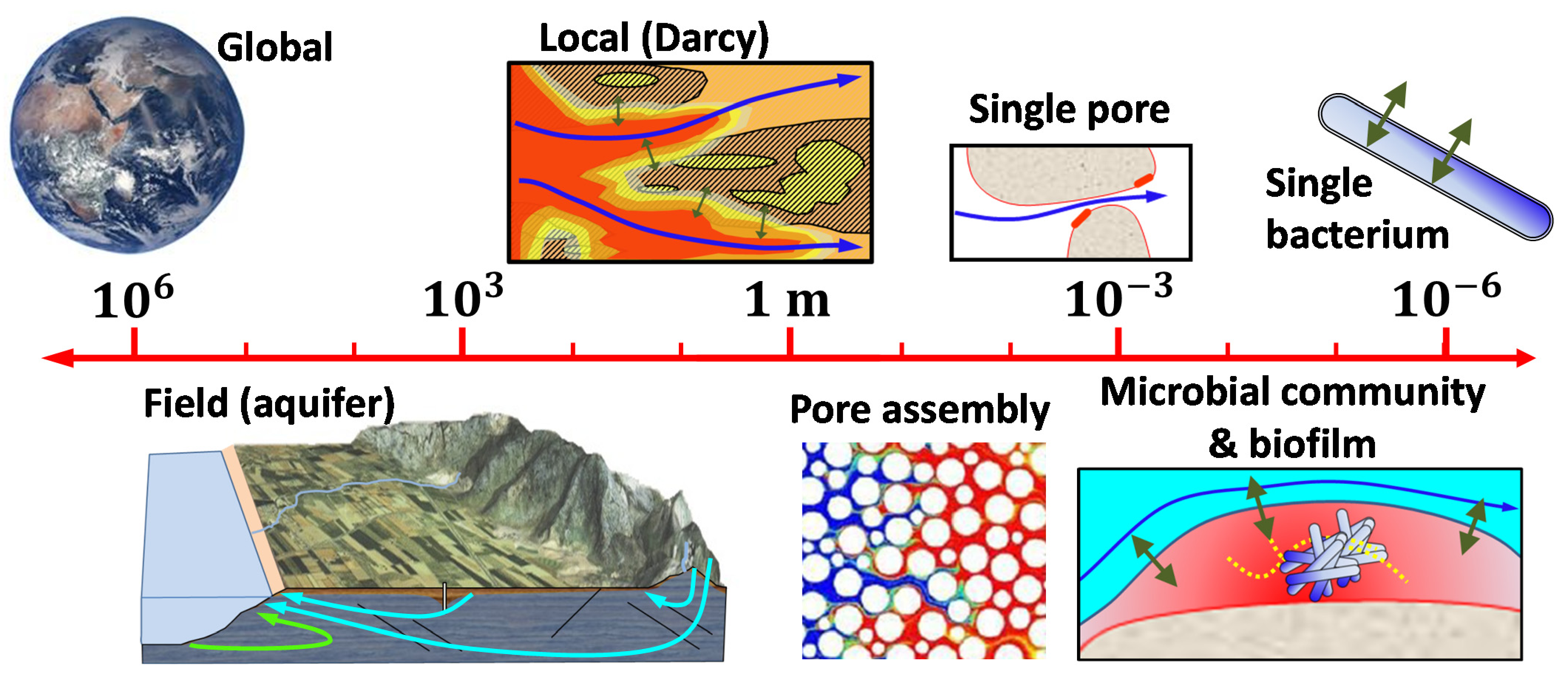
2	Diffusion controls microscales; advection controls macroscales; the Peclet number is ambiguous
	The ADE characteristic length is D/q. Pe is not a property of the equation, but of one model scale. Several scales may be relevant in practice. Better compare these to D/q, which leads to the above statement for diffusion coefficients and GW flux (Section 3.2).
3	It is important to select the appropriate set of species and reactions
	Selection of species and reactions requires understanding geochemistry, where it can be helped by speciation codes (Section 2.2), and biochemistry, where selection of biological reaction is more difficult, though at least they should be thermodynamically favorable (Section 5.1).
4	Equilibrium reactions reduce the size and complexity of RT problems
	The number of components, or the number of transport equations to be solved, equals the number of species minus the number of equilibrium reactions (Section 2.2 and 2.3).
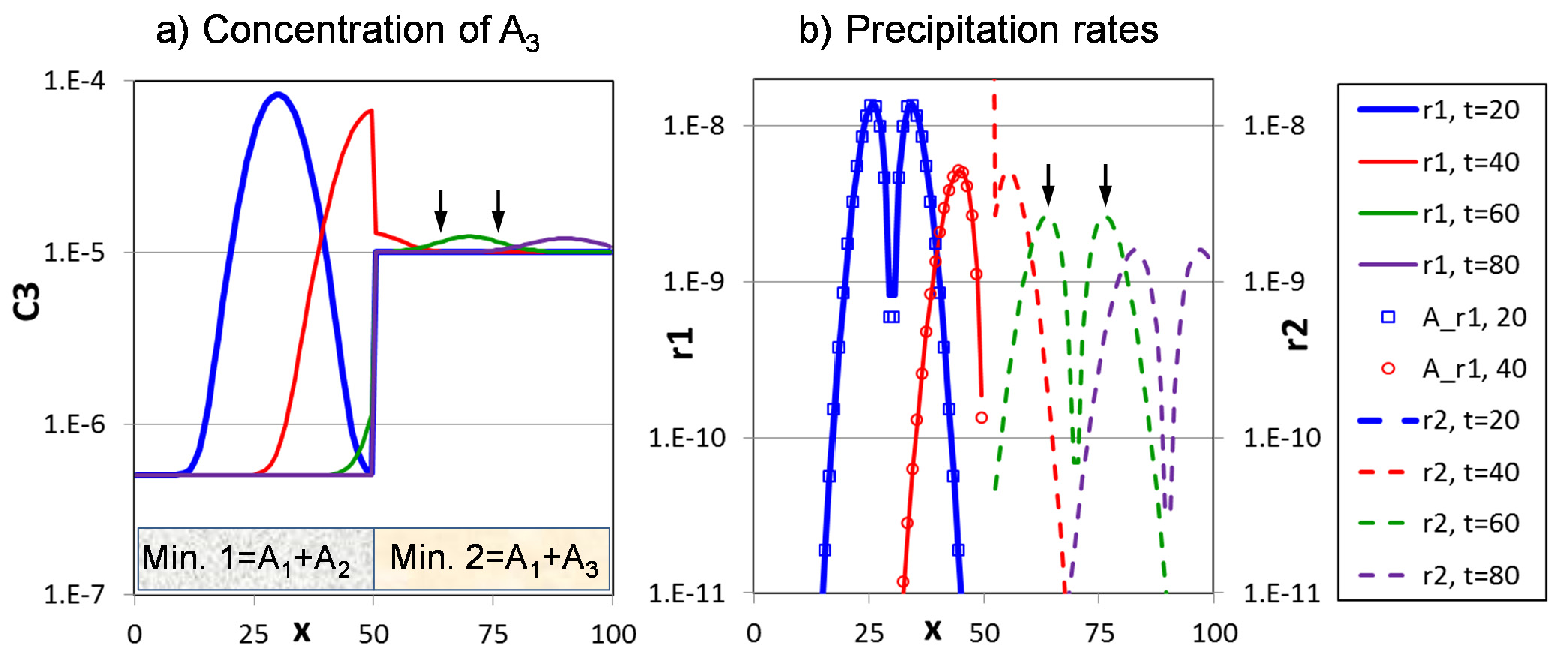
5	Mineral zones variations lead to sharp fronts in aqueous chemistry
	The set of equilibrium reactions in any subdomain (loosely, mineral zone) determines the chemical system and the equations that need to be solved (set of mass action laws, components, etc.) and, thus, water chemistry (Section 3.3). Note that varying microbial communities may have a similar effect (redox zonation).
6	Each species travels at a different velocity
	Solid species do not move, whereas aqueous species do. Exchanging species are retarded with respect to wa-ter while mobilizing others (Section 3.1). This hinders the accuracy of Lagrangian methods and leads to non-linear dependence between total concentration of a component ($u$) and its aqueous part ($u_a$) in the transport equation (Equation (22)).
7	Kinetics are important and complex
	Equilibrium constants are well-known, the gist of RT often lies on the adopted kinetic laws and their parameters (Section 2.2 and Section 5). Since kinetic rates are often variable, beware of the Damköhler number (Section 5.2).
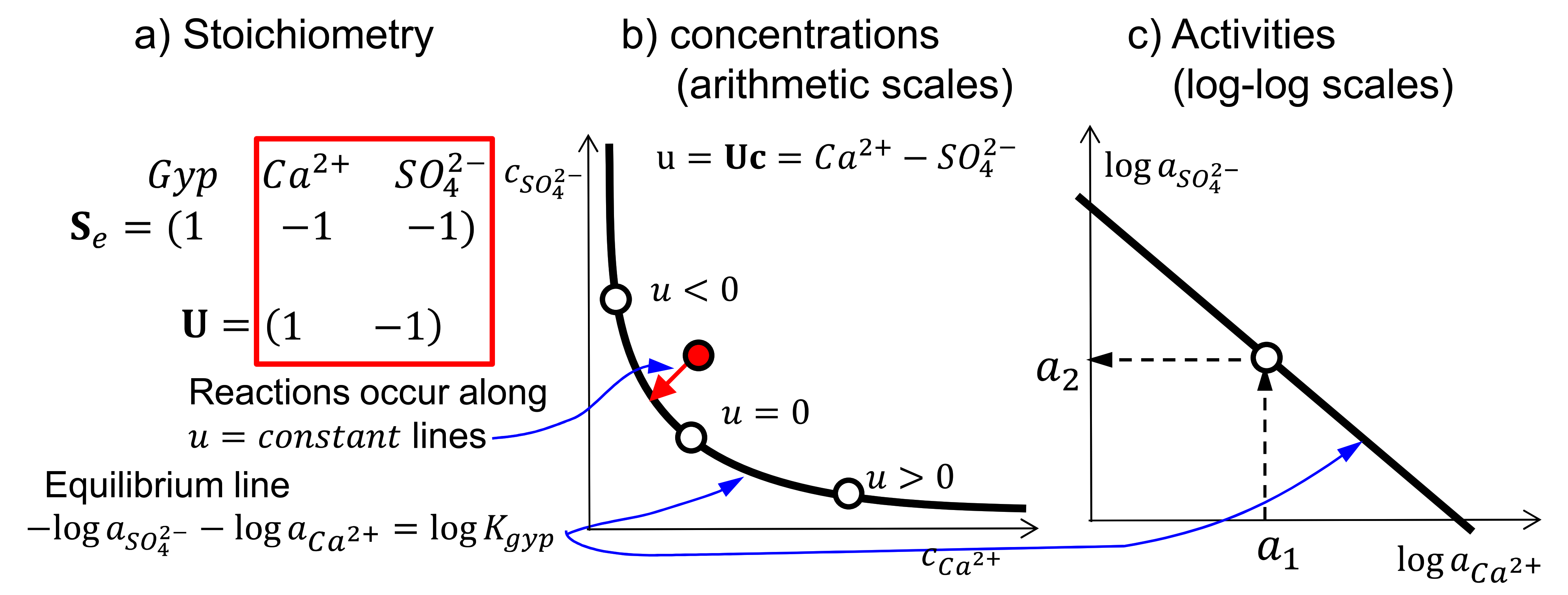
8	The rate of fast reactions is controlled by mixing and access to reaction sites
	For cases with only aqueous and mineral reaction in equilibrium reaction rates can be expressed by Equation (32), which implies that mixing rates need to be accurately modeled for accurate RT.
9	Solutes are displaced by advection, spread by dispersion, diluted by mixing
	The ADE is a poor representation of transport as it does not distinguish dispersion from mixing. This has been acknowledged for conservative transport, but it is even more relevant for RT.
10	Biochemical reactions involve microorganisms
	Microorganisms mean complex kinetic rate laws. Moreover, they can create biofilms that alter heterogeneity and flow and transport characteristics of the porous media. Yet, accurate biochemistry requires acknowledging both microbial communities and biofilms.
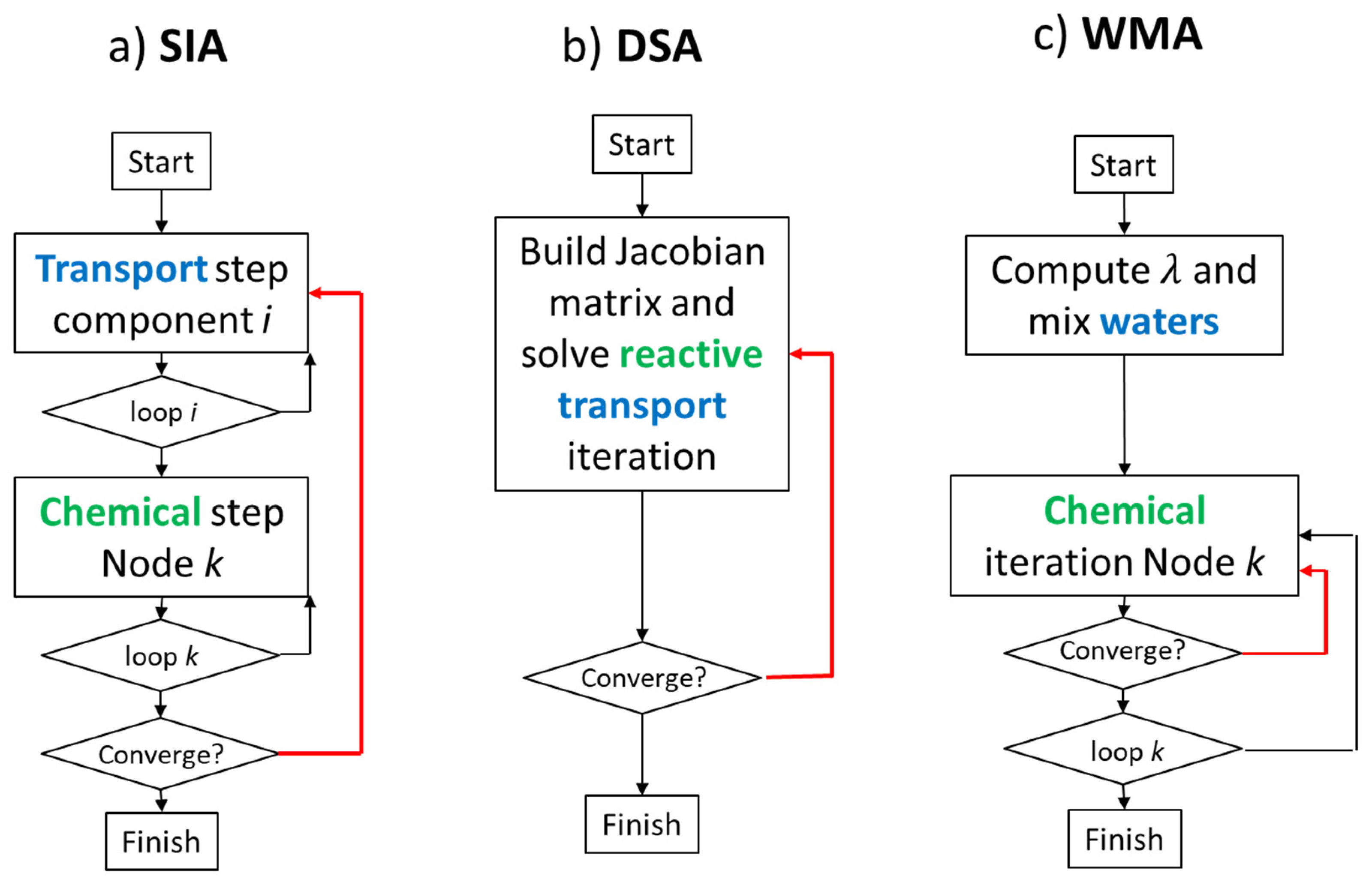
11	Select an appropriate solution method for efficient and accurate RT
	Solution methods may control the way mixing, and thus fast reactions, are represented, whether chemical localization can be reproduced, etc. Therefore, not only for efficiency, but also for conceptual consistence, an appropriate solution method needs to be adopted.

Table 1. Proposed list of basic RT conceptual issues.

No.	Conceptual Issue
1	RT is multidisciplinary and requires interdisciplinarity
	RT requires not only expertise on flow, hydrogeochemistry, biology, transport or numerics, but also close interaction between experts to understand interactions among processes.
2	Diffusion controls microscales; advection controls macroscales; the Peclet number is ambiguous
	The ADE characteristic length is D/q. Pe is not a property of the equation, but of one model scale. Several scales may be relevant in practice. Better compare these to D/q, which leads to the above statement for diffusion coefficients and GW flux (Section 3.2).
3	It is important to select the appropriate set of species and reactions
	Selection of species and reactions requires understanding geochemistry, where it can be helped by speciation codes (Section 2.2), and biochemistry, where selection of biological reaction is more difficult, though at least they should be thermodynamically favorable (Section 5.1).
4	Equilibrium reactions reduce the size and complexity of RT problems
	The number of components, or the number of transport equations to be solved, equals the number of species minus the number of equilibrium reactions (Section 2.2 and 2.3).
5	Mineral zones variations lead to sharp fronts in aqueous chemistry
	The set of equilibrium reactions in any subdomain (loosely, mineral zone) determines the chemical system and the equations that need to be solved (set of mass action laws, components, etc.) and, thus, water chemistry (Section 3.3). Note that varying microbial communities may have a similar effect (redox zonation).
6	Each species travels at a different velocity
	Solid species do not move, whereas aqueous species do. Exchanging species are retarded with respect to wa-ter while mobilizing others (Section 3.1). This hinders the accuracy of Lagrangian methods and leads to non-linear dependence between total concentration of a component ($u$) and its aqueous part ($u_a$) in the transport equation (Equation (22)).
7	Kinetics are important and complex
	Equilibrium constants are well-known, the gist of RT often lies on the adopted kinetic laws and their parameters (Section 2.2 and Section 5). Since kinetic rates are often variable, beware of the Damköhler number (Section 5.2).
8	The rate of fast reactions is controlled by mixing and access to reaction sites
	For cases with only aqueous and mineral reaction in equilibrium reaction rates can be expressed by Equation (32), which implies that mixing rates need to be accurately modeled for accurate RT.
9	Solutes are displaced by advection, spread by dispersion, diluted by mixing
	The ADE is a poor representation of transport as it does not distinguish dispersion from mixing. This has been acknowledged for conservative transport, but it is even more relevant for RT.
10	Biochemical reactions involve microorganisms
	Microorganisms mean complex kinetic rate laws. Moreover, they can create biofilms that alter heterogeneity and flow and transport characteristics of the porous media. Yet, accurate biochemistry requires acknowledging both microbial communities and biofilms.
11	Select an appropriate solution method for efficient and accurate RT
	Solution methods may control the way mixing, and thus fast reactions, are represented, whether chemical localization can be reproduced, etc. Therefore, not only for efficiency, but also for conceptual consistence, an appropriate solution method needs to be adopted.

References

1. Li, L. Watershed Reactive Transport. Rev. Mineral. Geochem. 2019, 85, 381–418. [Google Scholar] [CrossRef] [Green Version]
2. Valhondo, C.; Martinez-Landa, L.; Carrera, J.; Ayora, C.; Nödler, K.; Licha, T. Evaluation of EOC removal processes during artificial recharge through a reactive barrier. Sci. Total Environ. 2018, 612, 985–994. [Google Scholar] [CrossRef] [PubMed]
3. Barbieri, M.; Carrera, J.; Sanchez-Vila, X.; Ayora, C.; Cama, J.; Köck-Schulmeyer, M.; López De Alda, M.; Barceló, D.; Tobella Brunet, J.; Hernández García, M. Microcosm experiments to control anaerobic redox conditions when studying the fate of organic micropollutants in aquifer material. J. Contam. Hydrol. 2011, 126, 330–345. [Google Scholar] [CrossRef] [PubMed]
4. Šimůnek, J.; van Genuchten, M.T.; Šejna, M. Development and Applications of the HYDRUS and STANMOD Software Packages and Related Codes. Vadose Zo. J. 2008, 7, 587–600. [Google Scholar] [CrossRef] [Green Version]
5. Werner, A.D.; Bakker, M.; Post, V.E.A.; Vandenbohede, A.; Lu, C.; Ataie-Ashtiani, B.; Simmons, C.T.; Barry, D.A. Seawater intrusion processes, investigation and management: Recent advances and future challenges. Adv. Water Resour. 2013, 51, 3–26. [Google Scholar] [CrossRef]
6. Berkowitz, B.; Cortis, A.; Dentz, M.; Scher, H. Modeling Non-fickian transport in geological formations as a continuous time random walk. Rev. Geophys. 2006, 44, 1–49. [Google Scholar] [CrossRef] [Green Version]
7. Liger, E.; Charlet, L.; Van Cappellen, P. Surface catalysis of uranium(VI) reduction by iron(II). Geochim. Cosmochim. Acta 1999, 63, 2939–2955. [Google Scholar] [CrossRef]
8. Rubin, J.; James, R.V. Dispersion-affected transport of reacting solutes in saturated porous media: Galerkin Method applied to equilibrium-controlled exchange in unidirectional steady water flow. Water Resour. Res. 1973, 9, 1332–1356. [Google Scholar] [CrossRef]
9. Grovea, D.B.; Wood, W.W. Prediction and Field Verification of Subsurface-Water Quality Changes During Artificial Recharge, Lubbock, Texas. Groundwater 1979, 17, 250–257. [Google Scholar] [CrossRef]
10. Lichtner, P.C. Continuum model for simultaneous chemical reactions and mass transport in hydrothermal systems. Geochim. Cosmochim. Acta 1985, 49, 779–800. [Google Scholar] [CrossRef]
11. Cao, T.; Han, D.; Song, X. Past, present, and future of global seawater intrusion research: A bibliometric analysis. J. Hydrol. 2021, 603, 126844. [Google Scholar] [CrossRef]
12. Rubin, J. Transport of reacting solutes in porous media: Relation between mathematical nature of problem formulation and chemical nature of reactions. Water Resour. Res. 1983, 19, 1231–1252. [Google Scholar] [CrossRef]
13. Steefel, C.I.; DePaolo, D.J.; Lichtner, P.C. Reactive transport modeling: An essential tool and a new research approach for the Earth sciences. Earth Planet. Sci. Lett. 2005, 240, 539–558. [Google Scholar] [CrossRef]
14. Gaus, I. Role and impact of CO2-rock interactions during CO2 storage in sedimentary rocks. Int. J. Greenh. Gas Control 2010, 4, 73–89. [Google Scholar] [CrossRef]
15. Liu, P.; Zhang, T.; Sun, S. A tutorial review of reactive transport modeling and risk assessment for geologic CO2 sequestration. Comput. Geosci. 2019, 127, 1–11. [Google Scholar] [CrossRef]
16. Cama, J.; Soler, J.M.; Ayora, C. Acid Water–Rock–Cement Interaction and Multicomponent Reactive Transport Modeling. Rev. Mineral. Geochem. 2019, 85, 459–498. [Google Scholar] [CrossRef]
17. Amos, R.T.; Blowes, D.W.; Bailey, B.L.; Sego, D.C.; Smith, L.; Ritchie, A.I.M. Waste-rock hydrogeology and geochemistry. Appl. Geochem. 2015, 57, 140–156. [Google Scholar] [CrossRef]
18. Cumberland, S.A.; Douglas, G.; Grice, K.; Moreau, J.W. Uranium mobility in organic matter-rich sediments: A review of geological and geochemical processes. Earth-Sci. Rev. 2016, 159, 160–185. [Google Scholar] [CrossRef] [Green Version]
19. Liang, S.-Y.; Lin, W.-S.; Chen, C.-P.; Liu, C.-W.; Fan, C. A Review of Geochemical Modeling for the Performance Assessment of Radioactive Waste Disposal in a Subsurface System. Appl. Sci. 2021, 11, 5879. [Google Scholar] [CrossRef]
20. Gaucher, E.C.; Blanc, P. Cement/clay interactions—A review: Experiments, natural analogues, and modeling. Waste Manag. 2006, 26, 776–788. [Google Scholar] [CrossRef] [Green Version]
21. MacQuarrie, K.T.B.; Mayer, K.U. Reactive transport modeling in fractured rock: A state-of-the-science review. Earth-Sci. Rev. 2005, 72, 189–227. [Google Scholar] [CrossRef]
22. Dignac, M.-F.; Derrien, D.; Barré, P.; Barot, S.; Cécillon, L.; Chenu, C.; Chevallier, T.; Freschet, G.T.; Garnier, P.; Guenet, B.; et al. Increasing soil carbon storage: Mechanisms, effects of agricultural practices and proxies. A review. Agron. Sustain. Dev. 2017, 37, 14. [Google Scholar] [CrossRef] [Green Version]
23. Li, L.; Maher, K.; Navarre-Sitchler, A.; Druhan, J.; Meile, C.; Lawrence, C.; Moore, J.; Perdrial, J.; Sullivan, P.; Thompson, A.; et al. Expanding the role of reactive transport models in critical zone processes. Earth-Sci. Rev. 2017, 165, 280–301. [Google Scholar] [CrossRef] [Green Version]
24. Arndt, S.; Jørgensen, B.B.; LaRowe, D.E.; Middelburg, J.J.; Pancost, R.D.; Regnier, P. Quantifying the degradation of organic matter in marine sediments: A review and synthesis. Earth-Sci. Rev. 2013, 123, 53–86. [Google Scholar] [CrossRef]
25. Regnier, P.; Dale, A.W.; Arndt, S.; LaRowe, D.E.; Mogollón, J.; Van Cappellen, P. Quantitative analysis of anaerobic oxidation of methane (AOM) in marine sediments: A modeling perspective. Earth-Sci. Rev. 2011, 106, 105–130. [Google Scholar] [CrossRef]
26. Langergraber, G. Modeling of Processes in Subsurface Flow Constructed Wetlands: A Review. Vadose Zo. J. 2008, 7, 830–842. [Google Scholar] [CrossRef] [Green Version]
27. Patil, V.; McPherson, B.J. Modeling Coupled Reactive Transport through Fault Zones: A Critical Review. Environ. Eng. Sci. 2021, 38, 165–180. [Google Scholar] [CrossRef]
28. Deng, H.; Navarre-Sitchler, A.; Heil, E.; Peters, C. Addressing Water and Energy Challenges with Reactive Transport Modeling. Environ. Eng. Sci. 2021, 38, 109–114. [Google Scholar] [CrossRef]
29. Ajayi, T.; Gupta, I. A review of reactive transport modeling in wellbore integrity problems. J. Pet. Sci. Eng. 2019, 175, 785–803. [Google Scholar] [CrossRef]
30. Abd, A.S.; Abushaikha, A.S. Reactive transport in porous media: A review of recent mathematical efforts in modeling geochemical reactions in petroleum subsurface reservoirs. SN Appl. Sci. 2021, 3, 401. [Google Scholar] [CrossRef]
31. Hommel, J.; Coltman, E.; Class, H. Porosity–Permeability Relations for Evolving Pore Space: A Review with a Focus on (Bio-)geochemically Altered Porous Media. Transp. Porous Media 2018, 124, 589–629. [Google Scholar] [CrossRef] [Green Version]
32. Molins, S.; Knabner, P. Multiscale Approaches in Reactive Transport Modeling. Rev. Mineral. Geochem. 2019, 85, 27–48. [Google Scholar] [CrossRef] [Green Version]
33. Ladd, A.J.C.; Szymczak, P. Reactive Flows in Porous Media: Challenges in Theoretical and Numerical Methods. Annu. Rev. Chem. Biomol. Eng. 2021, 12, 543–571. [Google Scholar] [CrossRef]
34. Seigneur, N.; Mayer, K.U.; Steefel, C.I. Reactive Transport in Evolving Porous Media. Rev. Mineral. Geochem. 2019, 85, 197–238. [Google Scholar] [CrossRef] [Green Version]
35. Zhang, R.; Min, T.; Liu, Y.; Chen, L.; Tao, W.Q. Pore-scale study of effects of different Pt loading reduction schemes on reactive transport processes in catalyst layers of proton exchange membrane fuel cells. Int. J. Hydrogen Energy 2021, 46, 20037–20053. [Google Scholar] [CrossRef]
36. Meakin, P.; Tartakovsky, A.M. Modeling and simulation of pore-scale multiphase fluid flow and reactive transport in fractured and porous media. Rev. Geophys. 2009, 47, 1–47. [Google Scholar] [CrossRef]
37. Xiong, Q.; Baychev, T.G.; Jivkov, A.P. Review of pore network modelling of porous media: Experimental characterisations, network constructions and applications to reactive transport. J. Contam. Hydrol. 2016, 192, 101–117. [Google Scholar] [CrossRef]
38. Yeh, G.T.; Tripathi, V.S. A critical evaluation of recent developments in hydrogeochemical transport models of reactive multichemical components. Water Resour. Res. 1989, 25, 93–108. [Google Scholar] [CrossRef]
39. Saaltink, M.W.; Carrera, J.; Ayora, C. On the behavior of approaches to simulate reactive transport. J. Contam. Hydrol. 2001, 48, 213–235. [Google Scholar] [CrossRef]
40. Steefel, C.I.; Appelo, C.A.J.; Arora, B.; Jacques, D.; Kalbacher, T.; Kolditz, O.; Lagneau, V.; Lichtner, P.C.; Mayer, K.U.; Meeussen, J.C.L.; et al. Reactive Transport Codes for Subsurface Environmental Simulation; Springer: Berlin/Heidelberg, Germany, 2015; Volume 19, ISBN 1059601494. [Google Scholar]
41. Dai, Z.; Samper, J. Inverse problem of multicomponent reactive chemical transport in porous media: Formulation and applications. Water Resour. Res. 2004, 40, 40. [Google Scholar] [CrossRef]
42. Majdalani, S.; Fahs, M.; Carrayrou, J.; Ackerer, P. Reactive transport parameter estimation: Genetic algorithm vs. Monte carlo approach. AIChE J. 2009, 55, 1959–1968. [Google Scholar] [CrossRef]
43. Torlapati, J.; Clement, T.P. Using Parallel Genetic Algorithms for Estimating Model Parameters in Complex Reactive Transport Problems. Processes 2019, 7, 640. [Google Scholar] [CrossRef] [Green Version]
44. Bear, J. Dynamics of Fluids in Porous Media (Dover Civil and Mechanical Engineering); Elsevier: New York, NY, USA, 1972. [Google Scholar]
45. Olivella, S.; Carrera, J.; Gens, A.; Alonso, E.E. Nonisothermal multiphase flow of brine and gas through saline media. Transp. Porous Media 1994, 15, 271–293. [Google Scholar] [CrossRef]
46. Cordes, C.; Kinzelbach, W. Continuous groundwater velocity fields and path lines in linear, bilinear, and trilinear finite elements. Water Resour. Res. 1992, 28, 2903–2911. [Google Scholar] [CrossRef]
47. Saaltink, M.W.; Batlle, F.; Ayora, C.; Carrera, J.; Olivella, S. RETRASO, a code for modeling reactive transport in saturated and unsaturated porous media. Geol. Acta 2004, 2, 235–251. [Google Scholar] [CrossRef]
48. Friedly, J.C.; Rubin, J. Solute transport with multiple equilibrium-controlled or kinetically controlled chemical reactions. Water Resour. Res. 1992, 28, 1935–1953. [Google Scholar] [CrossRef]
49. Prigogine, I.; Defay, R. On the Number of Independent Constituents and the Phase Rule. J. Chem. Phys. 1947, 15, 614–615. [Google Scholar] [CrossRef]
50. Lasaga, A.C. Kinetic Theory in the Earth Sciences; Princeton University Press: Princeton, NJ, USA, 2014. [Google Scholar]
51. Appelo, C.A.J.; Postma, D. Geochemistry, Groundwater and Pollution, 2nd ed.; CRC Press: London, UK, 2005; Volume 59. [Google Scholar]
52. Wolery, T.J. Calculation of Chemical Equilibrium between Aqueous Solution and Minerals: The EQ 3/6 Software Package; Lawrence Livermore Laboratory, University of California: Livermore, CA, USA, 1979. [Google Scholar]
53. Parkhurst, D.L.; Thorstenson, D.C.; Plummer, N. PHREEQE: A Computer Program for Geochemical Calculations; U.S. Geological Survey, Water Resources Division: Reston, VA, USA, 1980.
54. Krupka, K.M.; Cantrell, K.J.; McGrail, B.P. Thermodynamic Data for Geochemical Modeling of Carbonate Reactions Associated with CO2 Sequestration–Literature Review; U.S. Department of Energy: Washington, DC, USA, 2010.
55. Blanc, P.; Vieillard, P.; Gailhanou, H.; Gaboreau, S.; Marty, N.; Claret, F.; Madé, B.; Giffaut, E. ThermoChimie database developments in the framework of cement/clay interactions. Appl. Geochem. 2015, 55, 95–107. [Google Scholar] [CrossRef]
56. Martinez, J.S.; Santillan, E.-F.; Bossant, M.; Costa, D.; Ragoussi, M.-E. The new electronic database of the NEA Thermochemical Database Project. Appl. Geochem. 2019, 107, 159–170. [Google Scholar] [CrossRef]
57. Palandri, J.L.; Kharaka, Y.K. A Compilation of Rate Parameters of Water-Mineral Interaction Kinetics for Application to Geochemical Modeling; U.S. Geological Survey: Reston, VA, USA, 2004.
58. Marty, N.C.M.; Claret, F.; Lassin, A.; Tremosa, J.; Blanc, P.; Madé, B.; Giffaut, E.; Cochepin, B.; Tournassat, C. A database of dissolution and precipitation rates for clay-rocks minerals. Appl. Geochem. 2015, 55, 108–118. [Google Scholar] [CrossRef]
59. Li, L.; Steefel, C.I.; Kowalsky, M.B.; Englert, A.; Hubbard, S.S. Effects of physical and geochemical heterogeneities on mineral transformation and biomass accumulation during biostimulation experiments at Rifle, Colorado. J. Contam. Hydrol. 2010, 112, 45–63. [Google Scholar] [CrossRef]
60. Kim, S.; Gindulyte, A.; Zhang, J.; Thiessen, P.A.; Bolton, E.E. PubChem Periodic Table and Element pages: Improving access to information on chemical elements from authoritative sources. Chem. Teach. Int. 2021, 3, 57–65. [Google Scholar] [CrossRef]
61. Molins, S.; Carrera, J.; Ayora, C.; Saaltink, M.W. A formulation for decoupling components in reactive transport problems. Water Resour. Res. 2004, 40, W103011–W1030113. [Google Scholar] [CrossRef]
62. Steefel, C.I.; MacQuarrie, K.T.B. Approaches to modeling reactive transport in porous media. Rev. Mineral. Geochem. 1996, 34, 83–125. [Google Scholar]
63. Saaltink, M.W.; Ayora, C.; Carrera, J. A mathematical formulation for reactive transport that eliminates mineral concentrations. Water Resour. Res. 1998, 34, 1649–1656. [Google Scholar] [CrossRef]
64. Saaltink, M.W.; Carrera Ramirez, J.; Ayora, C. Numerical solutions of reactive transport equations. In Geochemical Modeling of Groundwater, Vadose and Geothermal Systems; CRC Press: Boca Raton, FL, USA, 2011. [Google Scholar]
65. Marinoni, M.; Carrayrou, J.; Lucas, Y.; Ackerer, P. Thermodynamic equilibrium solutions through a modified Newton Raphson method. AIChE J. 2017, 63, 1246–1262. [Google Scholar] [CrossRef]
66. Carrayrou, J.; Bertagnolli, C.; Fahs, M. Algorithms for activity correction models for geochemical speciation and reactive transport modeling. AIChE J. 2022, 68, e17391. [Google Scholar] [CrossRef]
67. Parkhurst, D.L.; Appelo, C.A.J. PHREEQC (Version 3)—A Computer Program for Speciation, Batch-Reaction, One-Dimensional Transport, and Inverse Geochemical Calculations; U.S. Geological Survey: Reston, VA, USA, 2013.
68. Bea, S.A.; Carrera, J.; Ayora, C.; Batlle, F.; Saaltink, M.W. CHEPROO: A Fortran 90 object-oriented module to solve chemical processes in Earth Science models. Comput. Geosci. 2009, 35, 1098–1112. [Google Scholar] [CrossRef]
69. Kulik, D.A.; Wagner, T.; Dmytrieva, S.V.; Kosakowski, G.; Hingerl, F.F.; Chudnenko, K.V.; Berner, U.R. GEM-Selektor geochemical modeling package: Revised algorithm and GEMS3K numerical kernel for coupled simulation codes. Comput. Geosci. 2013, 17, 1–24. [Google Scholar] [CrossRef] [Green Version]
70. Leal, A.M.M.; Kyas, S.; Kulik, D.A.; Saar, M.O. Accelerating Reactive Transport Modeling: On-Demand Machine Learning Algorithm for Chemical Equilibrium Calculations. Transp. Porous Media 2020, 133, 161–204. [Google Scholar] [CrossRef]
71. Kräutle, S.; Knabner, P. A new numerical reduction scheme for fully coupled multicomponent transport-reaction problems in porous media. Water Resour. Res. 2005, 41, 1–17. [Google Scholar] [CrossRef] [Green Version]
72. Kräutle, S.; Knabner, P. A reduction scheme for coupled multicomponent transport-reaction problems in porous media: Generalization to problems with heterogeneous equilibrium reactions. Water Resour. Res. 2007, 43, 1–15. [Google Scholar] [CrossRef]
73. De Simoni, M.; Carrera, J.; Sánchez-Vila, X.; Guadagnini, A. A procedure for the solution of multicomponent reactive transport problems. Water Resour. Res. 2005, 41, 1–16. [Google Scholar] [CrossRef]
74. Michael, H.A.; Charette, M.A.; Harvey, C.F. Patterns and variability of groundwater flow and radium activity at the coast: A case study from Waquoit Bay, Massachusetts. Mar. Chem. 2011, 127, 100–114. [Google Scholar] [CrossRef]
75. Moore, W.S. Determining coastal mixing rates using radium isotopes. Cont. Shelf Res. 2000, 20, 1993–2007. [Google Scholar] [CrossRef]
76. Appelo, C.A.J.; Van Der Weiden, M.J.J.; Tournassat, C.; Charlet, L. Surface Complexation of Ferrous Iron and Carbonate on Ferrihydrite and the Mobilization of Arsenic. Environ. Sci. Technol. 2002, 36, 3096–3103. [Google Scholar] [CrossRef] [PubMed]
77. Valocchi, A.J.; Street, R.L.; Roberts, P.V. Transport of ion-exchanging solutes in groundwater: Chromatographic theory and field simulation. Water Resour. Res. 1981, 17, 1517–1527. [Google Scholar] [CrossRef]
78. Charbeneau, R.J. Groundwater contaminant transport with adsorption and ion exchange chemistry: Method of characteristics for the case without dispersion. Water Resour. Res. 1981, 17, 705–713. [Google Scholar] [CrossRef]
79. Appelo, C.A.J. Some Calculations on Multicomponent Transport with Cation Exchange in Aquifers. Groundwater 1994, 32, 968–975. [Google Scholar] [CrossRef]
80. Appelo, C.A.J. Cation and proton exchange, pH variations, and carbonate reactions in a freshening aquifer. Water Resour. Res. 1994, 30, 2793–2805. [Google Scholar] [CrossRef]
81. Steefel, C.I.; Carroll, S.; Zhao, P.; Roberts, S. Cesium migration in Hanford sediment: A multisite cation exchange model based on laboratory transport experiments. J. Contam. Hydrol. 2003, 67, 219–246. [Google Scholar] [CrossRef]
82. Tournassat, C.; Gailhanou, H.; Crouzet, C.; Braibant, G.; Gautier, A.; Lassin, A.; Blanc, P.; Gaucher, E.C. Two cation exchange models for direct and inverse modelling of solution major cation composition in equilibrium with illite surfaces. Geochim. Cosmochim. Acta 2007, 71, 1098–1114. [Google Scholar] [CrossRef] [Green Version]
83. Bradbury, M.H.; Baeyens, B. A generalised sorption model for the concentration dependent uptake of caesium by argillaceous rocks. J. Contam. Hydrol. 2000, 42, 141–163. [Google Scholar] [CrossRef]
84. Shiri, J.; Keshavarzi, A.; Kisi, O.; Iturraran-Viveros, U.; Bagherzadeh, A.; Mousavi, R.; Karimi, S. Modeling soil cation exchange capacity using soil parameters: Assessing the heuristic models. Comput. Electron. Agric. 2017, 135, 242–251. [Google Scholar] [CrossRef]
85. Kashi, H.; Emamgholizadeh, S.; Ghorbani, H. Estimation of Soil Infiltration and Cation Exchange Capacity Based on Multiple Regression, ANN (RBF, MLP), and ANFIS Models. Commun. Soil Sci. Plant Anal. 2014, 45, 1195–1213. [Google Scholar] [CrossRef]
86. Möri, A.; Alexander, W.R.; Geckeis, H.; Hauser, W.; Schäfer, T.; Eikenberg, J.; Fierz, T.; Degueldre, C.; Missana, T. The colloid and radionuclide retardation experiment at the Grimsel Test Site: Influence of bentonite colloids on radionuclide migration in a fractured rock. Colloids Surfaces A Physicochem. Eng. Asp. 2003, 217, 33–47. [Google Scholar] [CrossRef]
87. Painter, S.; Cvetkovic, V.; Turner, D.R. Effect of heterogeneity on radionuclide retardation in the alluvial aquifer near Yucca Mountain, Nevada. Ground Water 2001, 39, 326–338. [Google Scholar] [CrossRef]
88. Trinchero, P.; Cvetkovic, V.; Selroos, J.-O.; Bosbach, D.; Deissmann, G. Upscaling of radionuclide transport and retention in crystalline rocks exhibiting micro-scale heterogeneity of the rock matrix. Adv. Water Resour. 2020, 142, 103644. [Google Scholar] [CrossRef]
89. Domenech, C.; Arcos, D.; Sellin, P. Review on Cation Exchange Selectivity Coefficients for MX-80 Bentonite. 2005. Available online: https://inis.iaea.org/search/search.aspx?orig_q=RN:38093000 (accessed on 22 November 2021).
90. White, A.F.; Peterson, M.L. Role of Reactive-Surface-Area Characterization in Geochemical Kinetic Models. In Chemical Modeling of Aqueous Systems II; ACS Symposium Series; American Chemical Society: Washington, DC, USA, 1990; Volume 416, pp. 35–461. ISBN 9780841217294. [Google Scholar]
91. Maher, K.; Steefel, C.I.; DePaolo, D.J.; Viani, B.E. The mineral dissolution rate conundrum: Insights from reactive transport modeling of U isotopes and pore fluid chemistry in marine sediments. Geochim. Cosmochim. Acta 2006, 70, 337–363. [Google Scholar] [CrossRef]
92. Valhondo, C.; Carrera, J.; Ayora, C.; Tubau, I.; Martinez-Landa, L.; Nödler, K.; Licha, T. Characterizing redox conditions and monitoring attenuation of selected pharmaceuticals during artificial recharge through a reactive layer. Sci. Total Environ. 2015, 512–513, 240–250. [Google Scholar] [CrossRef]
93. Sanchez-Vila, X.; Donado, L.D.; Guadagnini, A.; Carrera, J. A solution for multicomponent reactive transport under equilibrium and kinetic reactions. Water Resour. Res. 2010, 46, 1–13. [Google Scholar] [CrossRef]
94. Wigley, T.M.L.; Plummer, L.N. Mixing of carbonate waters. Geochim. Cosmochim. Acta 1976, 40, 989–995. [Google Scholar] [CrossRef]
95. Sanford, W.E.; Konikow, L.F. Simulation of calcite dissolution and porosity changes in saltwater mixing zones in coastal aquifers. Water Resour. Res. 1989, 25, 655–667. [Google Scholar] [CrossRef]
96. Rezaei, M.; Sanz, E.; Raeisi, E.; Ayora, C.; Vázquez-Suñé, E.; Carrera, J. Reactive transport modeling of calcite dissolution in the fresh-salt water mixing zone. J. Hydrol. 2005, 311, 282–298. [Google Scholar] [CrossRef]
97. Kitanidis, P.K. The concept of the Dilution Index. Water Resour. Res. 1994, 30, 2011–2026. [Google Scholar] [CrossRef]
98. Carrera, J.; Vázquez-Suñé, E.; Castillo, O.; Sánchez-Vila, X. A methodology to compute mixing ratios with uncertain end-members. Water Resour. Res. 2004, 40. [Google Scholar] [CrossRef] [Green Version]
99. Valocchi, A.J. Validity of the Local Equilibrium Assumption for Modeling Sorbing Solute Transport through Homogeneous Soils. Water Resour. Res. 1985, 21, 808–820. [Google Scholar] [CrossRef]
100. Carrera, J. An overview of uncertainties in modelling groundwater solute transport. J. Contam. Hydrol. 1993, 13, 23–48. [Google Scholar] [CrossRef]
101. Lallemand-Barres, A.; Peaudecerf, P. Recherche des relations entre la valeur de la dispersivite macroscopique d’un milieu acquifere, ses autres characteristiques et les conditions de mesure. Bull. Bur. Rech. Geollogiques Minier. 1978, 3/4, 277–287. [Google Scholar]
102. Gelhar, L.W.; Welty, C.; Rehfeldt, K.R. A critical review of data on field-scale dispersion in aquifers. Water Resour. Res. 1992, 28, 1955–1974. [Google Scholar] [CrossRef]
103. Guimerà, J.; Carrera, J. A comparison of hydraulic and transport parameters measured in low- permeability fractured media. J. Contam. Hydrol. 2000, 41, 261–281. [Google Scholar] [CrossRef]
104. Sánchez-Vila, X.; Carrera, J. Directional effects on convergent flow tracer tests. Math. Geol. 1997, 29, 551–569. [Google Scholar] [CrossRef]
105. Neuman, S.P. On the tensorial nature of advective porosity. Adv. Water Resour. 2005, 28, 149–159. [Google Scholar] [CrossRef]
106. Gelhar, L.W.; Axness, C.L. Three-dimensional stochastic analysis of macrodispersion in aquifers. Water Resour. Res. 1983, 19, 161–180. [Google Scholar] [CrossRef]
107. Dagan, G. Solute transport in heterogeneous porous formations. J. Fluid Mech. 1984, 145, 151–177. [Google Scholar] [CrossRef]
108. Neuman, S.P.; Winter, C.L.; Newman, C.M. Stochastic theory of field-scale fickian dispersion in anisotropic porous media. Water Resour. Res. 1987, 23, 453–466. [Google Scholar] [CrossRef]
109. Frippiat, C.C.; Holeyman, A.E. A comparative review of upscaling methods for solute transport in heterogeneous porous media. J. Hydrol. 2008, 362, 150–176. [Google Scholar] [CrossRef]
110. Einstein, A. On the Motion of Small Particles Suspended in Liquids at Rest Required by the Molecular-Kinetic Theory of Heat. Ann. Phys. 1905, 17, 208. [Google Scholar]
111. Salamon, P.; Fernàndez-Garcia, D.; Gómez-Hernández, J.J. Modeling mass transfer processes using random walk particle tracking. Water Resour. Res. 2006, 42, 1–14. [Google Scholar] [CrossRef]
112. Noetinger, B.; Roubinet, D.; Russian, A.; Le Borgne, T.; Delay, F.; Dentz, M.; de Dreuzy, J.R.; Gouze, P. Random Walk Methods for Modeling Hydrodynamic Transport in Porous and Fractured Media from Pore to Reservoir Scale. Transp. Porous Media 2016, 115, 345–385. [Google Scholar] [CrossRef] [Green Version]
113. Fernàndez-Garcia, D.; Sanchez-Vila, X. Optimal reconstruction of concentrations, gradients and reaction rates from particle distributions. J. Contam. Hydrol. 2011, 120–121, 99–114. [Google Scholar] [CrossRef]
114. Sole-Mari, G.; Bolster, D.; Fernàndez-Garcia, D.; Sanchez-Vila, X. Particle density estimation with grid-projected and boundary-corrected adaptive kernels. Adv. Water Resour. 2019, 131, 103382. [Google Scholar] [CrossRef] [Green Version]
115. Tartakovsky, A.M.; Meakin, P.; Scheibe, T.D.; Eichler West, R.M. Simulations of reactive transport and precipitation with smoothed particle hydrodynamics. J. Comput. Phys. 2007, 222, 654–672. [Google Scholar] [CrossRef]
116. Tartakovsky, A.M.; Neuman, S.P. Effects of Peclet number on pore-scale mixing and channeling of a tracer and on directional advective porosity. Geophys. Res. Lett. 2008, 35, 1–4. [Google Scholar] [CrossRef]
117. Yoon, H.; Kang, Q.; Valocchi, A.J. Lattice boltzmann-based approaches for pore-scale reactive transport. Rev. Mineral. Geochem. 2015, 80, 393–431. [Google Scholar] [CrossRef]
118. Berkowitz, B.; Scher, H. Anomalous Transport in Random Fracture Networks. Phys. Rev. Lett. 1997, 79, 4038. [Google Scholar] [CrossRef]
119. Le Borgne, T.; Gouze, P. Non-Fickian dispersion in porous media: 2. Model validation from measurements at different scales. Water Resour. Res. 2008, 44, 1–10. [Google Scholar] [CrossRef] [Green Version]
120. Bijeljic, B.; Mostaghimi, P.; Blunt, M.J. Signature of non-fickian solute transport in complex heterogeneous porous media. Phys. Rev. Lett. 2011, 107, 20–23. [Google Scholar] [CrossRef] [PubMed] [Green Version]
121. Benson, D.A.; Wheatcraft, S.W.; Meerschaert, M.M. Application of a fractional advection-dispersion equation. Water Resour. Res. 2000, 36, 1403–1412. [Google Scholar] [CrossRef] [Green Version]
122. Schumer, R.; Benson, D.A.; Meerschaert, M.M.; Baeumer, B. Fractal mobile/immobile solute transport. Water Resour. Res. 2003, 39, 1–13. [Google Scholar] [CrossRef]
123. Oldham, K.B.; Spanier, J. The Fractional Calculus Theory and Applications of Differentiation and lntegration to Arbitrary Order; Elsevier: Amsterdam, The Netherlands, 1974; Volume 111. [Google Scholar]
124. Barker, J.A. A generalized radial flow model for hydraulic tests in fractured rock. Water Resour. Res. 1988, 24, 1796–1804. [Google Scholar] [CrossRef] [Green Version]
125. Carrera, J.; Sànchez-Vila, X.; Benet, I.; Medina, A.; Galarza, G.; Guimerà, J. On matrix diffusion: Formulations, solution methods and qualitative effects. Hydrogeol. J. 1998, 6, 178–190. [Google Scholar] [CrossRef]
126. Dentz, M.; Berkowitz, B. Transport behavior of a passive solute in continuous time random walks and multirate mass transfer. Water Resour. Res. 2003, 39, 1–20. [Google Scholar] [CrossRef]
127. Silva, O.; Carrera, J.; Dentz, M.; Kumar, S.; Alcolea, A.; Willmann, M. A general real-time formulation for multi-rate mass transfer problems. Hydrol. Earth Syst. Sci. 2009, 13, 1399–1411. [Google Scholar] [CrossRef] [Green Version]
128. Haggerty, R.; Gorelick, S.M. Multiple-Rate Mass Transfer for Modeling Diffusion and Surface Reactions in Media with Pore-Scale Heterogeneity. Water Resour. Res. 1995, 31, 2383–2400. [Google Scholar] [CrossRef]
129. Babey, T.; de Dreuzy, J.-R.; Casenave, C. Multi-Rate Mass Transfer (MRMT) models for general diffusive porosity structures. Adv. Water Resour. 2015, 76, 146–156. [Google Scholar] [CrossRef]
130. De Dreuzy, J.R.; Rapaport, A.; Babey, T.; Harmand, J. Influence of porosity structures on mixing-induced reactivity at chemical equilibrium in mobile/immobile Multi-Rate Mass Transfer (MRMT) and Multiple INteracting Continua (MINC) models. Water Resour. Res. 2013, 49, 8511–8530. [Google Scholar] [CrossRef] [Green Version]
131. Fernandez-Garcia, D.; Sanchez-Vila, X. Mathematical equivalence between time-dependent single-rate and multiratemass transfer models. Water Resour. Res. 2015, 51, 3166–3180. [Google Scholar] [CrossRef] [Green Version]
132. Battiato, I.; Tartakovsky, D.M.; Tartakovsky, A.M.; Scheibe, T. On breakdown of macroscopic models of mixing-controlled heterogeneous reactions in porous media. Adv. Water Resour. 2009, 32, 1664–1673. [Google Scholar] [CrossRef]
133. Battiato, I.; Tartakovsky, D.M.; Tartakovsky, A.M.; Scheibe, T.D. Hybrid models of reactive transport in porous and fractured media. Adv. Water Resour. 2011, 34, 1140–1150. [Google Scholar] [CrossRef]
134. Sadhukhan, S.; Gouze, P.; Dutta, T. A simulation study of reactive flow in 2-D involving dissolution and precipitation in sedimentary rocks. J. Hydrol. 2014, 519, 2101–2110. [Google Scholar] [CrossRef]
135. Scheibe, T.D.; Schuchardt, K.; Agarwal, K.; Chase, J.; Yang, X.; Palmer, B.J.; Tartakovsky, A.M.; Elsethagen, T.; Redden, G. Hybrid multiscale simulation of a mixing-controlled reaction. Adv. Water Resour. 2015, 83, 228–239. [Google Scholar] [CrossRef] [Green Version]
136. Tartakovsky, A.M.; Tartakovsky, D.M.; Scheibe, T.D.; Meakin, P. Hybrid simulations of reaction-diffusion systems in porous media. SIAM J. Sci. Comput. 2008, 30, 2799–2816. [Google Scholar] [CrossRef]
137. Tartakovsky, A.M.; Tartakovsky, G.D.; Scheibe, T.D. Effects of incomplete mixing on multicomponent reactive transport. Adv. Water Resour. 2009, 32, 1674–1679. [Google Scholar] [CrossRef]
138. Van Leemput, P.; Vandekerckhove, C.; Vanroose, W.; Roose, D. Accuracy of hybrid Lattice Boltzmann/Finite differences schemes for reaction-diffusion systems. Multiscale Model. Simul. 2007, 6, 838–857. [Google Scholar] [CrossRef]
139. Le Borgne, T.; Dentz, M.; Villermaux, E. Stretching, coalescence, and mixing in porous media. Phys. Rev. Lett. 2013, 110, 204501. [Google Scholar] [CrossRef]
140. Willmann, M.; Carrera, J.; Sanchez-Vila, X.; Silva, O.; Dentz, M. Coupling of mass transfer and reactive transport for nonlinear reactions in heterogeneous media. Water Resour. Res. 2010, 46, 1–15. [Google Scholar] [CrossRef] [Green Version]
141. Luquot, L.; Andreani, M.; Gouze, P.; Camps, P. CO2 percolation experiment through chlorite/zeolite-rich sandstone (Pretty Hill Formation—Otway Basin–Australia). Chem. Geol. 2012, 294–295, 75–88. [Google Scholar] [CrossRef]
142. Soler-Sagarra, J.; Luquot, L.; Martínez-Pérez, L.; Saaltink, M.W.; De Gaspari, F.; Carrera, J. Simulation of chemical reaction localization using a multi-porosity reactive transport approach. Int. J. Greenh. Gas Control 2016, 48, 59–68. [Google Scholar] [CrossRef]
143. Becker, M.W.; Shapiro, A.M. Tracer transport in fractured crystalline rock: Evidence of nondiffusive breakthrough tailing. Water Resour. Res. 2000, 36, 1677–1686. [Google Scholar] [CrossRef] [Green Version]
144. Luo, J.; Cirpka, O.A. How well do mean breakthrough curves predict mixing-controlled reactive transport? Water Resour. Res. 2011, 47, 1–12. [Google Scholar] [CrossRef]
145. Soler-Sagarra, J.; Hakoun, V.; Dentz, M.; Carrera, J. The Multi-Advective Water Mixing Approach for Transport through Heterogeneous Media. Energies 2021, 14, 6562. [Google Scholar] [CrossRef]
146. De Dreuzy, J.R.; Carrera, J.; Dentz, M.; Le Borgne, T. Time evolution of mixing in heterogeneous porous media. Water Resour. Res. 2012, 48, 1–11. [Google Scholar] [CrossRef] [Green Version]
147. de Dreuzy, J.-R.; Carrera, J. On the validity of effective formulations for transport through heterogeneous porous media. Hydrol. Earth Syst. Sci. 2016, 20, 1319–1330. [Google Scholar] [CrossRef] [Green Version]
148. Neuman, S.P.; Tartakovsky, D.M. Perspective on theories of non-Fickian transport in heterogeneous media. Adv. Water Resour. 2009, 32, 670–680. [Google Scholar] [CrossRef]
149. Zhang, X.; Ma, F.; Yin, S.; Wallace, C.D.; Soltanian, M.R.; Dai, Z.; Ritzi, R.W.; Ma, Z.; Zhan, C.; Lü, X. Application of upscaling methods for fluid flow and mass transport in multi-scale heterogeneous media: A critical review. Appl. Energy 2021, 303, 117603. [Google Scholar] [CrossRef]
150. Sherman, T.; Engdahl, N.B.; Porta, G.; Bolster, D. A review of spatial Markov models for predicting pre-asymptotic and anomalous transport in porous and fractured media. J. Contam. Hydrol. 2021, 236, 103734. [Google Scholar] [CrossRef]
151. Koltermann, C.E.; Gorelick, S.M. Heterogeneity in sedimentary deposits: A review of structure-imitating, process-imitating, and descriptive approaches. Water Resour. Res. 1996, 32, 2617–2658. [Google Scholar] [CrossRef]
152. Riva, M.; Guadagnini, A.; Fernandez-Garcia, D.; Sanchez-Vila, X.; Ptak, T. Relative importance of geostatistical and transport models in describing heavily tailed breakthrough curves at the Lauswiesen site. J. Contam. Hydrol. 2008, 101, 1–13. [Google Scholar] [CrossRef]
153. Kitanidis, P.K. Prediction by the method of moments of transport in a heterogeneous formation. J. Hydrol. 1988, 102, 453–473. [Google Scholar] [CrossRef]
154. Dentz, M.; Kinzelbach, H.; Attinger, S.; Kinzelbach, W. Temporal behavior of a solute cloud in a heterogeneous porous medium 1. Point-like injection. Water Resour. Res. 2000, 36, 3591–3604. [Google Scholar] [CrossRef]
155. Dentz, M.; Gouze, P.; Carrera, J. Effective non-local reaction kinetics for transport in physically and chemically heterogeneous media. J. Contam. Hydrol. 2011, 120, 222–236. [Google Scholar] [CrossRef] [Green Version]
156. Luquot, L.; Gouze, P.; Niemi, A.; Bensabat, J.; Carrera, J. CO2-rich brine percolation experiments through Heletz reservoir rock samples (Israel): Role of the flow rate and brine composition. Int. J. Greenh. Gas Control 2016, 48, 44–58. [Google Scholar] [CrossRef]
157. Cirpka, O.A.; Chiogna, G.; Rolle, M.; Bellin, A. Transverse mixing in three-dimensional nonstationary anisotropic heterogeneous porous media. Water Resour. Res. 2015, 51, 241–260. [Google Scholar] [CrossRef]
158. Willingham, T.W.; Werth, C.J.; Valocchi, A.J. Evaluation of the effects of porous media structure on mixing-controlled reactions using pore-scale modeling and micromodel experiments. Environ. Sci. Technol. 2008, 42, 3185–3193. [Google Scholar] [CrossRef] [PubMed]
159. Attinger, S.; Dentz, M.; Kinzelbach, W. Exact transverse macro dispersion coefficients for transport in heterogeneous porous media. Stoch. Environ. Res. Risk Assess. 2004, 18, 9–15. [Google Scholar] [CrossRef]
160. Rolle, M.; Eberhardt, C.; Chiogna, G.; Cirpka, O.A.; Grathwohl, P. Enhancement of dilution and transverse reactive mixing in porous media: Experiments and model-based interpretation. J. Contam. Hydrol. 2009, 110, 130–142. [Google Scholar] [CrossRef]
161. Le Borgne, T.; Dentz, M.; Carrera, J. Lagrangian statistical model for transport in highly heterogeneous velocity fields. Phys. Rev. Lett. 2008, 101, 090601. [Google Scholar] [CrossRef] [Green Version]
162. Le Borgne, T.; Dentz, M.; Carrera, J. Spatial Markov processes for modeling Lagrangian particle dynamics in heterogeneous porous media. Phys. Rev. E—Stat. Nonlinear Soft Matter Phys. 2008, 78, 026308. [Google Scholar] [CrossRef]
163. Dentz, M.; Kang, P.K.; Comolli, A.; Le Borgne, T.; Lester, D.R. Continuous Time Random Walks for the Evolution of Lagrangian Velocities. Phys. Rev. Fluids 2016, 1, 074004. [Google Scholar] [CrossRef]
164. De Anna, P.; Le Borgne, T.; Dentz, M.; Tartakovsky, A.M.; Bolster, D.; Davy, P. Flow intermittency, dispersion, and correlated continuous time random walks in porous media. Phys. Rev. Lett. 2013, 110, 1–5. [Google Scholar] [CrossRef] [Green Version]
165. Kang, P.K.; Dentz, M.; Le Borgne, T.; Juanes, R. Spatial Markov model of anomalous transport through random lattice networks. Phys. Rev. Lett. 2011, 107, 1–5. [Google Scholar] [CrossRef] [Green Version]
166. Kang, P.K.; De Anna, P.; Nunes, J.P.; Bijeljic, B.; Blunt, M.J.; Juanes, R. Pore-scale intermittent velocity structure underpinning anomalous transport through 3-D porous media. Geophys. Res. Lett. 2014, 41, 6184–6190. [Google Scholar] [CrossRef]
167. Kang, P.K.; Dentz, M.; Le Borgne, T.; Lee, S.; Juanes, R. Anomalous transport in disordered fracture networks: Spatial Markov model for dispersion with variable injection modes. Adv. Water Resour. 2017, 106, 80–94. [Google Scholar] [CrossRef] [Green Version]
168. Thullner, M.; Regnier, P. Microbial controls on the biogeochemical dynamics in the subsurface. Rev. Mineral. Geochem. 2019, 85, 265–302. [Google Scholar] [CrossRef] [Green Version]
169. Rittmann, B.E.; McCarty, P.L. Environmental Biotechnology: Principles and Applications. 2001. Available online: https://www.academia.edu/28898814/Environmental_Biotechnology (accessed on 22 November 2021).
170. Stumm, W. Aquatic Chemistry: Chemical Equilibria and Rates in Natural Waters; Wiley: Chichester, UK, 1996. [Google Scholar]
171. Christensen, T.H.; Bjerg, P.L.; Banwart, S.A.; Jakobsen, R.; Heron, G.; Albrechtsen, H.J. Characterization of redox conditions in groundwater contaminant plumes. J. Contam. Hydrol. 2000, 45, 165–241. [Google Scholar] [CrossRef]
172. Geyer, K.M.; Kyker-Snowman, E.; Grandy, A.S.; Frey, S.D. Microbial carbon use efficiency: Accounting for population, community, and ecosystem-scale controls over the fate of metabolized organic matter. Biogeochemistry 2016, 127, 173–188. [Google Scholar] [CrossRef] [Green Version]
173. Cirpka, O.A.; Valocchi, A.J. Two-dimensional concentration distribution for mixing-controlled bioreactive transport in steady state. Adv. Water Resour. 2007, 30, 1668–1679. [Google Scholar] [CrossRef]
174. Michaelis, L.; Menten, M.L.; Goody, R.S.; Johnson, K.A. Die Kinetik der Invertinwirkung/The kinetics of invertase action. Biochemistry 1913, 49, 352. [Google Scholar]
175. Monod, J. The Growth of Bacterial Cultures. Annu. Rev. Microbiol. 1949, 3, 371–394. [Google Scholar] [CrossRef] [Green Version]
176. Liu, S. Bioprocess Engineering: Kinetics, Sustainability, and Reactor Design, 2nd ed.; Elsevier: Amsterdam, The Netherlands, 2016. [Google Scholar]
177. Appelo, C.A.J.; Postma, D. Geochemistry, Groundwater and Pollution; CRC Press: Boca Raton, FL, USA, 2004; ISBN 9781439833544. [Google Scholar]
178. Widdowson, M.A.; Molz, F.J.; Benefield, L.D. A numerical transport model for oxygen- and nitrate-based respiration linked to substrate and nutrient availability in porous media. Water Resour. Res. 1988, 24, 1553–1565. [Google Scholar] [CrossRef]
179. Van Cappellen, P.; Gaillard, J.F. Biogeochemical dynamics in aquatic sediments. Rev. Mineral. 1996, 34, 335–376. [Google Scholar] [CrossRef]
180. Brun, A.; Engesgaard, P. Modelling of transport and biogeochemical processes in pollution plumes: Literature review and model development. J. Hydrol. 2002, 256, 211–227. [Google Scholar] [CrossRef]
181. Curtis, G.P. Comparison of approaches for simulating reactive solute transport involving organic degradation reactions by multiple terminal electron acceptors. Comput. Geosci. 2003, 29, 319–329. [Google Scholar] [CrossRef]
182. Jin, Q.; Bethke, C.M. A new rate law describing microbial respiration. Appl. Environ. Microbiol. 2003, 69, 2340–2348. [Google Scholar] [CrossRef] [Green Version]
183. Schafer, D.; Schafer, W.; Kinzelbach, W. Simulation of reactive processes related to biodegradation in aquifers 1. Structure of the three-dimensional reactive transport model. Contam. Hydrol. 1998, 31, 167–186. [Google Scholar] [CrossRef]
184. Postma, D.; Jakobsen, R. Redox zonation: Equilibrium constraints on the Fe(III)/SO4-reduction interface. Geochim. Cosmochim. Acta 1996, 60, 3169–3175. [Google Scholar] [CrossRef]
185. Thullner, M.; Regnier, P.; Van Cappellen, P. Modeling microbially induced carbon degradation in redox-stratified subsurface environments: Concepts and open questions. Geomicrobiol. J. 2007, 24, 139–155. [Google Scholar] [CrossRef]
186. Mayer, K.U.; Benner, S.G.; Frind, E.O.; Thornton, S.F.; Lerner, D.N. Reactive transport modeling of processes controlling the distribution and natural attenuation of phenolic compounds in a deep sandstone aquifer. J. Contam. Hydrol. 2001, 53, 341–368. [Google Scholar] [CrossRef]
187. Rolle, M.; Clement, T.P.; Sethi, R.; Di Molfetta, A. A kinetic approach for simulating redox-controlled fringe and core biodegradation processes in groundwater: Model development and application to a landfill site in Piedmont, Italy. Hydrol. Process. 2008, 22, 4905–4921. [Google Scholar] [CrossRef]
188. Van Breukelen, B.M.; Griffioen, J.; Röling, W.F.M.; Van Verseveld, H.W. Reactive transport modelling of biogeochemical processes and carbon isotope geochemistry inside a landfill leachate plume. J. Contam. Hydrol. 2004, 70, 249–269. [Google Scholar] [CrossRef] [PubMed]
189. Wang, Y.; Van Cappellen, P. A multicomponent reactive transport model of early diagenesis: Application to redox cycling in coastal marine sediments. Geochim. Cosmochim. Acta 1996, 60, 2993–3014. [Google Scholar] [CrossRef]
190. Torres, E.; Couture, R.M.; Shafei, B.; Nardi, A.; Ayora, C.; Van Cappellen, P. Reactive transport modeling of early diagenesis in a reservoir lake affected by acid mine drainage: Trace metals, lake overturn, benthic fluxes and remediation. Chem. Geol. 2015, 419, 75–91. [Google Scholar] [CrossRef]
191. Arora, B.; Şengör, S.S.; Spycher, N.F.; Steefel, C.I. A reactive transport benchmark on heavy metal cycling in lake sediments. Comput. Geosci. 2015, 19, 613–633. [Google Scholar] [CrossRef]
192. Paraska, D.W.; Hipsey, M.R.; Ursula Salmon, S. Sediment diagenesis models: Review of approaches, challenges and opportunities. Environ. Model. Softw. 2014, 61, 297–325. [Google Scholar] [CrossRef]
193. Dash, S.; Borah, S.S.; Kalamdhad, A.S. Study of the limnology of wetlands through a one-dimensional model for assessing the eutrophication levels induced by various pollution sources. Ecol. Modell. 2020, 416, 108907. [Google Scholar] [CrossRef]
194. Ng, G.H.C.; Rosenfeld, C.E.; Santelli, C.M.; Yourd, A.R.; Lange, J.; Duhn, K.; Johnson, N.W. Microbial and Reactive Transport Modeling Evidence for Hyporheic Flux-Driven Cryptic Sulfur Cycling and Anaerobic Methane Oxidation in a Sulfate-Impacted Wetland-Stream System. J. Geophys. Res. Biogeosci. 2020, 125, e2019JG005185. [Google Scholar] [CrossRef]
195. Greskowiak, J.; Prommer, H.; Massmann, G.; Nützmann, G. Modeling seasonal redox dynamics and the corresponding fate of the pharmaceutical residue phenazone during artificial recharge of groundwater. Environ. Sci. Technol. 2006, 40, 6615–6621. [Google Scholar] [CrossRef]
196. Ben Moshe, S.; Weisbrod, N.; Furman, A. Optimization of soil aquifer treatment (SAT) operation using a reactive transport model. Vadose Zone J. 2021, 20, e20095. [Google Scholar] [CrossRef]
197. Rodríguez-Escales, P.; Fernàndez-Garcia, D.; Drechsel, J.; Folch, A.; Sanchez-Vila, X. Improving degradation of emerging organic compounds by applying chaotic advection in Managed Aquifer Recharge in randomly heterogeneous porous media. Water Resour. Res. 2017, 53, 1–17. [Google Scholar] [CrossRef] [Green Version]
198. Pagel, H.; Poll, C.; Ingwersen, J.; Kandeler, E.; Streck, T. Modeling coupled pesticide degradation and organic matter turnover: From gene abundance to process rates. Soil Biol. Biochem. 2016, 103, 349–364. [Google Scholar] [CrossRef]
199. Tang, J.Y. On the relationships between the Michaelis-Menten kinetics, reverse Michaelis-Menten kinetics, equilibrium chemistry approximation kinetics, and quadratic kinetics. Geosci. Model Dev. 2015, 8, 3823–3835. [Google Scholar] [CrossRef] [Green Version]
200. Kindred, J.S.; Celia, M.A. Contaminant transport and biodegradation: 2. Conceptual model and test simulations. Water Resour. Res. 1989, 25, 1149–1159. [Google Scholar] [CrossRef]
201. Langergraber, G.; Rousseau, D.P.L.; García, J.; Mena, J. CWM1: A general model to describe biokinetic processes in subsurface flow constructed wetlands. Water Sci. Technol. 2009, 59, 1687–1697. [Google Scholar] [CrossRef]
202. Thullner, M.; Van Cappellen, P.; Regnier, P. Modeling the impact of microbial activity on redox dynamics in porous media. Geochim. Cosmochim. Acta 2005, 69, 5005–5019. [Google Scholar] [CrossRef]
203. Huang, J.; Xu, Q.; Wang, X.; Xi, B.; Jia, K.; Huo, S.; Liu, H.; Li, C.; Xu, B. Evaluation of a modified monod model for predicting algal dynamics in Lake Tai. Water 2015, 7, 3626. [Google Scholar] [CrossRef] [Green Version]
204. Stolpovsky, K.; Martinez-Lavanchy, P.; Heipieper, H.J.; Van Cappellen, P.; Thullner, M. Incorporating dormancy in dynamic microbial community models. Ecol. Modell. 2011, 222, 3092–3102. [Google Scholar] [CrossRef]
205. Joergensen, R.G.; Wichern, F. Alive and kicking: Why dormant soil microorganisms matter. Soil Biol. Biochem. 2018, 116, 419–430. [Google Scholar] [CrossRef]
206. Mancuso, M.A.; Fioreze, M. Numerical simulation of flow and biokinetic processes in subsurface flow constructed wetlands: A systematic review. J. Urban Environ. Eng. 2018, 12, 120–127. [Google Scholar] [CrossRef]
207. Yuan, C.; Huang, T.; Zhao, X.; Zhao, Y. Numerical models of subsurface flow constructed wetlands: Review and future development. Sustainability 2020, 12, 3498. [Google Scholar] [CrossRef] [Green Version]
208. Llorens, E.; Saaltink, M.W.; Poch, M.; García, J. Bacterial transformation and biodegradation processes simulation in horizontal subsurface flow constructed wetlands using CWM1-RETRASO. Bioresour. Technol. 2011, 102, 928–936. [Google Scholar] [CrossRef] [PubMed]
209. Llorens, E.; Saaltink, M.W.; García, J. CWM1 implementation in RetrasoCodeBright: First results using horizontal subsurface flow constructed wetland data. Chem. Eng. J. 2011, 166, 224–232. [Google Scholar] [CrossRef]
210. Pálfy, T.G.; Langergraber, G. The verification of the constructed wetland model no. 1 implementation in HYDRUS using column experiment data. Ecol. Eng. 2014, 68, 105–115. [Google Scholar] [CrossRef]
211. Langergraber, G.; Šimůnek, J. Modeling Variably Saturated Water Flow and Multicomponent Reactive Transport in Constructed Wetlands. In Reactive Transport Modeling: Applications in Subsurface Energy and Environmental Problems; John Wiley & Sons Ltd.: Hoboken, NJ, USA, 2018. [Google Scholar]
212. Reed, D.C.; Algar, C.K.; Huber, J.A.; Dick, G.J. Gene-centric approach to integrating environmental genomics and biogeochemical models. Proc. Natl. Acad. Sci. USA 2014, 111, 1879–1884. [Google Scholar] [CrossRef] [PubMed] [Green Version]
213. Louca, S.; Hawley, A.K.; Katsev, S.; Torres-Beltran, M.; Bhatia, M.P.; Kheirandish, S.; Michiels, C.C.; Capelle, D.; Lavik, G.; Doebeli, M.; et al. Integrating biogeochemistry with multiomic sequence information in a model oxygen minimum zone. Proc. Natl. Acad. Sci. USA 2016, 113, 5925–5933. [Google Scholar] [CrossRef] [Green Version]
214. Pagel, H.; Ingwersen, J.; Poll, C.; Kandeler, E.; Streck, T. Micro-scale modeling of pesticide degradation coupled to carbon turnover in the detritusphere: Model description and sensitivity analysis. Biogeochemistry 2014, 117, 185–204. [Google Scholar] [CrossRef]
215. Price, P.B.; Sowers, T. Temperature dependence of metabolic rates for microbial growth, maintenance, and survival. Proc. Natl. Acad. Sci. USA 2004, 101, 4631–4636. [Google Scholar] [CrossRef] [Green Version]
216. Reed, J.L.; Patel, T.R.; Chen, K.H.; Joyce, A.R.; Applebee, M.K.; Herring, C.D.; Bui, O.T.; Knight, E.M.; Fong, S.S.; Palsson, B.O. Systems approach to refining genome annotation. Proc. Natl. Acad. Sci. USA 2006, 103, 17480–17484. [Google Scholar] [CrossRef] [Green Version]
217. Schuetz, R.; Kuepfer, L.; Sauer, U. Systematic evaluation of objective functions for predicting intracellular fluxes in Escherichia coli. Mol. Syst. Biol. 2007, 3, 119. [Google Scholar] [CrossRef]
218. Feist, A.M.; Palsson, B. The growing scope of applications of genome-scale metabolic reconstructions using Escherichia coli. Nat. Biotechnol. 2008, 26, 659–667. [Google Scholar] [CrossRef] [Green Version]
219. Fang, Y.; Scheibe, T.D.; Mahadevan, R.; Garg, S.; Long, P.E.; Lovley, D.R. Direct coupling of a genome-scale microbial in silico model and a groundwater reactive transport model. J. Contam. Hydrol. 2011, 122, 96–103. [Google Scholar] [CrossRef]
220. Satpathy, S.; Sen, S.K.; Pattanaik, S.; Raut, S. Review on bacterial biofilm: An universal cause of contamination. Biocatal. Agric. Biotechnol. 2016, 7, 56–66. [Google Scholar] [CrossRef]
221. Flemming, H.C.; Neu, T.R.; Wozniak, D.J. The EPS matrix: The “House of Biofilm Cells”. J. Bacteriol. 2007, 189, 7945–7947. [Google Scholar] [CrossRef] [Green Version]
222. Flemming, H.C.; Wingender, J. The biofilm matrix. Nat. Rev. Microbiol. 2010, 8, 623–633. [Google Scholar] [CrossRef]
223. Deng, W.; Cardenas, M.B.; Kirk, M.F.; Altman, S.J.; Bennett, P.C. Effect of permeable biofilm on micro-and macro-scale flow and transport in bioclogged pores. Environ. Sci. Technol. 2013, 47, 11092–11098. [Google Scholar] [CrossRef]
224. Wang, J.; Carrera, J.; Saaltink, M.W.; Valhondo, C. A general and efficient numerical solution of reactive transport with multirate mass transfer. Comput. Geosci. 2022, 158, 104953. [Google Scholar] [CrossRef]
225. Orgogozo, L.; Golfier, F.; Buès, M.A.; Quintard, M.; Koné, T. A dual-porosity theory for solute transport in biofilm-coated porous media. Adv. Water Resour. 2013, 62, 266–279. [Google Scholar] [CrossRef]
226. Taylor, S.W.; Milly, P.C.D.; Jaffé, P.R. Biofilm growth and the related changes in the physical properties of a porous medium: 2. Permeability. Water Resour. Res. 1990, 26, 2161–2169. [Google Scholar] [CrossRef]
227. Cunningham, A.B.; Characklls, W.G.; Abedeen, F.; Crawford, D. Influence of Biofilm Accumulation on Porous Media Hydrodynamics. Environ. Sci. Technol. 1991, 25, 1305–1311. [Google Scholar] [CrossRef]
228. Cunningham, A.B.; Sharp, R.R.; Hiebert, R.; James, G. Subsurface biofilm barriers for the containment and remediation of contaminated groundwater. Bioremediat. J. 2003, 7, 151–164. [Google Scholar] [CrossRef]
229. Thullner, M. Comparison of bioclogging effects in saturated porous media within one- and two-dimensional flow systems. Ecol. Eng. 2010, 36, 176–196. [Google Scholar] [CrossRef]
230. Morales, V.L.; Parlange, J.Y.; Steenhuis, T.S. Are preferential flow paths perpetuated by microbial activity in the soil matrix? A review. J. Hydrol. 2010, 393, 29–36. [Google Scholar] [CrossRef]
231. Carles Brangarí, A.; Sanchez-Vila, X.; Freixa, A.; Romaní, A.M.; Rubol, S.; Fernàndez-Garcia, D. A mechanistic model (BCC-PSSICO) to predict changes in the hydraulic properties for bio-amended variably saturated soils. Water Resour. Res. 2017, 53, 93–109. [Google Scholar] [CrossRef]
232. Carrel, M.; Morales, V.L.; Dentz, M.; Derlon, N.; Morgenroth, E.; Holzner, M. Pore-Scale Hydrodynamics in a Progressively Bioclogged Three-Dimensional Porous Medium: 3-D Particle Tracking Experiments and Stochastic Transport Modeling. Water Resour. Res. 2018, 54, 2183–2198. [Google Scholar] [CrossRef] [PubMed] [Green Version]
233. Yan, Z.; Liu, C.; Liu, Y.; Bailey, V.L. Multiscale Investigation on Biofilm Distribution and Its Impact on Macroscopic Biogeochemical Reaction Rates. Water Resour. Res. 2017, 53, 8698–8714. [Google Scholar] [CrossRef]
234. Seifert, D.; Engesgaard, P. Use of tracer tests to investigate changes in flow and transport properties due to bioclogging of porous media. J. Contam. Hydrol. 2007, 93, 58–71. [Google Scholar] [CrossRef] [PubMed]
235. Kone, T.; Golfier, F.; Orgogozo, L.; Oltéan, C.; Lefèvre, E.; Block, J.C.; Buès, M.A. Impact of biofilm-induced heterogeneities on solute transport in porous media. Water Resour. Res. 2014, 50, 9103–9119. [Google Scholar] [CrossRef]
236. Carrayrou, J.; Hoffmann, J.; Knabner, P.; Kräutle, S.; de Dieuleveult, C.; Erhel, J.; Van der Lee, J.; Lagneau, V.; Mayer, K.U.; MacQuarrie, K.T.B. Comparison of numerical methods for simulating strongly nonlinear and heterogeneous reactive transport problems—the MoMaS benchmark case. Comput. Geosci. 2010, 14, 483–502. [Google Scholar] [CrossRef] [Green Version]
237. Parkhurst, D.L.; Wissmeier, L. PhreeqcRM: A reaction module for transport simulators based on the geochemical model PHREEQC. Adv. Water Resour. 2015, 83, 176–189. [Google Scholar] [CrossRef]
238. Prommer, H.; Barry, D.A.; Zheng, C. MODFLOW/MT3DMS-based reactive multicomponent transport modeling. Ground Water 2003, 41, 247–257. [Google Scholar] [CrossRef]
239. Nardi, A.; Idiart, A.; Trinchero, P.; de Vries, L.M.; Molinero, J. Interface COMSOL-PHREEQC (iCP), an efficient numerical framework for the solution of coupled multiphysics and geochemistry. Comput. Geosci. 2014, 69, 10–21. [Google Scholar] [CrossRef]
240. Mao, X.; Prommer, H.; Barry, D.A.; Langevin, C.D.; Panteleit, B.; Li, L. Three-dimensional model for multi-component reactive transport with variable density groundwater flow. Environ. Model. Softw. 2006, 21, 615–628. [Google Scholar] [CrossRef]
241. Šimůnek, J.; Šejna, M.; Saito, H.; Sakai, M.; van Genuchten, M.T. The HYDRUS-1D Software Package for Simulating the One-Dimensional Movement of Water, Heat, and Multiple Solutes in Variably-Saturated Media. Univ. Calif.-Riverside Res. Rep. 2005, 3, 1–240. [Google Scholar]
242. Yeh, G.-T.; Tsai, C.-H.P. HYDROGEOCHEM 7.1: A Three-Dimensional Model of Coupled Fluid Flow, Thermal Transport, HYDROGEOCHEMical Transport, and Geomechanics through Multiple Phase Systems Version 7.1 (A Three Dimensional THMC Processes Model). Grad. Inst. Appl. Geol. Natl. Cent. Univ. Jhongli 2015, 1. [Google Scholar] [CrossRef]
243. Xu, T.; Spycher, N.; Sonnenthal, E.; Zhang, G.; Zheng, L.; Pruess, K. TOUGHREACT Version 2.0: A simulator for subsurface reactive transport under non-isothermal multiphase flow conditions. Comput. Geosci. 2010, 37, 763–774. [Google Scholar] [CrossRef] [Green Version]
244. Samper, J.; Xu, T.; Yang, C. A sequential partly iterative approach for multicomponent reactive transport with CORE2D. Comput. Geosci. 2009, 13, 301. [Google Scholar] [CrossRef] [Green Version]
245. van der Lee, J.; De Windt, L.; Lagneau, V.; Goblet, P. Module-oriented modeling of reactive transport with HYTEC. Comput. Geosci. 2003, 29, 265–275. [Google Scholar] [CrossRef]
246. Raoof, A.; Nick, H.M.; Hassanizadeh, S.M.; Spiers, C.J. PoreFlow: A complex pore-network model for simulation of reactive transport in variably saturated porous media. Comput. Geosci. 2013, 61, 160–174. [Google Scholar] [CrossRef]
247. Kolditz, O.; Bauer, S.; Bilke, L.; Böttcher, N.; Delfs, J.O.; Fischer, T.; Görke, U.J.; Kalbacher, T.; Kosakowski, G.; McDermott, C.I.; et al. OpenGeoSys: An open-source initiative for numerical simulation of thermo-hydro-mechanical/chemical (THM/C) processes in porous media. Environ. Earth Sci. 2012, 67, 589–599. [Google Scholar] [CrossRef]
248. Fahs, M.; Carrayrou, J.; Younes, A.; Ackerer, P. On the efficiency of the direct substitution approach for reactive transport problems in porous media. Water Air Soil Pollut. 2008, 193, 299–308. [Google Scholar] [CrossRef]
249. Mayer, K.U.; Benner, S.G.; Blowes, D.W.; Frind, E.O. The reactive transport model MIN3P: Application to acid mine drainage generation and treatment-nickel rim mine site, Sudbury, Ontario. In Mining and Environment; Springer: Berlin/Heidelberg, Germany, 1999; Volume 1, pp. 145–154. [Google Scholar]
250. Hammond, G.E.; Lichtner, P.C.; Lu, C.; Mills, R.T. PFLOTRAN: Reactive Flow & Transport Code for Use on Laptops to Leadership-Class Supercomputers. In Groundwater Reactive Transport Models; Zhang, F., Yeh, G.-H., Parker, J.C., Eds.; Bentham Science: Sharjah, United Arab Emirates, 2012; Volume 19, pp. 141–159. [Google Scholar]
251. Steefel, C.I. CrunchFlow: User’s Manual; Earth Sciences Division, Lawrence Berkeley National Laboratory: Berkeley, CA, USA, 2009. [Google Scholar]
252. Su, D.; Mayer, K.U.; MacQuarrie, K.T.B. MIN3P-HPC: A High-Performance Unstructured Grid Code for Subsurface Flow and Reactive Transport Simulation. Math. Geosci. 2021, 53, 517–550. [Google Scholar] [CrossRef]
253. Beisman, J.J.; Maxwell, R.M.; Navarre-Sitchler, A.K.; Steefel, C.I.; Molins, S. ParCrunchFlow: An efficient, parallel reactive transport simulation tool for physically and chemically heterogeneous saturated subsurface environments. Comput. Geosci. 2015, 19, 403–422. [Google Scholar] [CrossRef]
254. Amir, L.; Kern, M. Jacobian Free Methods for Coupling Transport with Chemistry in Heterogenous Porous Media. Water 2021, 13, 370. [Google Scholar] [CrossRef]
255. Erhel, J.; Sabit, S. Analysis of a global reactive transport model and results for the MoMaS benchmark. Math. Comput. Simul. 2017, 137, 286–298. [Google Scholar] [CrossRef] [Green Version]
256. Kees, C.E.; Miller, C.T. Higher order time integration methods for two-phase flow. Adv. Water Resour. 2002, 25, 159–177. [Google Scholar] [CrossRef]
257. Equilibria, J.P. Open Archive Toulouse Archive Ouverte (OATAO). Mater. Sci. Forum 2006, 508, 621–628. [Google Scholar] [CrossRef] [Green Version]
258. Fahs, M.; Younes, A.; Ackerer, P. An Efficient Implementation of the Method of Lines for Multicomponent Reactive Transport Equations. Water Air Soil Pollut. 2011, 215, 273–283. [Google Scholar] [CrossRef]
259. Soler-Sagarra, J.; Saaltink, M.W.; Nardi, A.; De Gaspari, F.; Carrera, J. Water Mixing Approach (WMA) for reactive transport modeling. Adv. Water Resour. 2021, preprint. [Google Scholar] [CrossRef]
260. Pelizardi, F.; Bea, S.A.; Carrera, J.; Vives, L. Identifying geochemical processes using End Member Mixing Analysis to decouple chemical components for mixing ratio calculations. J. Hydrol. 2017, 550, 144–156. [Google Scholar] [CrossRef]
261. Neuman, S.P. A Eulerian-Lagrangian numerical scheme for the dispersion-convection equation using conjugate space-time grids. J. Comput. Phys. 1981, 41, 270–294. [Google Scholar] [CrossRef]
262. Neuman, S.P. Adaptive Eulerian–Lagrangian finite element method for advection–dispersion. Int. J. Numer. Methods Eng. 1984, 20, 321–337. [Google Scholar] [CrossRef]
263. Goode, D.J.; Konikow, L.F. Modification of a Method-of-Characteristics Solute-Transport Model to Incorporate Decay and Equilibrium-Controlled Sorption or Ion Exchange; U.S. Geological Survey: Reston, VA, USA, 1989.
264. Konikow, L.F.; Bredehoeft, J.D. Computer Model of Two-Dimensional Solute Transport and Dispersion in Ground Water; U.S. Geological Survey: Reston, VA, USA, 1984.
265. Bell, L.S.J.; Binning, P.J. A split operator approach to reactive transport with the forward particle tracking Eulerian Lagrangian localized adjoint method. Adv. Water Resour. 2004, 27, 323–334. [Google Scholar] [CrossRef]
266. Ramasomanana, F.; Younes, A.; Fahs, M. Modeling 2D Multispecies Reactive Transport in Saturated/Unsaturated Porous Media with the Eulerian–Lagrangian Localized Adjoint Method. Water Air Soil Pollut. 2012, 223, 1801–1813. [Google Scholar] [CrossRef]
267. Cirpka, O.A.; Frind, E.O.; Helmig, R. Numerical methods for reactive transport on rectangular and streamline-oriented grids. Adv. Water Resour. 1999, 22, 711–728. [Google Scholar] [CrossRef]
268. Benson, D.A.; Meerschaert, M.M. Simulation of chemical reaction via particle tracking: Diffusion-limited versus thermodynamic rate-limited regimes. Water Resour. Res. 2008, 44, 1–7. [Google Scholar] [CrossRef] [Green Version]
269. Berkowitz, B.; Dror, I.; Hansen, S.K.; Scher, H. Measurements and models of reactive transport in geological media. Rev. Geophys. 2016, 54, 930–986. [Google Scholar] [CrossRef] [Green Version]
270. Aquino, T.; Dentz, M. Chemical Continuous Time Random Walks. Phys. Rev. Lett. 2017, 119, 1–5. [Google Scholar] [CrossRef] [Green Version]
271. Perez, L.J.; Hidalgo, J.J.; Dentz, M. Reactive Random Walk Particle Tracking and Its Equivalence With the Advection-Diffusion-Reaction Equation. Water Resour. Res. 2019, 55, 847–855. [Google Scholar] [CrossRef] [Green Version]
272. Wright, E.E.; Sund, N.L.; Richter, D.H.; Porta, G.M.; Bolster, D. Upscaling bimolecular reactive transport in highly heterogeneous porous media with the LAgrangian Transport Eulerian Reaction Spatial (LATERS) Markov model. Stoch. Environ. Res. Risk Assess. 2021, 35, 1529–1547. [Google Scholar] [CrossRef]
273. Ding, D.; Benson, D.A.; Fernàndez-Garcia, D.; Henri, C.V.; Hyndman, D.W.; Phanikumar, M.S.; Bolster, D. Elimination of the Reaction Rate “Scale Effect”: Application of the Lagrangian Reactive Particle-Tracking Method to Simulate Mixing-Limited, Field-Scale Biodegradation at the Schoolcraft (MI, USA) Site. Water Resour. Res. 2017, 53, 10411–10432. [Google Scholar] [CrossRef]
274. Dentz, M.; Castro, A. Effective transport dynamics in porous media with heterogeneous retardation properties. Geophys. Res. Lett. 2009, 36, L03403–L03407. [Google Scholar] [CrossRef]
275. Bolster, D.; Paster, A.; Benson, D.A. A particle number conserving Lagrangian method for mixing-driven reactive transport. Water Resour. Res. 2016, 52, 1518–1527. [Google Scholar] [CrossRef] [Green Version]
276. Paster, A.; Bolster, D.; Benson, D.A. Connecting the dots: Semi-analytical and random walk numerical solutions of the diffusion-reaction equation with stochastic initial conditions. J. Comput. Phys. 2014, 263, 91–112. [Google Scholar] [CrossRef]
277. Perez, L.J.; Hidalgo, J.J.; Dentz, M. Upscaling of Mixing-Limited Bimolecular Chemical Reactions in Poiseuille Flow. Water Resour. Res. 2019, 55, 249–269. [Google Scholar] [CrossRef] [Green Version]
278. Sole-Mari, G.; Fernàndez-Garcia, D.; Rodríguez-Escales, P.; Sanchez-Vila, X. A KDE-Based Random Walk Method for Modeling Reactive Transport With Complex Kinetics in Porous Media. Water Resour. Res. 2017, 53, 9019–9039. [Google Scholar] [CrossRef]
279. Schmidt, M.J.; Pankavich, S.; Benson, D.A. A Kernel-based Lagrangian method for imperfectly-mixed chemical reactions. J. Comput. Phys. 2017, 336, 288–307. [Google Scholar] [CrossRef] [Green Version]
280. Tartakovsky, A.M.; Trask, N.; Pan, K.; Jones, B.; Pan, W.; Williams, J.R. Smoothed particle hydrodynamics and its applications for multiphase flow and reactive transport in porous media. Comput. Geosci. 2016, 20, 807–834. [Google Scholar] [CrossRef] [Green Version]
281. Sole-Mari, G.; Schmidt, M.J.; Bolster, D.; Fernàndez-Garcia, D. Random-Walk Modeling of Reactive Transport in Porous Media With a Reduced-Order Chemical Basis of Conservative Components. Water Resour. Res. 2021, 57, 1–19. [Google Scholar] [CrossRef]
Figure 3. Time evolution of diffusion (red, Dmp for effective porous diffusion), dispersion (brown) and advection (blue) lengths vs. time in arithmetic (a), (b) and log-log scales (c). Advection dominates sizable (meters and days) field scales (left), diffusion dominates pore scale (center). The frequent practical rule (αL = 0.1 L, plotted here for v = 1 m/d) implies a macrodispersion that is unrealistic for mixing. Note the broad range of time and length characteristics scales that can be obtained varying αL or q.
Energies 15 00925 g003
Figure 4. Example of a gypsum equilibrium chemical system with three species (gypsum, C a 2 + , and S O 4 2 ). S e (a) consists of only one row. If gypsum activity is assumed constant, the concentration space, S e , and U , are reduced to 2 dimensions (red square). Equilibrium restricts c to 1 dimension, both in the c (b), u and log a (c), in log-log scale to highlight linearity in log activity spaces.
Energies 15 00925 g004
Figure 7. Distribution (at t = 40, red, and 80 d, blue) of salinity (Sal) that enters (Sal = 8) into a medium with low salinity. A second solute (dashed) enters with the same concentration as resident water, but salinity changes from 2 to 1 its retardation, producing a peak at the salinity front. Note that numerical solution of Sal (lines) with a Lagrangian method is visually identical to the analytical solution (symbols). The same numerical method produces some numerical dispersion for a third solute with constant retardation.
Energies 15 00925 g007
Figure 8. Dimensionless concentration versus dimensionless distance after a pulse injection of a tracer suffering first order decay (a). The reactions barely affect the solute, if Da < 0.1, but make it disappear for Da > 3. This is not necessarily true for non-linear kinetics (b). Da = 1 implies a sizeable reaction but note that significant amounts of solute remain for Da = 100, if n = 4. Also note the abrupt approach to zero for n < 1, which may cause convergence problems.
Energies 15 00925 g008
Figure 11. Effective transport equations can be written in (a) PDE form (multicontinuum with an exchange term, often implicit, expressed in terms of a memory function g , or a distribution of immobile regions with residence time 1 / α ) or (b) RW form (with “anomalous” noise).
Energies 15 00925 g011
Figure 13. Example of the effect of organic carbon oxidation on groundwater chemistry (a,b) and mineralogy (c). Organic carbon is added stepwise and is oxidized assuming equilibrium for all reactions. Details of the model are given by Appelo and Postma ([51], example 9.6).
Energies 15 00925 g013
Publisher’s Note: MDPI stays neutral with regard to jurisdictional claims in published maps and institutional affiliations.