Article

Energy Analysis of Control Measures for Reducing Aerosol Transmission of COVID-19 in the Tourism Sector of the “Costa Daurada” Spain

1
CREVER-Group of Applied Thermal Engineering, Universitat Rovira i Virgili, Avda. Paisos Catalans, 26, 43007 Tarragona, Spain
2
Departament d’Enginyeria Mecànica, Universitat Rovira i Virgili, Avda. Paisos Catalans, 26, 43007 Tarragona, Spain
3
Departament d’Economia and ECO-SOS, Universitat Rovira i Virgili, Avda. Universitat 1, 43204 Reus, Spain
*
Author to whom correspondence should be addressed.
Energies 2022, 15(3), 937; https://doi.org/10.3390/en15030937
Submission received: 29 December 2021 / Revised: 23 January 2022 / Accepted: 25 January 2022 / Published: 27 January 2022

Abstract

:
In this paper, the use of HVAC systems and non-HVAC control measures to reduce virus-laden bioaerosol exposure in a highly occupied indoor space is investigated. A simulation tool was used to model the fate and transport of bioaerosols in an indoor space in the hotel industry (bar or pub) with three types of HVAC system (central air handling system (CAHS), dedicated outdoor air system (DOAS), and wall unit system (WUS)). Non-HVAC control measures such as portable air cleaners (PAC) and local exhaust fans were considered. Occupant exposure was evaluated for 1 μm bioaerosols, which transport SARS-CoV-2, for 3 h/day of continuous source and exposure. The combined effects of ventilation (400 l/s of outdoor air), recirculated air filtration (90% efficacy), and a PAC with a capacity up to 900 m3/h mitigated the (normalized) integrated exposure of the occupant by 0.66 to 0.51 (CAHS) and 0.43 to 0.36 (DOAS). In the case of WUS, the normalized integrated exposure was reduced by up to 0.2 when the PAC with a capacity of up to 900 m3/h was used. The corresponding electricity consumed increased by 297.4 kWh/year (CAHS) and 482.7 kWh/year (DOAS), while for the WUS it increased by 197.1 kWh/year.

1. Introduction

The tourism sector accounted for about 12.4% of the gross domestic product (GDP) in 2019 [1] and is the linchpin of the Spanish economy, but because of the COVID-19 pandemic, it is estimated to have dropped by around 44% in 2020 [2]. Spain is also one of the leading destinations for international tourism, along with Italy, France, and the United States. Therefore, Spain is one of the few countries in the world suffering the consequences of this dual situation. The hospitality sector is a key part of international and domestic tourism in Spain and has undeniably been one of the hardest hit during the pandemic, with a dramatic fall in occupancy levels (e.g., overnight stays in hotels dropped by 95.1% in June 2020 in contrast to the same month in 2019 [3]). In general, the tourism sector is highly sensitive and vulnerable to risk situations caused by external factors such as the current pandemic. The vulnerability of the sector to COVID-19 has been quantified in the 50 provinces of Spain in a recent study [4].
The principal mode by people with COVID-19 is exposure to respiratory droplets carrying the virus (SARS-CoV-2). Respiratory droplets are produced by human exhalation (e.g., breathing, speaking, singing, coughing, sneezing) and span a wide range of sizes that can be divided into two main groups depending on how long they remain suspended in air [5,6,7,8,9,10]: larger droplets (typically >100 μm in size), some of which are visible, fall out of the air within seconds or minutes, while still close to the source; smaller droplets (considered 100 μm under stagnant ambient conditions [10]) and particles (formed when small droplets dry rapidly in the airstream) can remain suspended for several minutes or even hours and travel far from the source on air currents. However, the precise droplet size limit is dependent on the ambient air conditions and airflow patterns (e.g., still air or turbulent air) [10]. In the case of large droplets (e.g., 200 μm), the gravitational force (gravity settling) mainly determines the particle movement in air, while ambient air condition has a reduced effect in contrast to the small droplets. Therefore, the drying rate is usually insufficient for the large droplets to settle to the ground or on other nearby surrounding surfaces. Once respiratory droplets have been exhaled and as they move away from the source, their concentration decreases as they fall from the air (largest droplets first, and then the smallest), and as the remaining smaller droplets and particles become diluted in the volume of air they encounter.
Pathogens (e.g., SARS-CoV-2) expelled by the respiratory processes of infected people have three potential modes of transmission [11,12]: (i) infection by suspended particles (bioaerosols) via inhaling airborne respiratory droplets, (ii) droplets that travel directly to the mucosal surfaces of the susceptible host from the infected individual, and (iii) direct contact of respiratory droplets with contaminated surfaces (fomites). The importance of viral transmission via small airborne microdroplets and droplet nuclei (known as ‘aerosols’) has been widely discussed in the context of the COVID-19 pandemic [7,9,13,14,15]. Airborne transmission, therefore, is one of three commonly accepted modes of viral transmission. Figure 1 illustrates the typical trajectories of particles in air for sizes between 0.01 μm and 100 μm. In addition to particle size, the behavior of these trajectories depends on factors such as initial velocity and flow field velocity. In Figure 1, the gravitational force ( F g r a v ) and aerodynamic forces (lift force, F s u s t , and drag/air resistance force, F r e s ) that act on the particle in air, which dictate its movement, are shown with particle diameter and corresponding dominant type of transmission mode.
Airborne transmission spreads infection by exposing people to virus-containing respiratory droplets consisting of smaller droplets and particles that can remain suspended in the air over long distances (usually >1–2 m, which is recommended as social distancing) and time (typically hours) [18]. Several outbreaks of COVID-19 infection are thought to have been caused by airborne transmission, most of which have been in areas with poor ventilation [19,20]. Moreover, recent research findings also strongly support that SARS-CoV-2 can circulate through some heating, ventilation, and air conditioning (HVAC) systems [21,22].
According to the US Center for Disease Control and Prevention (CDC), the main infection control strategies in buildings or enclosed spaces can be classified as pathogen elimination, engineering and administration control, and personal protection [23]. Control strategies that can disinfect/purify the air of pathogens while ensuring the building’s high energy performance have become crucial in recent years. The main strategies to mitigate and/or eliminate possible pathogen transmission are:
  • For airborne transmission: reduce the concentration of aerosolized pathogens (e.g., SARS-CoV-2) by diluting them with fresh air provided by the ventilation system, contaminated air filtration, and disinfection/sterilization of contaminated air. In addition, reduce the risk of inhalation by using masks and visors.
  • In case of pathogens spread by droplets: physical/social distancing, limits on the gathering of people, and restrictions on movements using quarantining measures.
  • For propagation of pathogens due to contact: handwashing, regular cleaning, and decontamination of surfaces that are hotspots for the spread of pathogens.
HVAC systems are often implemented in buildings and enclosed spaces to maintain a healthy and comfortable indoor environment. The type of HVAC systems and how they are operated can have a major impact on the transmission of respiratory infectious diseases by aerosols from an infected subject to uninfected occupants sharing the same indoor space in buildings [24,25,26]. Therefore, decreasing the exposure of uninfected occupants to virus-laden bioaerosols by using engineering control mechanisms is a key step in curtailing the spread of infectious diseases such as COVID-19, which is caused by SARS-CoV-2. Therefore, the type of HVAC system and how it is operated are of great importance for the quality of the building’s indoor air, reducing the risk of infection and improving occupant wellbeing during the current pandemic and beyond.
Several methods can be used to control the spread of pathogen-laden aerosols inside buildings, for example, dilution, particulate filtration, and sterilization/disinfection [8,24]. Indoor air can be diluted using natural or mechanical ventilation and an in-room air cleaner. The recirculated air from the HVAC system is also filtered and/or sterilized using HVAC filters and/or ultraviolet germicidal irradiation (UVGI), respectively, before being supplied to the occupied space of the building. However, it is often recommended that air recirculation in a building’s HVAC system be avoided to prevent the spread of pathogens (e.g., virus) inside [8]. Stand-alone portable air cleaning and disinfection devices can also be used to reduce (or eliminate) viruses from indoor space.
Diluting air in which pathogens such as SARS-CoV-2 might exist is seen as one of the more practical solutions for mitigating the risk of airborne transmission in indoor spaces. This can be done by applying the guidelines and recommendations of organizations and societies like the Federation of European Heating, Ventilation, and Air Conditioning Associations (REHVA) [23], ASHRAE [27], and others [28]. The main ventilation strategies recommended by REHVA and ASHRAE to mitigate the spread of COVID-19 in buildings are to increase the outside air fraction of the supply air, to open windows for natural ventilation, and to extend the operational hours of the HVAC system. However, present ventilation standards like ASHRAE 62.1-2019 do not consider infection control as their aim. Thus, the minimum ventilation rate for preventing airborne transmission of the virus is unknown [19]. Thereby, HVAC systems and other non-HVAC control measures should be further investigated so that air quality standards can be improved by diluting, disinfecting, and cleaning air with current technologies.
This paper studies the relative reduction in virus-laden bioaerosol exposure in a highly occupied indoor space typical of the Spanish hospitality sector using (i) different types of HVAC system and (ii) non-HVAC control measures. Then, the energy consumption was estimated for each control measure considered based on Tarragona (Spain) weather conditions. This paper is organized as follows: first, the HVAC systems are described (Section 2), and details of the modeling methodology are presented (Section 3); then, Section 4 presents and discusses the results of the simulation and, finally, the paper concludes with a summary of the key findings.

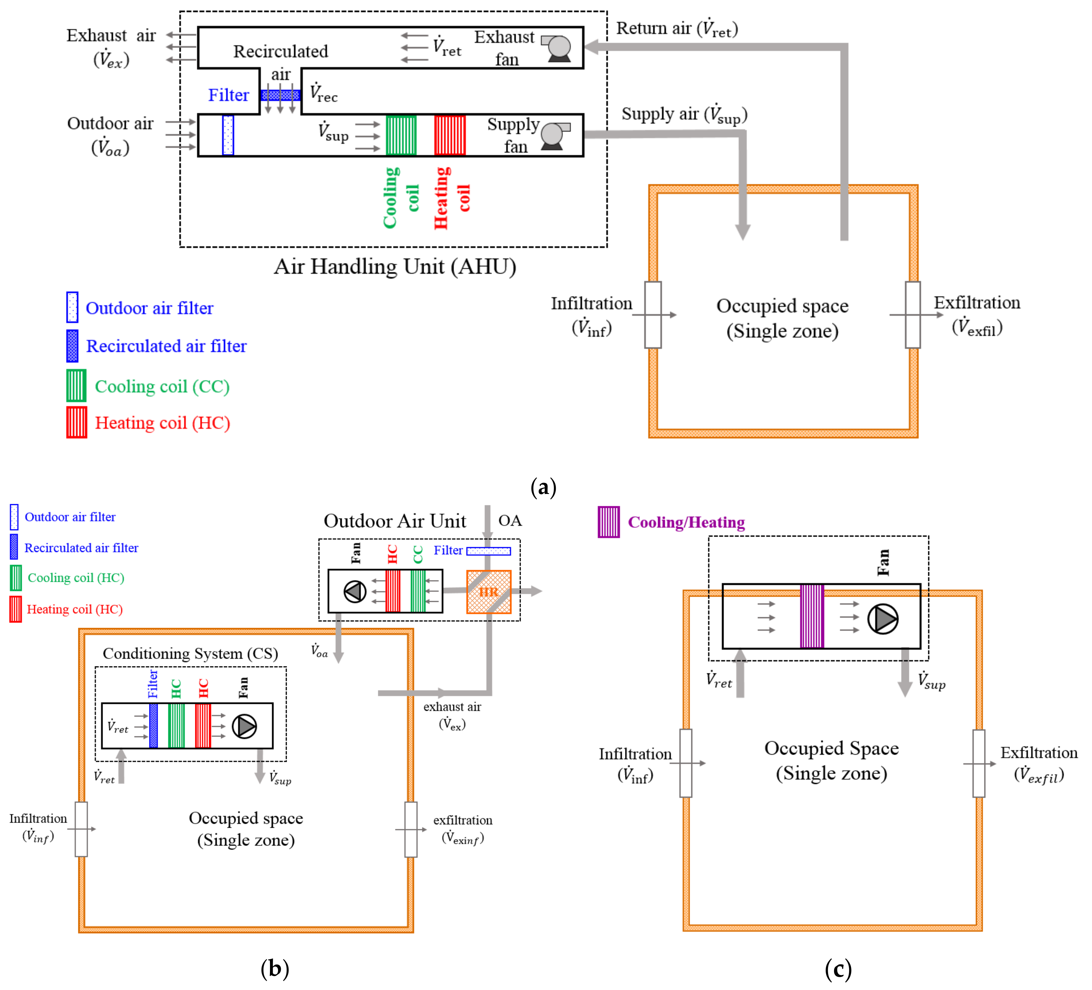
2. Description of HVAC Systems

This study focuses on a highly occupied indoor space, typical of the Spanish hospitality industry (e.g., bar and pub) with different HVAC system types. The HVAC systems considered are a central air handling system (CAHS), a dedicated outdoor air system (DOAS), and a wall unit system (WUS), which are applied to serve the occupied space as illustrated in Figure 2. The CAHS shown in Figure 2a can be placed on the rooftop or adjacent to the building. It is a constant air volume (CAV) system that supplies the space with a mix of outdoor air and recirculated air at the required supply airflow rate, while a portion of return air from indoors is exhausted out of the building. The DOAS depicted in Figure 2b uses a separate outdoor air unit (OAU) which supplies the required outdoor air directly to the indoor space after conditioning it to the indoor set point temperature. The air within the space is recirculated, filtered, and conditioned using a room-level air-conditioning system (CS in Figure 2b). The WUS considered in the study, illustrated in Figure 2c, is a through-the-wall room air conditioner, which does not supply outdoor air for ventilation or filter the return room air.
In the case of the CAHS shown in Figure 2a, a constant air volume (CAV) HVAC configuration is used to deliver the cooling and heating requirements of the conditioned space with a water-cooled electrical chiller and natural gas-fired boiler. The CHW loop design setpoint temperature and Δ T c h w are 8 °C and 6 °C, respectively, while the boiler HW loop design setpoint temperature and Δ T h w are 50 °C and 10 °C. The cooling water inlet temperature is set at 29.4 °C for the electrical chiller’s condenser that uses an evaporative cooling tower. The cooling coil and heating coil (which use chilled water and hot water, respectively) setpoint temperatures are 16 °C and 22 °C. In addition, the zone cooling and heating supply air temperatures are set to 16 °C and 35 °C, respectively. An air-to-air heat-recovery-type plate heat exchanger with sensible and latent heat recovery was considered. It should be noted that this simulation did not consider economizer, humidifier, dehumidifier, and coil preheat.
The DOAS, Figure 2b, consists of an OAU with an air-to-air heat recovery heat exchanger and a thermal conditioning system (CS) which recirculates, conditions, and filters the air in the indoor space. The DOAS is based on a four-pipe fan coil unit (FCU) connected to the chilled water and hot water loops of a central chiller plant and natural gas boiler (similar to the above CAHS). The supply fan total efficiency and motor efficiency were set to 70% and 90%. The V ˙ o a was set to 400 l/s on the basis of full occupancy and RITE’s standard (provided in Table 1). The performance of the electrical chiller and gas boiler was modelled using an average COP of 4.8 and a boiler efficiency of 92%, respectively. The FCU cooling and heating coils’ design setpoint temperatures were 24 °C and 20 °C, respectively. The recovery heat exchanger was modelled using a sensible and latent heat exchanger effectiveness of 70% and 65%, respectively.
The WUS, Figure 2c, was assumed to be an in-room air conditioner using a single-speed direct expansion (DX) cooling/heating coil with design cooling supply air ΔT of 8 °C and a heating design supply air temperature of 50 °C. A typical cooling COP of about 3.0 was considered for the DX system (coil) in this study. There is no mechanical OA supplied to the space, so the corresponding cooling (or heating) demand was not estimated.
As an example of a highly occupied indoor space, a representative bar/pub in Tarragona (Spain) was selected. It was served by three types of HVAC system, and its dimensions are given in Table 1. The bar/pub is part of a bigger building which is, at the same time, a hotel. Figure 3 illustrations a 3D view of the supposed representative single-zone room considered in the simulation. The main façade faces north. The bar/pub also has a door (2 m × 2 m facing south on the front wall) and two windows facing east on the left side of the building. As the hotel is a conditioned space at similar temperature as the bar/pub, it is also assumed that the floor, ceiling, and right and back walls of the room are adiabatic. The thermal transmittance, U, of the components of the building envelope are set to the limit values of thermal transmittance allowed for the January climate zone of Tarragona (Spain) according to the Technical Building Code of Spain. The details of U values and other input parameters are listed in Table 1.

3. Modelling Methodology

3.1. Modelling of Exposure to Virus-Laden Bioaerosols in an Indoor Space

In order to predict the transport and fate of an aerosolized virus within an indoor space, a simulation tool newly developed by the National Institute of Standards and Technology (NIST) of the United States, known as FaTIMA (Fate and Transport of Indoor Microbiological Aerosols), was used in this study [39,40,41]. This tool is based on a dynamic model of a single-zone room served by a mechanical ventilation system and uses mass conservation in the room to relate the aerosol sources. It also includes various removal mechanisms such as recirculated air filters, an in-room air cleaner, and a local exhaust fan besides removal due to natural processes like deposition (on surfaces) and decay. The aerosol concentration throughout the zone is uniform (i.e., a well-mixed approximation) [42,43]. However, more detailed methods can be used to study the influence of spatial variations on aerosols by using CFD simulations (e.g., in Refs. [44,45]). In this case, the governing mass balance for a single-zone volume of a room becomes [40]:
V z d C z d t = f p V ˙ i n f C o a t + V ˙ s u p C s u p t + G ˙ t V ˙ r e t + V ˙ l x + η a c V ˙ a c C z t k d , t o t
where C is the aerosol concentration in air (kg/m3), f p is the aerosol penetration factor (0 ≤ f p ≤1) from outside air into the room, G ˙ is the aerosol generation rate within the zone (kg/s), k d , t o t is the total aerosol deposition on surfaces (kg/s), V is zone volume (m3), V ˙ is the volumetric airflow rate (m3/s), t is time (s), and η a c is the in-room air cleaner (i.e., PAC) aerosol filtration efficiency (-).
The total surface area of deposited aerosols is estimated using:
k d , t o t = i = 1 n s u d , i A s , i C z t
where A s , i is the deposition area for surface i (m2), n s is the number of surfaces in the zone (floor, walls, ceiling, and others, if any), and u d , i is the aerosol deposition velocity for surface i (m/s). (Subscripts: ac = air cleaner in room, d = deposition, inf = infiltration, lx = local exhaust, oa = outdoor air, ret = return, sup = supply, tot = total and, z = zone.)
The surface loading for each surface, L s , i (kg/m2), is related to the deposition rate using Equations (3) and (4).
A s , i d L s , i d t = u d , i A s , i C z t
u d = k d V A s
where k d is the aerosol deposition rate (1/s).
According to Equation (1), the rate of change in mass of aerosols within the zone’s air volume is related to the aerosol source (i.e., outdoor air by infiltration V ˙ i n f , supply airflow V ˙ s u p , and aerosol generation within the zone G ˙ ) and the removal rate from the zone (the return airflow V ˙ r e t , the local exhaust airflow V ˙ l x , the air cleaner in the room η a c V ˙ a c , and the deposition on surfaces). The initial virus-laden aerosol concentration in both outside and indoor air is considered to be zero (i.e., C o a = 0.0 ) as only the effect of a contagious occupant sharing indoor space with other uninfected occupants is analyzed in this study.
The simulation tool model is based on CONTAM, which is a multi-zone indoor air quality and ventilation system computer program developed by NIST [46]. CONTAM computes on mass-based units [39,40] and inputs aerosol sources on a number basis (#), instead of a mass basis, since it converts mass into number-based variables using the specified aerosol diameter and density. Therefore, we analyze aerosols of a single size with an average aerodynamic diameter of 1 μm and a density of 1000 kg/m3 (approximated by using water density because of the aqueous properties of exhaled respiratory aerosols). The influence of relative humidity and temperature on airborne aerosol transmission is not taken into consideration. All airflow rate calculations are performed on a mass basis since the effect of temperature and pressure on the density of air is neglected and takes the density of air at 20 °C and 101.325 kPa (i.e., 1.2041 kg/m3).
The simulation outputs are obtained in terms of the time history of the aerosol concentration, the surface loading, and the integrated exposure that an occupant experiences in the zone [39,40]. The simulation period is set to be carried out for 24 h with a time step of 15 s. The integrated exposure, IE (kg·s/m3) given by Equation (5), is the integral of the aerosol concentration in air of the space/room in which the occupant is exposed during the exposure duration, indicated by the specific start and end time (i.e., t s t a r t and t e n d , respectively) [40].
I E = t s t a r t t e n d C z t d t
However, the occupant inhalation or body uptake rates, and the aerosol removal rate due to the presence of an occupant in the room, are not accounted for in this parameter. The IE, Equation (5), is used to analyze the effect of control measures on the relative reduction of virus-laden aerosol exposure of occupants under several scenarios. The normalized integrated exposure (NIE) is used to evaluate the relative reduction in virus-laden aerosol exposure caused by the control measures. Hence, NIE for a given HVAC system, N I E HVAC , is defined as the ratio of IE with and without control measures as given by Ng et al. [47]:
N I E HVAC = 1 η m a s k × I E HVAC , c o n t r o l I E HVAC , n o c o n t r o l
where η m a s k is the aerosol filtering efficiency (i.e., protection efficiency) of the mask worn by an exposed occupant, and the HVAC system can be CAHS, DOAS, or WUS.
The equivalent clean ACH (air changes per hour), E C A C H z given by Equation (7), is used to denote the “clean” airflow provided to the single-zone room as a combination of outdoor air supplied by the mechanical ventilation system ( ACH o a ), outdoor air delivered via infiltration ( ACH i n f ), and the control measure ( E A C H c o n t r o l ). The control measure can be a single measure or a combination of measures applied to provide the equivalent clean air (i.e., C = 0 ) to the zone, which can be HVAC and/or non-HVAC controls. The E A C H c o n t r o l consists of enhanced filtration in the recirculated air using HVAC filters based on MERV rating, the addition of a PAC, or the use of a local exhaust fan. Aerosol deposition on interior surfaces is not taken into account in the E C A C H z . The estimated relative reduction in virus-laden bioaerosols exposure, in terms of N I E HVAC obtained by using Equation (6), correspond to the equivalent clean ACH (and its value is calculated using Equation (7)) delivered by the applied control measures.
E C A C H z = ACH o a +   ACH i n f + E A C H c o n t r o l
The outdoor air flowrate, V ˙ o a , is the minimum requirement defined by the RITE. This depends on the building’s use, which, in turn, defines the indoor air quality category and the minimum requirement of outdoor air per person (or floor area) [36]. Then, the ACH o a is calculated as the ratio of V ˙ o a (in l/s) and zone volume ( V z in m3):
ACH o a = 3.6 V ˙ o a V z = 3.6 R p N z V z
where R p is the outdoor air flowrate (l/s/person), and N z is the number of occupants in the zone (full occupancy), which may be obtained from the default occupancy based on the ASHRAE standard 62.192019 or local regulations for a specified space type [37]. The outdoor air infiltration rate,   V ˙ i n f , through the building’s envelope is obtained using a typical value for ACH i n f , although infiltration is dependent on several factors (for instance, wind speed and direction, indoor/outdoor temperature difference, and HVAC system operation [48]) and is outside the scope of this study.
The supply airflow rate, V ˙ s u p , is determined from the peak cooling/heating loads estimated in the design conditions set for the highly occupied indoor space, which is modelled and simulated with the EnergyPlusTM simulation program [49]. Then, the outdoor air intake fraction, f o a , of the ventilation system is calculated as the ratio of supply and outdoor air flow rates (i.e., f o a = V ˙ o a / V ˙ s u p , f o a 1.0 ). The total outdoor air ACH, ACH o a , t o t , can be calculated using [40]:
ACH o a , t o t = V ˙ o a + V ˙ i n f m i n   0.0 , V ˙ b a l V z
where the balance airflow rate of the zone is given by Equation (10).
V ˙ b a l = V ˙ s u p + V ˙ i n f V ˙ r e t V ˙ l x
The recirculation airflow rate, V ˙ r e c , which is the amount of return air, if any, recirculated back to the zone by the air handling system is calculated as:
V ˙ r e c = m i n V ˙ r e t , V ˙ s u p 1 f o a
According to recent guidelines for HVAC system operation in buildings during the COVID-19 pandemic, air should not be recirculated if at all possible [28]. If recirculation cannot be avoided, the recirculated air should be filtered before being mixed with the fresh outdoor air intake in the AHU. Thereby, different air filters, rated by MERV 4–16, are implemented in the FaTIMA model using the efficiency prediction model developed by Kowalski et al. [50]. However, even though it is validated with experimental data, there are some discrepancies between this filter efficiency model and the minimum requirements available in ASHRAE 52.2-2017 for the MERV rating [47]. Therefore, the overall/equivalent clean ACH due to filtration of the recirculated air is:
ACH r e c = η f i l t e r V ˙ r e c V z
where η f i l t e r is the filter efficiency, which depends on the aerosol/particle size. Since the virus-laden aerosol concentration in the outdoor air is assumed to be zero, an outdoor air filter is not used in this study.
The clean ACH delivered by the air cleaner in a room, ACH a c , is calculated as:
ACH a c = η a c V ˙ a c V z = η a c f a c   V ˙ a c , m a x V z
where η a c is the aerosol filtering efficiency of the air cleaner obtained from the MERV rating charts for an aerosol diameter of 1 μm. V ˙ a c and   V ˙ a c , m a x are the actual fan airflow rate and the maximum fan airflow rate, respectively, of the air cleaner, and f a c is the fraction of fan flow rates (i.e., f a c = V ˙ a c / V ˙ a c , m a x and 0 f a c 1 ), which makes it possible to use air cleaners with multiple airflow rate settings. Therefore, the clean air delivery rate, CADR , of the air cleaner, is calculated as:
CADR = η a c   f a c   V ˙ a c , m a x
The removal of aerosols from the room air because of deposition on surfaces (i.e., floor, walls, ceilings, and others) is estimated by using the effective deposition rate, k e f f , defined as:
k e f f = u d , f   A f + u d , w   A w + u d , c   A c + u d , o A o   V
where u d , f , u d , w , u d , c , and u d , o are the deposition velocity for floor ( 3.4 × 10 5 m/s), walls ( 1.13 × 10 5 m/s), ceiling ( 1.75 × 10 6 m/s), and other (0.00 m/s) surfaces. The aerosol deposition velocity is a function of friction velocity ( u * ), and this study takes a conservative value on the basis of the highest reported value (i.e., u * = 1.0 m/s) by Dols et al. [40]. The value of k e f f determined by using Equation (15) does not include the aerosol deactivation rate. Since viruses may lose viability to cause infection during the airborne phase, the simulation model includes the biological decay rate of SARS-CoV-2 ( λ d e c a y in h−1) estimated by using Equation (16) and a half-life ( τ 1 / 2 ) of 1.1 h [16,51].
λ d e c a y = ln 0.5   τ 1 / 2

3.2. Estimation of the Energy Consumption of the Control Measures

This subsection describes the methods used to estimate the annual energy consumption of each control measure, that is to say, mechanical ventilation using OA with several values of f o a ( 0.0 f o a 1.0 ), recirculated air filtration with MERV rating (≥MERV 13), PACs, and local exhaust fans.
The energy consumption of ventilation using OA depends on whether it has to be cooled or heated to bring it to the desired level of comfort (i.e., temperature and relative humidity) and, therefore, is highly dependent on climate conditions (e.g., [52,53]). The influence of daily variation can be reduced by using an economizer, which automatically increases ventilation rates when the outdoor air conditions are favorable from an energy consumption viewpoint. However, such control strategies (e.g., free cooling at night) are not commonly implemented in existing buildings. Moreover, heat-recovery technologies can be implemented to minimize the energy impact of ventilation.
In this study, the energy consumption associated with ventilation and other heating/cooling loads in the indoor space is simulated using the EnergyPlusTM software, v9.3.0 [49], which provides a reliable estimate of the building’s energy consumption based on the weather conditions of the location and the building use.
The amount of energy required to sustain the desired indoor conditions is associated with the cooling or heating demand of the indoor space. The cooling/heating demand is estimated by considering the gains and losses in building heat such as heat transmission via building envelope elements, infiltration air heat gains/losses, fresh OA ventilation heat gains/losses, and internal heat gains from occupants, solar radiation, artificial lighting, and electrical equipment. The thermal characteristics of the building envelope are regulated in Spain by the requirements of the Technical Building Code (CTE-DB-HE), which must be obeyed by both new and renovated buildings. The CTE-DB-HE has recently been modified to comply with the requirements for achieving nearly zero-energy buildings (NZEBs) [29]. The U-values of building elements (i.e., exterior wall, ground floor, flat roof, windows, and door) were chosen based on the limit values established by the current (after 2020) [29] and previous CTE-DB-HE (2006–2019) [30,31,34].
As far as the auxiliary components of the CAV HVAC system are concerned, the supply (and return) fan and motors were modelled using their typical efficiency values (i.e., 70% total fan efficiency and 90% electrical efficiency). The supply fan total efficiency and motor efficiency of the DOAS were also set to 70% and 90%.
The implementation of an HVAC filter in the recirculated air duct needs additional fan power because of the pressure drops raised due to the particulate filtration. The additional annual electrical energy consumption, E f i l t e r in kWhel, can be reasonably estimated by considering the pressure drop of the recirculated airflow across the filter using [54,55]:
E f i l t e r = V ˙ r e c   Δ P ¯ f i l t e r × 10 6 ƞ f a n   ƞ m   t o p t
where Δ P ¯ f i l t e r is the average pressure drop across the HVAC filter in Pa, ƞ f a n and ƞ m are the total mechanical efficiency (70%) and electric motor efficiency (65%), respectively, of the variable speed fan, and t o p t (in h) is the annual fan operational time. The fan was assumed to operate for an hour before the building was occupied and then operated throughout the period it was occupied.
For an in-room air cleaner (i.e., PAC), the electrical energy consumption ( E P A C in kWh/year) can be estimated from the device’s rated power using Equation (18). Theoretical models can also be found in the literature for estimating and optimizing the overall particle removal rate for a given level of electricity consumption [56]. However, it is advisable to use power consumption data obtained from the device’s manufacturer specifications at the maximum fan speed (and other fan speeds, i.e., flow rates, when variable speed operation devices are used) [43]. The PAC energy efficiency must be determined with a standard test, and it is defined as a clean airflow rate per unit of electrical power consumed (e.g., it will be assigned to one of the classes of Eurovent Certita Certification for Clean Air Efficiency, that is to say, between A-class (>13 m3/h/W) and E-class (<2 m3/h/W)) [57,58]. According to a recent online survey on commercial PAC, the average electrical power consumed per CADR is about 0.15 W/(m3/h) [59].
E a c = S E C a c CADR a c t o p t = S E C a c η a c f a c V ˙ a c , m a x   t o p t
where S E C P A C is the PAC specific energy consumption in W/(m3/h) and CADR P A C the clean air delivery rate in m3/h of the air cleaner.
The electricity consumption of a local exhaust fan, E f a n , l x in kWh, can be estimated using the rated power of the fan motor indicated on its nameplate. Even though the amount of electricity consumed can be estimated more accurately when models calibrated using actual operating data are used, the nameplate power rating and design airflow rate of the fan also provide a reasonable estimation for this type of energy analysis.

4. Results and Discussion

Section 4.1, Section 4.2, Section 4.3 present and discuss the simulation results obtained regarding the effect of HVAC and non-HVAC control on the reduction of exposure to virus-laden bioaerosols of uninfected occupants in a highly occupied indoor space (i.e., a typical bar or pub in Tarragona, Spain). The level of bioaerosol exposure on uninfected occupants sharing the same indoor space with an infected individual is investigated first in Section 4.1 in baseline conditions (Table 2) and with the other input modeling parameters listed in Table 1. Then, the effect of the control measures listed in Table 2 on the reduction of infections resulting from aerosol exposure is analyzed in an individual (Section 4.2) and combined form of implementation (Section 4.3). The energy consumption associated with each control measure is estimated and discussed.
The susceptibility of individuals exposed in indoor spaces to the presence of an asymptomatic or pre-symptomatic subject infected with SARS-CoV-2 has been examined in recent studies (e.g., [15,16,44]). The aerosol generation rate, G ˙ , of an infected occupant was set to 686 #/min by considering the average adult exhalation rate and the number of exhaled aerosols (in through the nose and out through the mouth). The exhaled aerosols number is determined based on experiments carried out on healthy individuals (i.e., 98 #/min) [60]. This value does not assume that all the aerosols contain viruses or define a specific concentration of aerosol in occupied indoor space that is sufficient to cause COVID-19 [47]. In order to analyze the impact of each control measure, in this study, results are given in terms of relative reduction in infectious human aerosol exposure, so the main results are normalized values. Hence, the absolute value of the aerosol generation rate has little impact on the outcome of a study of this type and an arbitrary G ˙ can also be used (e.g., 500 #/min used by Ng et al. [47]). Additionally, although the model can accommodate intermittent aerosol generation sources like coughing, such sources are not considered in this analysis within the occupancy duration (i.e., 3 h per day, 20:00–23:00).
The supply airflow predicted by the EnergyPlus simulation, V ˙ s u p , from the internal and external heat gains of the fully occupied room (listed in Table 1) was about 620 l/s for the CAHS, 618 l/s for the DOAS, and 627 l/s for the WUS. According to Spain’s CTE, the influence of the building’s envelope Ulimit, on the calculated V ˙ s u p was minor due to the high internal heat gains in the space (e.g., the CAHS V ˙ s u p increased by <1.0%, from 620 l/s to 625 l/s, when the Ulimit was based on the CTE until 2019 instead of CTE-DB-HE1 2019). The simulated building data was obtained using typical meteorological year (TMY3) data from Tarragona (Spain).
The main drawback of the DOAS is that it is designed for a specific mechanical ventilation rate (e.g., 400 l/s in this case) and cannot readily accommodate considerably increased ventilation rates, while the WUS has no mechanical ventilation with outdoor air. Therefore, the increase in OAF was only applicable in the case of CAHS from about 0.65 up to one (i.e., V ˙ o a = 620 l/s). It is also assumed that the HVAC systems (i.e., CAHS, DOAS, and WUS) began to operate an hour before the building was occupied.
Figure 4 shows the simulated thermal load (heating and cooling loads) and temperature profile (outdoor and indoor air) for the design days in summer and winter conditions and for the three HVAC systems studied. As the conditioned zone is highly occupied, the thermal loads are especially affected by occupancy density (i.e., of 100 #/100 m2), resulting in a much higher requirement for cooling than heating. In this respect, heating requirements are mostly required on cold days to heat the outdoor airflow into the space.
In summer, the three HVAC systems have similar cooling requirements and profiles. However, in winter, their thermal loads and profiles are very different. In this regard, after the bar had been heated for the first hour after opening with CAHS, heating was still required during the following hours as the heating requirements of the outside air flow rate were higher than the internal cooling loads. On the other hand, the DOAS and the WUS were only required for heating during the first hour of opening, and, after that, cooling was required. For the WUS, no heating was required as no outside air was supplied. For the DOAS, no heating was required because the outside airflow did not need to be heated up as much as for the CAHS. Moreover, for the DOAS, the outside airflow rate decreased the cooling required in comparison with WUS.

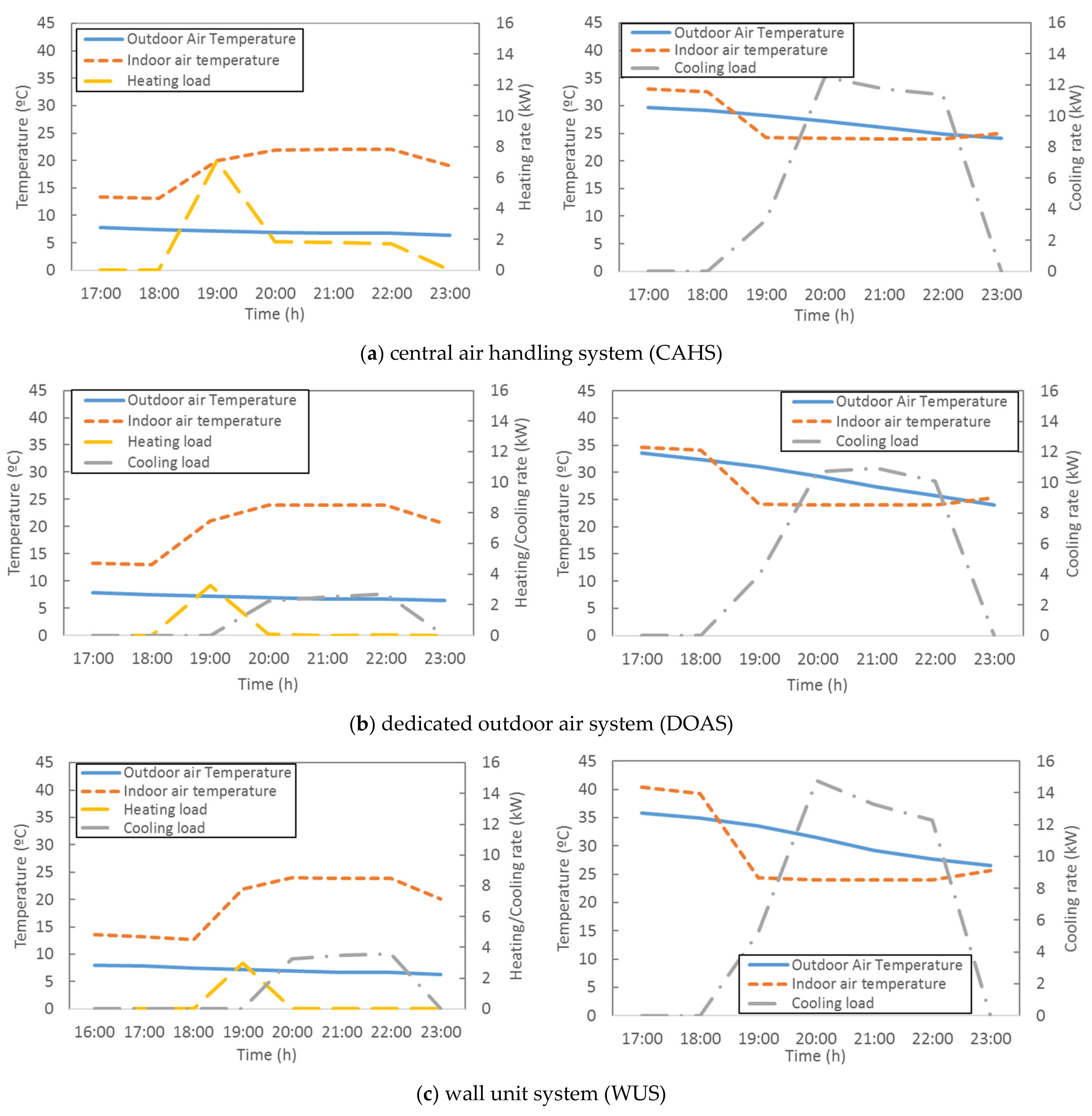
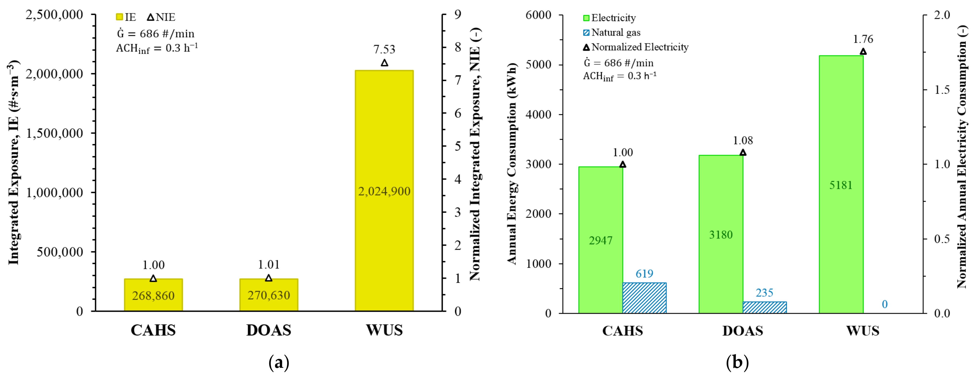
4.1. Baseline Analysis

The design supply airflow rate of each HVAC type (i.e., CAHS, DOAS, and WUS) was based on the peak cooling loads. Table 3 shows the peak cooling and heating loads, and the annual thermal demands (i.e., cooling and heating) of the simulated indoor space under full occupancy (i.e., 50 individuals).
Figure 5a shows the normalized and integrated exposure (NIE and IE) of the bar/pub with a simulated volume of 150 m3 for each type of HVAC system (Figure 2) based on the base-case conditions listed in Table 2. The exposure to aerosols of the room occupants, evaluated using IE and NIE, was estimated for 3 h/day of continuous exposure to a continuous bioaerosols source for the same duration. The NIE values reported in Figure 5a were obtained by normalizing the IE associated with each HVAC system type by using the lowest IE (which was for the CAHS).
The base-case IE value of the WUS was over seven times higher than of the CAHS and DOAS, largely because OA was not supplied by the WUS ventilation system but was by CAHS and DOAS. The ACH of OA in the CAHS and DOAS were 9.97 h−1 and 9.90 h−1, respectively, while for the WUS, it was only 0.3 h−1 (due to ACH of OA delivered by the infiltration). Therefore, the type of HVAC system clearly has an impact on the IE value, especially in the case of WUS (i.e., 2,024,900#·s/m3), which has no mechanical OA supply system.
The IE reported in Figure 5a does not include the decay rate of the virus in aerosols ( ~ 0.63 h−1) and the aerosols deposited on surfaces ( ~ 0.067 h−1). The surface loading is detailed in Appendix A. In addition, the transient aerosol airborne concentration and the exposure within 24 h are shown in Appendix B.
The associated annual energy consumption (i.e., electricity and natural gas) of the three HVAC systems is shown in Figure 5b. This figure is the energy required by the HVAC system including the power required by the chiller and the auxiliaries and the natural gas required by the boiler. Finally, the heating and cooling required are provided by the cooling and heating coils described in Section 2.

4.2. Effect of Individual Control Measures

This section analyzes the effect of the control measures listed in Table 2 on the reduction of virus-laden aerosol exposure of uninfected occupants sharing the same indoor space with a COVID-19-infected individual (asymptomatic or pre-symptomatic).
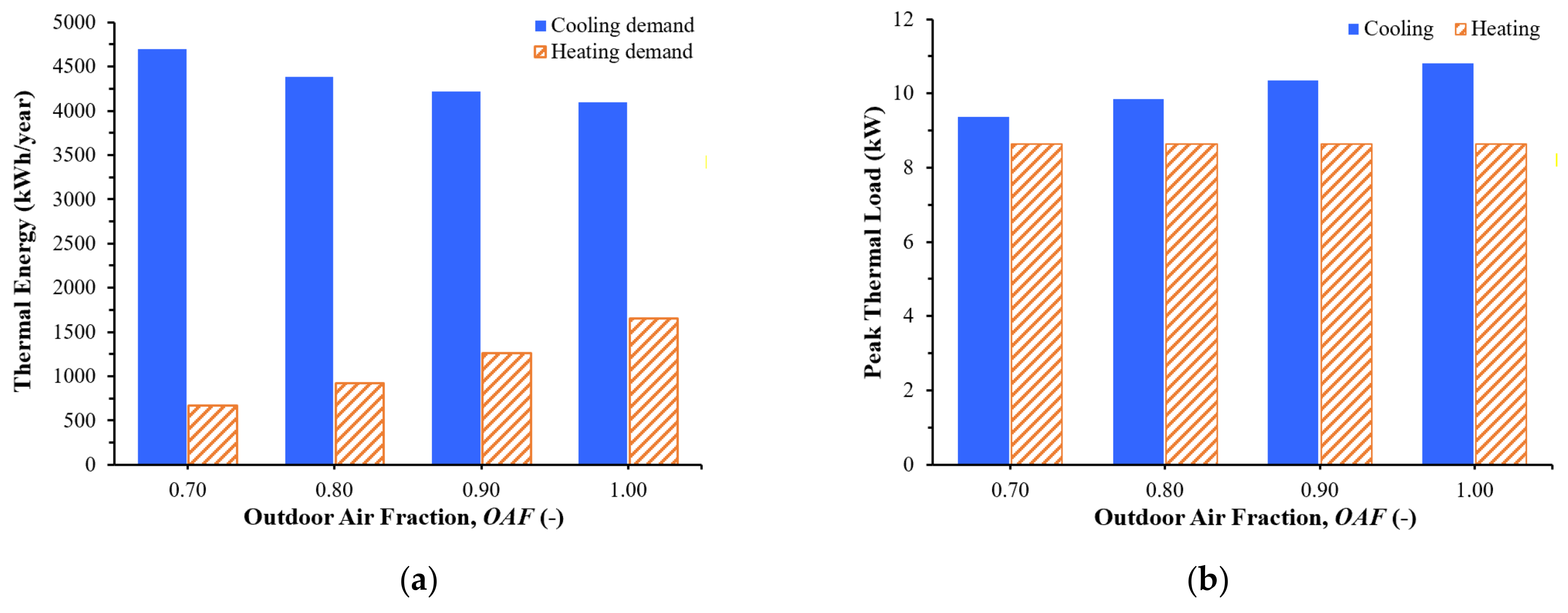
  • Effect of the outdoor air fraction (OAF): Figure 6a shows the effect of increased mechanical ventilation using OA on the NIE for the CAHS versus OAF. The associated annual energy consumption (i.e., consumed electricity and natural gas) of this enhanced mechanical ventilation mitigation strategy, for several OAF values, is illustrated in Figure 6b. The equivalent clean ACH increased from 9.9 h−1 to 15.2 h−1 when the OAF was increased from ~ 0.65 to 1.00, at an outdoor airflow rate ranging from 400 l/s to 620 l/s. The OA ventilation rate per person increased from about 8.0 l/s/person to 12.4 l/s/person in the same range of OAF. The annual consumed electricity dropped by about 8.9% when the outdoor airflow rate was increased from the base case (i.e., 400 l/s) to 620 l/s, while natural gas consumption increased by more than twofold in the same range (Figure 6b). This is due to the 16.3% drop in annual cooling demand and the almost 1.9-fold rise in annual heating demand when the outdoor airflow rate increased from 400 l/s to 620 l/s (Figure 7). The peak cooling and heating demand of the fully occupied indoor space is also shown in Figure 7 at the different outdoor airflow rates (i.e., OAF) considered in this study.
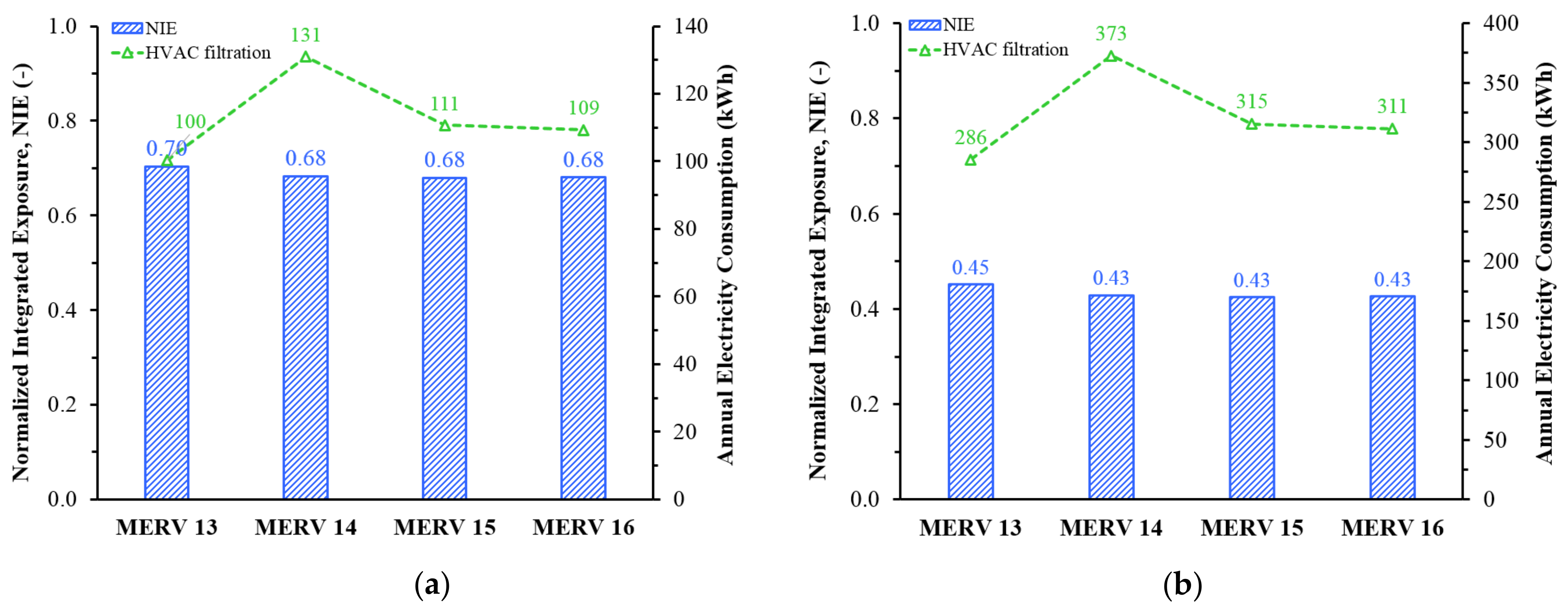
  • Effect of recirculated air filtration: Figure 8a,b show the influence on the NIE of recirculated air filtered with HVAC filters with MERV ratings between MERV 13 and MERV 16 for the CAHS (Figure 2a) and DOAS (Figure 2b), respectively. The additional electricity consumed for recirculated air filtration (see Figure 8a,b) is estimated from the power consumption of the fan required to overcome the pressure drop caused by the HVAC filter, and the fan operational time (i.e., 4.0 h per day for 365 days per annum). The average pressure drops of the MERV-rated HVAC filters, reported in Azimi and Stephens [54], were used to estimate the power consumption of the fan. Since there is no HVAC filter for the return air stream of the WUS (Figure 2c), the influence of return/recirculated air filtration was not analyzed. In both CAHS and DOAS, the calculated NIE values were almost the same (0.68−0.70 and 0.43−0.45, respectively) when HVAC filters with MERV 13 and higher ratings were implemented for the aerosol size considered (i.e., a diameter of 1.0 μm). In addition, the NIE decreased more in the DOAS than in the CAHS as the recirculated airflow was higher. The equivalent clean ACH increased from 14.66 to 15.13 h−1 for the CAHS and 23.25 to 24.58 h−1 for the DOAS when the HVAC filter efficiency rating was raised from MERV 13 to MERV 16. In the CASH, the increase in electricity consumption when there were filters in the recirculation flow ranged from 3.4% to 4.5%, whereas in the DOAS it ranged from 9.0% to 11.7%.
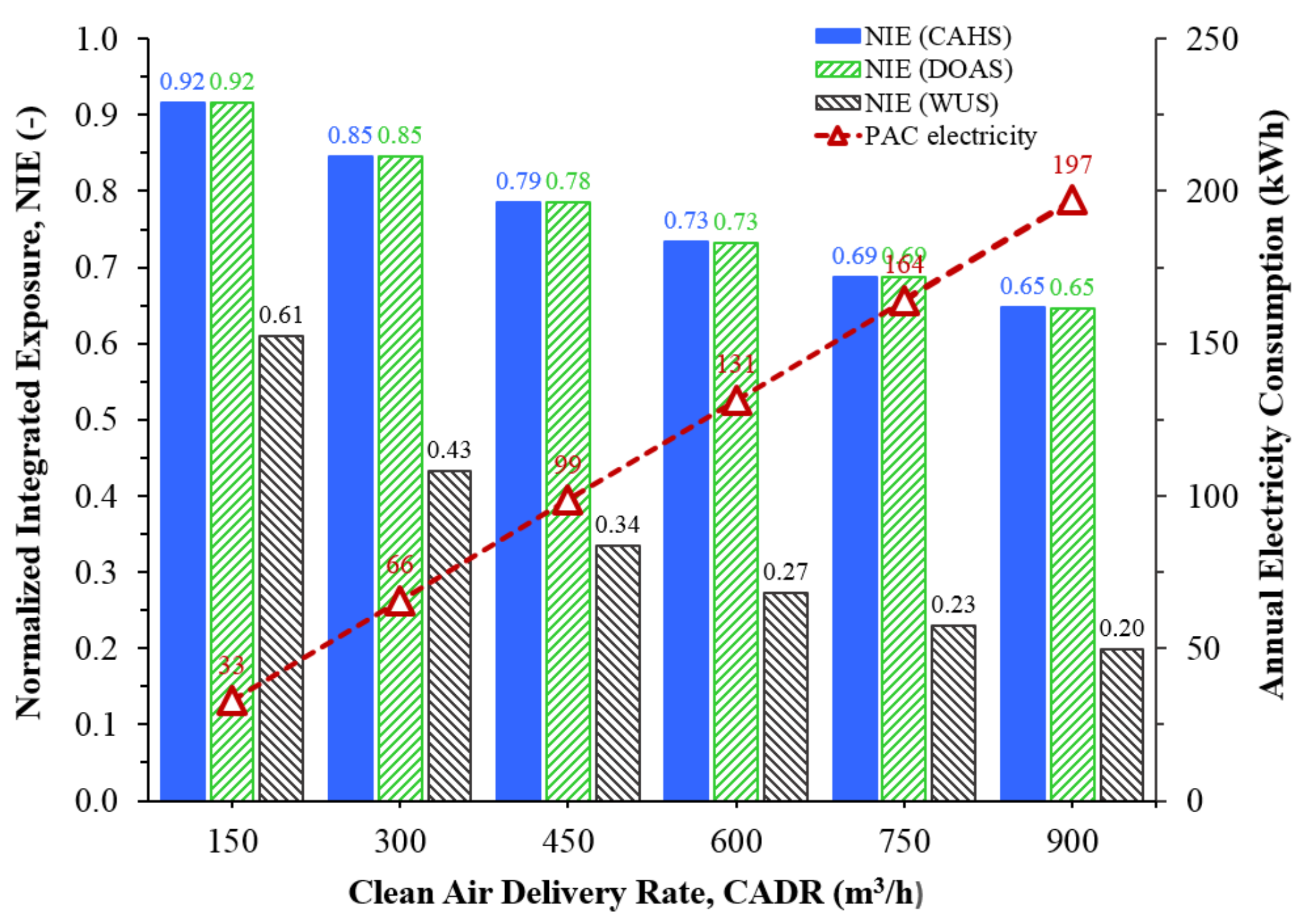
  • Portable air cleaner (PAC): The use of a PAC to reduce the virus-laden bioaerosol exposure of building occupants is an advantage when extra ventilation using outdoor air and/or recirculated air filtration is not possible, as in the case of WUS. Hence, the effect of PAC on the reduction of aerosol exposure was simulated with each type of HVAC system (i.e., CAHS, DOAS, and WUS, as shown in Figure 2) serving the indoor space. The effect of the PAC on NIE was simulated using six different CADR values, which are specified in Table 2 in terms of EACHpac (i.e., 1.0–6.0 h−1). For the three HVAC types, Figure 9 compares the influence of PAC on the reduction of aerosol exposure to the base-case in terms of NIE. When the EACHpac was increased from 1.0 h−1 to 6 h−1, the maximum airflow rate via the PAC was approximately 42 l/s to 253 l/s with a filtering efficiency of 99% for an aerosol diameter of 1.0 μm. The electricity consumed by the PAC to deliver the clean ACH is also depicted in Figure 9. The influence of the PAC CADR on the NIE is similar in the CASH and DOAS (it decreases in both from 0.92, when the CADR is 150 m3/h, to 0.65, when the CADR is 900 m3/h), and much higher in the WUS (it decreases from 0.61, when the CADR is 150 m3/h, to 0.20, when the CADR is 900 m3/h). The increase in energy consumption with the PAC unit is small, always below 200 kWh/year.
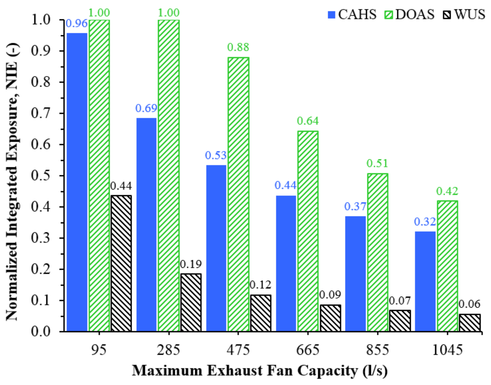
  • Exhaust fan: The commercially available box fans can be installed in a room (e.g., in windows or doorways) to exhaust contaminated air out of the indoor space, thus reducing the exposure of occupants to infectious bioaerosols. The effect of the exhaust fan on NIE, which was simulated with different capacities (maximum airflow rates, Table 2), is shown in Figure 10. Electricity consumed by the exhaust fans can be estimated as it was for the PAC (Figure 9) by using the operating hours and rated power of the box fan, indicated on its nameplate, existing in the market.

4.3. Effect of Combined Control Measures

Figure 11a illustrates the combined effect of control measures on the reduction of virus-laden aerosol exposure to uninfected occupants for each type of HVAC system. These control measures include mechanical ventilation using OA based on the RITE standard (i.e., an OA air supply of 8 l/s/person), enhanced recirculated air filtration using a MERV 13 filter in the CAHS and DOAS (90% efficiency for considered aerosol diameter of 1.0 μm), and PACs of several capacities (i.e., 150–900 m3/h of CADR). The annual electricity consumption of these control measures (Figure 11a) is depicted in Figure 11b. The NIE values and normalized electricity consumption reported in Figure 11a,b, respectively, were obtained by normalizing the corresponding IE and annual electricity consumption of each combined control measure with the base-case values.
As well as consuming electricity, CAHS and DOAS also consume 619.44 kWh/year and 234.67 kWh/year of natural gas, respectively, to supply the heating requirement of the conditioned indoor space.
The operational costs of the control measures can be estimated from the electricity and natural gas consumption reported in the present study and the current electricity and natural gas prices. The cost of electricity to run PACs is cheaper than other control measures, such as ventilation using outdoor air if the required aerosol mitigation is reached by using the PAC. For instance, the average yearly cost of electricity to run a portable HEPA air cleaner all the time is between USD 100 and 250 [61]. Filter replacement costs should also be included in estimating the annual overall cost of the PACs.
Finally, it should be noted that other technologies such as the ultraviolet germicidal irradiation (UVGI) system and photocatalytic oxidation (PCO) for reducing aerosol transmission have not been included in this study, but they also have the potential to mitigate airborne virus propagation in indoor spaces. Nor does the modeling and simulation methodology include non-airborne routes of exposure (e.g., direct/indirect contact with fomites), so the control measures discussed should be implemented together with other strategies (e.g., hand washing).

5. Concluding Remarks

Three common types of HVAC system were analyzed for controlling the spread of virus-laden bioaerosols in a highly occupied indoor space (floor area of 50 m2 and an occupancy density of 100 #/100 m2) in Tarragona (Spain) weather conditions. The space was analyzed for 3 h/day of continuous exposure of occupants sharing the space with an infected subject. The HVAC system types were a central air handling system (CAHS), a dedicated outdoor air system (DOAS), and a wall unit system (WUS). The base-case occupant bioaerosol exposure for CAHS and DOAS was studied by considering the effect of mechanical ventilation with an outdoor airflow rate in compliance with the Spanish regulation (i.e., RITE standard, 8 l/s/person), whereas the WUS had no mechanical ventilation. The combined effect of mechanical ventilation (i.e., 400 l/s of outdoor air), recirculated air filtration using a MERV 13 that is 90% efficient (for an aerosol diameter of 1 μm), and a portable air cleaner (PAC) with a capacity in the range 150–900 m3/h of CADR mitigated the (normalized) integrated exposure of the occupant by ~ 0.66 to 0.51 and 0.43 to 0.36 for the CAHS and DOAS, respectively. In the case of WUS, the normalized integrated exposure was reduced by up to 0.2 when the PAC with a capacity of up to 900 m3/h was used. The electricity consumed by these combined control measures increased by approximately 297.37 kWh/year and 482.66 kWh/year for the CAHS and DOAS, respectively, in comparison to the base-case, while for the WUS, it increased by about 197.10 kWh/year.
Even though the simulated occupant exposure (in terms of IE and NIE) is not a direct measure of the infection risk of occupants sharing a space with an infected subject, it can be used to effectively identify the best strategies for reducing building occupant exposure to airborne pathogens. Therefore, estimating the energy consumed by the control measures is useful for selecting cost-effective control strategies for the different types of HVAC systems in buildings.
In conclusion, the methodology in this study helps to select the best control options for the type of HVAC system in a building and reduce energy consumption. Thereby, control solutions can be implemented economically, and the indoor air quality can be guaranteed to be sufficient for human health. Thereby, risks related to the airborne transmission of COVID-19 (and alike diseases) can be effectively mitigated in highly occupied indoor spaces in hotels including bars and pubs by applying cost-effective control measures. Thus, other imposed non-engineering control measures can be relaxed/removed (such as reduction in occupancy level) due to COVID-19 preventive measures so that indoor activities can be increased to their full capacity.

Author Contributions

D.S.A.: conceptualization, methodology, software, investigation, writing—original draft preparation, writing—review and editing; J.P.: conceptualization, methodology, software, investigation, writing—review and editing; F.R.: software, investigation; G.G.: conceptualization, investigation; J.A.D.: conceptualization, investigation; A.C.: supervision, resources, project administration, funding acquisition. All authors have read and agreed to the published version of the manuscript.

Funding

The research work presented in this paper is the outcome of a project funded by Diputació de Tarragona under the collaboration framework agreement between the Diputació de Tarragona and the Universitat Rovira i Virgili for the period 2020–2023 with the reference number 2020/19: reference number 2020/19.

Acknowledgments

John F. Bates, coordinator of the language service at the Universitat Rovira i Virgili, is acknowledged for his editing contribution to the final version of the manuscript.

Conflicts of Interest

The authors declare no conflict of interest.

Nomenclature

AHUair-handling unit
ASHRAEAmerican Society of Heating, Refrigerating, and Air-Conditioning Engineers
CAHScentral air handling system
CAVconstant air volume
CCcooling coil
CHWchilled water
COVID-19coronavirus disease 2019
DOASdedicated outdoor air system
DXdirect expansion
HCheating coil
HEPAhigh-efficiency particulate air
HRheat recovery
HVACheating, ventilation, and air conditioning
HWhot water
HXair-to-air heat recovery heat exchanger
MERVminimum efficiency reporting values
OAoutdoor air
PACportable air cleaner
RITESpanish thermal building regulations
SARS-CoV-2severe acute respiratory syndrome coronavirus 2
WUSwall unit system
Main Notations
Aarea (m2)
ACHair changes per hour (h−1)
C ˙ aerosol concentration in air (kg/m3)
CADRclean air delivery rate (m3/h)
COPcoefficient of performance (-)
Eelectrical energy (kWh)
ECACHequivalent clean air change rate (h−1)
ffraction (-)
G ˙ aerosol generation rate (kg/s or #/min)
INintegrated exposure (#·s/m3)
NINnormalized integrated exposure (-)
OAUoutdoor fraction (-)
Ppressure (kPa)
SECspecific energy consumption (W/(m3/h) or kW/(m3/h))
Ttemperature (°C)
Uthermal transmittance (W/m2 K)
uvelocity (m/s)
Vvolume (m3)
V ˙ volumetric airflow rate (l/s or m3/s)
Greek symbol
Δ difference
summation
ƞefficiency
λlamda
κkappa
Subscript
acair cleaner
chwchilled water
ddeposition
exexhaust
effeffective
exfilexfiltration
hwhot water
infinfiltration
lxlocal exhaust
oaoutdoor air
recrecirculated
retreturn
supsupply
tottotal
zzone

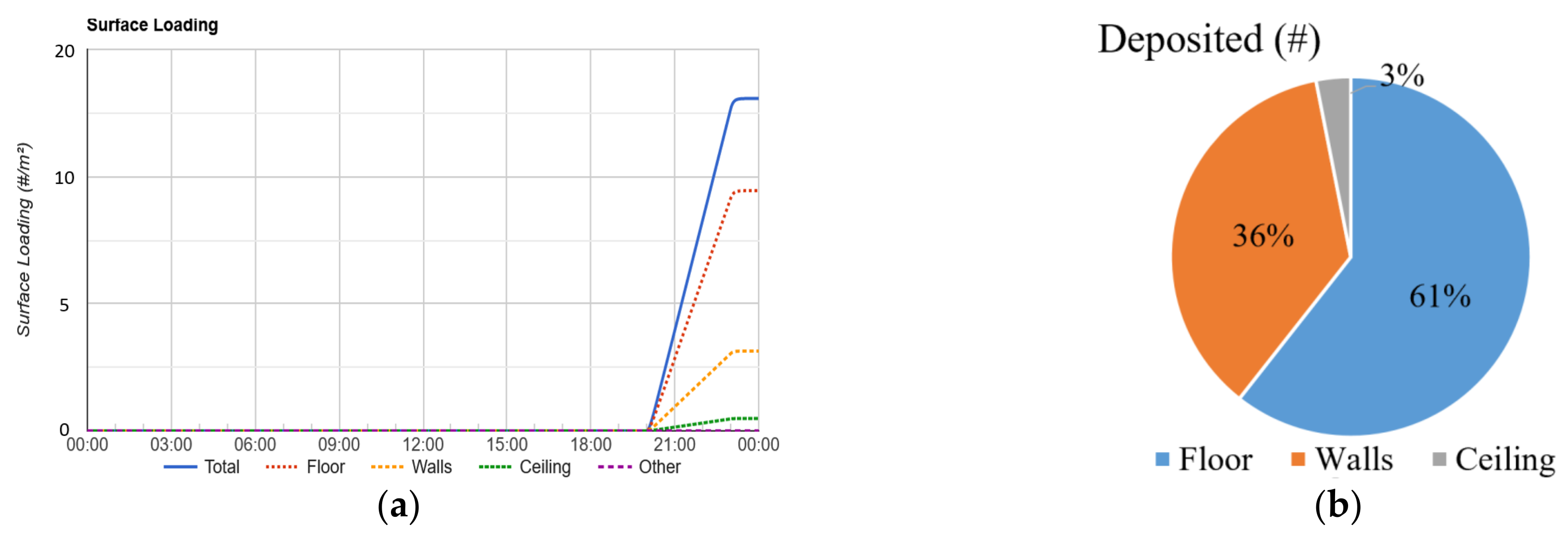
Appendix A. Aerosol Deposition on Surfaces

Figure A1. Aerosols deposited on the surfaces of the indoor space: (a) transient surface loading; (b) percentage of aerosols deposited on each surface.
Energies 15 00937 g0a1

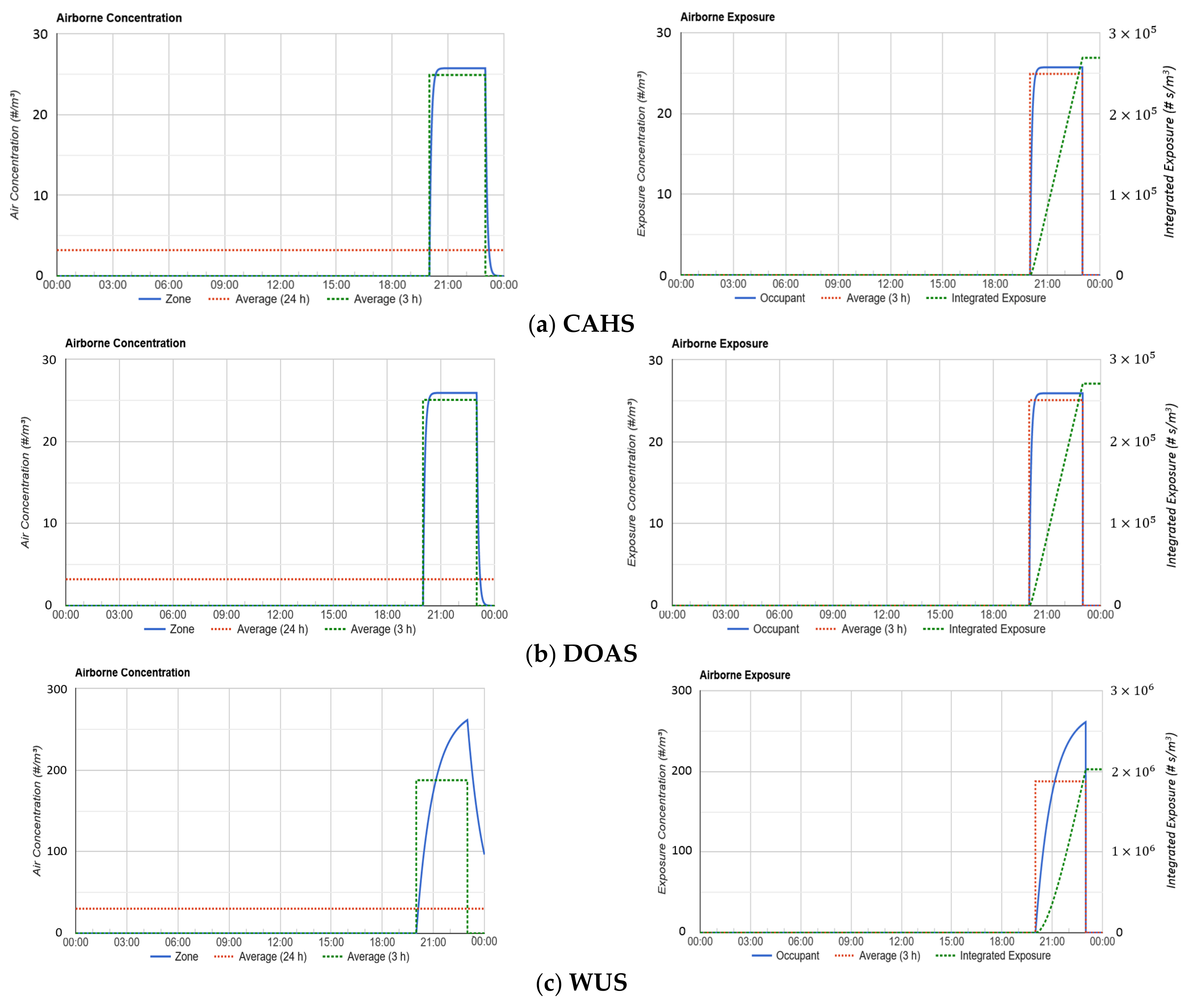
Appendix B. Aerosol Airborne Concentration and Exposure within the 24 h

Figure A2. Transient aerosol airborne concentration and exposure within the 24 h for a highly occupied indoor space served by three different HVAC systems.
Energies 15 00937 g0a2

References

  1. Instituto Nacional de Estadística (INE). Spanish Tourism Satellite. Statistical Review 2019; 2016–2019 Series; Press Releases: Madrid, Spain, 2020; p. 4. [Google Scholar]
  2. Ibáñez de Aldecoa Fuster, J. The Loss of Tourism Business Is a Major Blow for the Spanish Economy. 2020. Available online: https://www.caixabankresearch.com/en/sector-analysis/tourism/loss-tourism-business-major-blow-spanish-economy (accessed on 28 December 2021).
  3. González-Torres, T.; Rodríguéz-Sánchez, J.L.; Pelechano-Barahona, E. Managing relationships in the Tourism Supply Chain to overcome epidemic outbreaks: The case of COVID-19 and the hospitality industry in Spain. Int. J. Hosp. Manag. 2021, 92, 102733. [Google Scholar] [CrossRef] [PubMed]
  4. Duro, J.A.; Perez-Laborda, A.; Turrion-Prats, J.; Fernández-Fernández, M. Covid-19 and tourism vulnerability. Tour. Manag. Perspect. 2021, 38, 100819. [Google Scholar] [CrossRef] [PubMed]
  5. Tang, S.; Mao, Y.; Jones, R.M.; Tan, Q.; Ji, J.S.; Li, N.; Shen, J.; Lv, Y.; Pan, L.; Ding, P.; et al. Aerosol transmission of SARS-CoV-2? Evidence, prevention and control. Environ. Int. 2020, 144, 106039. [Google Scholar] [CrossRef] [PubMed]
  6. Buonanno, G.; Stabile, L.; Morawska, L. Estimation of airborne viral emission: Quanta emission rate of SARS-CoV-2 for infection risk assessment. Environ. Int. 2020, 141, 105794. [Google Scholar] [CrossRef]
  7. Morawska, L.; Milton, D.K. It Is Time to Address Airborne Transmission of Coronavirus Disease 2019 (COVID-19). Clin. Infect. Dis. 2020, 71, 2311–2313. [Google Scholar] [CrossRef]
  8. Morawska, L.; Tang, J.W.; Bahnfleth, W.; Bluyssen, P.M.; Boerstra, A.; Buonanno, G.; Cao, J.; Dancer, S.; Floto, A.; Franchimon, F.; et al. How can airborne transmission of COVID-19 indoors be minimised? Environ. Int. 2020, 142, 105832. [Google Scholar] [CrossRef]
  9. Miller, S.L.; Nazaroff, W.W.; Jimenez, J.L.; Boerstra, A.; Buonanno, G.; Dancer, S.J.; Kurnitski, J.; Marr, L.C.; Morawska, L.; Noakes, C. Transmission of SARS-CoV-2 by inhalation of respiratory aerosol in the Skagit Valley Chorale superspreading event. Indoor Air 2021, 31, 314–323. [Google Scholar] [CrossRef]
  10. Vuorinen, V.; Aarnio, M.; Alava, M.; Alopaeus, V.; Atanasova, N.; Auvinen, M.; Balasubramanian, N.; Bordbar, H.; Erästö, P.; Grande, R.; et al. Modelling aerosol transport and virus exposure with numerical simulations in relation to SARS-CoV-2 transmission by inhalation indoors. Saf. Sci. 2020, 130, 104866. [Google Scholar] [CrossRef]
  11. Berry, G.; Parsons, A.; Morgan, M.; Rickert, J.; Cho, H. A review of methods to reduce the probability of the airborne spread of COVID-19 in ventilation systems and enclosed spaces. Environ. Res. 2022, 203, 111765. [Google Scholar] [CrossRef]
  12. Bazant, M.Z.; Bush, J.W.M. A guideline to limit indoor airborne transmission of COVID-19. Proc. Natl. Acad. Sci. USA 2021, 118, e2018995118. [Google Scholar] [CrossRef]
  13. Morawska, L.; Cao, J. Airborne transmission of SARS-CoV-2: The world should face the reality. Environ. Int. 2020, 139, 105730. [Google Scholar] [CrossRef] [PubMed]
  14. Nissen, K.; Krambrich, J.; Akaberi, D.; Hoffman, T.; Ling, J.; Lundkvist, Å.; Svensson, L.; Salaneck, E. Long-distance airborne dispersal of SARS-CoV-2 in COVID-19 wards. Sci. Rep. 2020, 10, 19589. [Google Scholar] [CrossRef] [PubMed]
  15. Stadnytskyi, V.; Bax, C.E.; Bax, A.; Anfinrud, P. The airborne lifetime of small speech droplets and their potential importance in SARS-CoV-2 transmission. Proc. Natl. Acad. Sci. USA 2020, 117, 11875–11877. [Google Scholar] [CrossRef] [PubMed]
  16. Lipinski, T.; Ahmad, D.; Serey, N.; Jouhara, H. Review of ventilation strategies to reduce the risk of disease transmission in high occupancy buildings. Int. J. Thermofluids 2020, 7–8, 100045. [Google Scholar] [CrossRef]
  17. Da Silva, M.G. An analysis of the transmission modes of COVID-19 in light of the concepts of Indoor Air Quality. REHVA J. 2020, 57, 46–54. [Google Scholar]
  18. Setti, L.; Passarini, F.; De Gennaro, G.; Barbieri, P.; Perrone, M.G.; Borelli, M.; Palmisani, J.; Di Gilio, A.; Piscitelli, P.; Miani, A. Airborne transmission route of covid-19: Why 2 meters/6 feet of inter-personal distance could not be enough. Int. J. Environ. Res. Public Health 2020, 17, 2932. [Google Scholar] [CrossRef] [Green Version]
  19. Li, Y.; Qian, H.; Hang, J.; Chen, X.; Cheng, P.; Ling, H.; Wang, S.; Liang, P.; Li, J.; Xiao, S.; et al. Probable airborne transmission of SARS-CoV-2 in a poorly ventilated restaurant. Build. Environ. 2021, 196, 107788. [Google Scholar] [CrossRef]
  20. Katelaris, A.L.; Wells, J.; Clark, P.; Norton, S.; Rockett, R.; Arnott, A.; Sintchenko, V.; Corbett, S.; Bag, S.K. Epidemiologic Evidence for Airborne Transmission of SARS-CoV-2 during Church Singing, Australia, 2020. Emerg. Infect. Dis. 2021, 27, 1677–1680. [Google Scholar] [CrossRef]
  21. Horve, P.F.; Dietz, L.G.; Fretz, M.; Constant, D.A.; Wilkes, A.; Townes, J.M.; Martindale, R.G.; Messer, W.B.; Wymelenberg, K.G.V.D. Identification of SARS-CoV-2 RNA in healthcare heating, ventilation, and air conditioning units. Indoor Air 2021, 31, 1826–1832. [Google Scholar] [CrossRef]
  22. Sodiq, A.; Khan, M.A.; Naas, M.; Amhamed, A. Addressing COVID-19 contagion through the HVAC systems by reviewing indoor airborne nature of infectious microbes: Will an innovative air recirculation concept provide a practical solution? Environ. Res. 2021, 199, 111329. [Google Scholar] [CrossRef]
  23. Giampieri, A.; Ma, Z.; Roskilly, A.P.; Smallbone, A.J. An overview of solutions for airborne viral transmission reduction related to HVAC systems including liquid desiccant air-scrubbing. Energy 2021, 122709. [Google Scholar] [CrossRef] [PubMed]
  24. ASHRAE. ASHRAE Position Document on Infectious Aerosols. Ashrae. 2020, pp. 1–24. Available online: https://www.ashrae.org/filelibrary/about/positiondocuments/pd_infectiousaerosols_2020.pdf (accessed on 17 September 2021).
  25. Ding, J.; Yu, C.W.; Cao, S.J. HVAC systems for environmental control to minimize the COVID-19 infection. Indoor Built Environ. 2020, 29, 1195–1201. [Google Scholar] [CrossRef]
  26. ECDC. Heating, Ventilation and Air-Conditioning Systems in the Context of COVID-19; European Centre for Disease Prevention and Control: Solna, Sweden, 2020; pp. 1–5. [Google Scholar]
  27. ASHRAE. Core Recommendations for Reducing Airborne Infectious. 2021. Available online: https://www.ashrae.org/technical-resources/filtration-disinfection (accessed on 20 November 2021).
  28. Guo, M.; Xu, P.; Xiao, T.; He, R.; Dai, M.; Miller, S.L. Review and comparison of HVAC operation guidelines in different countries during the COVID-19 pandemic. Build. Environ. 2021, 187, 107368. [Google Scholar] [CrossRef] [PubMed]
  29. Royal Spain, Decree 732/2019 of December 20, Modifying the Technical Building Code, Approved by Royal Decree 314/2006 of March 17. 2019, p. 187. Available online: https://www.boe.es/eli/es/rd/2019/12/20/732 (accessed on 24 November 2021).
  30. Order FOM/588/2017 of June 15, Modifying Basic Document DB-HE «Energy Saving» and Basic Document DB-HS «Health» of the Technical Building Code approved by Royal Decree 314/2006 of March 17. 2017, p. 6. Available online: https://www.boe.es/eli/es/o/2017/06/15/fom588 (accessed on 24 November 2021).
  31. Order FOM/1635/2013 of September 10, Updating Basic Document DB-HE «Energy Saving» of the Technical Building Code Approved by Royal Decree 314/2006 of March 17. 2013, p. 73. Available online: https://www.boe.es/eli/es/o/2013/09/10/fom1635 (accessed on 24 November 2021). Correction in p. 2. Available online: https://www.boe.es/eli/es/o/2013/09/10/fom1635/corrigendum/20131108 (accessed on 24 November 2021).
  32. Ministerio de Vivienda España. Order VIV/984/2009 of April 15, Amending Certain Basic Documents of the Technical Building Code. 2019, p. 56. Available online: https://www.boe.es/eli/es/o/2009/04/15/viv984 (accessed on 24 November 2021). (In Spanish).
  33. Ministerio de Vivienda España. Royal Decree 1371/2007 of October 19, Approving Basic Document «DB-HR Noise Protection» of the Technical Building Code and amending Royal Decree 314/2006 of March 17, approving the Technical Building Code. 2007, p. 54. Available online: https://www.boe.es/eli/es/rd/2007/10/19/1371 (accessed on 24 November 2021). (In Spanish).
  34. Ministerio de Vivienda España. Royal Decree 314/2006 of March 17, Approving the Technical Building Code. 2006, p. 16. Available online: https://www.boe.es/eli/es/rd/2006/03/17/314 (accessed on 24 November 2021). (In Spanish).
  35. Bienvenido-Huertas, D.; Sánchez-García, D.; Rubio-Bellido, C.; Pulido-Arcas, J.A. Analysing the inequitable energy framework for the implementation of nearly zero energy buildings (nZEB) in Spain. J. Build. Eng. 2021, 35, 102011. [Google Scholar] [CrossRef]
  36. Ministerio de la Presidencia. Real Decreto 1027/2007, del 20 de julio, por el que se Aprueba el Reglamento de Instalaciones Térmicas de los Edificios (RITE). BOE» núm. 207, de 29 de agosto de 2007, páginas 35931 a 35984 (54 págs.). 2007, p. 54. Available online: https://www.boe.es/eli/es/rd/2007/07/20/1027 (accessed on 24 November 2021). (In Spanish).
  37. American Society of Heating, Refrigerating and Air-Conditioning Engineers (ASHRAE). ANSI/ASHRAE Standard 62.1-2019; Ventilation for Acceptable Indoor Air Quality. ASHRAE: Atlanta, GA, USA, 2019.
  38. Herrando, M.; Cambra, D.; Navarro, M.; de la Cruz, L.; Millán, G.; Zabalza, I. Energy Performance Certification of Faculty Buildings in Spain: The gap between estimated and real energy consumption. Energy Convers. Manag. 2016, 125, 141–153. [Google Scholar] [CrossRef] [Green Version]
  39. NIST. Fate and Transport of Indoor Microbiological Aerosols (FaTIMA). NIST; 2021. Available online: https://pages.nist.gov/CONTAM-apps/webapps/FaTIMA/index.html (accessed on 29 September 2021).
  40. Dols, W.; Polidoro, B.; Poppendieck, D.; Emmerich, S. A Tool to Model the Fate and Transport of Indoor Microbiological Aerosols (FaTIMA); NIST Technical Note 2095; NIST: Gaithersburg, MD, USA, 2020; p. 32. [Google Scholar] [CrossRef]
  41. Stuart Dols, W.; Ng, L.; Polidoro, B.J.; Poppendieck, D.; Emmerich, S.J.; Persily, A. Tool evaluates control measures for airborne infectious agents. ASHRAE J. 2021, 63, 60–63. [Google Scholar]
  42. Pease, L.F.; Wang, N.; Salsbury, T.I.; Underhill, R.M.; Flaherty, J.E.; Vlachokostas, A.; Kulkarni, G.; James, D.P. Investigation of potential aerosol transmission and infectivity of SARS-CoV-2 through central ventilation systems. Build. Environ. 2021, 197, 107633. [Google Scholar] [CrossRef]
  43. Risbeck, M.J.; Bazant, M.Z.; Jiang, Z.; Lee, Y.M.; Drees, K.H.; Douglas, J.D. Modeling and multiobjective optimization of indoor airborne disease transmission risk and associated energy consumption for building HVAC systems. Energy Build. 2021, 253, 111497. [Google Scholar] [CrossRef]
  44. Shao, S.; Zhou, D.; He, R.; Li, J.; Zou, S.; Mallery, K.; Kumar, S.; Yang, S.; Hong, J. Risk assessment of airborne transmission of COVID-19 by asymptomatic individuals under different practical settings. J. Aerosol Sci. 2021, 151, 105661. [Google Scholar] [CrossRef]
  45. Wang, B.; Wu, H.; Wan, X.F. Transport and fate of human expiratory droplets—A modeling approach. Phys. Fluids 2020, 32, 083307. [Google Scholar] [CrossRef]
  46. NIST. CONTAM. 2021. Available online: https://www.nist.gov/services-resources/software/contam (accessed on 29 November 2021).
  47. Ng, L.; Poppendieck, D.; Polidoro, B.; Dols, W.S.; Emmerich, S.; Persily, A. Single-Zone Simulations Using FaTIMA for Reducing Aerosol Exposure in Educational Spaces; NIST: Gaithersburg, MD, USA, 2021. [Google Scholar]
  48. Ng, L.C.; Dols, W.S.; Emmerich, S.J. Evaluating potential benefits of air barriers in commercial buildings using NIST infiltration correlations in EnergyPlus. Build. Environ. 2021, 196, 107783. [Google Scholar] [CrossRef] [PubMed]
  49. US Department of Energy. EnergyPlus 9.6.0. 2021. Available online: https://energyplus.net/ (accessed on 12 December 2021).
  50. Kowalski, W.J.; Bahnfleth, W.P.; Whittam, T.S. Filtration of airborne microorganisms: Modeling and prediction. ASHRAE Trans. 1999, 105, 4273. [Google Scholar]
  51. Buonanno, G.; Morawska, L.; Stabile, L. Quantitative assessment of the risk of airborne transmission of SARS-CoV-2 infection: Prospective and retrospective applications. Environ. Int. 2020, 145, 106112. [Google Scholar] [CrossRef] [PubMed]
  52. MacNaughton, P.; Pegues, J.; Satish, U.; Santanam, S.; Spengler, J.; Allen, J. Economic, environmental and health implications of enhanced ventilation in office buildings. Int. J. Environ. Res. Public Health 2015, 12, 14709–14722. [Google Scholar] [CrossRef] [PubMed] [Green Version]
  53. Santos, H.R.R.; Leal, V.M.S. Energy vs. ventilation rate in buildings: A comprehensive scenario-based assessment in the European context. Energy Build. 2012, 54, 111–121. [Google Scholar] [CrossRef]
  54. Azimi, P.; Stephens, B. HVAC filtration for controlling infectious airborne disease transmission in indoor environments: Predicting risk reductions and operational costs. Build. Environ. 2013, 70, 150–160. [Google Scholar] [CrossRef]
  55. Bekö, G.; Clausen, G.; Weschler, C.J. Is the use of particle air filtration justified? Costs and benefits of filtration with regard to health effects, building cleaning and occupant productivity. Build. Environ. 2008, 43, 1647–1657. [Google Scholar] [CrossRef]
  56. Rudnick, S.N. Optimizing the design of room air filters for the removal of submicrometer particles. Aerosol Sci. Technol. 2004, 38, 861–869. [Google Scholar] [CrossRef] [Green Version]
  57. Eurovent Air Cleaners. Eurovent Certita Certification-Third Party Certification. 2021. Available online: https://www.eurovent-certification.com/en/third-party-certification/certification-programmes/acl (accessed on 6 December 2021).
  58. Nordic Ventilation Group. Criteria for Room Air Cleaners for Particulate Matter. Recommendation from the Nordic Ventilation Group. 2021. Available online: https://www.rehva.eu/fileadmin/content/documents/Downloadable_documents/REHVA_COVID-19_Recommendation_Criteria_for_room_air_cleaners_for_particulate_matter.pdf (accessed on 6 December 2021).
  59. Zhao, B.; Liu, Y.; Chen, C. Air purifiers: A supplementary measure to remove airborne SARS-CoV-2. Build. Environ. 2020, 177, 106918. [Google Scholar] [CrossRef]
  60. Bake, B.; Larsson, P.; Ljungkvist, G.; Ljungström, E.; Olin, A.C. Exhaled particles and small airways. Respir. Res. 2019, 20, 8. [Google Scholar] [CrossRef] [Green Version]
  61. National Institute of Environmental Health Sciences. Selection and Use of Portable Air Cleaners to Protect Workers from Exposure to SARS-CoV-2. 2020; pp. 2–7. Available online: https://tools.niehs.nih.gov/wetp/public/hasl_get_blob.cfm?ID=13021 (accessed on 28 December 2021).
Figure 1. Typical trajectory of particles in air depending on their size, adapted from [16,17].
Energies 15 00937 g001
Figure 2. Selected HVAC systems schematic used to serve a single-zone highly occupied indoor space simulated in this study. (a) central air handling system (CAHS), (b) dedicated outdoor air system (DOAS), (c) wall unit system (WUS).
Energies 15 00937 g002
Figure 3. A 3D view of the highly occupied room considered in this study.
Energies 15 00937 g003
Figure 4. Simulated thermal load (heating and cooling loads) and temperature profile of summer and winter design days for each HVAC type: (a) CAHS, (b) DOAS, and (c) WUS.
Energies 15 00937 g004
Figure 5. Comparison of base-case: (a) IE and NIE of different types of HVAC system considered (Figure 2) for 3 h per day of continuous exposure and virus-laden bioaerosol generation; (b) associated energy consumption of HVAC systems.
Energies 15 00937 g005
Figure 6. Effect of mechanical ventilation using outdoor air: (a) on the NIE of CAHS for 3 h per day of continuous exposure; (b) associated electricity and natural gas consumption.
Energies 15 00937 g006
Figure 7. Influence of enhanced mechanical ventilation using outdoor air on (a) annual cooling and heating demands; (b) peak cooling and heating loads of a conditioned indoor space served by the CAHS (Figure 2a).
Energies 15 00937 g007
Figure 8. Effect of recirculated air filtration using HVAC filters on the NIE and its associated additional electricity consumption for 3 h per day of continuous exposure: (a) CAHS, (b) DOAS.
Energies 15 00937 g008
Figure 9. Effect of portable air cleaner (PAC) on the NIE of the three HVAC systems (CAHS, DOAS, and WUS) for 3 h per day of continuous exposure and associated annual electricity consumption.
Energies 15 00937 g009
Figure 10. Effect of exhaust fan on the NIE of the three HVAC systems (CAHS, DOAS, and WUS) for 3 h. per day of continuous exposure.
Energies 15 00937 g010
Figure 11. Effect of combined control measures (a) on reduction of virus-laden bioaerosol exposure for three HVAC system types (CAHS, DOAS, and WUS) and (b) associated electricity consumption.
Energies 15 00937 g011
Table 1. Building envelope, space geometry, internal heat loads, outdoor air flow rate for mechanical ventilation, and other input modelling parameters for the selected indoor space.
Description and ParameterValue
Indoor space geometry
Floor dimension, L (m) × W (m)10 × 5
Ceiling height, H (m)3.0
Indoor environment variables
Temperature ,   t i n d o o r (°C)22 a, 24 b
Relative humidity, RH (%)50 a,b
Building thermal envelope characteristics
Envelope elementMax. thermal transmittance, U (W/m2 K) [29,30,31,32,33,34,35]
CTE-DB-HE1 2019 (2006–2019)CTE-DB-HE1 2019 (from 2020)
Walls and floors in contact with outside air1.000.56
Roofs in contact with outside air 0.650.44
Elements (walls, floors, and roofs) in contact
with the ground or non-habitable spaces
1.000.75
Partitions or interior partitions belonging to
the thermal envelope (party wall)
1.100.75
Windows and openings (frame + glazing)4.22.3
Doors with a semi-transparent surface (≤50%)N/A5.7
Internal heat gain
Occupant density (#/100 m2) 100 c
Occupancy heat load (W/person)130 d
Electric equipment intensity (W/m2)51
Lighting (W/m2)4.0
Maximum installed power (W/m2) e15 1, 25 210 1, 15 2
Limit for VEEI fN/A8
Outdoor air flowrate per person for
mechanical ventilation (l/s)
8 g
Infiltration ,   ACH i n f (h−1) 0.3
Note: a winter ( t i n d o o r   = 21–23 °C and RH = 40–50%) [36]; b summer ( t i n d o o r   = 23–25 °C and RH = 45–60%) [36]; c based on the ANSI/ASHRAE Standard 62.1-2019 [37]; d using 79.01 W/person for sensible heat and 50.99 W/person for latent heat values [38]; e maximum power to be installed per lighted surface according to use and average maintained horizontal illuminance (Em) based on the Spanish regulation; 1 (Em ≤ 600 lux); 2 (Em > 600 lux); f VEEI = value for the energy efficiency of the installation; g for category IDA 3 from RITE [36].
Table 2. Input modeling parameters to simulate the reduction of virus-laden bioaerosols exposure in a highly occupied indoor space (bar or pub) by using HVAC and non-HVAC control measures.
Description and ParameterValue
Base CaseRange for Control Measure
(I) Outdoor air fraction, OAF (-) ~ 0.65 a, n/a b,c(0.70–1.00 in steps of 0.1) a
( II )   Recirculated   air   filtration ,   η f i l t e r , HVAC (%)n/a(MERV 13–16) a,b
(III) Portable air cleaner (PAC):
Equivalent   clean   ACH ,   E A C H p a c   ( h 1 )1–6
Aerosol   removal   efficiency ,   η p a c (%)99 d
(IV) Exhaust fan
Maximum   airflow   rate ,   V ˙ l x , m a x (l/s)(95–1045 in steps of 190) e
Note: a CAHS (using CVA HVAC configuration, Figure 2a). b DOAS (Figure 2b). c WUS (Figure 2c). d for particle (aerosol) size of between 0.3–1.0 μm. The MERV of HVAC filters is based on particle filtering efficiency values in [40,50]. n/a = not applicable (or not used). e based on values available in [47].
Table 3. Simulated annual thermal demands (cooling and heating) and peak cooling and heating loads of a highly occupied indoor space served by three types of HVAC system (Figure 2).
DescriptionHVAC Type
CAHSDOASWUS
Peak cooling load (kW)9.099.176.10
Peak heating load (kW)8.648.551.07
Cooling demand (kWh/year)4898.105891.137307.13
Heating demand (kWh/year)569.88215.90231.44
Publisher’s Note: MDPI stays neutral with regard to jurisdictional claims in published maps and institutional affiliations.

