Abstract
The European and national regulations in the decarbonisation path towards 2050 promote district heating in achieving the goals of efficiency, energy sustainability, use of renewables, and reduction of fossil fuel use. Improved management and optimisation, use of RES, and waste heat/cold sources decrease the overall demand for primary energy, a condition that is further supported by building renovations and new construction of under (almost) zero energy buildings, with a foreseeable decrease in the temperature of domestic heating systems. Models for the simulation of efficient thermal networks were implemented and described in this paper, together with results from a real case study in Italy, i.e., University Campus of Parma. Activities include the creation and validation of calculation codes and specific models in the Modelica language (Dymola software), aimed at investigating stationary regimes and dynamic behaviour as well. An indirect heat exchange substation was coupled with a resistive-capacitive model, which describes the building behaviour and the thermal exchanges by the use of thermos-physical parameters. To optimise indoor comfort conditions and minimise consumption, dynamic simulations were carried out for different operating sets: modulating the supply temperature in the plant depending on external conditions (Scenario 4) decreases the supplied thermal energy (−2.34%) and heat losses (−8.91%), even if a lower temperature level results in higher electricity consumption for pumping (+12.96%), the total energy consumption is reduced by 1.41%. A simulation of the entire heating season was performed for the optimised scenario, combining benefits from turning off the supply in the case of no thermal demand (Scenario 3) and from the modulation of the supply temperature (Scenario 4), resulting in lower energy consumption (the thermal energy supplied by the power plant −3.54%, pumping +7.76%), operating costs (−2.40), and emissions (−3.02%). The energy balance ex-ante and ex-post deep renovation in a single user was then assessed, showing how lowering the network operating temperature at 55 °C decreases the supplied thermal energy (−22.38%) and heat losses (−22.11%) with a slightly higher pumping consumption (+3.28%), while maintaining good comfort conditions. These promising results are useful for evaluating the application of low-temperature operations to the existing district heating networks, especially for large interventions of building renovation, and confirm their potential contribution to the energy efficiency targets.
1. Introduction
To achieve the sustainability goals in the energy sector, research is focused on increasing the penetration of renewable sources, as well as energy conversion efficiency, and is aimed at reducing fossil fuel consumption and, thus, greenhouse gas emissions [1]. In this respect, both international and national pieces of legislation promote distributed generation, as well as the district heating networks for the fulfilment of thermal needs [2]. Indeed, to achieve the target–set by the European Union (EU)–of making Europe a climate-neutral continent by 2050, modification in the greenhouse gas emission reduction goals for 2030 is required, in the order of increasing the reduction ambition from 40% to either 50% or 55% [3]. As a consequence, public and private investment in energy efficiency, grid infrastructure, renewable-based technologies and new low carbon technologies are planned.
In particular, in the new EU energy transition strategy established by the EU Green Deal and its associated communications, heating and cooling assume a more important role [4]. Since, in the past, it has not been included in the main energy transition policies by most of the EU Member States, heating and cooling in buildings and the industrial sector account for half of the EU’s energy consumption, with 75% of this energy still generated from fossil fuels. As a consequence, in order to achieve the climate and energy goals, the EU needs to significantly reduce and decarbonise the heating sector. To this purpose, district heating and cooling (DHC) allows the efficient integration of a wide range of renewable energy sources (e.g., biomass, geothermal or solar energy), as well as the use of different forms of waste heat and cold (e.g., industries and data centres). Furthermore DHC is linked to energy efficiency in buildings, often providing the strongest leverage, at the local level, to achieve decarbonisation. In particular, recently, efficiency improvement has been achieved by integrating district heating networks (DHNs) with renewable energy sources (RES) [5] and combined heat and power (CHP) units: in Europe, some instances of integrated DHNs are present, considering the coupling of different technologies with RES for the thermal energy generation [6,7]. As shown in [7], for example, at the Delft University of Technology, 17% of thermal and cooling needs is currently fulfilled by a system, including cogeneration units, geothermal sources and aquifer thermal storage, achieving an energy saving of around 10%.
In addition to renewables integration, low temperature district heating (i.e., fifth-generation district heating) has been recognised as an effective way for a further energy efficiency increase in the heating sector [8]. The main benefits of lowering the supply and return temperatures in DHNs occur in both the reduction of thermal dissipations through the network and in the increased efficiency of the generation systems. In particular, renewables-based systems, such as geothermal heat pumps, can achieve substantial efficiency improvements if the temperature of the network is lowered [9]. As an example, estimations forecast–that the coefficient of performance of industrial waste-based heat pumps can rise from 4.2 to 7.1, thanks to a reduction in DH supply/return temperatures from 80 °C/45 °C to 55 °C/25 °C, while the cost of solar thermal technology can be decreased by about 30% [10,11]. In addition, Reguis et al. [12] reviewed the DH networks operating temperatures that are commonly adopted in the UK and abroad, also analysing the pros and cons of low-temperature heat, as well as the adaptability of existing buildings to operate with lower temperatures. On the basis of the experience of Sweden and Denmark, they found that limited retrofitting to existing buildings is sufficient to allow the employment of low-temperature heat during the whole year. Furthermore, the benefits that are achievable–considering the network viewpoint–from the conversion of existing DHNs into low temperature ones, including photovoltaic panels, geothermal heat pumps and absorption chillers, have been investigated in [13]. This study highlights that–with low temperature DH–the heat losses through the network can be reduced by 85%, while the annual costs of energy production can be decreased by between 29% and 33%.
As for the Italian framework, more than 330 networks are currently operative, with 9.65 GW of installed thermal power (32% CHP) for a total extension of about 5000 km; they contribute about 2% of the energy demand for space and water heating systems in the residential sector. Fossil sources, mainly natural gas, supply 83% of the installed power, while RES are used in plants for thermal production (e.g., solid biomass, geothermal). Since 2000, the heated volume (375 Mm3, mainly in North Italy) and the supplied energy tripled, whereas the overall extension has grown more; this is due to a progressive expansion towards lower thermal density areas, together with the improvement of building energy performance [14], supported-along the last decades-by significant incentive measures, e.g., tax credit at 110%. As for the promotion of district heating, in the 1980s and 1990s, the realisation of centralised plants and DHNs benefited from capital incentives aimed at reaching national targets in terms of energy saving and use of RES. Art. 15. of Legislative Decree 102/2014 [15] established the National Energy Efficiency Fund for supporting the financing of interventions, including district heating and cooling networks, whereas–in the case of networks supplied by high-efficiency cogeneration plants–these are granted by Energy Efficiency Titles or White Certificates [16]. Again, the reduced rate of excise duty–generally pertaining to industrial uses–is applied, under certain conditions, to the fuel used in CHP generators and integration boilers directly connected to the same DHN. Recently the connection to an efficient district heating network in mountain territories was included between the interventions for building renovations granted with a tax credit of 110%. With an expected reduction of building consumptions, retrofitting interventions of existing networks should be assessed to evaluate the potential applications, according to the supporting framework described above.
Another crucial point, in order to increase the efficiency of energy production and distribution in new DHNs, is represented by the optimisation. For this purpose, numerical analysis tools play a key role in simulating different operative sets, instead of experimental investigations at a high-level effort. In this respect, in recent years, various algorithms have been developed for the sizing and management optimisation of DHNs. Ancona et al. [17] developed the software IHENA, a steady state code aimed at the design and/or performance evaluation of smart district heating networks, in the presence of thermal prosumers, and based on the Todini-Pilati algorithm generalised by the Darcy-Weisbach equation. In [18], instead, Ben Hassine et al. proposed a model for the pressure and temperature profiles determination within the context of distributed solar thermal collectors integrated with a DHN, investigating also the criticisms related to the flow control. Looking at large scale DHNs and with the aim to maintain low computational time, Résimont et al. [19] developed a multi-period mixed integer linear programming model for DHNs that was able to optimally define and size the network based on an objective function which maximises the net cash flow based on a geographic information system. Delgado et al. [20] presented a multi-objective code for the optimisation of CO2 emissions during the network operation and for the lifecycle analysis, in the context of residential prosumers supplying thermal and electric energy in the Netherlands and Finland. The tool allows for evaluating and optimising the network operation with and without net-metering, obtaining both economic benefits and emission reductions. Wang [21] presented a model for the minimisation of the decentralized DH pumps power consumption, at the same time guaranteeing the fulfilment of the users’ hydraulic head demands. Furthermore, optimisation models have been applied, for example, to find the optimal dispatching strategy on varying the heat source, minimising the operational costs and sizing thermal solar panels, thermal plants and the optimal storage capacity [22]. Finally, in [23] the TEGSim tool was developed to design and simulate ultra-low-temperature DHNS with hydraulic and thermal components; the tool is composed of two parts, a quasi-stationary hydraulic calculation and a transient thermal calculation. Besides the optimisation tools, to optimal sizing a DHN and the connected heat production system, the knowledge of the heat demand profile during the whole year is fundamental. Indeed, the thermal energy demand is strongly dependent on the outdoor temperature, activities and building size and characteristics. To this end, in [24] a new method for the monthly thermal energy mapping was presented, in order to accurately determine the heat demand for various buildings typologies. The method is composed of three consecutive phases: (i) calculation of the energy losses, (ii) compilation of a dataset about energy and building information, and (iii) generation of the monthly heat demand maps for the community.
To the best of the authors’ knowledge, most literature studies focus on a single aspect of those discussed above, related to the thermal networks modelling and management optimisation. For example, codes based on mixed integer linear programming–such as the one presented in [19]–allow for performing long-period calculations with a very short computational time, but linearising (thus, simplifying) the modelled problem. Other studies describe accurate models of the investigated problems (e.g., in [17]), but perform a steady-state analysis and, thus, neglect the transients. The models that include hydraulic and thermal dynamic analysis do not account for environmental and economic aspects [23]. Or, again, other tools do not have a general scope of application, because they can be applied to particular typologies of networks, such as solar district heating, as in [25]. Finally, literature studies usually relate to the thermal network or relate to the user side (i.e., the building). To this respect, an exception is made in [26], where an Italian district heating network has been analysed (from both thermal plant and end-users’ perspectives) considering energy, environmental and economic aspects; however, it does not include a detailed modelling of the network.
To overcome this lack in the literature, the purpose of this paper is to define–and apply to a case study–a comprehensive approach to optimise the operation of district heating networks. In detail, in the present paper a dynamic numerical model is implemented in order to take into account both hydraulic and thermal transients, as well as the variation of the outdoor temperature. Due to these characteristics, the model is able to represent the different complex states in which a real thermal network works in order to satisfy the building thermal demand, which is itself an output of the simulation. The aim of this paper stands in:
- (i)
- the realisation of a calculation model for both stationary and dynamic simulation of district heating networks;
- (ii)
- the application of the developed code to a case study, the network of the University Campus in Parma (a city in the north of Italy);
- (iii)
- the optimisation of the network management by the simulation of different possible scenarios;
- (iv)
- the evaluation of deep renovation interventions, in order to further optimise the network performance.
The paper proposes a new calculation code and specific models in Modelica language (Dymola software) for the investigation of a stationary regime and the dynamic behaviour of thermal networks. The code includes models for the thermal exchange with the users, enabling the buildings’ internal temperature and the energy demand to be obtained as an output, together with the flow rates, temperatures and pressures in the network. The developed code has been applied to the district heating network of the University Campus in Parma, analysing the current performance of the network. In addition, different scenarios have been set and analysed with the code with the purpose of optimising the network management during its operation (energy, economic, and environmental optimisation). Then, based on the obtained results, a simulation for the entire heating season has been performed for the optimised scenario. Finally, deep renovation interventions have been evaluated, showing how lowering the operating temperature level of the network affects the thermal energy supplied, pumping electricity and energy losses.
As stated before, the main novelty of the proposed approach stands in the development of a dynamic model that is able to solve both thermal and hydraulic problems, including the thermal distribution network and the users’ side, with a specific authors’ contribution in the components modelling within the software Dymola.
2. Materials and Methods
In this section the methodology developed and applied to optimise the operation of a district heating network in Italy, selected as the case study, will be described. To this respect, it must be highlighted that the developed calculation model and methodology are general and can be applied to any DHN.
In more detail, as mentioned before, for this study Modelica language has been used in Dymola software platform for multi-domain simulation and model-based design of dynamic systems, including a number of libraries collecting the main components of a district heating system. It is useful for solving energy and hydraulic balances in the same model, in order to obtain information for economic and environmental considerations. Modifications of models included in the existing open source libraries have allowed for observing the interrelation between the building temperature and the thermal loads required of the power plant. The final model was used to carry out a cost-benefit analysis and to define a possible optimisation scenario, as described below.
2.1. Case Study
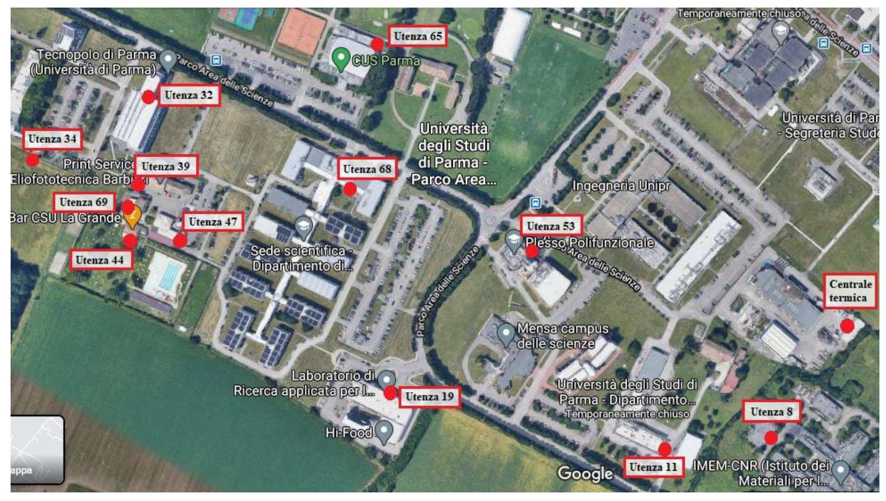
Parma University Campus is served by a DHC network, which is composed of four different sections. This study focuses on “Nuova Sud” heating branch: 4 km of extension, 12 buildings supplied, 12 MW total peak power, design temperatures of 80 °C/55 °C (supply/return), powered by natural gas boilers, and with 150,000 m3 of heated buildings. In order to maintain a temperature of 20 °C inside the rooms during the working hours, a by-pass valve regulates the water mass flow rate of each building [27]. A satellite view of the network is shown in Figure 1, where users are marked by an index that matches Table A1. More information is included in Appendix A.
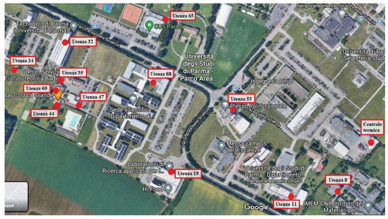
Figure 1.
Parma Campus–Users (“Utenza”) supplied by the “Nuova Sud” network, Source: Google Maps.
2.2. Modelling
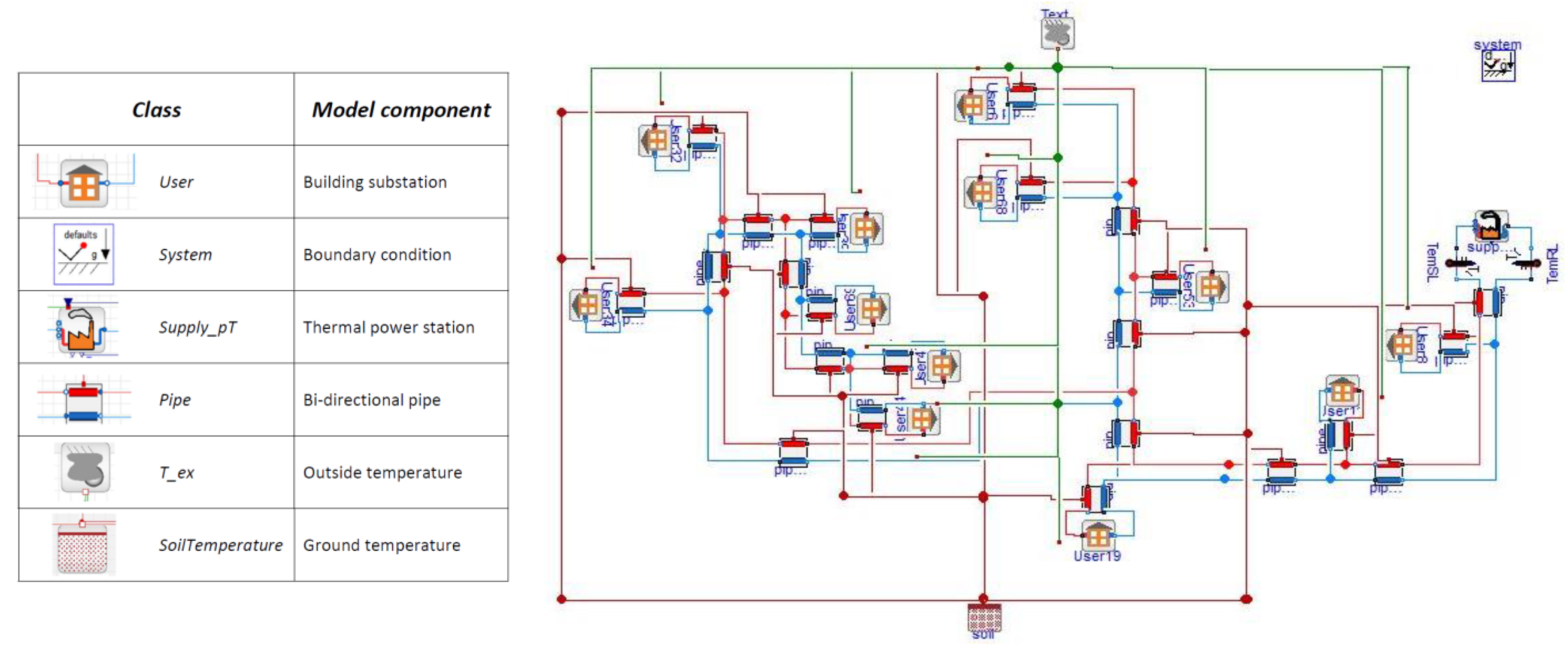
The network was simulated in a steady state to validate the model when the network is operating under its design conditions (ΔT = 25 °C at the user, 8.4/5 bar supply/return pressure, 80 °C supply temperature). In this case, the thermal energy supplied to the buildings was considered as a prescribed design value, and therefore no radiator terminals were modelled. Then, to investigate its dynamic behaviour during a whole heating season—considering variable thermal loads from each user—a specific model was implemented for the heat exchange between the secondary and the primary circuit, which requires the thermal load profiles characterising the demand of each user as an input. The model groups in a single section the branches going from the power plant to the junction, from the users to the junctions and between two junctions themselves. Actually, these are pipes with the same characteristics in terms of hydraulic diameter, thickness and type of material. The diagram view of the model realized in Dymola is presented in Figure 2.
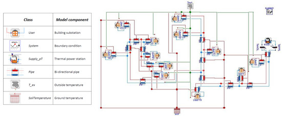
Figure 2.
Diagram view of the “Nuova Sud” district dynamic model in Dymola.
The components used for the network model are described in Table 1. Some were customised, starting from the existing classes available in the libraries “Modelica”, “IBPSA” and “DisHeatLib”. “DualDynamicPipe” models the fluid transport through pipes; the component solves differential equations by means of the finite volume method considering two nodes for each pipe (i.e., two mass balances, two energy balances and one momentum balance). The water is modelled as an incompressible fluid with prescribed physical characteristics, while the friction losses are calculated using the Swamee-Jain friction coefficient. Regarding the heat losses, they are computed by means of the constant heat transfer coefficient () that is detailed in Equations (1) and (2):
where is the thermal resistance of the pipe depending on its diameter (), length () and on its insulation characteristics, i.e., the thickness of the insulation layer () and the thermal conductivity of the insulation material ().

Table 1.
Overview of the components used for modelling the network.
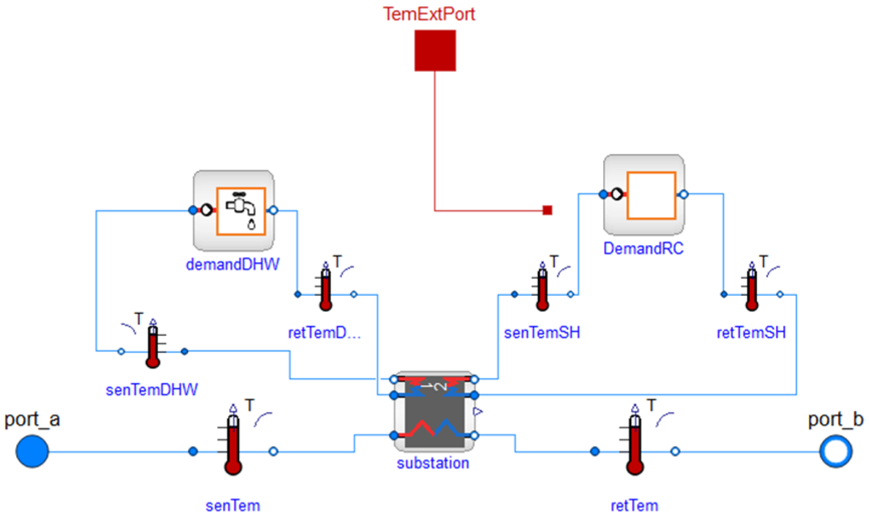
As for users, the component “BuildingIndirectStations” (Figure 3) models the thermal demand in dynamic conditions: secondary and primary circuit are coupled by an indirect heat exchange substation, modelled using the “DisHeatLib.Substations.SubstationParallel”; “DisHeatLib.Demand.Demand” components account thermal power demand for Domestic Heat Water (DHW, not modelled for this kind of user setting has a zero water mass flow rate circulating in the corresponding secondary branches) and Space Heating (SH). A PI controls the valve regulating the primary water mass flow rate going through the heat exchange: if the secondary water mass flow rate is different from zero, the supply temperature is set to the nominal value, whereas a minimum primary water mass flow rate is maintained if the secondary flow rate is zero (zero heat load). The heat exchange model is an ideal component (without a pressure drop) with an efficiency of 99%.
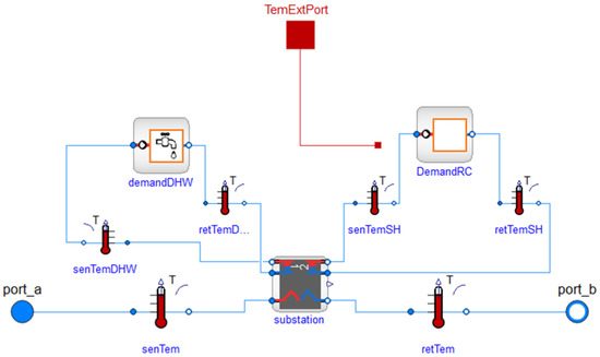
Figure 3.
Diagram view of “BuildingIndirectStations” model component in Dymola.
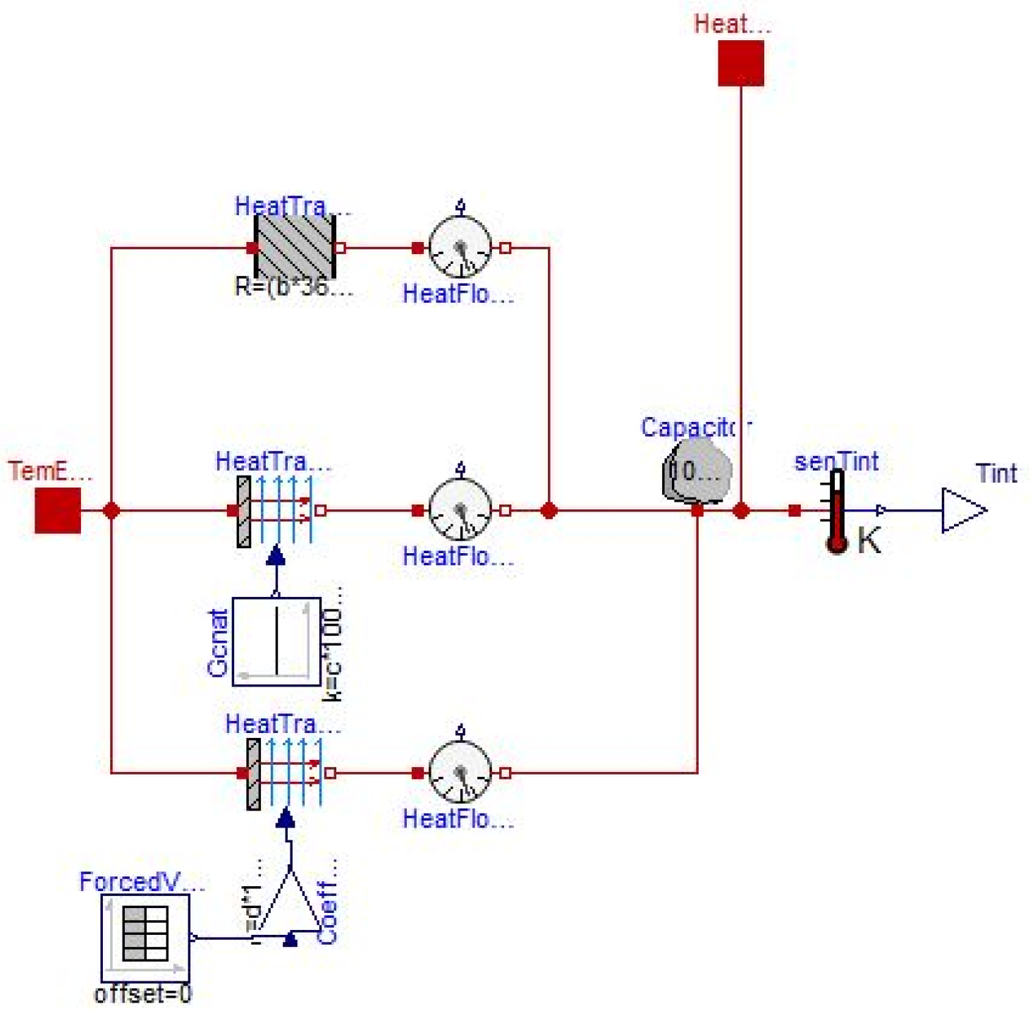
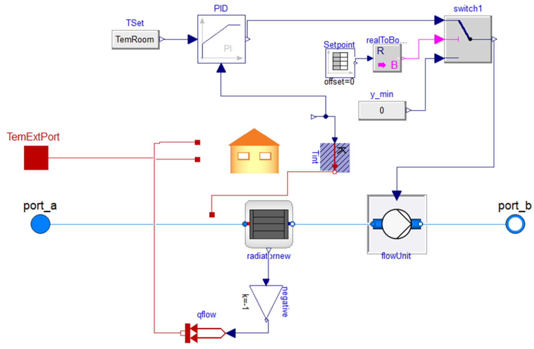
The results obtained from the given hourly heat requirements (under the following assumptions, the annual heating season in zone E [28] is from 15 October to 15 April; the heating service is from Monday to Friday, except for Palacampus (user 65), which is also heated on Saturdays), not included in this paper, show a good response from the model to the demand curve. A specific effort was dedicated to introducing a class that models the building behaviour with the use of thermophysical parameters, which describe different thermal exchanges [29]. In particular, the thermal power supplied to each building is no longer an input, and so a radiator model is introduced in the numerical simulations representing all of the terminals of in each building. The radiator component takes into account the dependence of the heat exchange on the mass flow rate and the temperature of primary and secondary circuits, and on the air temperature inside the building as well; therefore, based on this modelling approach, the total energy required by each user in order to maintain a given set point temperature becomes an output of the model. A new resistive-capacitive building model (“RCBuilding”, Figure 4) was introduced for implementing the dynamic energy balance of a building, detailed in Equations (3) and (4) [30]:
where is the air temperature inside the building, is the outside air temperature, is the overall thermal transmittance of the building envelope, is the area of the external walls, is the space heating power, is the heat transfer coefficient for natural ventilation, is the heat transfer coefficient for forced ventilation, is the mass of the building, and is a weighted average of the specific heat accounting the internal air and the walls. Coefficients in Equation (3) describe the temperature variation inside the building depending on the heat exchange through walls with the external environment (), the power input from the heating system (), the air infiltrations () and the forced ventilation with its air change rate (). Particularly, indicates the buildings’ ability to keep the energy stored inside, represents their thermal inertia, and relates the incoming air mass flow rate and specific heat with those of overall building systems; the specific values for each building in the network were obtained by the University of Parma with TRNSYS building models [29], as summarized in Table 2. Once validated through Simulink models in terms of heat exchanges and , “DemandSH” component has been modified in “DemandRC”, as shown in Figure 5. Here a radiator accounts for all of the terminal units of the building and its heat exchanges result in the heating load for each building, according to the control logic described below; the return temperature is calculated as a function of the supply temperature and (output of “RCBuilding”), according to the standard UNI EN 442-2. A PI controller compares the air temperature inside the building with the set point defined by the user. The output from PI is the input of a “switch” block, used to set the activation-deactivation time of temperature control, corresponding to the working hours: when the system is switched ON, it enables the PI to control the circulation pumps (“flowUnit”) on the secondary circuit; when OFF, pumps are supposed not operating. The heat exchanged between the transfer fluid and the environment is an input for the “RCBuilding” model; it can even manage air changes, by setting a specific timetable. A fine-tuning regulation of PI parameters was carried out according to the Ziegler-Nichols calibration method [31] (This action results in −3.70% of thermal energy supplied by the power plant, and −0.92% of pumping electricity, compared to the default PI values), in order to control the dynamics of the flow rate and temperature, both on the secondary (PI in the “RCDemand”) and on the primary (PI in the “IndirectStation”) circuits, and to avoid sudden power peaks in the heating plant as well.
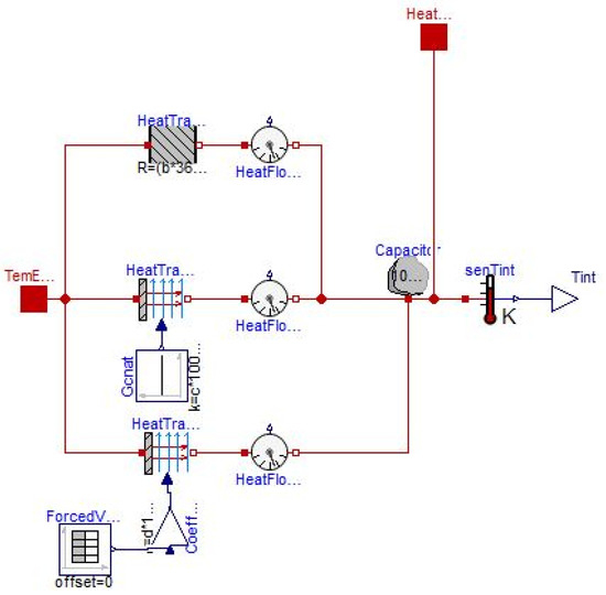
Figure 4.
Diagram view of “RCBuilding” model component in Dymola.
Table 2.
Performance coefficients of buildings supplied by “Nuova Sud” network.
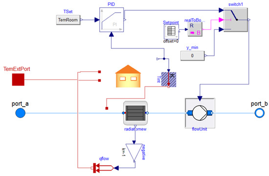
Figure 5.
Diagram view of “DemandRC” model component in Dymola.
Finally, the model component of the thermal power station (“Supply_pT”) is shown in Figure 6. Starting from a supply temperature input, which can be set to be constant or controlled by the external temperature, and a defined supply pressure, this results in the total required heat load and the electrical power supplied to the circulation pump.
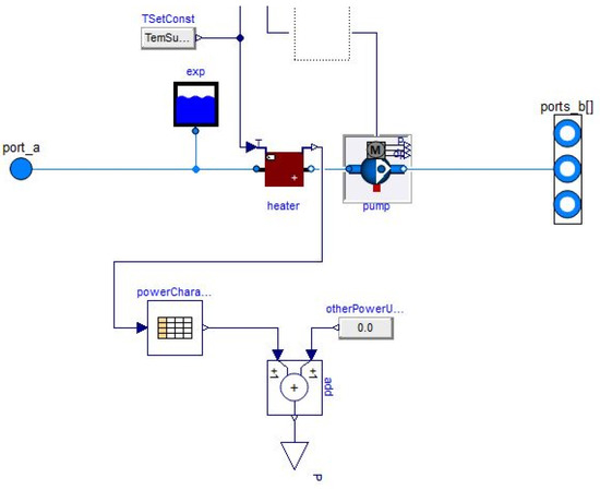
Figure 6.
Diagram view of “Supply_pT” model component in Dymola.
2.3. Simulations: Analysed Scenarios and Optimization
In order to optimise internal comfort conditions and, at the same time, to minimise energy consumption, different management scenarios were proposed and compared. A simulation time of eight weeks was chosen starting from the beginning of the heating season [28], i.e., at 00:00 on 15 October (2018 for weather conditions) in Parma, Italy [32]. All of the optimisation scenarios presented below have been modelled by modifying some parameters among the inputs set for the reference case (later, called Scenario 1) of the dynamic simulation, as described in Table 3.
Table 3.
Inputs of the Reference Case (Scenario 1) of dynamic simulation.
In detail, the analysed management scenarios are:
- Scenario 2—Early heating
According to the time delays observed in reaching the set-point temperature in the early hours of the morning, the space heating system in every user was set to be switched on 1 h earlier, i.e., at 6:00 am.
- Scenario 3—Heating system switched off for no-load condition
The supply temperature from the thermal power station is no more constant; the nominal value (80 °C) is maintained according to the Palacampus timetable, i.e., the user with the longer heating period. In this way, network dynamics can be observed when the fluid stops being heated.
- Scenario 4—Supply temperature depending on external conditions
In this scenario the supply temperature is set depending on the external temperature profile by means of a climatic curve, controlled according to conditions described by following Equations (5)–(7):
where is the supply temperature, ranging between the max and the min values, and is the external temperature, ranging between the max and the min values.
Aiming at defining an optimal scenario, the following parameters were taken into account: indoor comfort, in terms of the percentage of time, during the operating time of the heating plant, when the air temperature inside the building falls in a set comfort range (19 ÷ 21 °C); primary energy consumption i.e., fuel and electricity for pumping, related to thermal energy supplied to the network, quantified in tons of oil equivalent (toe) (the conversion coefficients are 0.836 toe for 1000 Sm3 of natural gas from FIRE (Italian Federation for the Rational Use of Energy), on the basis of point 13 of the explanatory note of the MiSE Circular of 18 December 2014 [33]; 0.171 toe for 1 MWh of electricity from the equivalent electrical efficiency of the Italian energy system in 2019 [34]).
Focusing on optimisation and management interventions, the economic assessment included cash flows related to the operational phase, not accounting for the profitability of a project for the new construction, extension, or modification of the existing network. The annual operative cost was estimated by the following Equation (8):
where is the fuel consumption [Sm3], is the electricity for pumping [kWhe], and is the energy from thermal central unit [kWht]. Here are the main assumptions:
- Average boiler efficiency 93% [35].
- Natural gas price. Reference values for fuel cost were provided by the Italian Regulatory Authority for Energy, Networks and Environment ARERA in terms of final prices for industrial consumers in 2019, divided for consumption slots: 57.06 c€/Sm3 (relative to the range 26,000–263,000 m3) equals to 58.69 €/MWh of primary energy, meaning 63.11 €/MWh of thermal energy fed into the grid.
- Electricity price. From the same reference a value of 22.25 c€/kWhe was selected for the range 50–500 MWhe as electricity cost .
- Operation and maintenance costs were estimated per thermal unit supplied by the central heating plant, i.e., 1.9 €/MWht and 3 €/MWht, respectively [36], and were not affected by the different scenarios because they did not modify the existing network.
Not knowing the emission factor of the district heating of Parma, the environmental assessment was performed by accounting for emissions associated to the combustion of natural gas in boilers and electricity from the national grid (, as shown by Equation (9):
where:
- National standard parameters proposed by the Ministry of the Environment were used as a reference for the emission factor of fuel combustion . These include the coefficients used for the CO2 emissions in the UNFCCC national inventory, as an average of the values of the years 2017–2019 [37]: 1.984 tCO2/1000 Sm3 or 56.231 tCO2/TJ, which is 204 gCO2/kWh, assuming 1 as oxidation coefficient.
- Emission factor for electricity does not consider imported energy, but accounts for the network losses, according to [38], resulting in 305 gCO2/kWhe in 2019 [34].
Once the robustness of the models, the coupling of hydraulic and energy problems and the possibility of editing the thermo-physical characteristics of buildings were verified, the activity continued on the evaluation of deep renovation interventions, including their effects in terms of energy savings, operating temperature level, lower supply temperature and heat losses in the network, and the consequently higher electricity consumption of pumping. Through a simplified network model, the ex-ante and ex-post performances are compared in both operating conditions of the network, i.e., traditional and low temperature. The installation of polyurethane foam (10 cm, 0.026 W/m2K) to the external facades of user 39 was modelled by modifying the parameters and accordingly (−75.26% and −99.98%); final transmittance complies with the current legislation for accessing incentive mechanisms.
3. Results and Discussion
The dynamic model simulation results in flow rates, temperatures, pressures and losses along the network, the temperature inside every building, control records, the thermal power and energy supplied to the users, and the energy balance in the central heating system, including electricity for pumping uses.
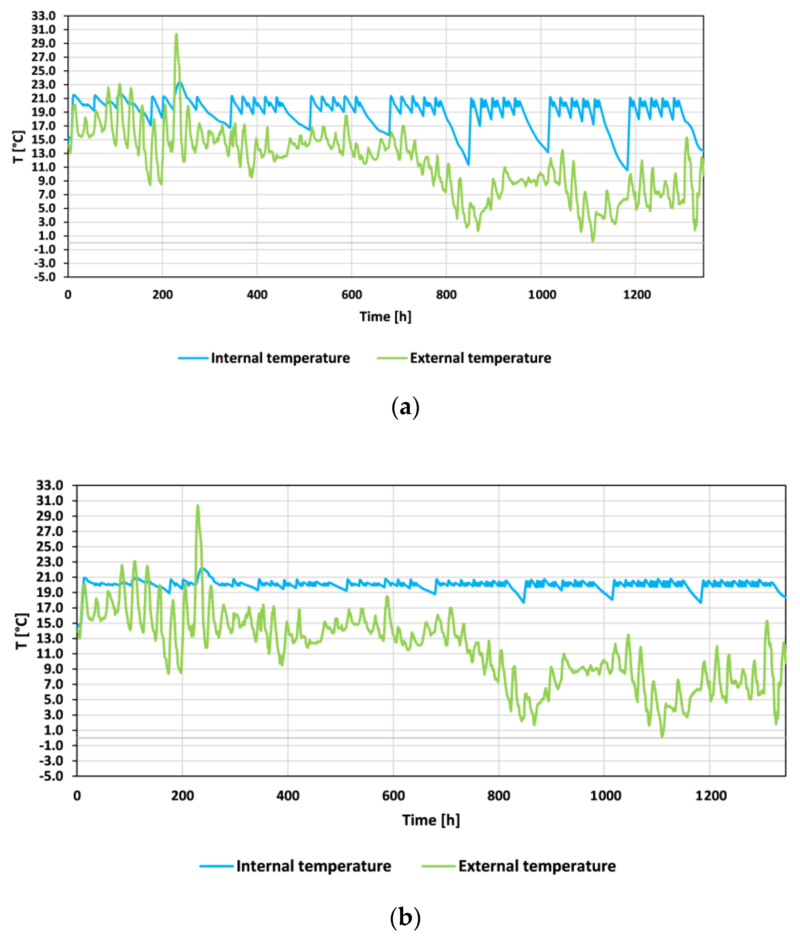
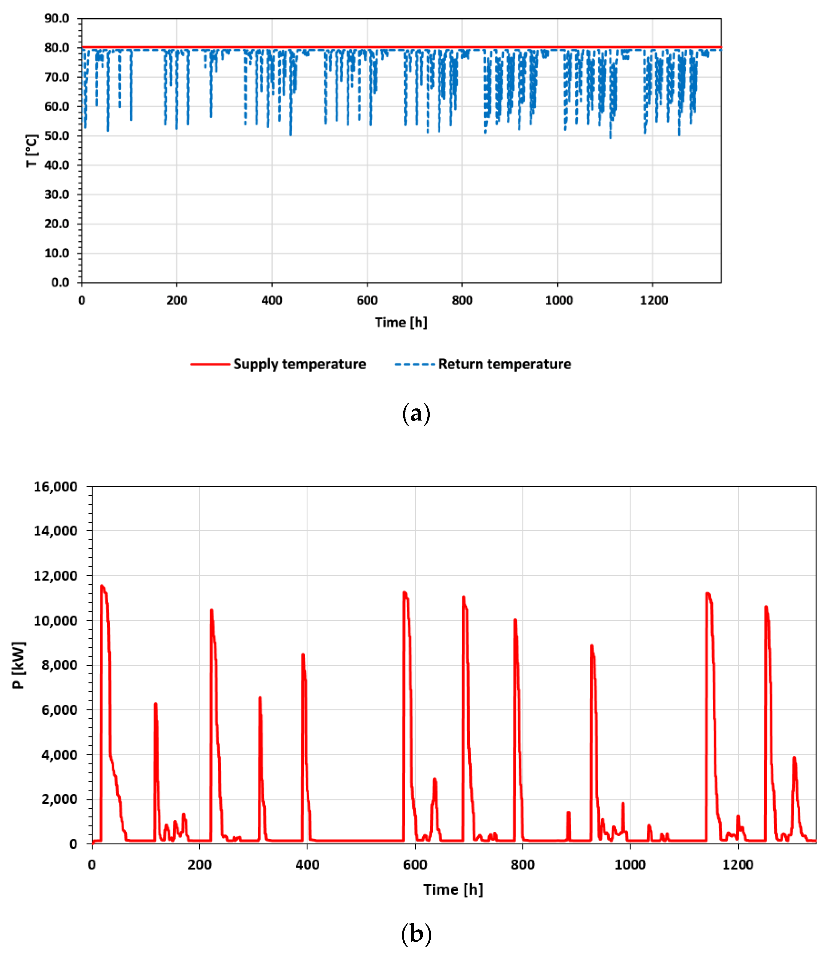
Focusing on reference case (Scenario 1), the temperature inside the buildings depends on the external temperature profile: at the beginning of the season, peaks are often coupled with . However different performance parameters for the buildings affect trends: the historical archive (user 8) is characterised by an parameter that is approximately 5.2 times greater than Palacampus (user 65), resulting in a thermodynamic behaviour that is more energy efficient for the latter. Figure 7 show how Palacampus is able to better maintain the set-point imposed during the hours when the heating system is on. The supply temperature is kept constant, while the return temperature varies according to the heating loads and the energy losses along the network, as shown in Figure 8; it includes the power supplied by the central heating system.

Figure 7.
Scenario 1—External (green) and internal (blue) temperatures [°C], for user 8 (a) and user 65 (b) along the simulation time [h].

Figure 8.
Scenario 1—Central heating system along the simulation time [h]: (a) supply (red) and return (blue) temperatures [°C], (b) power supplied to the network [kW].
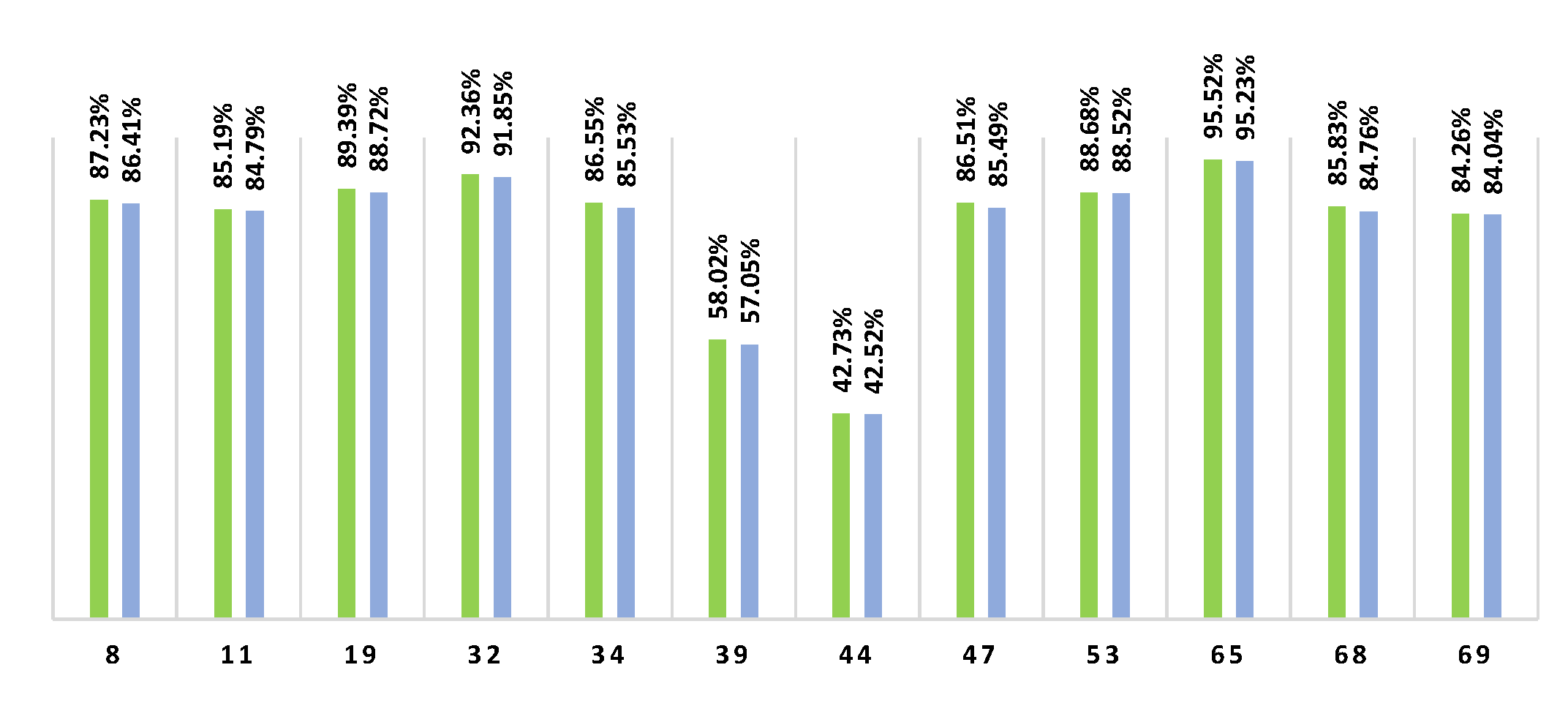
Moving to the other management sets for a comparative assessment, Scenario 2–as expected–shows the best results in terms of inner temperature. As thermal conditions are closely related to the thermo-physical characteristics of the buildings, most problematic users in the reference case benefit from improved comfort conditions; the percentage of time in which the air is between 19 °C and 21 °C increases from 57.56% to 65.32% and from 58.90% to 66.72%, respectively, for users 39 and 44, as shown in Figure 9. Regarding Scenarios 3 and 4, the percentages remain very similar to the values of the reference case, meaning that the variations in supply temperature do not affect the much, unlike heat losses. As expected, turning on the heating system earlier (Scenario 2) improves comfort conditions and results in higher energy consumption (+0.89%) and costs (+0.85%, Figure 10) as well. The most energy efficient scenarios are Scenarios 3 and 4, with toe energy saving of 1.14% and 1.41%, respectively (Table 4)). However, the components that contribute to the achievement of the total energy consumption vary differently in these scenarios: on one hand, modulating the supply temperature in the plant depending on (Scenario 4) decreases fuel consumption (−2.34%); on the other hand, a lower temperature level causes higher consumption of electricity for pumping uses (+12.96%), resulting in a reduction in overall expenditure of 0.76%. This does not happen in the case where the flow temperature constant is kept at 80 °C only during working hours (Scenario 3), as the pumps continue to consume the same energy as in the reference scenario with a consequent reduction in economic expenditure of 1.09%. The network heat losses decrease for both Scenario 3 and Scenario 4 by 5.89% and 8.91%, respectively, with a greater potential economic valorisation of the heat produced in Scenario 3. Regarding GHG emissions, as expected, they follow the energy consumption trend: +0.90% for Scenario 2, −1,16% for Scenario 3, and −1.59% for Scenario 4.
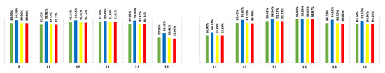
Figure 9.
Indoor temperature according to the set-point 19 ÷ 21 °C, percentage of time in different users, comparison of scenarios (Scenario 1 in green, Scenario 2 in blue, Scenario 3 in yellow, and Scenario 4 in red).
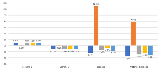
Figure 10.
Relative changes from the reference case/scenario, in terms of supplied thermal energy (blue), electricity for pumping (orange), overall operating sources (grey), cost (yellow), and CO2 emissions (light blue).
Table 4.
Energy, economic and environmental assessment (in grey field those considered as reference for the comparative analysis).
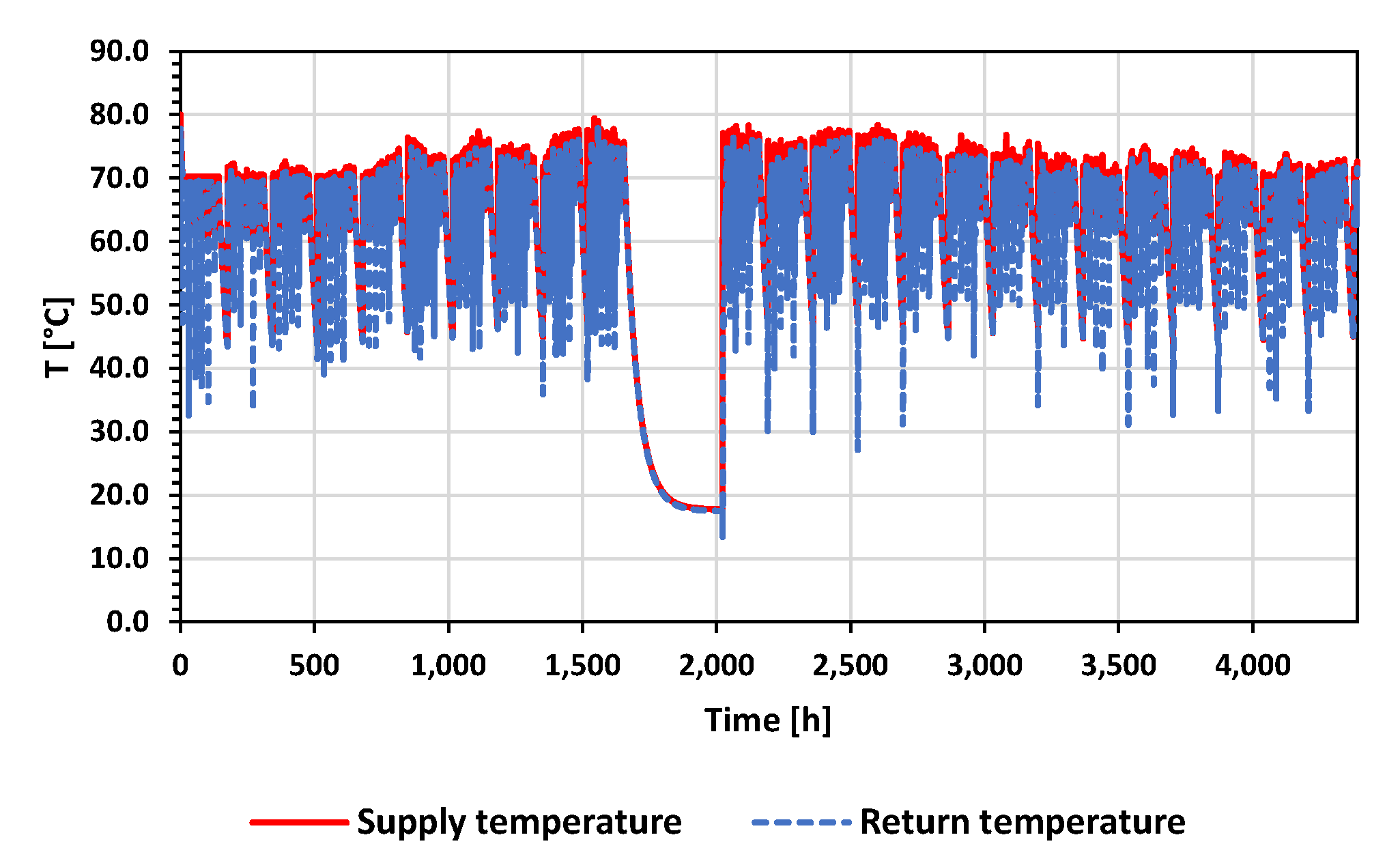
Scenarios 3 and 4 result in energy savings that maintain comfort percentages that are not far from the best values of Scenario 2. As such, a simulation for the entire heating season was performed in order to compare the reference scenario and a new management set, called the “optimised scenario”, where the benefits from turning off the supply in the case of no thermal demand (Scenario 3) and those due to the modulation of supply temperature (Scenario 4) are combined together. The heating season includes two weeks for winter holidays during which the central heating generation is turned off, and implementing a control on fluid temperature (set >5 °C). Figure 11 shows the supply and return temperature in the optimised scenario: during the winter holidays, the temperature of fluid in the network decreases until it reaches 18 °C. During the operating time, the average supply and return temperatures are lower compared to the reference scenario, with lower heat losses, unlike the higher values for mass flow rates and pumping energy. The performance in terms of the indoor air temperature is slightly reduced for the optimised scenario (Figure 12), although the differences are in the order of 1%. As for energy consumption, Table 4 shows that the optimised scenario decreases the thermal energy supplied by the power plant by 3.54%, with a −17.83% of thermal energy losses; even if the pumping requirement increases by 7.76%, the overall energy consumption (toe) and emissions (CO2) lower by 2.86% and 3.02%, respectively. Therefore, the optimised scenario results in lower energy consumption, and does not significantly affect the thermal comfort conditions inside the buildings. The recent extraordinary dynamics at the international level of commodity prices (related to increases in raw materials and CO2 allowances, leading to +70% for natural gas and +20% for electricity) affect the economic assessment, with a +60% in operating costs, whereas the relative reduction of the optimised scenario moves from 2.40% to 2.70%.

Figure 11.
Optimised scenario–Central heating system along the entire heating season [h]: supply (red) and return (blue) temperature [°C].
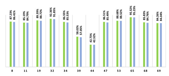
Figure 12.
Indoor temperature according to the set-point 19 ÷ 21 °C, percentage of time in different users: reference scenario in green, optimized scenario in light blue.
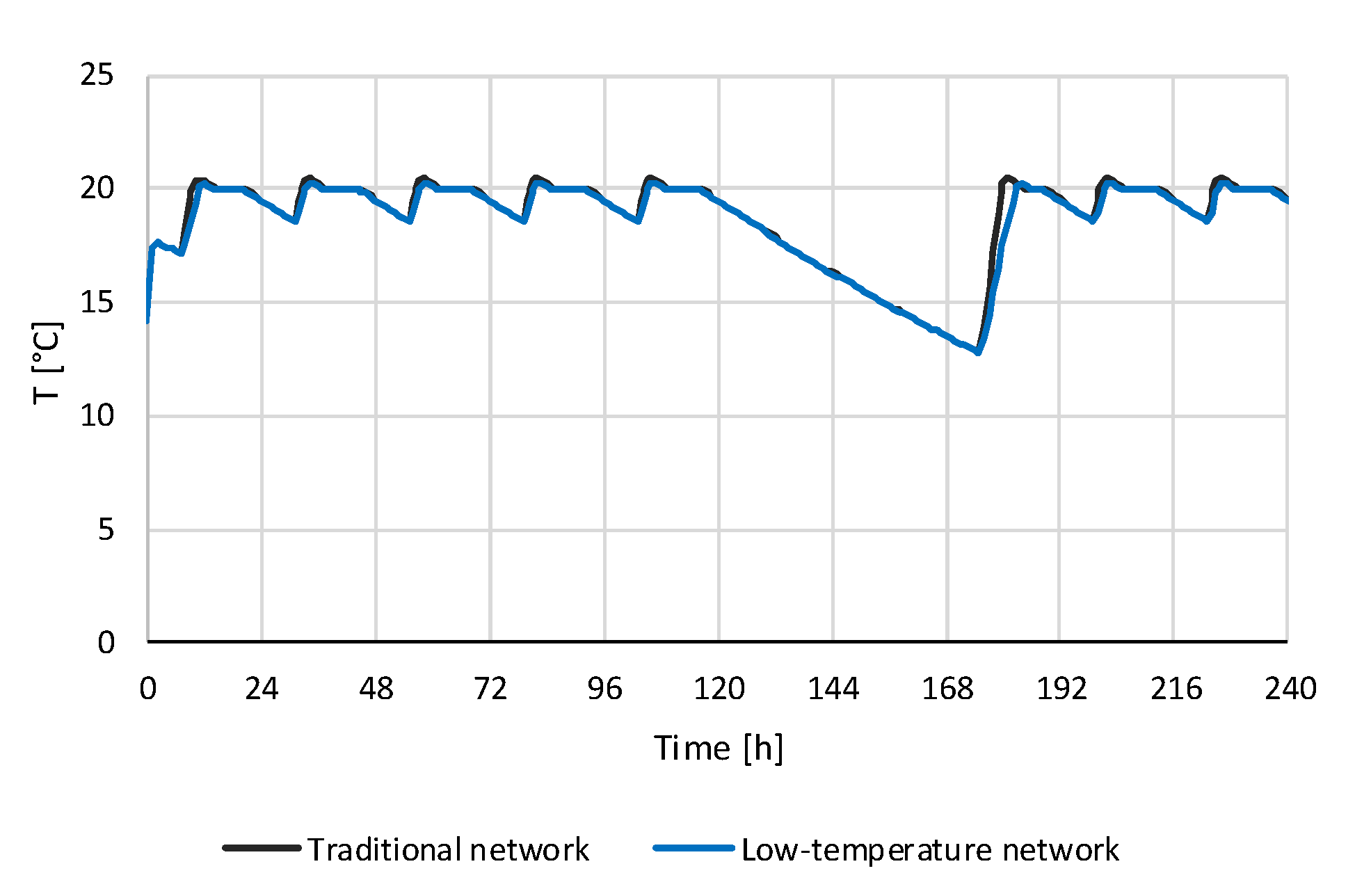
Finally, a simplified network was modelled in order to highlight the benefits related to a deep renovation of a single user (i.e., no. 39, penalised by its thermos-physical features–ten days simulation); an increased thermal insulation results in lower consumptions and heat losses from the building to reach comfort conditions, and in increased minimum values for the return temperature in the network (Figure 13). In particular, the supplied thermal energy and electricity consumption for pumping decrease by 56.70% and 23.71% respectively, and the energy losses decreases as well by 3%. A further comparison was made by lowering the supply temperature in the network to 55 °C (30 °C for return). The results show similar profiles of internal temperature and consequent good comfort conditions (Figure 14), against −22.38% of supplied thermal energy, +3.28% of pumping electricity, and a remarkable −28.11% of heat losses. These results reflect the multi-physics of the district heating, even if not directly comparable with other studies with different configurations, e.g., RES integration in [13]. These promising preliminary results may be extended in the future to analyse the operation of the entire network, and further investigations will include the dependency of thermal efficiency on central heater (e.g., condensing boilers) and supply temperature.
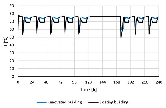
Figure 13.
Return temperature [°C], for the original (black) and the renovated building (blue), along the simulation time [h].

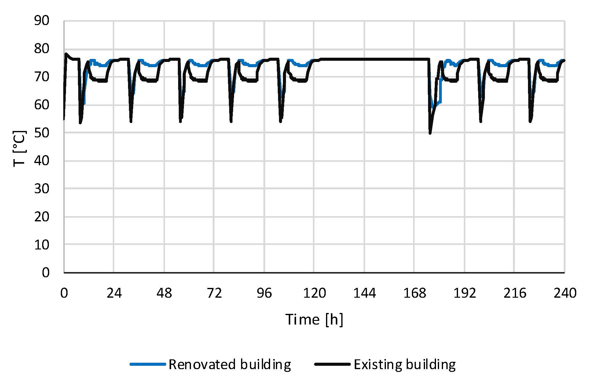
Figure 14.
Renovated building–Internal temperature [°C], for traditional (black) and low-temperature (blue) network, along the simulation time [h].
4. Conclusions
EU Directive 2018/2001 emphasises the role of district heating and cooling in the renewable energy penetration on power system, providing limits on RES share and waste heat and cold sources in final energy consumption. District heating is intended to cover a reducing overall demand of primary energy in building sector–due to the decarbonisation targets–related to the renovation of existing buildings, with operating temperatures expected to be lower than traditional networks, and to integrate low–medium temperature heat sources (to convey the excess energy produced by RES non-programmable or to recover waste heat) with active exchange substations. In this framework, retrofitting interventions of existing networks moves from temperature optimisation and management actions towards fourth generation district heating networks (50–55 °C and 30–35 °C for supply and return temperatures respectively), an efficient solution applicable to an increasing share of the building stock for improving the efficiency in transport and distribution with consequent cost and environmental benefits. A lower temperature influences the production system, heat losses and electricity required for the pumping system, and introduces the possibility of using a number of additional local heat sources. In order to investigate effective management measures, a model was developed to simulate the energy and hydraulic behaviour operating in real conditions; this overcomes the limitations of previous models in terms of network layout and hydraulic analysis (e.g., absence of the bidirectional motion of the fluid in the pipe section). It was applied to the district heating network of Parma University: starting from a single user in stationary conditions, activities focused on the entire dynamic network, introducing a tailored resistive-capacitive model for buildings; once identified appropriate PI parameters and set the control logics, a number of simulation were performed on different management scenarios, in order to find out the trading point between energy consumption and indoor comfort conditions for the heating season; finally, the assessment was extended to a possible renovation scenario and low-temperature management of the network. Energy, economic, and environmental results support possible future in-depth investigations, concerning specific technological innovations, as suggested in [39]: digitalisation, i.e., introduction of smart systems for data collection about heat demand and monitoring systems; alternative piping options; improvements at private buildings (e.g., heat exchangers of substations, terminals in the users, etc.) and the introduction of decentralised storage tanks. Retrofitting interventions of existing networks is supported in the legislative framework defined in the National Integrated Energy and Climate Plan; the mechanisms currently available for promoting the new construction and the expansion of infrastructure will be strengthened, e.g., subsidies will be provided for interventions aimed at maintaining or achieving an “efficient” district heating system (according to Directive 2012/27/EU) through increased heat production, combined with an extension of the network in terms of increased transport capacity.
Author Contributions
Conceptualization, M.R., P.S., S.T., M.A.A. and F.M.; methodology, M.R., P.S., S.T., M.A.A. and F.M.; software and simulation, M.R., S.T. and E.D.D.; formal analysis, M.R., P.S., S.T. and E.D.D.; data curation, M.R., P.S., S.T., E.D.D. and M.A.A.; writing—original draft preparation, P.S., E.D.D. and M.A.A.; writing—review and editing, M.R., P.S., E.D.D. and M.A.A.; supervision, G.P. and F.M.; project administration, P.S. and G.P.; funding acquisition, G.P. All authors have read and agreed to the published version of the manuscript.
Funding
This research was funded in the Program Agreement between the Italian National Agency for New Technologies, Energy and Sustainable Economic Development (ENEA) and the Ministry of Economic Development (now Ministry of Ecological Transition) for Electric System Research, in the framework of its Implementation Plan for 2019–2021. In particular, the activity is included in the Project 1.5 “Technologies, techniques and materials for energy efficiency and energy savings in the electrical end uses of new and existing buildings”, Work Package 4 “Integrated Energy Networks”.
Informed Consent Statement
Not applicable.
Data Availability Statement
More information about Electric System Research and its Implementation Plan for 2019–2021 are available at http://www.ricercadisistema.it/ (accessed on 11 November 2021, Italian language).
Acknowledgments
Authors would like to thank Mirko Morini, associate in Fluid Machinery at the Department of Engineering and Architecture of the University of Parma, and his research group for providing network features.
Conflicts of Interest
The authors declare no conflict of interest. The funders had no role in the design of the study; in the collection, analyses, or interpretation of data; in the writing of the manuscript, or in the decision to publish the results.
Appendix A
The network topology is shown in Figure A1, while the supplied buildings are listed in Table A1. The pipe diameters are given in Table A2, together with the lengths of each branch, the thickness of the thermal insulation and its thermal conductivity.
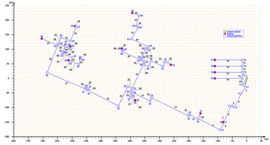
Figure A1.
Network topology [25].
Figure A1.
Network topology [25].
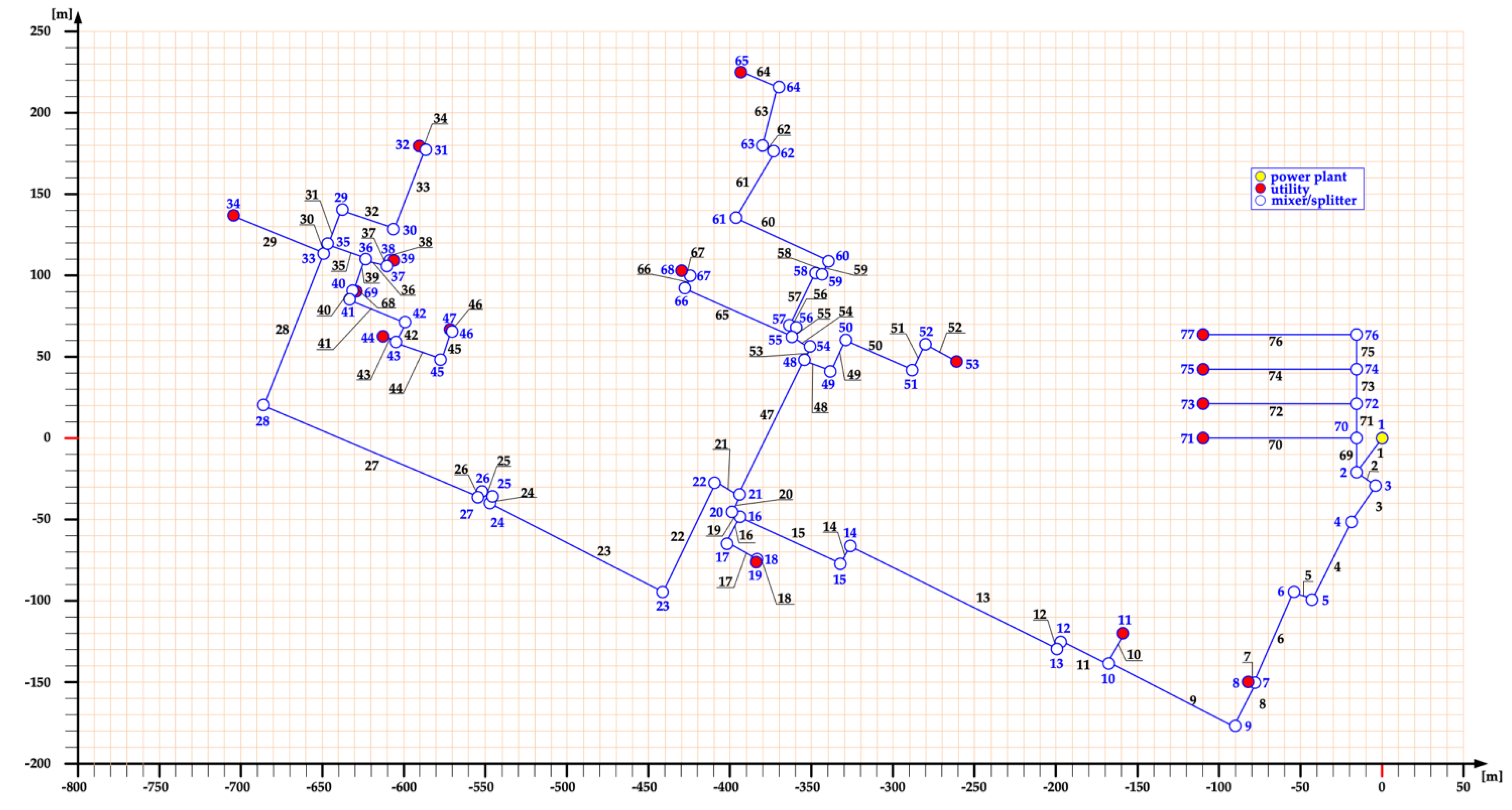
Table A1.
Buildings supplied by the “Nuova Sud” network.
Table A1.
Buildings supplied by the “Nuova Sud” network.
| User ID | User Description |
|---|---|
| 8 | History Archive |
| 11 | Food Science |
| 19 | Materials Laboratory |
| 32 | Technopole |
| 34 | Earth Science |
| 39 | Big Print Shop Centre |
| 44 | Bar |
| 47 | Big Church Centre/Classrooms |
| 53 | Multipurpose Centre/Auditorium |
| 65 | Palacampus |
| 68 | Science Engineering |
| 69 | Cafeteria |
Table A2.
Network technical features.
Table A2.
Network technical features.
| Branch | Pipe Diameters [m] | Thermal Insulation Thickness [mm] | Thermal Conductivity [W/(mK)] | Length [m] |
|---|---|---|---|---|
| 1_7 | 0.200 | 47.95 | 0.040 | 193.46 |
| 7_8 | 0.080 | 35.55 | 0.040 | 4.12 |
| 7_10 | 0.200 | 47.95 | 0.040 | 115.81 |
| 10_11 | 0.080 | 35.55 | 0.040 | 20.53 |
| 10_16 | 0.200 | 47.95 | 0.040 | 259.46 |
| 16_19 | 0.080 | 35.55 | 0.040 | 40.94 |
| 16_21 | 0.200 | 47.95 | 0.040 | 17.40 |
| 21_33 | 0.200 | 47.95 | 0.040 | 469.76 |
| 33_34 | 0.125 | 42.65 | 0.040 | 60.04 |
| 33_35 | 0.200 | 47.95 | 0.040 | 6.64 |
| 35_32 | 0.100 | 42.85 | 0.040 | 113.57 |
| 35_36 | 0.125 | 42.65 | 0.040 | 25.22 |
| 36_39 | 0.110 | 42.50 | 0.040 | 19.98 |
| 36_40 | 0.125 | 42.65 | 0.040 | 20.93 |
| 40_69 | 0.100 | 42.85 | 0.040 | 2.20 |
| 40_43 | 0.125 | 42.65 | 0.040 | 55.78 |
| 43_44 | 0.110 | 42.50 | 0.040 | 8.68 |
| 43_47 | 0.110 | 42.50 | 0.040 | 49.96 |
| 21_48 | 0.200 | 47.95 | 0.040 | 91.82 |
| 48_53 | 0.100 | 42.85 | 0.040 | 123.45 |
| 48_55 | 0.200 | 47.85 | 0.040 | 21.50 |
| 55_68 | 0.150 | 41.00 | 0.040 | 86.61 |
| 55_65 | 0.100 | 42.85 | 0.040 | 235.54 |
References
- Smith, M.S.; Cook, C.; Sokona, Y.; Elmqvist, T.; Fukushi, K.; Broadgate, W.; Jarzebski, M.P. Advancing sustainability science for the SDGs. Sustain. Sci. 2018, 13, 1483–1487. [Google Scholar] [CrossRef] [PubMed]
- Connolly, D.; Lund, H.; Mathiesen, B.V.; Werner, S.; Möller, B.; Persson, U.; Boermans, T.; Trier, D.; Østergaard, P.A.; Nielsen, S. Heat Roadmap Europe: Combining district heating with heat savings to decarbonise the EU energy system. Energy Policy 2014, 65, 475–489. [Google Scholar] [CrossRef]
- Proposal for a Regulation of the European Parliament and of the Council Establishing the Framework for Achieving Climate Neutrality and Amending Regulation (EU) 2018/1999 (European Climate Law). Available online: https://eur-lex.europa.eu/legal-content/EN/TXT/?qid=1588581905912&uri=CELEX:52020PC0080 (accessed on 15 November 2021).
- Fernández, M.G.; Bacquet, A.; Bensadi, S.; Morisot, P.; Oger, A. Integrating Renewable and Waste Heat and Cold Sources into District Heating and Cooling Systems; Publications Office of the European Union: Luxembourg, 2021; ISBN 978-92-76-29428-3. Available online: https://publications.jrc.ec.europa.eu/repository/handle/JRC123771 (accessed on 15 November 2021). [CrossRef]
- Margaritis, N.; Rakopoulos, D.; Mylona, E.; Grammelis, P. Introduction of renewable energy sources in the district heating system of Greece. Int. J. Sustain. Energy Plan. 2014, 4, 43–55. [Google Scholar] [CrossRef]
- Sartor, K.; Quoilin, S.; Dewallef, P. Simulation and optimization of a CHP biomass plant and district heating network. Appl. Energy 2014, 130, 474–483. [Google Scholar] [CrossRef] [Green Version]
- Schmidt, R.F.; Fevrier, N.; Dumas, P. Smart cities and Communities, Key to Innovation Integrated Solution—Smart Thermal Grids. 2013. Available online: http://www.rhc-platform.org/fileadmin/2013_RHC_Conference/Presentations/Tuesday_23rd_April/Session_G/1/Philippe_Dumas_Smart_cities_-_Solution_Proposal_Smart_thermal_grid.pdf (accessed on 15 November 2021).
- Schmidt, D. Low Temperature District Heating for Future Energy Systems. Energy Procedia 2018, 149, 595–604. [Google Scholar] [CrossRef]
- Lund, H.; Werner, S.; Wiltshire, R.; Svendsen, S.; Thorsen, J.E.; Hvelplund, F.; Mathiesen, B.V. 4th Generation District Heating (4GDH): Integrating smart thermal grids into future sustainable energy systems. Energy 2014, 68, 1–11. [Google Scholar] [CrossRef]
- Østergaard, D.S.; Svendsen, S. Costs and benefits of preparing existing Danish buildings for low-temperature district heating. Energy 2019, 176, 718–727. [Google Scholar] [CrossRef]
- Sarbu, I.; Sebarchievici, C. Using Ground-Source Heat Pump Systems for Heating/Cooling of Buildings. In Advances in Geothermal Sciences; IntechOpen Limited: London, UK, 2016; Chapter 1. [Google Scholar] [CrossRef] [Green Version]
- Reguis, A.; Vand, B.; Currie, J. Challenges for the Transition to Low-Temperature Heat in the UK: A Review. Energies 2021, 14, 7181. [Google Scholar] [CrossRef]
- Ancona, M.A.; Bianchi, M.; Branchini, L.; De Pascale, A.; Melino, F.; Peretto, A. Low-temperature district heating networks for complete energy needs fulfillment. Int. J. Sustain. Energy Plan. Manag. 2019, 24, 33–42. [Google Scholar] [CrossRef]
- Gestore dei Servizi Energetici GSE S.p.A. (Italian Energy Services Manager). District Heating and Cooling 2019—Networks and Supplied Energy in Italy. 2021. Available online: https://www.gse.it/documenti_site/Documenti%20GSE/Rapporti%20statistici/Nota%20TLR%202021%20-%20GSE.pdf (accessed on 15 November 2021).
- Italian Legislative Decree No. 102 of 4 July 2014 Implementing Directive 2012/27/EU on Energy Efficiency, Amending Directives 2009/125/EC and 2010/30/EU and Repealing Directives 2004/8/EC and 2006/32/EC, Official Journal General Series No. 165 18 July 2014. Available online: https://www.gazzettaufficiale.it/eli/id/2014/07/18/14G00113/sg (accessed on 15 November 2021).
- Italian Ministry of Economic Development, Decree 5 September 2011, New Support Scheme for High-Efficiency Cogeneration, Official Journal General Series No. 218 19 September 2011. Available online: https://www.mise.gov.it/index.php/it/ (accessed on 15 November 2021).
- Ancona, M.A.; Branchini, L.; De Pascale, A.; Melino, F. Smart district heating: Distributed generation systems’ effects on the network. Energy Procedia 2015, 75, 1208–1213. [Google Scholar] [CrossRef] [Green Version]
- Ben Hassine, I.; Eicker, U. Control aspects of decentralized solar thermal integration into district heating networks. Energy Procedia 2014, 48, 1055–1064. [Google Scholar] [CrossRef] [Green Version]
- Résimont, T.; Louveaux, Q.; Dewallef, P. Optimization Tool for the Strategic Outline and Sizing of District Heating Networks Using a Geographic Information System. Energies 2021, 14, 5575. [Google Scholar] [CrossRef]
- Delgado, B.M.; Kotireddy, R.; Cao, S.; Hasan, A.; Hoes, P.J.; Hensen, J.; Sirén, K. Lifecycle cost and CO2 emissions of residential heat and electricity prosumers in Finland and the Netherlands. Energy Convers. Manag. 2018, 160, 494–508. [Google Scholar] [CrossRef] [Green Version]
- Wang, H.; Wang, H.; Zhou, H.; Zhu, T. Modeling and optimization for hydraulic performance design in multisource district heating with fluctuating renewables. Energy Convers. Manag. 2018, 156, 113–129. [Google Scholar] [CrossRef]
- Carpaneto, E.; Lazzeroni, P.; Repetto, M. Optimal integration of solar energy in a district heating network. Renew. Energy 2015, 75, 714–721. [Google Scholar] [CrossRef]
- Huber, D.; Illyés, V.; Turewicz, V.; Götzl, G.; Hammer, A.; Ponweiser, K. Novel District Heating Systems: Methods and Simulation Results. Energies 2021, 14, 4450. [Google Scholar] [CrossRef]
- Vaisi, S.; Mohammadi, S.; Habibi, K. Heat Mapping, a Method for Enhancing the Sustainability of the Smart District Heat Networks. Energies 2021, 14, 5462. [Google Scholar] [CrossRef]
- Delubac, R.; Serra, S.; Sochard, S.; Reneaume, J.-M. A Dynamic Optimization Tool to Size and Operate Solar Thermal District Heating Networks Production Plants. Energies 2021, 14, 8003. [Google Scholar] [CrossRef]
- Corradi, E.; Rossi, M.; Mugnini, A.; Nadeem, A.; Comodi, G.; Arteconi, A.; Salvi, D. Energy, Environmental, and Economic Analyses of a District Heating (DH) Network from Both Thermal Plant and End-Users’ Prospective: An Italian Case Study. Energies 2021, 14, 7783. [Google Scholar] [CrossRef]
- Ancona, M.A.; Branchini, L.; De Lorenzi, A.; De Pascale, A.; Gambarotta, A.; Melino, F.; Morini, M. Application of different modeling approaches to a district heating network. AIP Conf. Proc. 2019, 2191, 020009. [Google Scholar] [CrossRef]
- Italian Presidential Decree 26 August 1993, No. 412, Regulation on Standards for the Design, Installation, Operation and Maintenance of Heating Systems in Buildings Aimed at Limiting Energy Consumption, in Implementation of Art. 4, Paragraph 4, of Law 9 January 1991, No. 10. Official Journal General Series No. 242 14 October 1993. Available online: https://www.gazzettaufficiale.it/eli/id/1993/10/14/093G0451/sg (accessed on 15 November 2021).
- Stonfer, M.; Morini, M.; Gambarotta, A.; Rossi, M. Development of a Dynamic Model for the Simulation of District Heating Networks in a Smart Energy Perspective and Application to the University Campus. Master’s Thesis, University of Parma, Parma, Italy, 2016. [Google Scholar]
- Saletti, C.; Zimmerman, N.; Morini, M.; Kyprianidis, K.; Gambarotta, A. A control-oriented scalable model for demand side management in district heating aggregated communities. Appl. Therm. Eng. 2022, 201, 117681. [Google Scholar] [CrossRef]
- Ziegler, J.G.; Nichols, N.B. Optimum Settings for Automatic Controllers. J. Dyn. Syst. Meas. Control 1993, 115, 220–222. [Google Scholar] [CrossRef]
- Agency for Prevention, Environment and Energy Emilia-Romagna ARPAE, Dexter. Available online: https://simc.arpae.it/dext3r (accessed on 15 November 2021).
- Italian Ministry for Economic Development (MiSE), Circular 18 December 2014, New Ways of Appointing Energy Managers. Available online: https://www.mise.gov.it/index.php/it/energia/efficienza-energetica/94-normativa/circolari,-note,-direttive-e-atti-di-indirizzo/2031968-circolare-del-18-dicembre-2014-nuove-modalita-di-nomina-degli-energy-manager (accessed on 15 November 2021).
- Caputo, A. Indicators of Efficiency and Decarbonization of the National Energy and Power System; Italian Superior Institute for Environmental Protection and Research (ISPRA): Rome, Italy, 2021; ISBN 978-88-448-1049-8. [Google Scholar]
- Sdringola, P.; Proietti, S.; Astolfi, D.; Castellani, F. Combined Heat and Power Plant and District Heating and Cooling Network: A Test-Case in Italy with Integration of Renewable Energy. ASME J. Sol. Energy Eng. 2018, 140, 5. [Google Scholar] [CrossRef]
- Gestore dei Servizi Energetici GSE S.p.A. (Italian Energy Services Manager). Assessment of National and Regional Potential for Application of High-Efficiency Cogeneration and Efficient District Heating, Dossier in Compliance with Article 10 of Legislative Decree 102/2014 Implementing the Energy Efficiency Directive 2012/27/EU, December 2016. Available online: https://www.gse.it (accessed on 15 November 2021).
- Italian Ministry of the Environment, Land and Sea Protection, National Standard Parameters—Coefficients Used for CO2 Emissions Inventory in the UNFCCC National Inventory (Average of Values for the Years 2017–2019). Available online: https://www.ets.minambiente.it/News#201-pubblicazione-parametri-standard-nazionali-anno-2020 (accessed on 15 November 2021).
- Caserini, S.; Baglione, P.; Cottafava, D.; Gallo, M.; Laio, F.; Magatti, G.; Maggi, V.; Maugeri, M.; Moreschi, L.; Perotto, E.; et al. CO2 emission factors for energy consumption and transport for the greenhouse gas inventories of Italian universities. Ing. Dell’ambiente 2019, 6, 43–59. [Google Scholar] [CrossRef]
- H2020, European Project TEMPO Temperature Optimisation for Low Temperature District Heating across Europe, H2020-EE-2017-RIA-IA. Grant Agreement ID: 768936. Available online: https://www.tempo-dhc.eu/ (accessed on 15 November 2021).


Publisher’s Note: MDPI stays neutral with regard to jurisdictional claims in published maps and institutional affiliations. |
© 2022 by the authors. Licensee MDPI, Basel, Switzerland. This article is an open access article distributed under the terms and conditions of the Creative Commons Attribution (CC BY) license (https://creativecommons.org/licenses/by/4.0/).