3.1. Artificial Neural Network Approach
The load forecast is based on actual past loads collected from households [
24]. Historical data demonstrate a STLF correlation between the total power demand and household behavior, such as day of the week or special days. The relationships between the load and these factors are difficult to define, although, within the same season load behavior of the current week is similar to the previous week or even weeks [
36]. This statement will be tested and evaluated in our line of research with the application of AI techniques.
In this study, ANNs were used to find the relationships between the load and selected factors because ANNs can decipher complex non-linear relations. In the forecasting methods applied, ANNs employed all the days data were available in the database to learn the trend of the energy consumption pattern of each household. However, learning all the days of data is not a simple task for a STLF. In this work, ANNs for several hour ahead load forecasting are used [
16,
18]. The multi-layer perceptron (MLP) network architecture and learning algorithms were selected as described in [
16,
18,
37] to achieve the desired performance for the forecasting model evaluated. The ANN proposed has three layers in a feedforward configuration. Each layer has a feedforward full connection. Inputs to the ANNs are the previous hourly loads taken from the historical household electric energy consumption data and applied an encoding approach for these hourly loads. In the present case, ANNs are being trained and tested using electric energy consumption data obtained from historically taken direct measurements in the households, from the database in [
16,
18,
37]. In the hidden layer, the number of neurons was implemented by a procedure to identify the required and optimized number of neurons. This procedure will be described henceforth in this paper.
To evaluate the hourly energy consumption forecasting for a usual day, the use of 3 methods was proposed. In each, new network was built, which is shown in
Table 1.
For each household, the ANN training and validation process used 5 to 7 weeks of these historical electric energy data (depending on the logged hourly load). Integers from 1 to 24 are used to distinguish the hour of the day, and integers from 1 to 7 are added to distinguish between the days of weekdays.
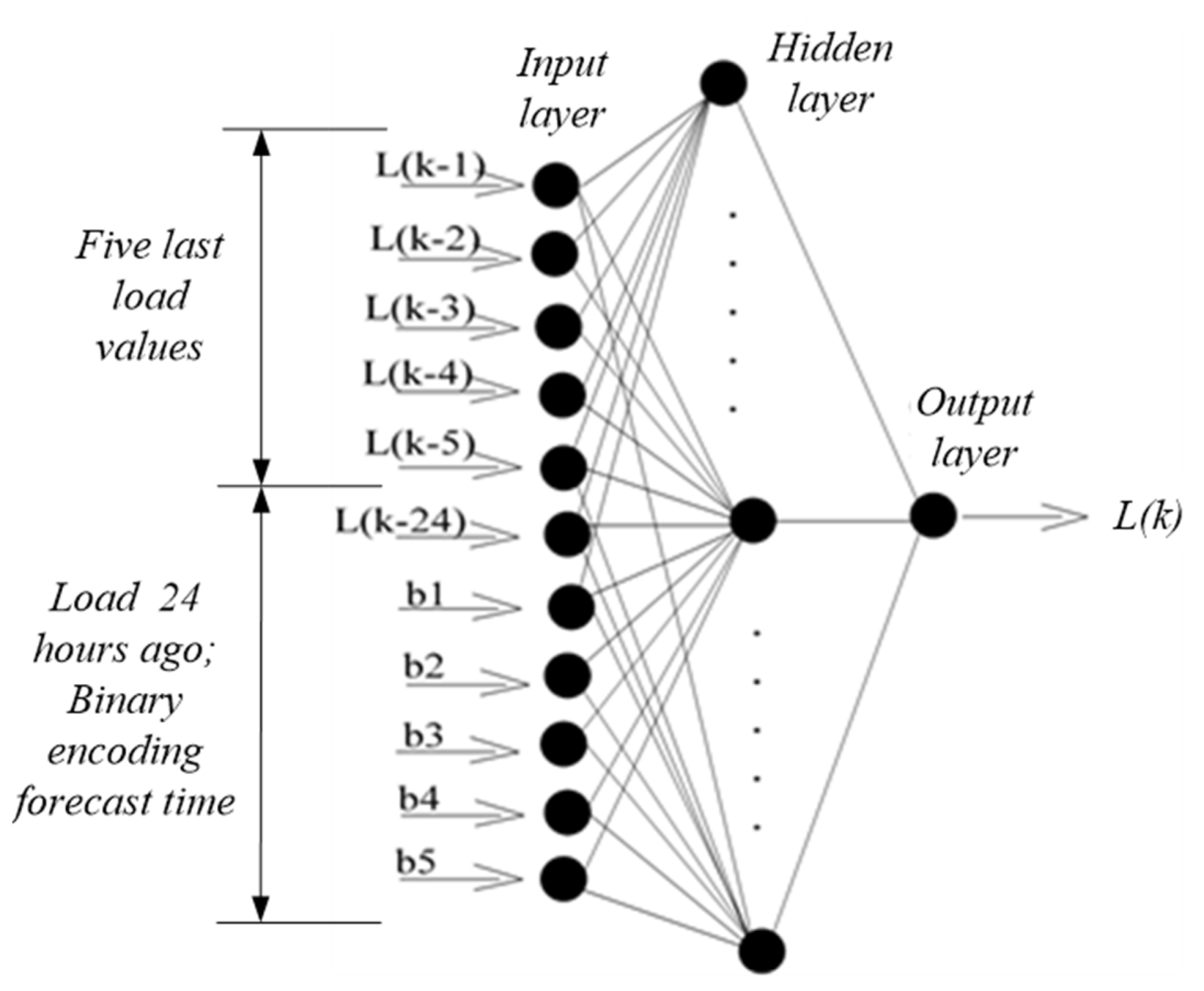
To find the best fit and consequently the best forecasting tool, three ANN models are proposed and compared. In Method I, the forecast hourly load is based on an ANN model using a binary input code for the hour, as used in [
4,
14]. See
Figure 1.
Method II did not use binary encoding. The ANN model used an integer number as an encoding time of an hour (1, …, 24) of the day where it occurred energy consumption. This model used 7 data in the input layer, the same hourly load mentioned in Method I, and added the integer number of the corresponding hour for the last input as an encoding time. The 3rd Method, Method III, completes the latter Method. Using 8 data input, the same hourly load as used in both Methods I and II, the integer number of the hour added the integer number of the day (1—Monday, …, 7—Saturday). Both are used in the input ANN models as an encoding time.
The ANN learning process in this research adopts well-known backpropagation and Levenberg-Marquardt (LM) training algorithms and the activation function hyperbolic tangent sigmoid (HTSF) and pure line (PF) in the hidden and output layers, respectively, performed using the software tool (nntool from MATLAB). Sigmoid and the hyperbolic tangent sigmoid function (HTSF) may lead to saturation of the backpropagation algorithms because of the exponential tendency to grow or lessen the backpropagation of the error signal. In theory, the ReLu activation function, despite being non-differentiable in the origin, can be efficiently retro-propagated, but this may lead to the non-activation of neurons, also called the “Death or Neurons”. In this work, besides PF, the activation function used was HTSF because the output is centred in zero and demonstrates good convergence, despite presenting low convergence and saturation. Further work will exploit other activation functions, such as Leaky ReLU, Maxout, or Softmax. The adaptive moment optimization (Adam) is a replacement optimization algorithm for a classical stochastic gradient descent (SGD) procedure. However, Adam, in some state-of-the-arts results, does not converge to an optimal solution and do not generalize as well as SGD with momentum, which encourages the use of popular optimization algorithms.
The gradient descent is the simplest optimization algorithm. It updates the network parameters in the direction in which the performance function derivate is most negative. Although it does require more memory than other algorithms, the LM algorithm demonstrates faster convergence for networks that contain up to a few hundred weights (as it is for our cases) [
38,
39,
40], as shown in [
16,
18,
37].
The general practice for training the MLP networks starts by dividing the data into three subsets: training, validation, and test sets. The training set is used for computing the gradient and updating the network weights and biases. The validation set measures the model error during the ANN training, which normally decreases. When the network begins to overfit the data, the error on the validation set typically rises. The test set error is independent and is not used during training. The test set is used to compare outputs targets (actual energy load) and the computed values by the ANN. In a typical setup, 70% of the data is used for training, 15% for validation, and 15% for testing.
In this work, the regularization and early stopping methods are used for improving generalization. In the early stopping method, the available data is divided into three subsets, as mentioned above. The other method for improving generalization is called regularization. A performance function frequently used for training feedforward, ANN is the mean square errors (MSE). If predictions deviate too much from actual results, the loss function will increase. Gradually, with the help of the optimization function, the loss function learns to reduce the error in prediction. Using this performance function forces the network to adjust the corresponding weights and biases, and this compels the network response to minimize the performance function. Early stopping and regularization can ensure network generalization when we apply them properly. When we use regularization, it is important to train the network until it reaches convergence. The MSE and the network parameters reach steady values when the network converges.
Validation is a technique for evaluating how the training results will generalize. The purpose of the cross-validation technique is to define a dataset to test the ANN model in the training process, to limit overfitting, and be aware of how the model will be generalized to a new dataset. For early stopping, care must be taken not to use an algorithm that converges too fast.
The learning process is interrupted when the curve corresponding to the validation data decreases to a minimum error value and before it starts to grow in the learning process. In all tests performed and using the validation data subset, it was considered that, if during six consecutive iterations of the learning process the error does not decrease, the learning process is interrupted. By testing several different initial conditions, the network robustness and performance is assessed.
For low-sized datasets, Bayesian regularization (BR) gives better generalization performance than early stopping, because BR does not require that a validation dataset be separate from the training dataset. BR handles the overfitting problem effectively as long as the models are not too complex. The BR approach involves a probability distribution of network weights. As a result, the forecasting of the ANN is also a probability distribution [
41]. Hereby, among the techniques mentioned above and due to inaccuracy performance, the early stopping was used in the training process.
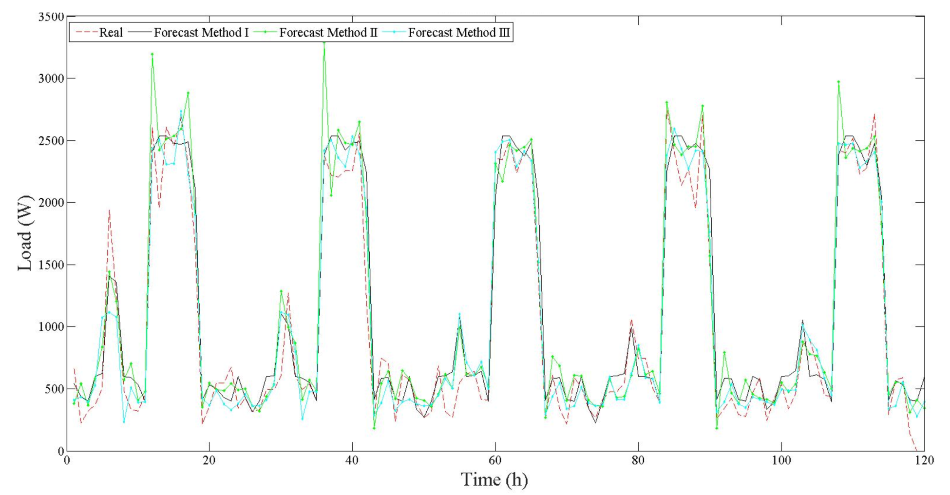
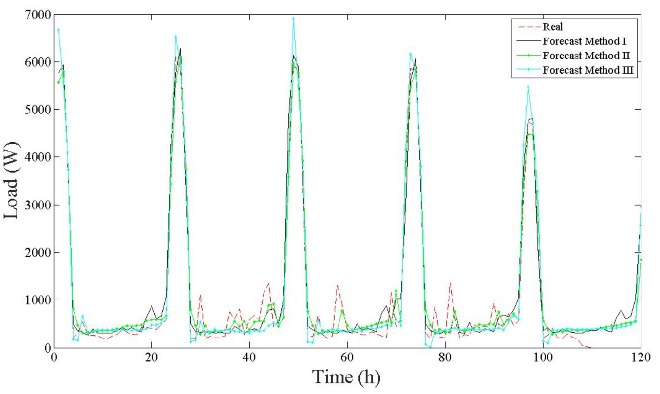
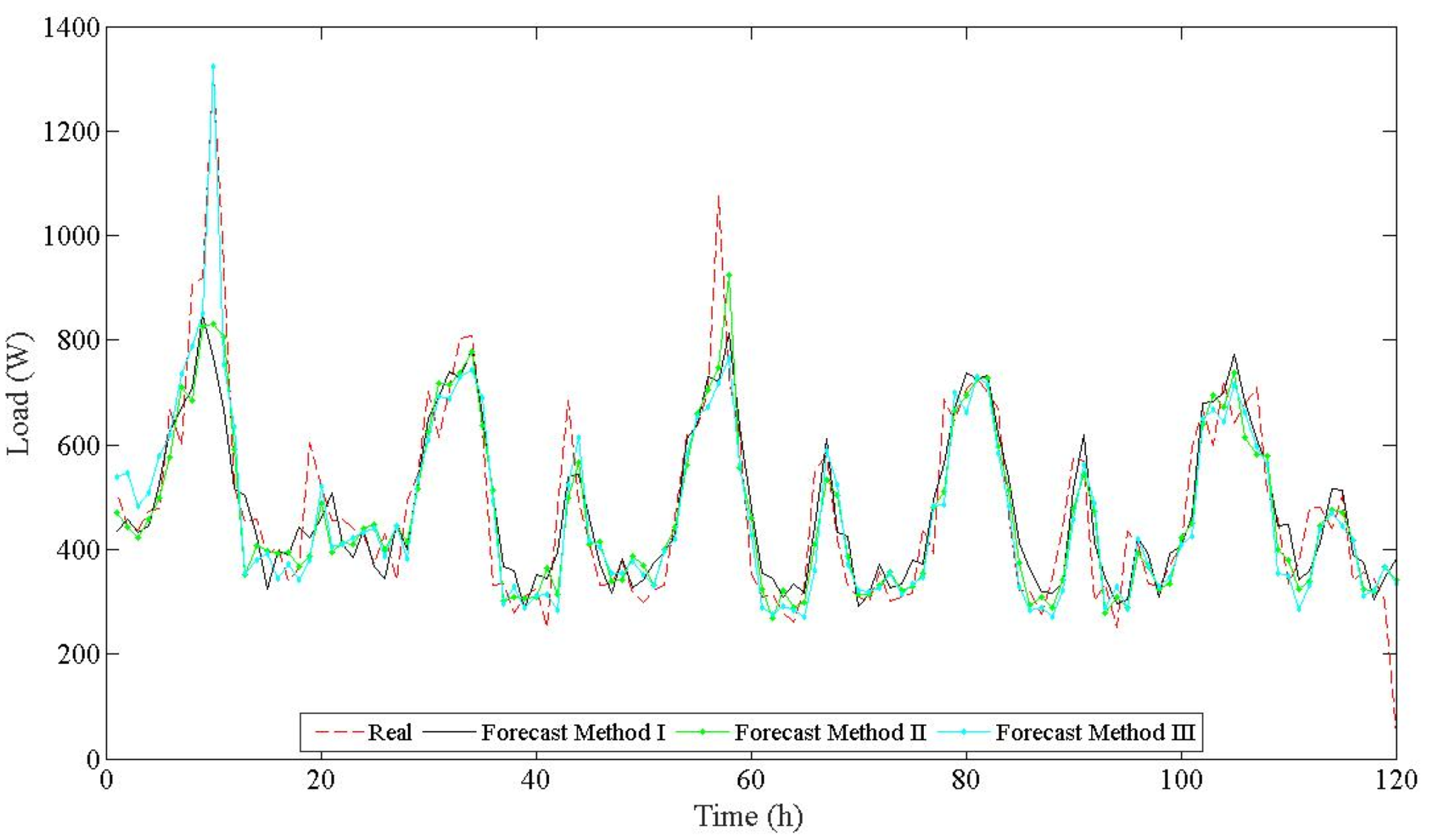
Thereby, the load forecast produced by the ANN can be compared to the actual load data and the error is calculated. Then, the forecasting correlation and error values of outputs are compared with the test set, as well as the shape of the load profile distribution. The effectiveness of this approach is analyzed by forecast outputs results; we will show the performance of the different methods studied in this work.
3.2. Automated Training Process
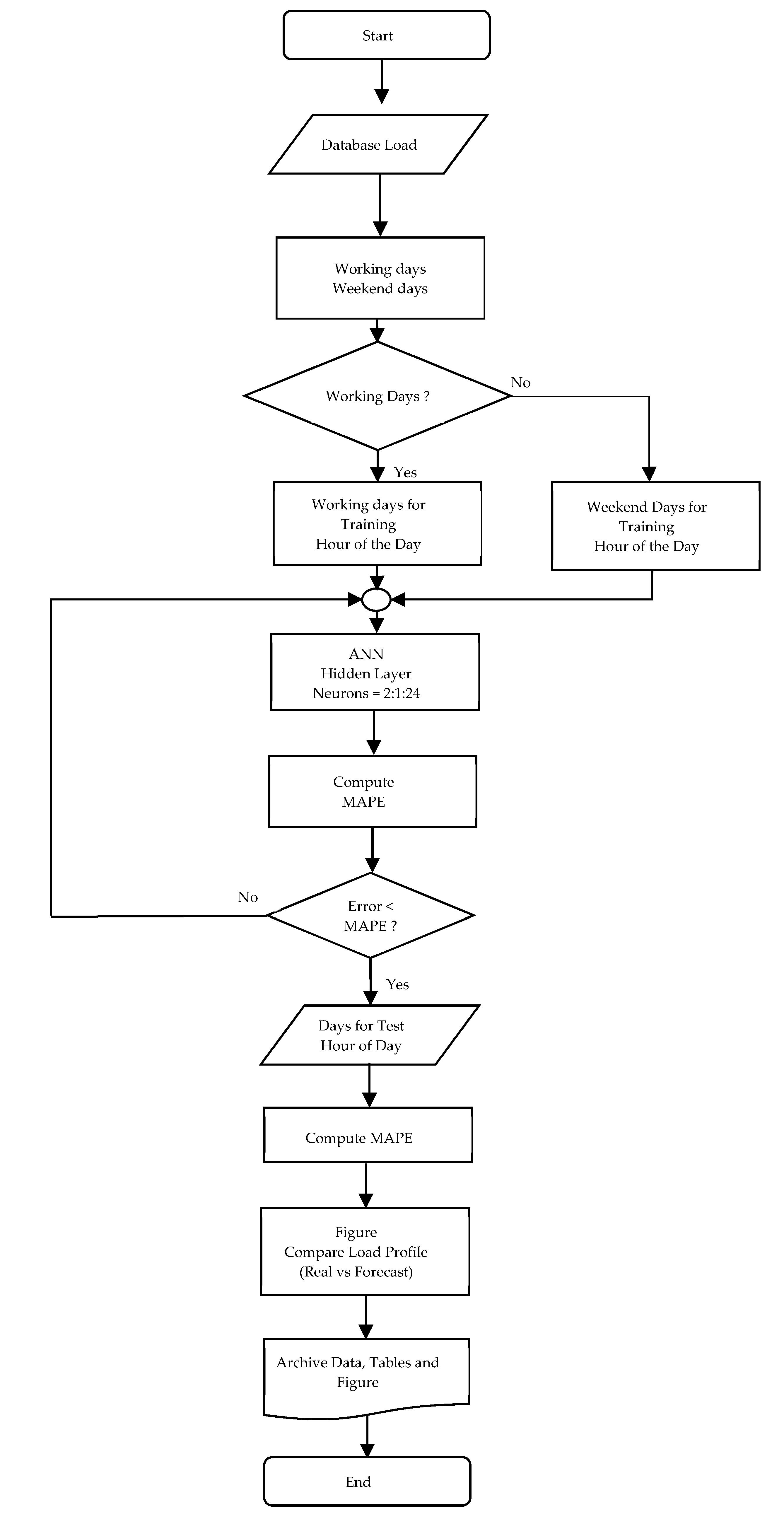
As shown in
Figure 2, to automate the trial and error, a script was developed in MATLAB. This application was able to automatically train the proposed ANN by changing the number of neurons in the hidden layer, after computing the mean absolute percentage error (MAPE), or the mean absolute percentage deviation (MAPD).
The learning process begins by dividing the data from [
16,
18,
37] into 3 subsets, and the LM training method was used with MSE as a performance function. MSE measures the network’s performance and the LM algorithm updates weight and bias values according to the Levenberg-Marquardt optimization algorithm. In many cases, LM can obtain lower MSE than any of the other algorithms tested [
41,
42].
To change the number of neurons in the hidden layer, the used criteria to stop the network training process are as follows:
Minimum gradient magnitude;
Maximum number of cross-validation increases;
Maximum training time;
Minimum performance value;
Maximum number of training epochs (iterations).
During training, the progress is constantly updated in the training window. The most interesting are the gradient magnitude, number of cross-validation checks, and performance value. The magnitude of the gradient and number of cross-validation checks are used to terminate the training process. The gradient becomes smaller as the training achieves a minimum performance value. The number of cross-validation checks represents the number of successive iterations that the validation performance fails to decrease. It has been considered that if this number reaches 6, the training will stop. These limits can be adjusted, and criteria can be changed by setting the parameters. In this research, it was verified that most of the training did stop by the number of cross-validation checks. After the maximum has been reached and the MAPE reach the proposed value, all the learning procedures end. If the proposed value of MAPE is not reached, the neural network will retrain, changing the number of neurons to obtain the best relationships between the actual and forecast load. The neurons’ number changing is performed by an increase of one unit until it reaches the established maximum value. In our case, the minimum value is 2 and the maximum value is 24 neurons.
3.3. Forecasting Performance
MAPE is defined as:
where
LA is the actual hourly load,
LF is the forecasted hourly load,
N is the number of hours, and
i is the hour index.
In the study cases, the standard deviation of errors (SDE) is another criterion used, given by:
where
ei is the forecast error at hour
i and
is the average error of the forecasting period. SDE is just the square root of the MSE. MSE are measures of error that indicate whether the forecasts are biased, i.e., whether they tend to be disproportionately positive or negative. Therefore, minimizing the MSE implicitly minimizes the bias as well as the variance of the errors [
43].
Hourly load consumption may rise or drop at specific hours [
38,
42]. In statistics, the MAPE is a measure of method accuracy for constructing fitted time-series values. It usually expresses accuracy as a percentage and is defined by (2). Hence, the average load was used in (2) to avoid the problem caused by actual loads close to zero. The MAPE is also often used for purposes of reporting because it is expressed in percentage terms, which makes sense for identifying “big” errors [
44].
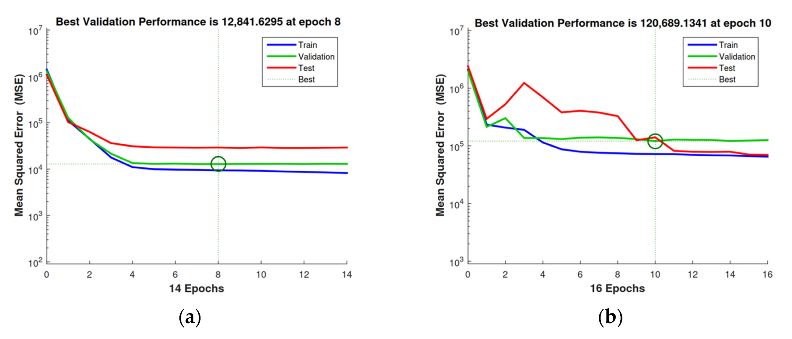
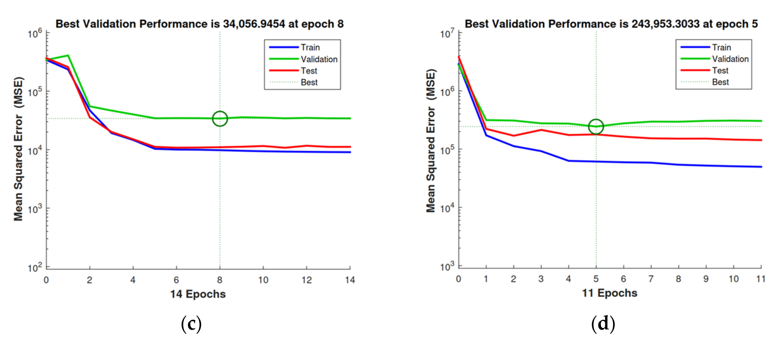
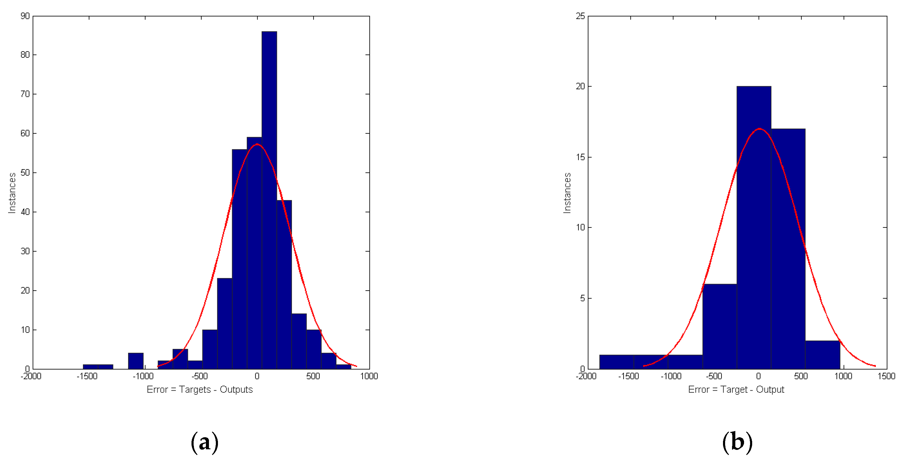
Figure 3 shows the MSE resulting from the training of the energy dataset of a randomly selected household.
MAPE and SDE values for hour-ahead forecasting in different hours of the day are presented in the case studies section. As it can be verified, the MSE starts with high values and, with the training, each epoch tries to reduce the error and stabilize. The MATLAB nntool identifies and marks the best time performance.
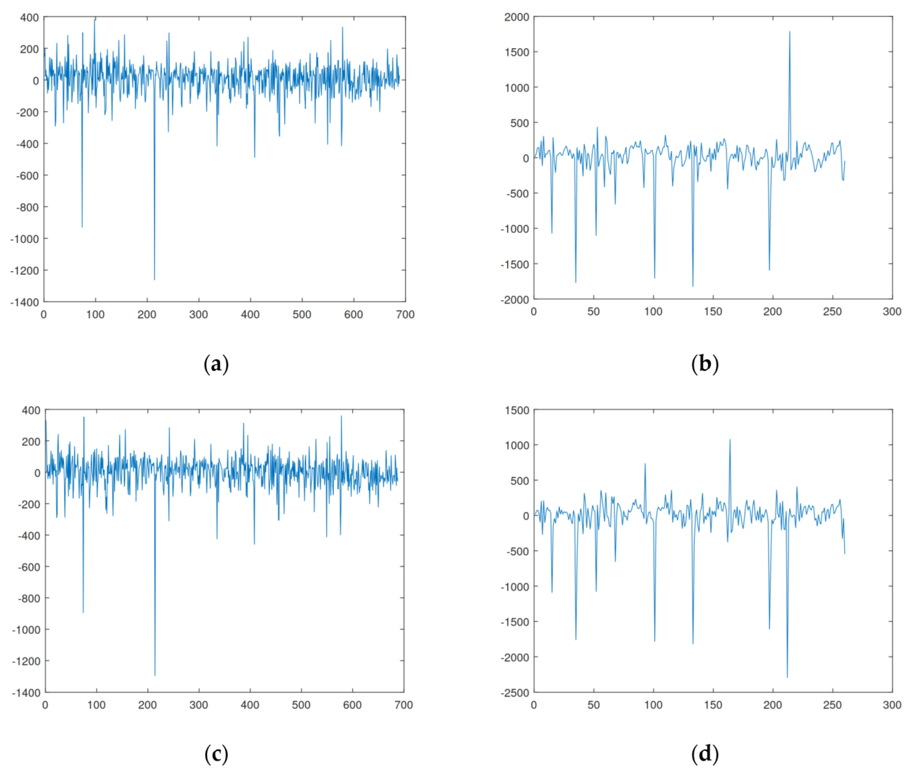
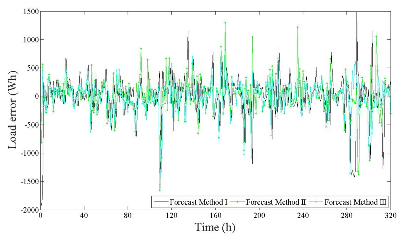
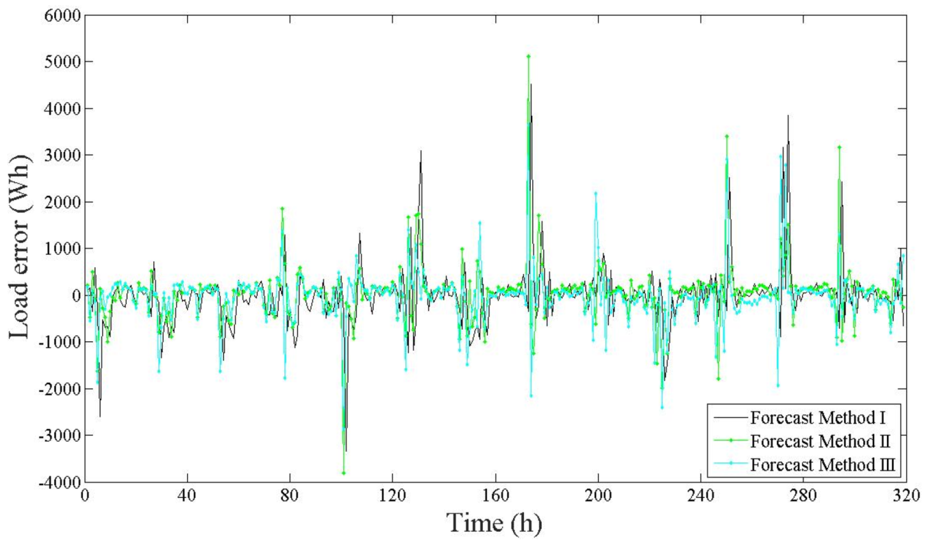
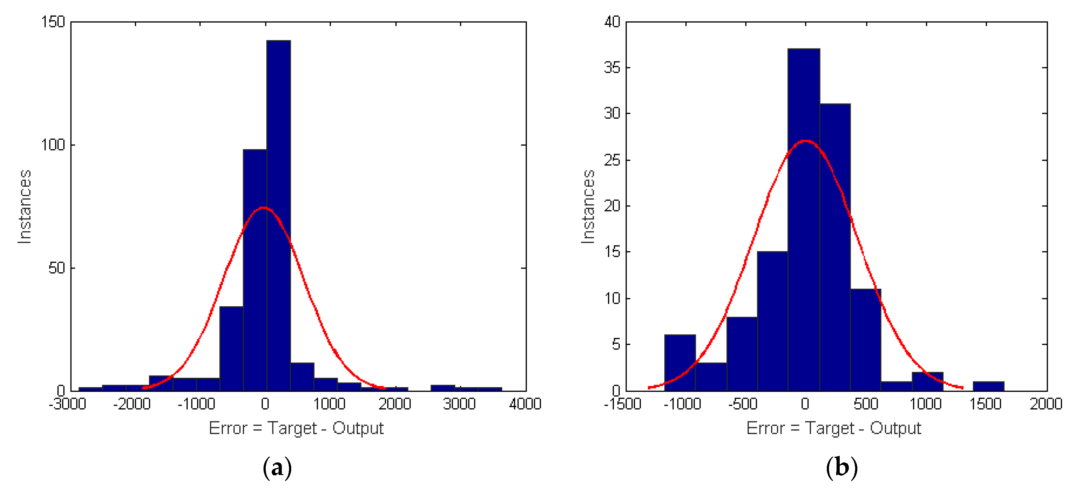
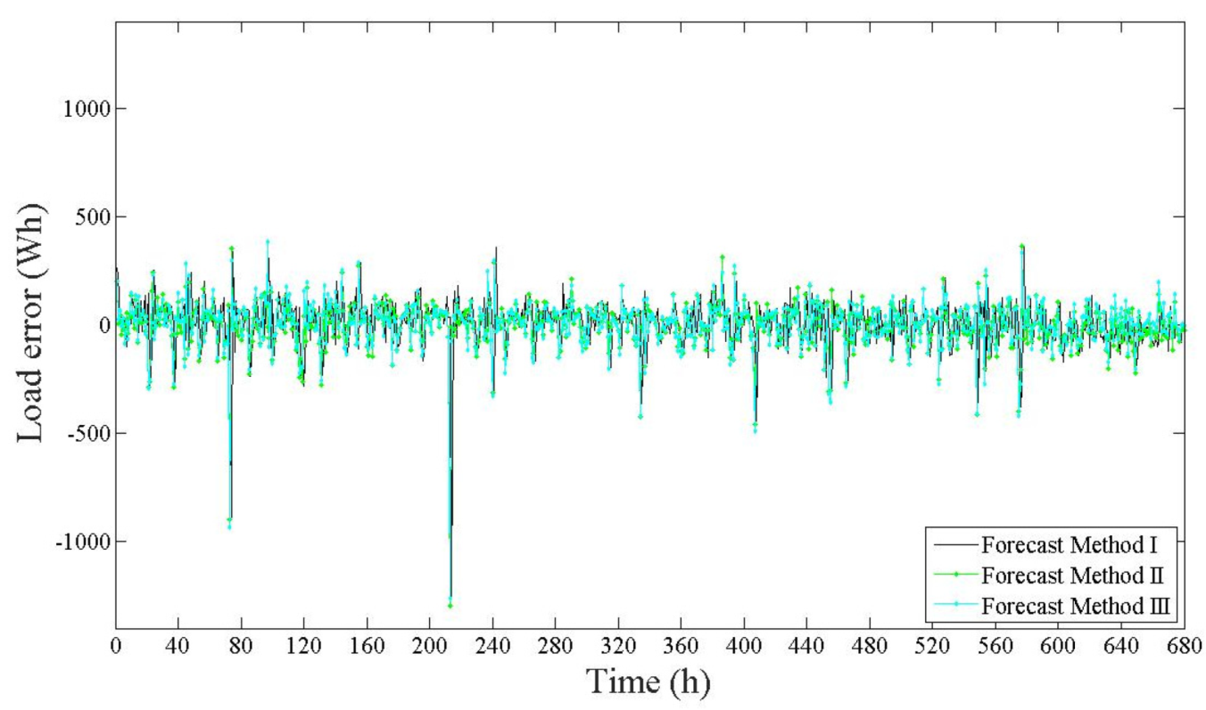
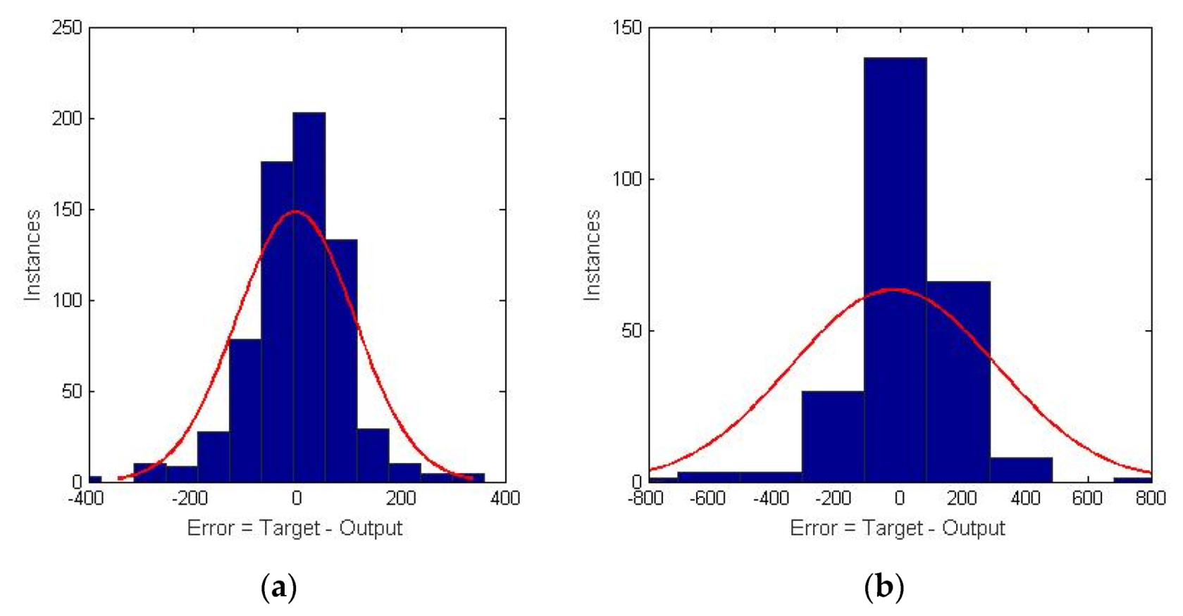
Figure 4 shows the errors resulting from the training.
This study is not a m-class classification problem and does not intend to be a classifier. The receiver operating characteristic (ROC) curves are effective for measuring classifier accuracy in binary-class problems as the f-measure, and for cases of m-class, the kappa statistical metric is applied as a scalar meter of accuracy.


