1. Introduction
The aim of an all-wheel-drive (AWD) system is to optimize maximum driving stability, high-performance agility and good traction in the relevant driving situations (see [
1,
2]). While traction was the main focus of AWD systems in the early years, aspects of driving dynamics also increasingly came to the fore in the later years of development [
3]. Both automatically switchable AWD systems (e.g., 4MATIC [
4]) and controlled permanent all-wheel-drives with fully variable torque distribution (e.g., Porsche 959 [
2]) offered new possibilities for influencing driving behaviour from the very beginning of AWD development. The introduction of electronically controlled all-wheel-drive systems has made it possible to adapt the drive torque distribution by a control unit. With the option of using sensor signals in the mechatronic system, the driving dynamics can be influenced by an AWD system depending on the driving situation. As sensor technology has continuously developed, further important information for all-wheel-drive systems has become increasingly accessible. Newer approaches have recently made it possible to obtain more precise knowledge about the tyre–road conditions, beyond the adhesion limit of the tyres. Especially road wetness is an important information.
It is known that all-wheel-drive systems develop a great driving dynamic effect especially when their actuating wheel forces come close to the adhesion limit, see [
5]. Thus, the maximum frictional potential of the tyre–road contact plays an important role. In the case of chassis control systems in particular, which have their effective range in the area of the frictional potential limit, an adaptation to the adhesion limit is particularly advantageous, see [
6,
7] for instance. In addition to the sole value of the adhesion limit, however, it is also important to gain knowledge of the condition of the road, such as snow, rain or ice. In particular, the presence of an intermediate medium such as water not only requires an adaptation of the assumed friction coefficient of an all-wheel-drive system. It is also necessary to adapt the driving dynamics targets. Depending on the driving situation, wetness can quickly endanger driving stability (see the tyre force transfer properties under wet conditions in [
3,
8]). Driving on wet pavement requires an adaptation of the driving behaviour towards more driving stability.
On the other hand, it becomes clear that the increasing diversity of vehicle variants (see variety of models and complexity in [
9]) in combination with further new specific driving programs result in a time-consuming calibration of the chassis control systems. As a result, it is necessary when introducing new control strategies, such as the integration of wetness information presented here, to generate as little additional calibration effort as possible. With this goal in mind, this work should make a helpful contribution to innovative all-wheel-drive controls by introducing a significant model-based expansion of wet functionality using just a few parameters - without multiplying calibration efforts.
1.1. State of the Art—Estimation of Tyre-Road Conditions
The observation of the tyre–road conditions is still a topical issue today. Especially estimating the friction coefficient itself has been the subject of research for decades. For this reason there are numerous works that substantiate the research activities [
10,
11,
12,
13,
14]. In one of the early patent applications [
10] a method was derived for determining the adhesion and adhesion limit for vehicle tyres. The inventors use a driving dynamics simulation model in which tyre characteristics are adapted to the current tyre behaviour of the real vehicle. Within all research projects, one major challenge is the on-line identification of the friction coefficient. To this subject the studies [
11,
12] make a significant contribution. In [
11] the authors present a slip-based method for tyre–road friction estimation with higher robustness compared to previous studies. Over and above that, the thesis [
12] presents an estimator of the friction potential which is solely based on measurements of the driving dynamics of the vehicle. An observer has been developed for this purpose. It is used to calculate the internal state variables required to estimate the friction coefficient during driving. Apart from the established, conventional estimation approaches, the latest studies use machine learning algorithms to determine the tyre–road friction coefficient [
13,
14].
In addition to the pure estimation of the adhesion limit, there are also investigations with the aim of detecting the condition of the road surface and, in particular, wetness [
15,
16,
17,
18,
19]. The early patent application [
16] proposes the measurement of the splashing water noise or the rolling noise of a wheel by a sensor attached to the vehicle. The research in [
15] elaborates the observation of the road condition. The approach presented enables the detection of dry, wet, snow-covered and ice-covered roads. A combination of software, algorithms and external electronical sources (such as cameras) is used to classify the road condition. As an outlook, the study highlights the importance for advanced driver assistance systems (ADAS). The study [
17] is devoted to classify of the friction coefficient also differentiating between dry and wet conditions. In addition to the vehicle sensors the method requires data from at least one weather station and one ice warning system. In [
18] a real-time acoustic analysis of tyre/road noise is presented in order to get a wet/dry classification of the road surface. This method is finally expanded in [
19] to a wider range of road conditions.With the new generation of the Porsche 911, a system for detecting road wetness was introduced in series production [
20]. In this case, an acoustic sensor in the wheel arch of the front axle detects the intensity of the water spray. As soon as the sensors reliably detect road wetness, the driver receives a message in the instrument cluster.
1.2. State of the Art—Adaptation of Chassis Control Systems to Tyre-Road Sonditions
Assuming that information about the tyre–road condition is available, the question arises as to how mechatronic chassis control systems can best benefit from the information. Several approaches for the adaptation of chassis control systems in general to these conditions have been investigated to date—also outside of all-wheel-drive systems [
6,
7]. The research in [
6] examines the benefit of sensor information about the friction coefficient for an anti-lock braking system (ABS)—available before the start of control interventions, for an electronic stability program (ESP) and for an active front steering system (AFS). In [
7] a number of influencing variables on the transmission of tyre forces are examined first. In the second step—in the simulation part—the peak grip potential is used for an adaptive tyre model in order to increase the maximum lateral performance by means of a torque vectoring control system. Otherwise no distinction is made between dry and wet roads.
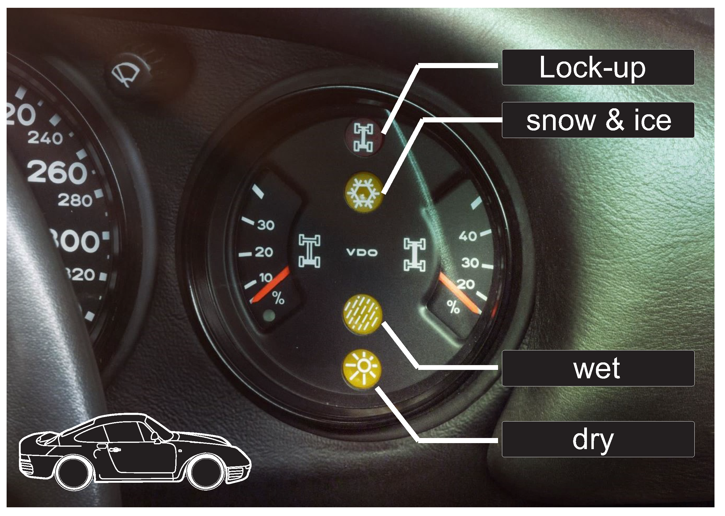
An adaptation to the tyre–road condition was also implemented for all-wheel-drive systems. In the mid-1980s, when AWD development was making great leaps, the first attempts were made to adapt an AWD system to the traction conditions. The endeavor to adapt important chassis control systems to the traction conditions can already be seen using the example of the Porsche 959 super sports car. The driver was able to choose between following different programs for the all-wheel-drive control: dry, wet, snow and ice and a lock-up mode, see [
2]. The driving mode selected by the driver was displayed in the instrument cluster with a control lamp (see
Figure 1). Even if at that time there was no sensor detection to recognize the road condition, the need to design a separately adapted all-wheel-drive control was taken into account. The latest generation of the Porsche 911 also has a special driving mode for wet conditions that can be selected manually using a driving mode switch. When selected, several mechatronic systems (ABS, adaptive aerodynamics) are adapted, including all-wheel drive [
20,
21]. The preconfiguration of the AWD is given by a basic torque distribution which biased to the front [
21].
Nevertheless, providing new, specially adapted driving modes is associated with not inconsiderable additional effort in development and calibration. In the previously known approaches from the literature, it has not yet been sufficiently worked out how to arrive at a comprehensive AWD control strategy that not only allows a functional expansion to include wetness information, but also takes various degrees of wetness into account.
1.3. Concept of This Work
This work presents a concept to beneficially use information about road wetness in an all-wheel-drive control. The tyre friction estimation and the road condition observation are not part of this study. Rather, the study serves to work out the potential for an AWD system, assuming the friction coefficient and the road condition (here in form of road wetness) are known. For the wetness information, it is assumed that different degrees of wetness can be distinguished, since acoustic or acceleration sensors can determine qualitative gradations of the water intensity on the street, see [
20,
22]. In this work the “degree of wetness“ is used in a generic way as a quantitative indicator of various levels of wetness without knowing the exact water film height.
The starting point for the concept is the United States Patent Application Publication “Method for distributing a requested torque“, see [
23]. In a generic way it describes a model-based approach for an all-wheel-drive system in order to distribute drive forces between two drive axles. One advantage of the concept presented in [
23] is the fact that calculation of the drive torque distribution is based on the current utilization of the friction coefficient on one drive axle. This utilization is continuously calculated in order to distribute the torque requested by the driver to the second drive axle. The minimum torque distribution is carried out using a distribution key that is not further specified in [
23].
The aim of this work is to expand the all-wheel-drive control concept mentioned in [
23] so that available information about occurring road wetness can be implemented profitably. In particular, the method is to be expanded in such a way that not only the assumed friction coefficient in the controller is adapted, but also the driving dynamics targets are to be adjusted. In this approach the advantages of a model-based control should be retained as well as the possibility of applying a favorable all-wheel-drive torque distribution using just a few physical parameters. The method is applied to a vehicle with a torque-on-demand transfer case and is evaluated by full-vehicle model simulation.
2. Topology of the All-Wheel-Drive with Torque-on-Demand Transfer Case
The topology of the all-wheel-drive vehicle with a torque-on-demand transfer case is presented below. It shows the power flow during the force transmission and will serve as the basis for the derived concept of an adaptive all-wheel-drive control. In the following, a quasi-stationary driving condition is assumed and all power transmission elements in the drive train are assumed to be torsionally rigid and massless.
Schematic Overview—Kinematics and Torques
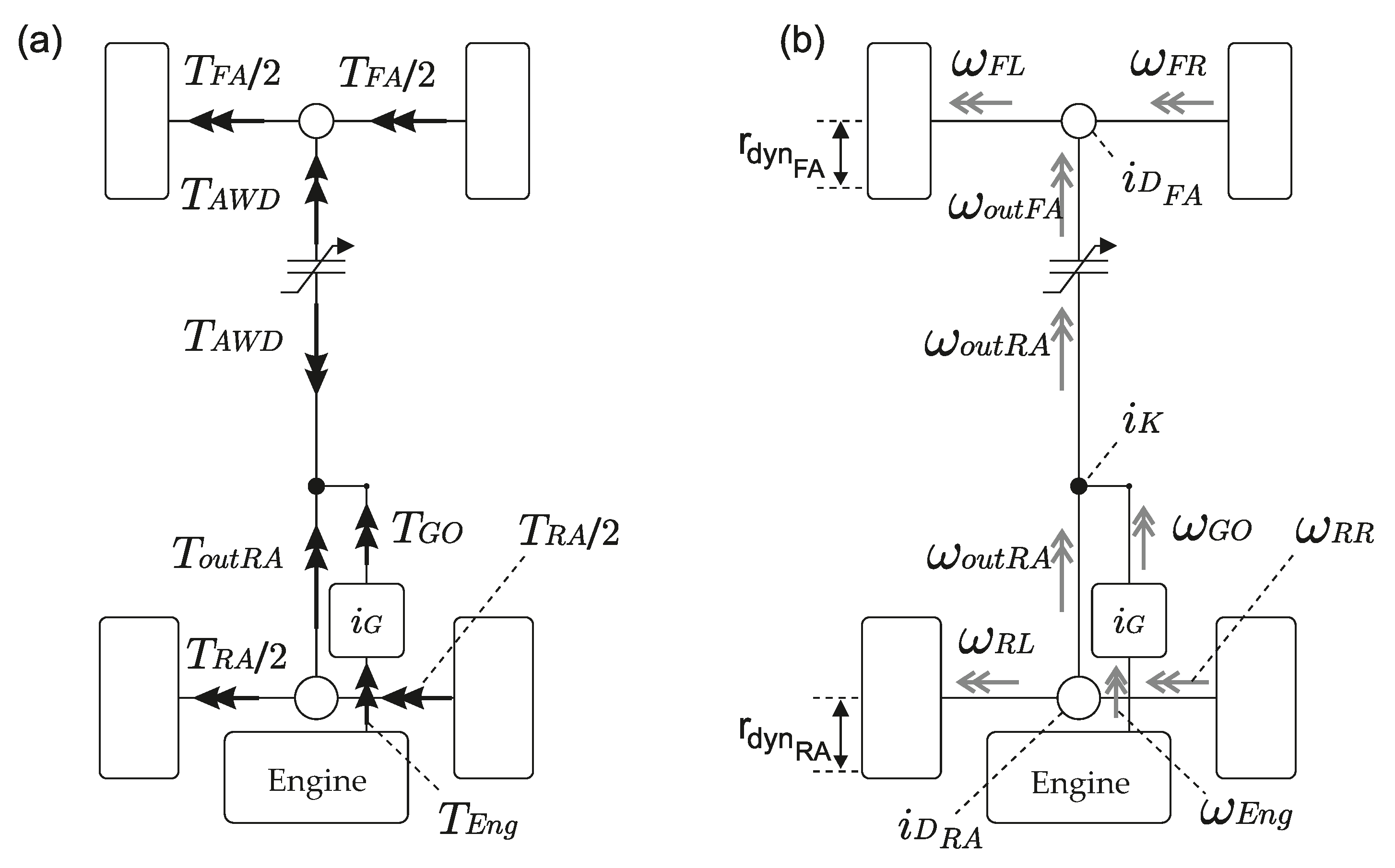
Figure 2 shows (a) the torque flow from the engine to the drive axles and (b) the rotational speeds along the entire powertrain. The meani g of the abbreviations are listed in
Table A1. When the clutch is engaged the engine torque
and the engine speed
are transmitted by the main gearbox with the gearbox ratio
to the output torque
and to the output rotational speed
. A constant gear stage
finally leads to the main drive shaft, which rotates with the rotational speed
. The rotational speed of the main drive shaft
serves as the input speed for the rear axle differential and as the input speed for the all-wheel-drive clutch at the same time. The rear axle differential is used to compensate the speeds between the left and the right wheel. Thereby, the input rotational speed of the differential
is transmitted by its ratio
into an average rotational speed
of the rear axle (see the modeling of a differential gear in [
24]). This equation is listed in
Table 1 together with all the following equations for speeds and torques.
Concerning the force transmission on the main drive shaft different torque values occur in direction of the front and in direction of the rear axle. The total input torque to the main drive shaft transmitted by the constant stage is divided into two parts, a first part to the rear axle and a second part to the front axle , which is applied to the all-wheel-drive clutch. The drive shaft torque to the rear axle serves as the input torque for the rear axle differential. If the self-locking effect in the differential is neglected and there is no active differential locking torque, the rear axle differential with the ratio converts this input torque into two equal torques .
The torque-on-demand transfer case transmits the applied clutch torque
to the input side of the front axle differential, which is rotating with
. The front axle differential then converts this input speed
with its gear ratio
into an average drive speed
of the front axle wheels. The power loss
occurring at the torque-on-demand transfer case can be calculated as follows:
3. Driving Dynamics Targets for All-Wheel-Drive Control in Wet Conditions
The adaptive all-wheel-drive control developed in the following is intended to increase the coverage between the desired driving performance on dry roads and the necessary driving safety in wet conditions. This is done by the control, taking into account information available about the presence of wetness and using it beneficially. In summary, the primary requirements for the adaptive all-wheel-drive control when wetness information is available are:
stability:
- −
increase in vehicle stability and avoidance of oversteer situations by influencing the vehicle balance with combined dynamics;
- −
implementation of a suitable basic torque distribution in pull operation with partial throttle actuation and higher accelerator pedal positions; and
traction:
- −
increasing the longitudinal acceleration capability of the vehicle.
On the other hand, there are some requirements that are of secondary importance to traction and stability, especially under wet conditions; but, they must be taken into account permanently as important boundary conditions for the adaptive all-wheel-drive control. The secondary requirements are:
4. Control Strategy in Dry and Wet Conditions
The control strategy of the adaptive all-wheel-drive is developed below. As a central task, the control may beneficially use the information about road wetness. The starting point for the adaptive control strategy of the all-wheel-drive is the
“Method for distributing a desired torque“ described in [
25]. This method calculates the distribution of the drive torque on both axles of an all-wheel-drive vehicle on the basis of the driver’s request, i.e., using the accelerator pedal position
.
4.1. Control Strategy without Specific Implementation of Wetness Information
The overriding goal of the control strategy described in [
25] is not to exceed the grip limits of the two drive axles and only to use the available longitudinal friction potential of the tyres for the drive force distribution. Within the adhesion limits of both drive axes, the drive torque is divided depending on an adjustable parameter
, still to be defined. The control strategy in [
25] is largely based on the calculations summarized in
Table 2.
The equations are used to estimate individual wheel forces and their used and remaining friction potentials, respectively. A quasistatic driving condition is assumed for all calculations. The equations are divided into individual modules according to their physical meaning and are explained in more detail below.
4.1.1. Maximum Global Friction Limit
The currently existing adhesion limit
between the tyre and road surface serves as one basic parameter for distributing the requested drive torque. The information can be provided by estimation of the friction coefficient. In this work it is assumed that the current nominal friction coefficient
is known from current methods from the state of the art, see
Section 1.1. Starting from this nominal value, the adhesion limit for each tyre decreases with increasing wheel load and is, therefore, dependent on the driving situation. Therefore, based on the nominal friction coefficient
, a wheel load-dependent adhesion limit
is calculated for each wheel, which takes into account the degression of the friction coefficient:
The parameter
describes the degression of friction coefficient and the normalised change in vertical load
is calculated by
4.1.2. Wheel Loads
The wheel loads
are estimated using a simplified twin-track model. Dynamic wheel load transfers are superimposed on the static wheel loads
. The wheel load transfers are proportional to the longitudinal and lateral acceleration
of the vehicle. The constant of proportionality in longitudinal direction is called
. Its value depends on the height of the center of gravity
, the wheelbase
l and the vehicle mass
m. The constant
for the lateral direction mainly depends on the spring stiffness, damping rate, roll center height and the roll torque distribution determined by the anti-roll bars (see [
26]).
4.1.3. Wheel Sideforces
The wheel sideforces
are estimated by allocating the inertial force
to the two axles according to the center of gravity. In a second step, the sideforce
is divided between the left and right wheels. In the the original approach in [
25] the distribution is linear based on the wheel loads
. It applies if one assumes that the tyre lateral force increases linearly with the wheel load at a given slip angle. However, it should be noted that the linear distribution of the sideforces according to the wheel loads is not precise. It is a first approximation for low-wheel-load transfers. With higher wheel loads, the friction potential of a tyre decreases. As a result, the tyre can no longer transfer sideforces in a linear proportion to its wheel load. A higher accuracy can be obtained if one knows the degressive sideforce characteristics of the tyres more precisely. For the developed control in this paper, the lateral force calculation will therefore be expanded. Departing from a linear allocation of the sideforces in [
25] the wheel load degression of the friction potential is taken into account. The forces are, thus, not divided according to the ratio of the wheel loads, but according to the ratio of the maximum tyre force potential:
4.1.4. Used Friction Potential
The used friction potential
is a parameter that indicates the percentage of the maximum friction coefficient
that is being used by the wheel forces. Thus, in order to calculate
, the wheel forces
,
and wheel loads
must be known. If one relates the occurring wheel forces
or
to the wheel load
, one gets the actually used friction coefficient
or
respectively. Normalizing
or
to the maximum friction coefficient
, finally leads to the used friction potential
and
respectively (see
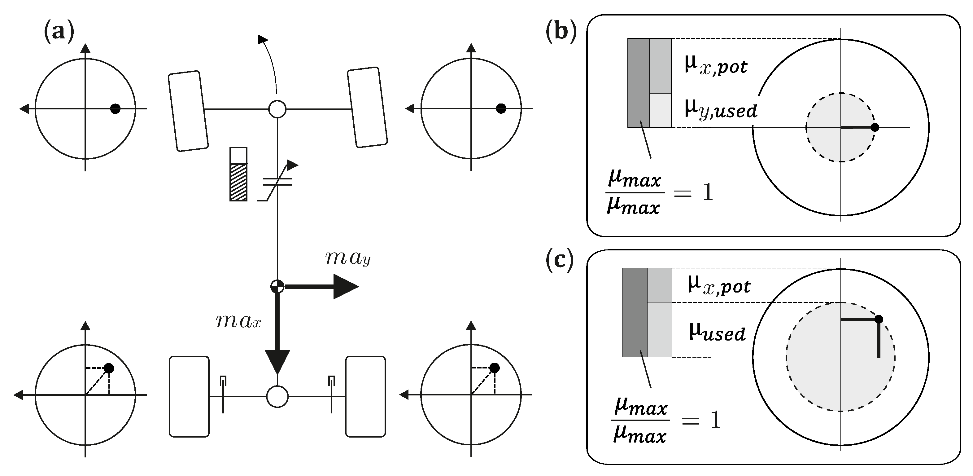
Table 2). The global used friction potential
of the combined wheel forces on a tyre is geometrically composed of the two components
and
(see
Figure 3c).
4.1.5. Remaining Friction Potential and Available Traction Force on Front Axle
The used friction potential
is utilised to calculate the remaining friction potential
on both drive axles (see
Figure 3b,c and
Table 2). On the front axle, the value for the remaining friction potential
determines the maximum possible all-wheel-drive force. The all-wheel-drive force limit is reached if the resulting tyre force—consisting of the all-wheel-drive force and the tyre sideforce—exceeds the tyre adhesion limit. To do this, the remaining friction potential
and, thus, the available traction force
is determined from the geometric distance between the resulting tyre force vector composed of
and
and the friction circle of
Kamm. The available traction force
on each of the two front axle tyres then results in:
The available traction force
on the front and rear axle is finally defined as follows:
4.1.6. Calculation of the Front and Rear Axle Drive Force
The adjustable parameter
on which the drive torque distribution depends can be defined in various ways. According to [
25], the definition of the parameter
can be based on, for example, efficiency criteria, stability criteria, or criteria relating to the tyre friction limit. In the latter case, the parameter
may be determined by the ratio of the currently applied drive force
on both rear axle tyres to the total available rear axle traction force
. The parameter
thus describes to what extent the available traction force
on the rear axle is used in the current driving state:
In the following, the value of this parameter
is used as the
distribution key for the all-wheel-drive torque. Within the available front axle traction force
it defines the amout of all-wheel-drive torque to be transferred to the front axle. The front axle drive force
is the product of the available longitudinal force
on the front axle and the distribution key
:
The more the longitudinal traction force potential of the rear axle is used (increasing values for ), the more the available longitudinal force on the front axle is also used by the all-wheel-drive system.
4.2. Implementation of a Wetness Information into the Control Strategy
The presented all-wheel-drive control principle according to [
25] generally uses the information about the maximum global friction coefficient
, regardless of whether wetness occurs. In the following, the approach presented is to be expanded in particular for the implementation of wetness information. Thereby, a few and at the same time physically clear parameters are to be created for the implementation of a wet calibration.
The aim is to achieve the driving dynamics goals derived in
Section 3 under wet conditions. If there is no road wetness or if the driving state is sufficiently far from the vehicle dynamic limits, the all-wheel-drive should continue to primarily take agility and efficiency criteria into account in its torque distribution.
4.2.1. Overview—Wetness Coordination Unit
A wetness coordination unit is introduced to adapt the drive torque distribution to occurring wetness on the road.
Figure 4 shows an overview of the overall concept. The starting point is an extended all-wheel-drive control to which a wetness coordination unit is superordinate. If there is a risk of wetness, the wetness coordination unit coordinates the optimal torque distribution through various interventions in the all-wheel-drive control. The basic structure of the the AWD control strategy is presented in the lower part of
Figure 4. It is based on the already introduced basic equations (see
Table 2) according to [
25].
The calculation is clustered in the following three modules: the wheel force calculation, the determination of the used and remaining friction potentials, as well as the determination of the drive torque distribution. The final goal of the calculation is to get a target value for the front axle drive force , using an extended distribution key which is presented later. The interventions by the wetness coordination unit are presented in more detail below.
4.2.2. Modification of the Remaining Friction Potential on the Front Axle
The parameter
is a new, physically based calibration parameter that defines the proportion of the already used lateral friction potential
of the front axle that should remain undisturbed by a longitudinal force of the AWD:
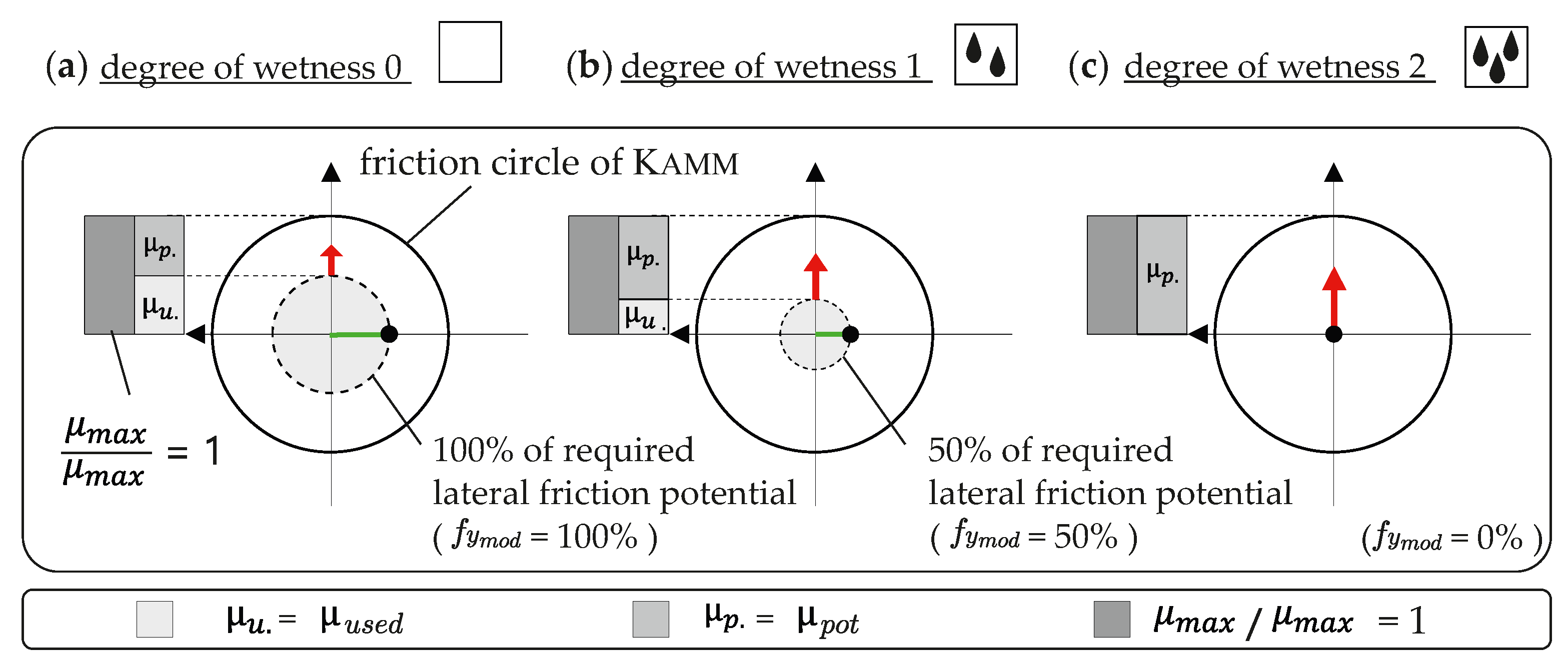
Figure 5 is basically there to illustrate the effects of an increasing parameter
within the all-wheel-drive calculation. A friction circle of
Kamm with an adhesion maximum
is shown in each case (a–c). The friction circle is normalised, however, so that there is a circle radius of
—as in
Figure 3. At the same time, the lateral force required for cornering and, thus, the required used lateral friction potential
is drawn in each subfigure (a–c). If
, then the full sideforce is also taken into account in the calculation of the the remaining friction potential
. On dry conditions the parameter
is set to one. Thus Equation (
8) corresponds exactly to the calculation of the remaining friction potential
in
Table 2. That means, the used lateral friction potential
required to maintain the lateral acceleration of the vehicle will not be affected, illustrated in
Figure 5a. When wetness is detected, the lateral friction potential
on front axle that is needed for cornering is only partially taken into account and more friction potential
is made available for the longitudinal force (see
Figure 5b,c). This is intended to increase vehicle traction on wet conditions by making more longitudinal force potential available within the friction circle of
Kamm. The degree of wetness with which
is reduced can be defined continuously or in discrete steps.
In the following, two other degrees of wetness are defined in addition to the dry road surface: medium wetness (1) and intensive wetness (2). At degree of wetness 1, see
Figure 5b, the parameter
is reduced to
. Finally,
Figure 5c illustrates the situation for degree of wetness 2. With
the entire friction potential of the front axle tyres is made available for traction forces. The developed concept (Equation (
8)) thus represents a computational construct in order to give the application of drive forces a higher priority than the lateral forces that would be necessary to maintain the current lateral acceleration. As a result, higher slip angles will occur on the front axle and the vehicle will lose agility, but in favor of greater use of the traction potential and in favor of vehicle stability.
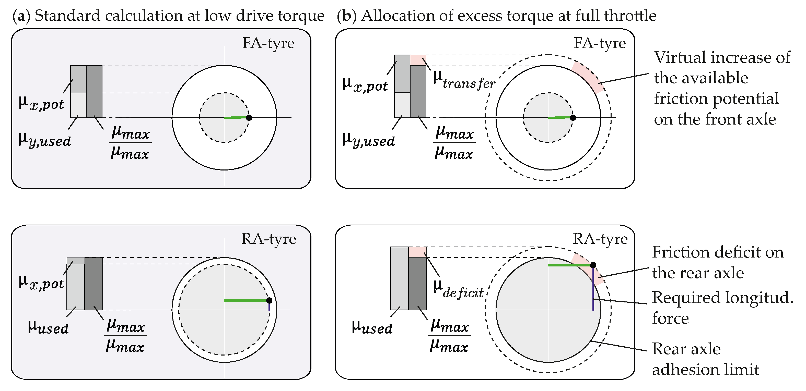
4.2.3. Special Function—Friction Coefficient Transfer in the Event of Excess Torque
For the calculation of the remaining friction potential
on the front axle (see Equation (
8)), an additional special function is introduced, which only intervenes when high driving forces are required from the driver. Looking at the previous calculation of the used friction potential
, it is clear that it was previously assumed that the requested drive torque does not exceed the friction limit
of the rear axle tyres. The friction coefficients for this common driving situation have already been shown as an example for a front axle and a rear axle tyre in
Figure 3. This situation is taken up again in
Figure 6a. The resulting tyre force vector of the rear axle tyres—composed of
and
—remains within the friction circle of
Kamm. Thus a longitudinal force potential
is still available on the rear axle tyres.
If a high drive torque is requested at the same lateral acceleration, the resulting tyre force—composed of
and
—arithmetically exceeds the friction limit
at the rear axle, see
Figure 6b. As long as there is an open differential, the exceeding will preferably occur first on the unloaded wheel on the inside of the corner. As a result, there is no remaining longitudinal friction potential
, but there is a friction deficit
on the rear axle as shown in
Figure 6b for this wheel.
From the friction deficit
, an equivalent of excess drive force
and from this a mean drive force excess
on the rear axle is calculated:
Instead of bringing the rear axle tyre into full sliding due to the high torque requirement, the special function is intended to transfer a large part of the driving force excess
to the front axle in order to further stabilize the vehicle. Alternatively, the engine torque could also be reduced in the same way as an traction control intervention operates, but this would impact the longitudinal acceleration that can be achieved by the vehicle. The special function, on the other hand, ensures that the driver’s request for more drive torque can also be implemented on snow, ice or gravel, for example. In order to remain consistent with the previous model-based all-wheel control, a traction potential
to be transferred is calculated from the pre-calculated excess drive force
of the rear axle, by which the maximum traction potential
is increased virtually at the front axle (see
Figure 6b and Equation (
12)). In this way, the front axle tyres have virtually more traction potential available.
4.2.4. AWD Distribution Key
The original AWD control strategy without implementation of wetness information was described in
Section 4.1. It uses the parameter
to determine the basic AWD torque distribution of the vehicle. In the following a modified distribution key
will be introduced. Therein, the original distribution key
is intended to be weighted by the wetness coordination unit as a function of the occurring wetness level. In this way, the calculation of the front axle drive force
(Equation (
7)) changes into the following equation:
For this purpose, a self-map is introduced by
, which maps
into the same value range
:
The self-map (
14) should fulfill two properties. First, the function
should increase monotonically and second,
should meet the function values
, i.e., with vanishing longitudinal forces on the rear axle (
), no AWD torque is applied to the front axle. Furthermore, when the torque requested by the driver is so high that the longitudinal friction potential of the rear axle is used to the maximum (
), the full remaining longitudinal friction potential of the front axle should be used. The design of the self-map function (
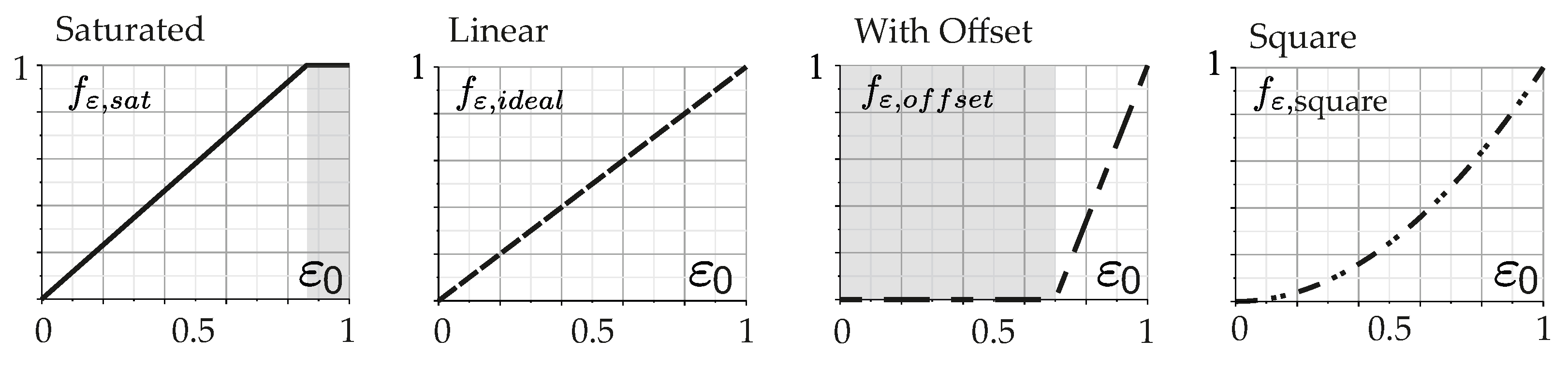
14) offers new options for coordinating a base torque distribution in wet conditions. The following shows four examples for the function course of a
modified distribution key (visualised in
Figure 7). In the first two examples,
is strictly increasing:
It is also possible to define the monotonically increasing but not strictly increasing function
. In this case, the functional value
remains constant in sections of the definition range of
:
With the function the function value is saturated to one before reaching the maximum longitudinal force potential at the rear axle. The function , on the other hand, offers an offset range in which no AWD torque is provided. Thus, with low drive forces, this corresponds to a vehicle with pure rear-wheel-drive. The characteristic is particularly advantageous if, for reasons of efficiency or for reasons of component protection, it is not desired to operate the all-wheel-drive with low drive forces.
5. Assessment Criteria and Test Manoeuvers
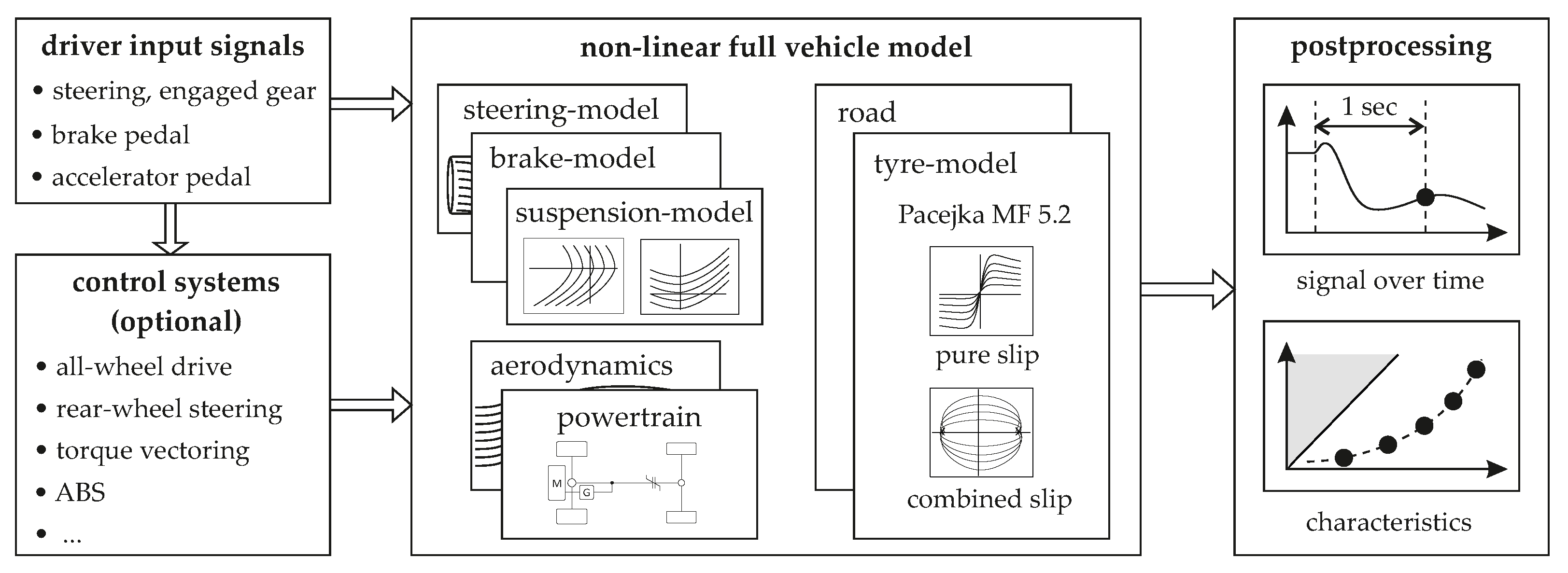
The derived AWD control is to be assessed by simulation based on MATLAB/SIMULINK
® (Release 2010b). A comprehensive non-linear full vehicle model with 14 degrees of freedom will be used for the assessment (see
Figure 8).
It consists of various validated sub-models (see [
27]) such as the steering model, brake-model, suspension model, tyre model and the powertrain model including the implemented torque-on-demand transfer case. Furthermore, a fully parameterised Magic Formula 5.2 according to
Pacejka [
28] is used as the tyre model. The suspension model is especially important for the correct calculation of the wheel loads. Therefore it contains the proper spring stiffness, damping rate, roll center height and the roll torque distribution of the vehicle. The elastokinematics are also implemented using maps that represent the movement of the wheel suspension under the action of forces. All characteristics and parameters are exported from a multi-body simulation model which in turn has been fully validated on the basis of real vehicle measurements.
Control systems can optionally be switched on in the simulation environment. They are controlled via simulated CAN bus communication. Apart from the all-wheel-drive control, no other chassis control systems are used for the investigation in this paper. In particular, the drive torque at the wheels is not restricted by traction control. In addition, the vehicle has open differentials on both axles, which symmetrically distribute the drive forces to the left and right tyre.
The derived AWD control is assessed by the driving maneuver “Power On Cornering“ (PON), see [
3,
29]. The maneuver sequence and the objectives of the investigation are described by
Rompe in [
29]. Out of a steady-state circular motion with a well-defined initial lateral acceleration
and a specified initial radius
, the vehicle is accelerated while maintaining the steering wheel angle. The amount of the imposed longitudinal acceleration
is determined by the accelerator pedal end position
. According to
Rompe the aim of the PON-maneuver is to examine the dynamic vehicle response to a sudden increase in driving forces. As a result of the imposed longitudinal acceleration
and thus the increase in longitudinal velocity, the vehicle will move away from the initial radius
. Both the amount and the distribution of the driving forces have a decisive influence on the vehicle response, as well as the sideforces given by the lateral acceleration (see [
29]).
The variation of the motion quantities yaw rate
and sideslip angle
are decisive criteria for evaluating the vehicle reaction. The time to compare the characteristic values is one second. The choice of a period of one second is justified with the average reaction time of the driver (see [
29]). The sideslip angle after one second is compared with the initial sideslip angle
of the steady-state cornering. In the case of the yaw rate deviation
, on the other hand, the yaw rate to be compared cannot be the steady-state yaw rate from initial circular motion, since the current driving speed no longer corresponds to the initial speed after one second. The reference yaw rate is the yaw rate of an imaginary reference vehicle, which moves at the current speed after one second
on the starting radius
:
In summary, the following parameters as shown in
Table 3 serve as evaluation criteria for the vehicle response. Due to industrial confidential agreements the scales are not reported in this work. Nevertheless, the normalised representation of graphs will provide all the information to entirely discuss quantitative statements.
Furthermore, for this paper, the driving maneuvers are carried out for two different road friction coefficients—on the one hand on a high friction level with
and, on the other hand, on a medium friction coefficient
. The latter should reflect the maximum friction coefficient between tyre and road surface in very wet conditions. Starting from a steady-state circular driving on a radius
and with a predetermined initial lateral acceleration of
= 6 m/s
2, the accelerator pedal is suddenly actuated up to a defined value. The maneuver is repeated twelve times for different accelerator pedal positions, which are listed in
Table 4.
6. Simulation Results
6.1. Simulation Results on Dry Conditions
In the following, the derived AWD control is first examined on dry pavement, i.e., on high friction level with
. The wetness coordination unit assumes “Wetness degree 0“ and the introduced application parameter
is set to one. The previously introduced characteristic
(
16) will be used for the distribution key—both for dry and, later, for wet road surfaces. The distribution key is finally determined as follows:
The results of the vehicle response with adaptive all-wheel-drive control on dry roads are compared with previously calculated results for a fixed drive torque distribution of
and
. For an overview, the three vehicle configurations to be examined are listed again in
Table 5.
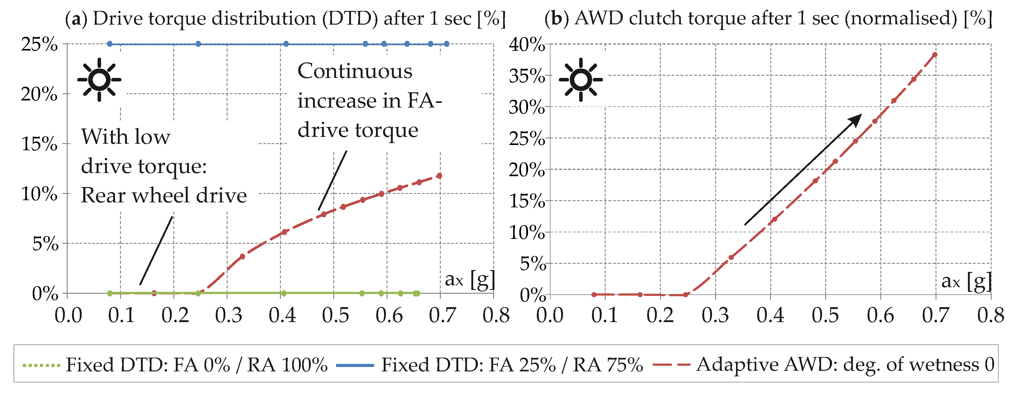
Figure 9a shows the course of the drive torque distribution (DTD) as a function of the achieved longitudinal acceleration
after 1s.
Up to an accelerator pedal position of
, the adaptive all-wheel-drive control does not put any drive torque to the front axle. This can be explained by the fact that the low required engine torque only leads to a low usage of the rear axle force potential. Ergo, the parameter
remains below
. Only from a longitudinal acceleration of
and with increasing accelerator pedal position
the AWD clutch torque increases as shown in
Figure 9b. At full throttle, the AWD achieves a maximum drive torque distribution of
.
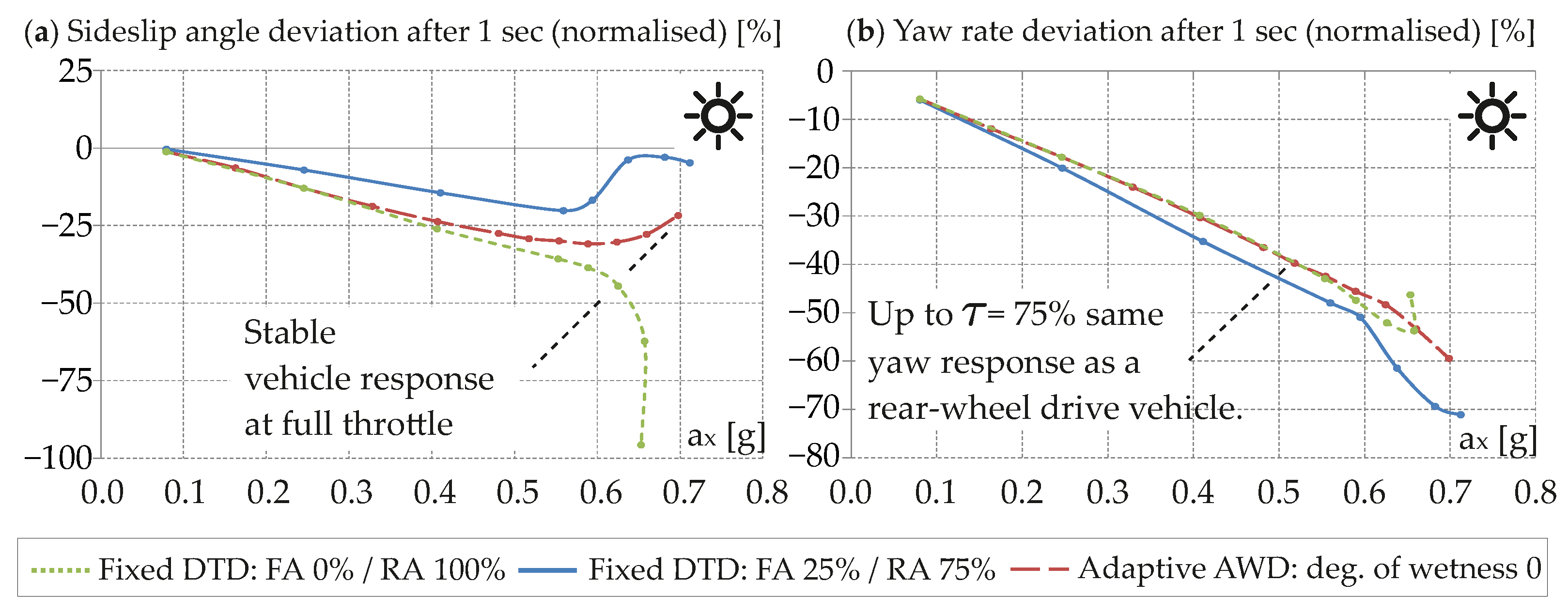
For the same simulation results,
Figure 10 shows (a) the sideslip angle deviation
and (b) the yaw rate deviation
after 1s in order to evaluate the vehicle response with regard to stability and agility. As before, in addition to the vehicle response with adaptive AWD control, the vehicle configurations with fixed drive torque distribution of
and
are also shown.
The vehicle with pure RWD becomes unstable when accelerating at full throttle (big negative sideslip angle). At low longitudinal acceleration, the vehicle with adaptive AWD and the vehicle with fixed rear-wheel-drive behave identically as long as the adaptive AWD control does not transmit any drive torque to the front axle. As the drive force on the front axle increases, the vehicle response with adaptive AWD diverges from that of the purely rear-wheel-drive vehicle in
Figure 10a. The slip angle deviation
is limited by the increasing DTD and the vehicle remains stable.
The initially purely rear-wheel drive torque distribution of the AWD vehicle leads to a very agile vehicle response—as can be seen in the yaw rate deviation
(see
Figure 10b). Even with medium AWD torque up to a throttle position of
, the yaw response of the AWD vehicle is almost identical to that of the purely RWD vehicle.
6.2. Simulation Results on Wet Conditions
In this section, three different controller settings are compared in order to examine the effectiveness of the wetness information implemented. The first setup is the adaptive all-wheel-drive with the assumption “degree of wetness 0“. The difference to driving maneuvers on dry roads (see
Section 6.1) is that the maximum friction coefficient is adjusted to the current value
. In the other two setups, the assumption for the degree of wetness is adjusted: “degree of wetness 1“ or “degree of wetness 2“. As a result, the introduced application parameter
is reduced to
or
according to
Figure 5. The same characteristic curve is selected as the distribution key
as in the tests on dry roads.
Table 6 shows the overview of the presented vehicle setups.
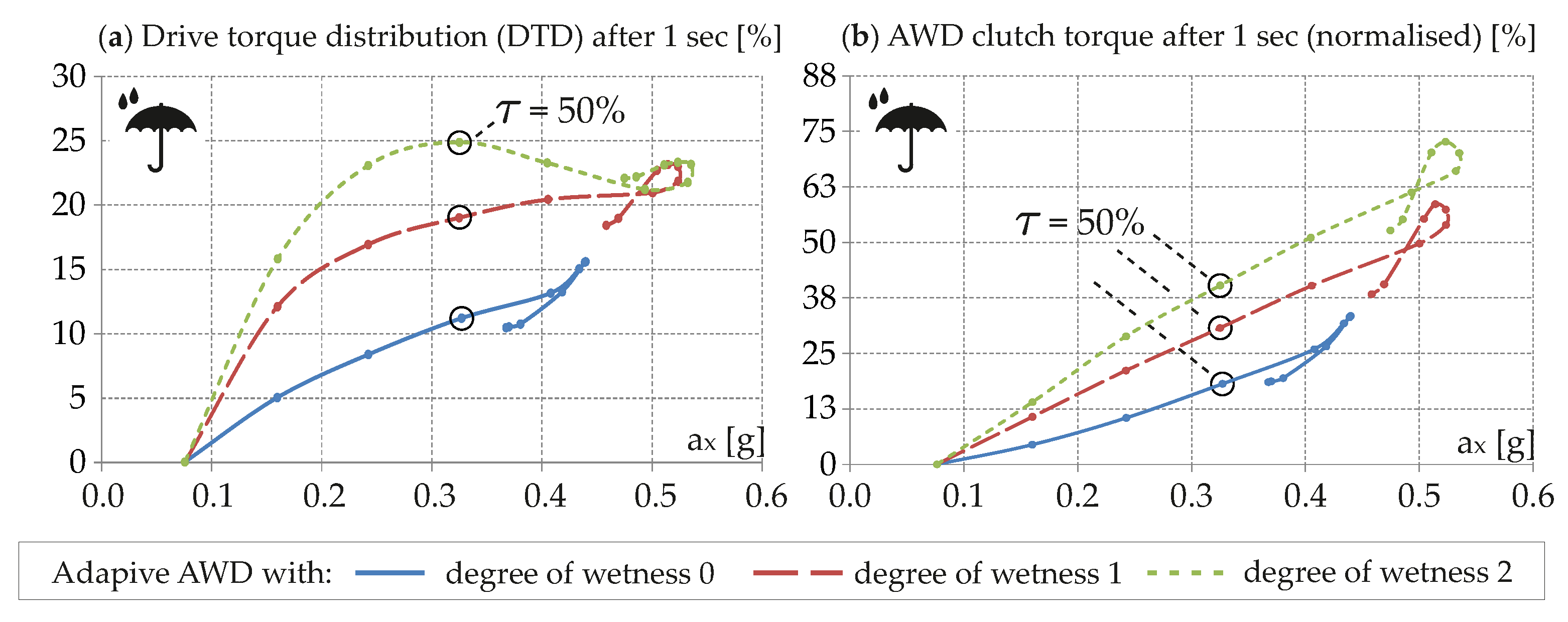
6.2.1. Drive Torque Distribution (DTD)
In
Figure 11, the DTD and the AWD clutch torque after one second are plotted as a function of the longitudinal acceleration
. While the drive force distribution achieves a maximum distribution of
with setup N0, a maximum DTD of
is achieved with setup N2. In all configurations, however, the maximum required AWD torque is below the component limit of the AWD clutch.
6.2.2. Stability and Agility
Figure 12 shows the slip angle deviation
and the yaw rate deviation
after one second as a function of the longitudinal acceleration
. The one-second characteristic values demonstrate that without specific intervention by the wetness coordination unit (vehicle with wetness degree zero) already from a longitudinal acceleration of
an unstable driving state occurs (see
Figure 12a).
When accelerating with an accelerator pedal actuation of , even the outer rear wheel reaches the adhesion limit and the vehicle response becomes unstable. When using the wetness coordination unit with degree of wetness two, the vehicle limit is only reached from an accelerator pedal actuation with . In addition, when the wetness coordination unit intervenes, a higher maximum longitudinal acceleration is achieved.
The favorable influence of the wetness coordination unit becomes even more clear when considering the maximum values for sideslip angle
and yaw rate
in
Figure 13.
Even at low longitudinal accelerations of approx. (corresponds to ) the controller setup “degree of wetness 2“ helps improve vehicle stability by dampening the overshoot behaviour of the vehicle response. In the highlighted example at , the front-biased DTD reduces the maximum sideslip angle deviation from to when setting the degree of wetness is two.
The higher damping of the vehicle yaw response through the use of the wetness coordination unit is also evident in the curve of the maximum yaw rate deviation. Due to the more front-biased DTD, the maximum yaw rate is significantly reduced from accelerations with a throttle position of . In the example presented at , the maximum yaw rate deviation is reduced from to .
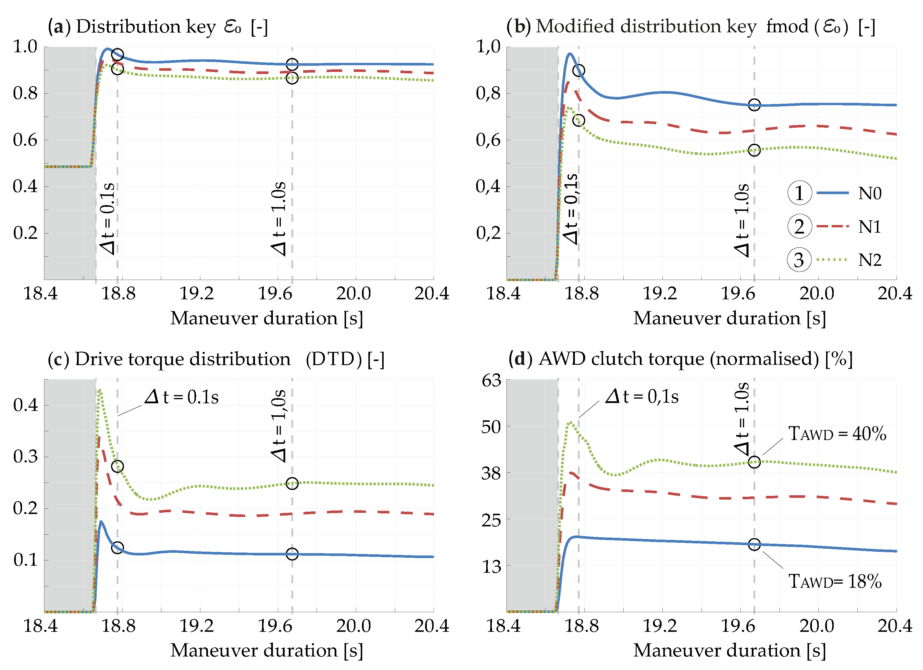
6.2.3. Insight into the Transient Vehicle Response
In addition to the analysis based on characteristic values after one second, the following section provides additional insight into the transient course of internal control variables and the vehicle motion. The period from the beginning of the maneuver to one second is considered and the result with a throttle position of
is analysed as an example.
Figure 14 shows internal controller variables in the time domain for a throttle end position of
. Togehter with the the motion quantities in
Figure 15 this provides more detailed insight into the course of the vehicle motion and into the influence of the AWD control. Before the start of the pedal actuation, the vehicle is in a steady-state circular motion. This period is highlighted in gray and is referred to as pre-maneuver.
During the steady-state pre-maneuver, the controller does not require any AWD torque on the front axle. The value of the calculated distribution key is
, see
Figure 14a. According to the self-map function from Equation (
19), however, a drive torque is only transmitted to the front axle from a value of
. The drive torque distribution and the AWD torque are, therefore, zero during the pre-maneuver, see
Figure 14c,d.
The period after the throttle is actuated clearly shows the differences between the three controller setups N0, N1 and N2. The increase in the traction forces of the rear axle leads to a non-vanishing function value for
since
exceeds the value of
, see
Figure 14a,b. After one second, the torque at the AWD clutch are twice as high for the setup“degree of wetness N2“ (
) as for the setup “degree of wetness N0“ (
), see
Figure 14d. This is due to the fact that with setup “N2“ more friction potential of the front axle is made available for traction in the calculation. The time courses also show an advantage of integrating the additional information “degree of wetness“ in a feedforward control. It can be seen that the feedforward AWD control makes the calculation of the internal control variables very fast and the AWD torque is requested very early. To emphasize this, the early point in time
s is highlighted as a reference.
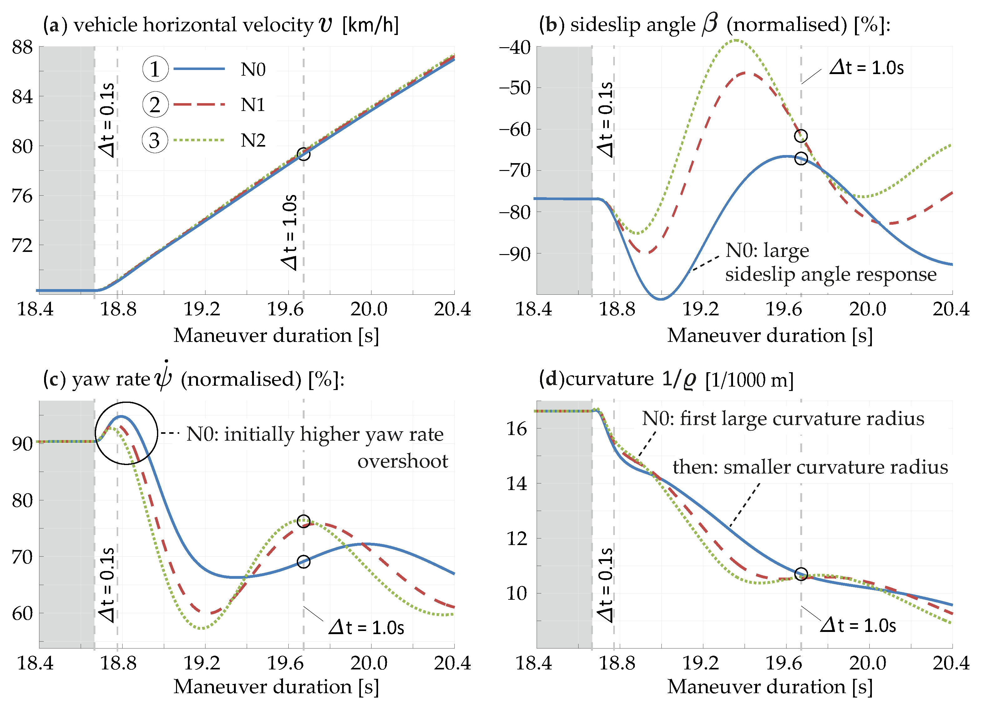
The different AWD torques for the three setups, N0, N1, N2, consequently lead to different vehicle responses. First of all, it is noticeable that the course of the vehicle speed is almost identical in all three variants. This means that the acceleration achieved is identical regardless of the AWD torque distribution. This is understandable because the traction limit is not yet reached with the throttle end position of . In contrast to this, the AWD distribution has a significant influence on the driving stability during the maneuver. This is shown by the vehicle motion quantities sideslip angle , yaw rate and curvature .
Basically, the vehicle response is stable for all three setups. Yet, the vehicle with controller setup “degree of wetness N0“ has the lowest vehicle stability. This is no longer shown only on the basis of the one-second value but is now even more noticeable, especially in the entire course of the sideslip angle, see
Figure 15b. With controller setup N0 a large negative sideslip angle
occurs on average and in absolute terms. The large sideslip angle results from the rear-biased drive torque distribution. For the present low friction coefficient, the driving forces on the rear axle are so high that the rear axle loses its lateral support. At the same time when looking at the yaw response, this leads to an initial yaw rate overshoot after the accelerator pedal has been actuated,
Figure 15c. Simultaneously, the vehicle briefly pushes towards the outside of the curve (see the large curvature radius in
Figure 15d accompanied by the increasing negative sideslip angle.
After the initial vehicle reaction, there is a change in the trajectory path in the early phase with setup N0. The sudden drop in the rear axle lateral forces first results in a large cornering radius of the trajectory path. Yet, as the vehicle’s longitudinal axis turns into the inside of the curve, the vehicle trajectory finally follows a small cornering radius in the further course, see
Figure 15d. In summary, it can be stated that, especially in critical drivinig situations under wet conditions, the aim is not to get such an unpredictable change in the path trajectory accompanied by a critical large sideslip angle response.
The opposite behaviour can be seen with controller setup N1 and N2. The front-biased drive torque distribution noticeably reduces the sideslip angle response and the vehicles do not reach a large negative sideslip angle
. Moreover, the initial yaw rate overshoot is reduced at the same time (see
Figure 15c).
7. Summary
A fundamental goal in the development of mechatronic chassis control systems is to generate a high level of functionality with a manageable number of understandable calibration parameters. The presented study makes a contribution to this in relation to an all-wheel-drive (AWD) system, which implements the information about road wetness that has recently become widely available. Moreover, the investigation shows the need to process information about existing road wetness in an all-wheel-drive system, despite knowledge of the friction coefficient.
In this research, a new concept for using road wetness information in an all-whell-drive (AWD) control has been presented. First, the AWD topology of a drive train with torque on demand transfer case was analysed. Under the assumption of quasi-stationary driving conditions, kinematic equations for the rotational speeds and torques were derived in this section. They served as the basis for calculating the wheel forces and torques in the AWD control that was later developed. After that, driving dynamics goals for the AWD under wet conditions were formulated. A particular focus was on the primary goals of stability and traction. Agility and power loss were cited as secondary goals, which must also be taken into account.
The starting point for the adaptive control strategy of the AWD was a state-of-the-art AWD control, which has been described in more detail. According to this basic AWD concept, parameters such as used friction potentials and remaining friction potentials are determined for each individual wheel from the precalculated wheel forces and from the currently assumed global friction potential . Subsequently, starting with the state-of-the-art AWD control as the basis, an adaptive control strategy is derived by superimposing a wetness coordination unit. This unit coordinates the optimal torque distribution through various interventions in the AWD control, which not only take into account the global friction coefficient , but also offer further options for intervention. The intervention takes place by using the following new parameters:
: modification of the remaining friction potential on the front axle ;
: shaping of a self-map function, called modified distribution key; and
: calculation of a friction deficit on the rear axle in the event of excess torque.
The derived AWD control has been assessed by simulation in a non-linear full vehicle model with 14 degrees of freedom and by using the driving maneuver “Power On Cornering“ (PON), which means an acceleration out of steady-state circular motion.
8. Conclusions and Outlook
As the essential benefit, the developed all-wheel-drive (AWD) control enables a maximum spread between driving stability, agility and traction under combined vehicle dynamics when using wetness information. With the newly introduced wetness coordination unit, the derived AWD control no longer just takes into account the current friction coefficient. The adhesion limit is important in order to calculate the current usage of the longitudinal force potential of the tyres. However, this only ensures that the maximum traction potential of the tyres is not exceeded. The wetness coordination unit now enables the driving dynamics targets to be adjusted using the wetness information within the frictional adhesion limits. All of this is done through AWD control using only a few additional and physically interpretable key parameters and without significantly increasing the controller complexity.
As a result, on dry roads the derived control concept shows a rear-biased drive torque distribution (DTD) at low and medium requested drive torques. At low accelerations below 0.25 g, the vehicle even operates as a pure rear-wheel-drive (RWD) vehicle. This decreases the mechanical component stress of the clutch and it reduces the occurring power loss. Only when the accelerator pedal is raised, the DTD increases to such an extent that the vehicle does not become unstable under full throttle.
On wet roads the limit of vehicle stability can be shifted towards higher longitudinal accelerations by the adaption of the new calibration parameters. At the same time, traction is improved and the vehicle achieves higher longitudinal acceleration values. The vehicle stability limit was only reached when the accelerator pedal actuation is more or equal to . Another advantageous point is the yaw dampening effect of the increased AWD torque. When considering the amount of drive torque distribution, it also shows that if the friction potential is used to a small extent (low longitudinal accelerations), only a low AWD torque is required. This was one of the basic properties of the basic AWD control, which was retained after the expansion of the AWD torque control for wet conditions. With low drive forces, this relieves the mechanical component stress of the clutch—even in wet conditions.
In summary, it can be stated that the extended approach fulfills the primary requirements made previously. As already supposed, it was not enough to adjust the assumed global friction potential in the controller; the driving dynamics targets in wet conditions must also be adjusted. The approach also fulfills the secondary requirements, especially when the vehicle is still far enough away from the vehicle stability limit.
For subsequent investigations, further control systems with great influence on driving stability in the vehicle dynamic limits should be included in the concept. As a first suggestion the AWD control should be especially extended and examined for torque vectoring systems, which enable a lateral torque distribution in addition. Then as a next step, the influence of an active roll torque distribution system can be taken into account. As soon as the number of control systems increases, the classic control scheme as presented here must then also be compared with approaches from central control and with approaches from optimal control, which are especially advantageous for quadratic multiple-input–multiple-output systems [
30] or even for overactuated systems [
31,
32].
Author Contributions
Conceptualization, G.W.; methodology, G.W.; software, G.W.; validation, G.W., investigation, G.W.; writing–original draft preparation, G.W.; writing—review and editing, P.S., M.U. and D.S.; supervision, P.S., M.U. and D.S.; project administration, D.S.; funding acquisition, D.S. All authors have read and agreed to the published version of the manuscript.
Funding
This research received no external funding.
Institutional Review Board Statement
Not applicable.
Informed Consent Statement
Not applicable.
Data Availability Statement
Not applicable.
Acknowledgments
We acknowledge support by the Open Access Publication Fund of the University of Duisburg-Essen.
Conflicts of Interest
The authors declare no conflict of interest.
Abbreviations
| ABS | anti-lock braking system |
| ADAS | advanced driver assistance systems |
| AFS | active front steering system |
| AWD | all-wheel-drive |
| DTD | drive torque distribution |
| ESP | electronic stability program |
| FA | front axle |
| FL | front left |
| FR | front right |
| GO | gearbox output |
| PON | power-on-cornering maneuver |
| RA | rear axle |
| RL | rear left |
| RR | rear right |
| adapt | adaptive |
| eng | engine |
| est | estimated |
| i | placeholder for F (front axle), R (rear axle) |
| j | placeholder for L (left tyre), R (right tyre) |
| max | maximum |
| mod | modified |
| over | overshoot, excess |
| pot | potential |
| ref | reference |
Appendix A. Nomenclature
Table A1.
List of symbols and abbreviations.
Table A1.
List of symbols and abbreviations.
| Dimensionless Properties | | Description |
| [-] | global friction coefficient |
| [-] | used friction potential |
| [-] | remaining friction potential for traction |
| [-] | friction deficit on the rear axle |
| [-] | traction potential transferred in the event of excess |
| [-] | parameter for degression of friction coefficient |
| [-] | distribution key for the AWD torque |
| [-] | first calibration parameter (self-map) |
| [-] | second calibration parameter |
| , | [-] | front, rear axle differential ratio |
| [-] | steering ratio |
| [%] | accelerator pedal actuation |
| Distances | Unit | Description |
| [m] | center of gravity height |
| [m] | front, rear semi-wheelbase |
| , | [m] | front, rear axle dynamic rolling radius |
| [m] | curvature radius of the vehicle trajectory |
| [m] | initial radius (steady-state cornering) |
| Torques | Unit | Description |
| , | [Nm] | front, rear axle drive torque |
| [Nm] | main driveshaft torque |
| [Nm] | gearbox output torque |
| [Nm] | engine-sided driveshaft torque |
| [Nm] | AWD torque (clutch) |
| Forces | Unit | Description |
| , , | [N] | longitudinal, lateral, vertical tyre force |
| , | [N] | front, rear axle traction force (sum of both tyres) |
| , | [N] | front, rear axle potential traction force |
| [N] | drive force excess |
| [N] | nominal wheel load |
| Angles and Angular Velocities | Unit | Description |
| [rad] | steering wheel angle |
| [rad] | sideslip angle |
| [rad/s] | yaw velocity |
| , | [rad/s] | front, rear axle rotational speed |
| , | [rad/s] | front, rear axle rotational speed |
| [rad/s] | gearbox output rotational speed |
| [rad/s] | engine speed |
| Miscellaneous properties | Unit | Description |
| g | [] | gravitational field strength |
| , | [] | longitudinal, lateral acceleration |
| m | [kg] | vehicle mass |
| [W] | power loss (torque-on-demand transfer case) |
References
- Zomotor, A. Fahrwerktechnik: Fahrverhalten; Vogel Fachbuch: Wuerzburg, Germany, 1991; p. 178. ISBN 3802307747. [Google Scholar]
- Preukschat, A. Fahrwerktechnik: Antriebsarten; Vogel Fachbuch: Wuerzburg, Germany, 1988; p. 136. ISBN 3802307364. [Google Scholar]
- Heißing, B.; Ersoy, M. Chassis Handbook—Fundamentals, Driving Dynamics, Components, Mechatronics, Perspectives, 1st ed.; Springer Fachmedien: Wiesbaden, Germany, 2011; pp. 145–162. ISBN 9783834809940. [Google Scholar]
- Fuchß, S.; Wieland, D.; Siebert, N.; Hitzfeld, H.; Weber, H.-P.; Trost, M.; Gaupp, A.; Schröder, R.; Leucht, M. All-Wheel Drive for Stability, Comfort, and Handling. Atzextra Worldw. 2009, 14, 144–148. [Google Scholar] [CrossRef]
- Meißner, T.C. Verbesserung der Fahrzeugquerdynamik Durch Variable Antriebsmomentenverteilung. Ph.D. Thesis, Institut für Maschinen und Fahrzeugtechnik—Lehrstuhl für Fahrzeugtechnik, TU München, Munchen, Germany, 2008; p. 107. [Google Scholar]
- Weber, I. Verbesserungspotenzial von Stabilisierungssystemen im Pkw durch eine Reibwertsensorik. Ph.D. Thesis, Fachbereich Maschinenbau, Technischen Universität, Darmstadt, Germany, 2004. [Google Scholar]
- Singh, K.B.; Sivaramakrishnan, S. An Adaptive Tire Model for Enhanced Vehicle Control Systems. SAE Int. J. Passeng. Cars Mech. Syst. 2015, 8, 128–145. [Google Scholar] [CrossRef]
- Genegenbach, W. Das Verhalten von Kraftfahrzeugreifen auf trockener und insbesondere nasser Fahrbahn. Ph.D. Thesis, Institut für Maschinenkonstruktionslehre und Kraftfahrzeugbau, Universität Karlsruhe (TH), Karlsruhe, Germany, 1967. [Google Scholar]
- Parment, A. Die Zukunft des Autohandels, 1st ed.; Springer Fachmedien: Wiesbaden, Germany, 2016; pp. 54–61. ISBN 9783658078867. [Google Scholar]
- Gnadler, R.; Unrau, H.-J. Method and Device for Determining the Adhesion and Adhesion Limit for Vehicle Tyres. Pub. No. WO 00/32456, 1 December 1998. [Google Scholar]
- Stellet, J.; Suchanek, A.; Gießler, M.; Puente León, F.; Gauterin, F. Fahrbahnreibwertschätzung mit optimaler linearer Parametrierung. Automatisierungstechnik 2014, 62, 570–781. [Google Scholar] [CrossRef]
- Lex, C. Estimation of the Maximum Coefficient of Friction between Tire and Road Based on Vehicle State Measurements. Ph.D. Thesis, Institute of Automotive Engineering, Graz, Austria, 2015. [Google Scholar]
- Roychowdhury, S.; Zhao, M.; Wallin, A.; Ohlsson, N.; Jonasson, M. Machine Learning Models for Road Surface and Friction Estimation using Front-Camera Images. In Proceedings of the International Joint Conference on Neural Networks (IJCNN), Rio de Janeiro, Brazil, 8–13 July 2018; pp. 1–8. [Google Scholar]
- Song, S.; Min, K.; Park, J.; Kim, H.; Huh, K. Estimating the Maximum Road Friction Coefficient with Uncertainty Using Deep Learning. In Proceedings of the 21st International Conference on Intelligent Transportation Systems (ITSC), Maui, HI, USA, 4–7 November 2018; pp. 3156–3161. [Google Scholar]
- Hartmann, B.; Eckert, A. Road Condition Observer as a New Part of Active Driving Safety. Atzelectronics Worldw. 2017, 12, 34–37. [Google Scholar] [CrossRef]
- Görich, H.-J.; Jacobi, S. Detecting Moisture on Road Surface from Vehicle. Pub. No. DE 42 13 221 A1, 11 April 1992. [Google Scholar]
- Müller, G.; Müller, S. Method for Estimating of the Friction Potential. ATZ Worldw. 2016, 6, 58–63. [Google Scholar] [CrossRef]
- Alonso, J.; López, J.M.; Pavón, I.; Recuero, M.; Asensio, C.; Arcas, G.; Bravo, A. On-board wet road surface identification using tyre/road noise and Support Vector Machines. Appl. Acoust. 2014, 76, 407–415. [Google Scholar] [CrossRef]
- Abdić, I.; Fridman, L.; Brown, D.E.; Angell, W.; Reimer, B.; Marchi, E.; Schuller, B. Detecting Road Surface Wetness from Audio: A Deep Learning Approach. In Proceedings of the 23rd International Conference on Pattern Recognition (ICPR), Cancún, Mexico, 4–8 December 2016; pp. 3458–3463. [Google Scholar]
- Billet, Y. Detection of wet road conditions in the new generation of the 911. In Proceedings of the 10th International Munich Chassis Symposium 2019; Pfeffer, P.E., Ed.; Springer Fachmedien Wiesbaden: Wiesbaden, Germany, 2020; pp. 71–83. ISBN 9783658264352. [Google Scholar]
- High Driving Stability Even in the Rain. Available online: https://newsroom.porsche.com/en/products/porsche-911-new-eigth-generation-992-timeless-machine-design-icon-wet-mode-detecting-wet-road-conditions-16857.html (accessed on 19 December 2021).
- Schmiedel, B.; Gauterin, F.; Unrau, H.-J. Road wetness quantification via tyre spray. Proc. Inst. Mech. Eng. Part D J. Automob. Eng. 2019, 233, 28–37. [Google Scholar] [CrossRef]
- Bartels, H.; Pascali, L.; Mack, G.; Huneke, M. Method for Distributing a Requested Torque. Pub. No. US 2014/0172215 A1, 19 June 2014. [Google Scholar]
- Schramm, D.; Hiller, M.; Bardini, R. Vehicle Dynamics—Modeling and Simulation, 1st ed.; Springer: Berlin/Heidelberg, Germany, 2014; p. 198. ISBN 9783540360452. [Google Scholar]
- Bartels, H.; Pascali, L.; Mack, G.; Huneke, M. Verfahren zum Verteilen eines Wunschdrehmomentes. Offenlegungsschrift beim. Deutschen Patent und Markenamt Pub. No. DE 10 2012 112 418 A1, 18 June 2014. [Google Scholar]
- Mitschke, M.; Wallentowitz, H. Dynamik der Kraftfahrzeuge, 4th ed.; Springer VDI: Berlin/Heidelberg, Germany, 2004; pp. 723–726, 733. ISBN 3540420118. [Google Scholar]
- Peters, Y.; Stadelmayer, M. Control allocation for all wheel drive sports cars with rear wheel steering. Automot. Engine Technol. 2019, 4, 119. [Google Scholar] [CrossRef]
- Pacejka, H.B. Tyre and Vehicle Dynamics, 2nd ed.; Elsevier-Verlag: Oxford, UK, 2006; ISBN 9800750669184. [Google Scholar]
- Rompe, K.; Heißing, B. Fahrzeugtechnische Schriftenreihe—Objektive Testverfahren für die Fahreigenschaften von Kraftfahrzeugen, 1st ed.; Verlag TÜV Rheinland GmbH: Koln, Germany, 1984; pp. 67–69. ISBN 3885851318. [Google Scholar]
- Warth, G.; Frey, M.; Gauterin, F. Design of a central feedforward control of torque vectoring and rear-wheel steering to beneficially use tyre information. Veh. Syst. Dyn. 2020, 58, 1789–1822. [Google Scholar] [CrossRef]
- Schwartz, M.; Siebenrock, F.; Hohmann, S. Model predictive control allocation of an over-actuated electric vehicle with single wheel actuators. In Proceedings of the 10th IFAC Symposium on Intelligent Autonomous Vehicles IAV 2019, Gdansk, Poland, 3–5 July 2019; Volume 52, pp. 162–169. [Google Scholar] [CrossRef]
- Sieberg, P.; Schramm, D. Central Non-linear Model-Based Predictive Vehicle Dynamics Control. Appl. Sci. 2021, 11, 4687. [Google Scholar] [CrossRef]
Figure 1.
Driving mode selection in the Porsche 959 (1986–1988). Operated manually by the driver. [Source: Porsche AG].
Figure 1.
Driving mode selection in the Porsche 959 (1986–1988). Operated manually by the driver. [Source: Porsche AG].
Figure 2.
(a) Torque and (b) rotational speed in the powertrain of an all-wheel-drive vehicle with torque-on-demand transfer case.
Figure 2.
(a) Torque and (b) rotational speed in the powertrain of an all-wheel-drive vehicle with torque-on-demand transfer case.
Figure 3.
Used friction potential at PON-maneuver: (a) Schematic representation on the quasi-static twin-track model. (b) Used friction potential and remaining friction potential on the outside wheel of the front axle and (c) on the outside wheel of the rear axle.
Figure 3.
Used friction potential at PON-maneuver: (a) Schematic representation on the quasi-static twin-track model. (b) Used friction potential and remaining friction potential on the outside wheel of the front axle and (c) on the outside wheel of the rear axle.
Figure 4.
Overview of the overall concept of the extended all-wheel-drive control with superordinate wetness coordination unit. Newly created parameters allow a specific calibration for wetness.
Figure 4.
Overview of the overall concept of the extended all-wheel-drive control with superordinate wetness coordination unit. Newly created parameters allow a specific calibration for wetness.
Figure 5.
Concept idea—variable consideration of the required lateral friction potential of the front axle tyres depending on the assumed degree of wetness.
Figure 5.
Concept idea—variable consideration of the required lateral friction potential of the front axle tyres depending on the assumed degree of wetness.
Figure 6.
Concept idea—calculation of an excess torque and of a friction deficit on the rear axle when approaching full throttle.
Figure 6.
Concept idea—calculation of an excess torque and of a friction deficit on the rear axle when approaching full throttle.
Figure 7.
Self-map function: function course of a modified distribution key .
Figure 7.
Self-map function: function course of a modified distribution key .
Figure 8.
Sheme of the simulation environment with subsequent postprocessing.
Figure 8.
Sheme of the simulation environment with subsequent postprocessing.
Figure 9.
“Power On Cornering“ maneuver ( = 6 m/s2) on dry road (): (a) drive torque distribution (DTD) after 1s; (b) normalised AWD clutch torque after 1s.
Figure 9.
“Power On Cornering“ maneuver ( = 6 m/s2) on dry road (): (a) drive torque distribution (DTD) after 1s; (b) normalised AWD clutch torque after 1s.
Figure 10.
“Power On Cornering“ maneuver () on dry road (): (a) sideslip angle difference after 1s; (b) yaw rate difference after 1s.
Figure 10.
“Power On Cornering“ maneuver () on dry road (): (a) sideslip angle difference after 1s; (b) yaw rate difference after 1s.
Figure 11.
“Power On Cornering“ maneuver () on wet road (): (a) drive torque distribution (DTD) after 1s; (b) normalised AWD clutch torque after 1s.
Figure 11.
“Power On Cornering“ maneuver () on wet road (): (a) drive torque distribution (DTD) after 1s; (b) normalised AWD clutch torque after 1s.
Figure 12.
“Power On Cornering“ maneuver () on wet road (): (a) sideslip angle difference after 1s; (b) Yaw rate difference after 1s.
Figure 12.
“Power On Cornering“ maneuver () on wet road (): (a) sideslip angle difference after 1s; (b) Yaw rate difference after 1s.
Figure 13.
“Power On Cornering“ maneuver () on wet road (): (a) maximum to steady-state sideslip angle; (b) maximum to steady-state yaw rate.
Figure 13.
“Power On Cornering“ maneuver () on wet road (): (a) maximum to steady-state sideslip angle; (b) maximum to steady-state yaw rate.
Figure 14.
Internal controller parameters during “Power On Cornering“ maneuver () on wet road (): (a) distribution key ; (b) modified distribution key ; (c) drive torque distribution; (d) AWD clutch torque.
Figure 14.
Internal controller parameters during “Power On Cornering“ maneuver () on wet road (): (a) distribution key ; (b) modified distribution key ; (c) drive torque distribution; (d) AWD clutch torque.
Figure 15.
Vehicle motion during “Power On Cornering“ maneuver () on wet road (): (a) vehicle velocity; (b) sideslip angle; (c) yaw rate; (d) curvature of the trajectory.
Figure 15.
Vehicle motion during “Power On Cornering“ maneuver () on wet road (): (a) vehicle velocity; (b) sideslip angle; (c) yaw rate; (d) curvature of the trajectory.
Table 1.
Overview and calculation of the rotational speeds and torques in an all-wheel-drive vehicle with torque-on-demand transfer case.
Table 1.
Overview and calculation of the rotational speeds and torques in an all-wheel-drive vehicle with torque-on-demand transfer case.
| Subsystem | Symbol | Equation |
|---|
| Rotational speeds: | | |
| gearbox output | | |
| main drive shaft | | |
| rear axle differential | | |
| front axle differential | | |
| Torques: | | |
| gearbox output | | |
| main drive shaft | | |
| rear axle differential | | |
| front axle differential | | |
| Power loss: | | |
| AWD clutch | | |
Table 2.
Basic equations from the patent application [
23,
25] “Method for distributing a requested torque“ including the extensions for the study.
Table 2.
Basic equations from the patent application [
23,
25] “Method for distributing a requested torque“ including the extensions for the study.
| Calculation Module | Equation |
|---|
| Friction coefficient: | |
| Friction coefficient (load dependend) | |
| Tyre forces: | |
| wheel loads | |
| axle sideforces | |
| wheel sideforces | |
| Used friction potential: | |
| used friction potential (longitudinal) | |
| used friction potential (lateral) | |
| used friction potential (global) | |
| Remaining friction potential: | |
| remaining friction potential (longitud.) FA | |
| remaining friction potential (longitud.) RA | |
Table 3.
Assessment criteria for the PON driving-maneuver.
Table 3.
Assessment criteria for the PON driving-maneuver.
| Characteristics | Unit | Description |
|---|
| [rad/s] | yaw rate deviation after 1s |
| [deg] | sideslip angle deviation after 1s |
| [deg] | maximum sideslip angle deviation |
| [-] | max. yaw rate deviation (as ratio to reference yaw rate) |
| [%] | Drive Torque Distribution after 1s |
| [Nm] | AWD clutch torque after 1s |
Table 4.
Accelerator pedal end position for the PON-maneuver.
Table 4.
Accelerator pedal end position for the PON-maneuver.
| | | | | | | | | | | |
|---|
| | | | | | | | | | | |
Table 5.
Overview of the vehicle configurations and constraints for the investigation of the driving dynamics on dry pavement.
Table 5.
Overview of the vehicle configurations and constraints for the investigation of the driving dynamics on dry pavement.
| Naming | Maneuver Params | Controller Parameters | | | | | |
|---|
| Setup | | | AWD | | | | |
|---|
| fixed DTD | 60 m | | | - | - | - | - |
| fixed DTD | 60 m | | | - | - | - | - |
| Adapt. N0 | 60 m | | adaptive | | 0 | | 70% |
Table 6.
Overview of the vehicle configurations and constraints for the investigation of the driving dynamics on wet pavement.
Table 6.
Overview of the vehicle configurations and constraints for the investigation of the driving dynamics on wet pavement.
| Naming | Maneuver Params. | Controller Parameters |
|---|
| Setup | | | AWD | | | | |
|---|
| Adapt. N0 | | | adaptive | | 1 | | 70% |
| Adapt. N1 | | | adaptive | | | | 70% |
| Adapt. N2 | | | adaptive | | 0 | | 70% |
| Publisher’s Note: MDPI stays neutral with regard to jurisdictional claims in published maps and institutional affiliations. |
© 2022 by the authors. Licensee MDPI, Basel, Switzerland. This article is an open access article distributed under the terms and conditions of the Creative Commons Attribution (CC BY) license (https://creativecommons.org/licenses/by/4.0/).


