Abstract
Different risks are associated with the operation and maintenance of wind farms in cold climate regions, mainly due to the harsh weather conditions that wind farms experience in that region such as the (i) increased stoppage rate of wind turbines due to harsh weather conditions, (ii) limited accessibility to wind farms due to snow cover on roads, and (iii) cold stress to workers at wind farms. In addition, there are risks that are caused by wind farms during their operation, which impact the surrounding environment and community such as the (iv) risk of ice throw from wind turbines, (v) environmental risks caused by the wind farms, and (vi) social opposition risk to installing wind farms in cold climate regions, such as the Arctic. The analysis of these six risks provides an overall view of the potential risks encountered by designers, operators, and decision makers at wind farms. This paper presents a methodology to quantify the aforementioned risks using fuzzy logic method. At first, two criteria were established for the probability and the consequences of each risk; with the use of experts’ judgments, membership functions were graphed to reflect the two established criteria, which represented the input to the risk analysis process. Furthermore, membership functions were created for the risk levels, which represented the output. To test the proposed methodology, a wind farm in Arctic Norway was selected as a case study to quantify its risks. Experts provided their assessments of the probability and consequences of each risk on a scale from 0–10, depending on the description of the wind farm provided to them. Risk levels were calculated using MATLAB fuzzy logic toolbox and ranked accordingly. Limited accessibility to the wind farm was ranked as the highest risk, while the social opposition to the wind farm was ranked as the lowest. In addition, to demonstrate the effects of the Arctic operating conditions on performance and safety of the wind farm, the same methodology was applied to a wind farm located in a non-cold-climate region, which showed that the risks ranked differently.
1. Introduction
Wind energy applications in cold climate regions (CCRs) have gained more attention recently, and are growing at a rapid rate of approximately 20% per year according to the Global Wind Energy Council [1]. There are various encouraging reasons for installing wind farms (WFs) in CCRs: among others, the fact that the density of air in such regions is 10% higher than other non-cold climate regions, which results in higher availability of wind power resources [2]. In addition, abundant air resources exist in mountainous CCRs such as the Arctic region of Norway, where relatively steady winds with higher velocities [3]. Moreover, CCRs are known to be less and sparsely inhabited than other regions in the same country. Therefore, having WFs installed there will have less perceived impact on people than WFs built in large cities for example, and will likely encounter less opposition to installing WFs from residents.
CCRs are characterized by an air temperature of less than −20 °C, lasting for at least nine days per year, and an average annual temperature of less than 0 °C [4]. Wind turbines (WTs) in CCRs experience temperatures below their standard operational limits and may experience incidents of icing conditions. Therefore, such weather conditions can result in risks that will have negative impacts on WFs, and can consequently affect their surrounding environment and community.
The discussed risks in this paper are described to be emerging either from the harsh weather conditions in CCRs that affect the operation and maintenance of WFs, or risks that emerge from the WFs that affect their surrounding environment and community. The first type of risks that emerge from harsh weather conditions include the very cold temperatures and the ice accretion on the blades of WTs, which will increase the failure rate of the blades and other WT components [5,6], leading to increased operation stoppage rate of WTs. In addition, very cold temperatures can cause cold stress to workers at WFs, and might result in injuries, leading to reduced dexterity of workers and delaying maintenance of defected WTs [7]. Moreover, excessive snow precipitation can limit the accessibility to WFs, which can affect the maintenance activities required to maintain a certain level of performance. Therefore, snow removal strategies and specially equipped vehicles have to be used to overcome this risk [4]. On the other hand, the second type of risks that emerge from WFs include the ice throw from WTs caused by the centrifugal force of the WTs and the melting of ice on the blades, which can be harmful to workers at the WF, nearby residents, and other infrastructures and animals [8]. Furthermore, there are the environmental risks, which can be critical especially in the Arctic region, which is famous for its sensitive environment (with vulnerable bird and mammal species); lastly, there is the social opposition from the surrounding community that can negatively affect the wind energy investments in CCRs [9].
Careful analysis of the aforementioned risks is mandatory to control them and mitigate their probability of occurrence and the severity of their consequences. Moreover, analyzing these risks represents an input to the risk evaluation step in the risk management process and to the risk treatment step [10]. Additionally, this paper provides inputs to several wind energy research fields such as the optimization of the WT performance [7,11,12], in which the cold climate operating conditions are a major contributor to degrading the performance of WFs installed in that region, which likewise applies to WT power curves [13,14], WT blades [15,16], and WT life [17,18] research fields.
Furthermore, this paper aims at providing an overall analysis and ranking of these risks, which can help designers of WFs, risk managers, and operators acquire a holistic image of the potential risks, which will contribute to the prioritizing of their decisions in case of the lack of sufficient data that is usually encountered in CCRs, due to the fact that wind energy applications in that region are relatively new [4].
One of the effective tools for analyzing and ranking risks in the absence of quantitative probability models is fuzzy logic [19]. Fuzzy logic can make use of experts’ judgments and available data to model the inaccuracy and uncertainty in human thinking [20], which can create confusion when using vague linguistic terms such low, medium, high, etc. Risks are measured quantitatively using fuzzy logic, which increases the accuracy of ranking the risks and accurately prioritizes risk control measures. Fuzzy logic has been applied in different applications. For example, Fuzzy Failure Mode and Effects Analysis (Fuzzy FMEA) has been developed and applied by [19,21] to rank the failures in different WT components, and in determining the costs of failure to WTs [22]. Fuzzy logic was also used for risk assessment of pipelines transporting flammable substances [23], and offshore engineering systems [24].
This paper utilizes fuzzy logic and experts’ judgments to rank six types of risks to and from WFs in CCRs, mainly in the Arctic region. Furthermore, the paper compares the ranking of the same risks to a similar WF that is installed in a non-cold-climate region, to demonstrate the Arctic effects on the WF.
The paper is organized as follows: Section 2 presents the methodology followed to analyze the risks. Section 3 explains the fuzzy logic process. Section 4 identifies six risks to WFs in CCRs. Section 5 defines the criteria for the risks, considering five levels of probabilities (very low, low, medium, high, very high) and four for the severity of consequences (low moderate, high, very high). Section 6 considers a WF in Arctic Norway as a case study to demonstrate the proposed methodology and ranks the six risks; finally, conclusions are presented in Section 7.
2. Methodology
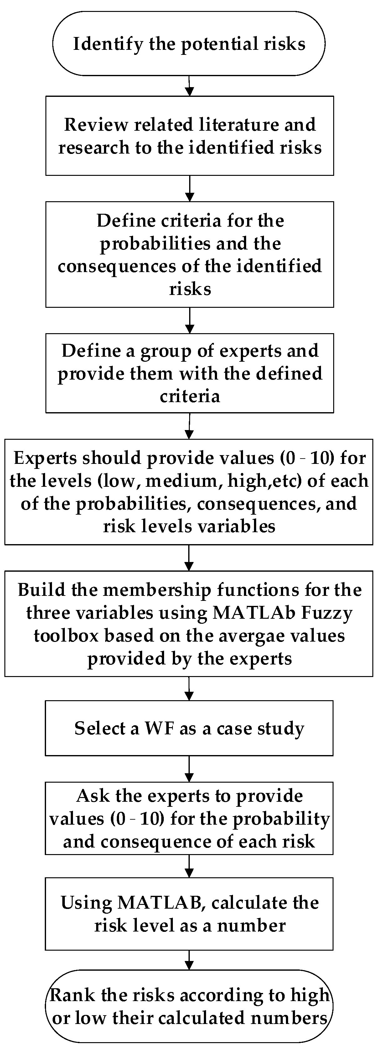
The methodology adopted in this work, shown in Figure 1, starts with identifying the potential risks usually WFs in CCRs are subjected to. The risks-relevant literature and research are being reviewed to define criteria for the inputs to the risk analysis, which are the probabilities of occurrence and the severity of consequences of the identified risks. Afterwards, the defined criteria are sent to a selected group of experts who will provide estimated values (between 0 and 10) for the different levels of the probabilities and consequences, which represent the input to the risk analysis and for the risks’ levels, which represents the output. Based on the data collected from the experts, and by using MATLAB fuzzy logic toolbox, membership functions are graphed to represent the levels of the inputs and the output.
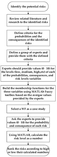
Figure 1.
Methodology of analyzing risks to WFs in CCRs using fuzzy logic.
This methodology is implemented to a WF in Arctic Norway as a case study for demonstration. Initially, data regarding the WF are gathered from the WF operator, research articles, and weather stations that publish their data online. Afterwards, the collected data conceded to a selected group of experts, who are asked to quantitatively evaluate the corresponding probability of occurrence and severity of consequences of each of the identified risks on a scale from 0 to 10. Experts’ judgments were then fed into MATLAB fuzzy logic toolbox, which calculated the risk level, using specifically defined rules. Eventually, the risks are ranked depending on the resulting risk level, the highest risk level was assigned a rank of (1) and the lowest risk was assigned a rank of (6).
3. Fuzzy Logic Process
Fuzzy logic is based on fuzzy set theory developed by Zadeh [25]. Fuzzy sets are a generalization of the classical set theory, indicating that the classical set theory is a special case of the fuzzy set theory [26]. Fuzzy logic is an efficient tool in risk assessment as it compensates for the lack of knowledge and vagueness encountered when assessing the risks related to complex technological systems, and can be very helpful when dealing with fuzzy linguistic terms such as low, medium, high, etc., to describe the risks, as these terms do not have sharp boundaries for their definitions and can hold different interpretations when interpreted by different experts [23].
For example, taking X as a universal set that contains all objects used in the risk analysis process. Probability, consequences, and risk levels are the input and output variables used in the risk analysis. Each one of these variables contains a number of objects (fuzzy terms) that were previously defined in X as follows:
- X = {very low, low, medium, moderate, high, very high, moderate-high, extremely high}
- Input variable (probability) = {very low, low, medium, high, very high}
- Input variable (consequences) = {low, moderate, high, very high}
- Output variable (risk level) = {very low, low, moderate, moderate-high, high, very high, and extremely high}
Each fuzzy term in the universal set X is described as a fuzzy subset (A), characterized by a membership function μ(x), which assigns to each object a degree of membership that has values between zero (no-membership) and one (complete membership). Based on that, a fuzzy subset A can be written as a set of pair: A = {(x,μA(x)); x∈X}, where x is a numbering value provided by the experts to describe the input variable (i.e., the probability or the consequences) [23].
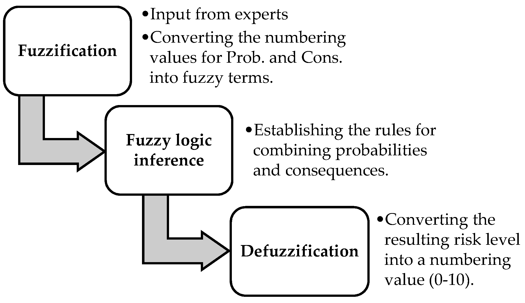
The fuzzy logic process followed in this paper is based on Mamdani method [27], which is the most commonly used method in fuzzy logic, using the center of gravity method to calculate the output value of the risk level during the defuzzification step, unlike the Sugeno method, which uses the weighted average method to calculate the risk level [28]. Figure 2 shows the three main steps (fuzzification, fuzzy logic inference, defuzzification) followed in applying the fuzzy logic process to calculate the risk level and ranking the risks [19]:

Figure 2.
Overview of the fuzzy logic process.
- Fuzzification: In this step experts are asked to provide values (x) for the input variables. The previously defined membership functions for each fuzzy subset (A) would indicate a certain degree of membership (μA(x)) of x in the subset A. For example, a probability of a risk assigned a value of 5 by experts might indicate a 50% low and 50% medium degrees of membership. The same applies to the consequences input variable.
- Fuzzy logic inference: In this step a set of rules is established with the help of the experts to describe the output of the combinations of the input variables. By making use of fuzzy IF-THEN rules, the different combinations between probabilities and consequences of each risk can be represented. An example of such rules is: If the Probability of a risk is Low and the Consequences are High, Then the Risk level is Moderate.
- Defuzzification: This is a counter step to the fuzzification step, where the resulted fuzzy risk levels are converted, using MATLAB fuzzy logic toolbox, into numbers reflecting how high or low the risk level is, where higher number reflects higher risk level and vice versa. Following this step, the risks to WFs can be ranked.
4. Risks Identification
The risks to WFs in CCRs are mainly caused by the harsh weather conditions they experience, which degrade their overall performance and resilience. In addition, WFs impose risks on their surroundings, these risks can be associated with environmental concerns and social opposition to WFs being installed in CCRs, such as the Arctic region. The following description of the six risks will be used in Section 5 to define the criteria for the probabilities and consequences of the risks.
Risk 1. Increased WT stoppages due to harsh weather conditions (WT stoppage): Low temperatures affect the physical properties of materials and the normal operation of electronic devices [29], leading to increased failure rate in WT components. Lubrication oil viscosity, for example, changes under low temperatures and has an impact on the dimensions and mechanical properties of different components in the WT. This results in possible overheating and higher fatigue charges on components, with one of the most affected being the gearbox, as its lifetime is considerably reduced [30].
Moreover, ice accretion on WTs, which mostly takes place on the leading edge of the blades, increases mass and aerodynamic imbalances, and might render the operation of the WT unsafe, leading to the shutting down of the WT and the loss of power production until the ice is removed or melted [31]. The probability P of stoppages of WTs, due to failures and ice accretion, can be calculated using the Poisson distribution in Equation (1) [32]:
where λ denotes the rate of stoppages per WT per a specific period t (e.g., a month or a year), and k is the number of WT stoppages the distribution calculates the probability of.
Risk 2. Cold stress to workers (Cold stress): Cold temperatures cause cold stress to crew workers, and limit their dexterity [33]. Serious cold-related illnesses and injuries, caused by trench foot, frostbite, and hypothermia, may occur in case of extreme cold temperatures, in addition to permanent tissue damage, and death that may result as a consequence to major cold-related injuries.
High wind speeds and cold temperatures are the two main factors contributing to cold stress to workers [34]. Wind Chill Temperature (WCT) is a measure that determines the likelihood that workers are subjected to the risk of frostbite, which can be calculated using Equation (2), where V is the wind speed (km/h) 10 m above the surface and T is the air temperature (°C) [34]:
Table 1 has been generated using Equation (2). The table is used to determine whether the workers at WFs in CCRs are subjected to the risk of frostbite or not, where the shaded region indicates an increasing risk of frostbite [34].

Table 1.
Wind chill temperature (WCT) chart.
Risk 3. Limited accessibility to wind farms due to snow cover: CCRs are known for their diverse landscape, especially the Arctic region, including tundra, glaciers and steep mountains. The Arctic terrain can be challenging to move around. Snow accumulation on WFs roads and pathways will reduce accessibility to the WTs, this is especially significant when it comes to the maintainability of WTs, which might be reduced under such conditions [4]. The severity of snow accumulation determines whether the WF needs to implement snow removal strategies, using special snow removal vehicles, or if it would be enough to use specially equipped vehicles to access the WTs, such as snow mobiles and snowcats, in case normal vehicles were not useable.
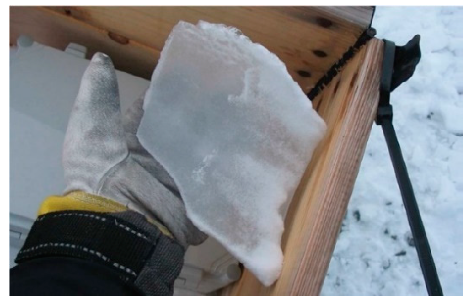
Risk 4. Thrown ice pieces from operational wind turbines (Ice throw): This phenomenon can occur when pieces of ice are either thrown away from an operational WT, see Figure 3, due to the aerodynamic and centrifugal forces, or dropped down if the WT was idle. In both cases, ice pieces landing on the ground will represent a hazard to the safety of the WF including the WTs, WF facilities, crew personnel, and animals [8]. A simple equation (Equation (3)) can be used to measure the distance of thrown ice pieces from an operational WT as follows [35]:
where (d) is the throwing distance, (D) is the rotor blade diameter, and (H) is the hub height.
d = 1.5 (D + H)

Figure 3.
Ice piece thrown from a WT in Arctic Norway WF [36]. Reprint with permission from author [Matthew Homola], 2022, NTNU Norwegian University of Science and Technology.
The probability of ice throw from operational WTs depends on the probability of ice formation on the WT blades, the probability of being thrown away to a location where ice pieces may represent a hazard to WF surroundings, and the probability of members of the public, crew personnel, and animals being present within the range of landing ice pieces [37]. The probability of ice accretion on WT blades depends on many factors such as the air temperature, wind speed, liquid water content (LWC), median volume diameter (MVD), and the elevation of WT from the sea level [38].
Rime ice and glaze ice are the two most common types of ice to accrete on the blades of WTs. Rime ice forms when supercooled water droplets freeze immediately upon impacting the surface of the blade, while glaze ice forms when the liquid water freezes shortly after impacting the surface of the blade [39]. Glaze ice accretion forms near the freezing point (0 °C) and has strong adhesion to the surface; it is transparent and has a higher density than rime ice. On the other hand, rime ice has lower adhesion to the surface and has a white or opaque color [40].
The probability of ice formation on WTs can be reflected by estimating the daily intensity of the icing events in kg/m2. Table 2 summarizes five site icing index categories that can be used to determine the intensity of icing on WTs in the WF location on a daily basis [41].

Table 2.
Site icing index categories.
Risk 5. Environmental risks: The Arctic, as an example of CCR, is known for its sensitive environment. Locating WFs in the Arctic will lead to possible impacts on the critical habitats and threatened species. For example, bird mortalities caused by WTs have been debatable [42] for several years, even though it is stated that wind energy killed 20 times fewer birds compared to fossil fuels, and the number of birds killed by WTs can be negligible compared to some other human activities [43]. In addition, the construction phase of wind farms might result in pollution of nearby surface or underground water [44]. Similarly, the use of liquids such as the gearbox lubricating oil might result in pollution in case it leaked from the WT. Moreover, the Arctic area is known for reindeer grazing, therefore, having WFs built on winter grazing areas for reindeer might affect their density, especially during the construction phase or even after it.
Risk 6. Social opposition: The visual presence of WTs can be annoying, especially to residents living nearby WFs. The presence of WFs might stop or limit the ability of local communities to utilize the surrounding lands and might affect its economy [45]. In addition, the generated noise by WTs might be annoying to residents living nearby WFs. The sources of the generated noise by WTs are the mechanical components such as the gearbox and control mechanisms, and the rotation of the WT blades through the air. Noise levels are measured by decibels (dB(A)), which is a scale designed to measure how the human ear perceives the sound frequencies. The day–evening–night noise level (Lden) is a European standard to express the noise levels from machines throughout an entire day [46]. The institution of occupational safety and health (IOSH) designed a scale for classifying noise levels [47], which can be used to assess the severity of noise emitted by WTs, as shown in Table 3.

Table 3.
Noise levels classification.
5. Probabilities of Risk Occurrence and Severity of Consequences Criteria
Table 4 determines the criteria for estimating the probability of each of the identified risks. The criteria are based on reviewed research studies, measured data, and human evidence. Selecting the probability level for each risk type is primarily dependent on the WT or WF under the study.

Table 4.
Criteria for the probabilities of risks experienced by WFs in CCRs.
Table 5 shows the criteria selected for measuring the consequences of the identified six risks. The consequences of risks are defined differently based on the type of risk being assessed. The consequences can be evaluated depending on the resulting system deterioration, injuries or loss of lives, maintenance delays, and short- or long-term effects.

Table 5.
Criteria for the consequences of risks experienced by WFs in CCRs.
6. Experts’ Judgments
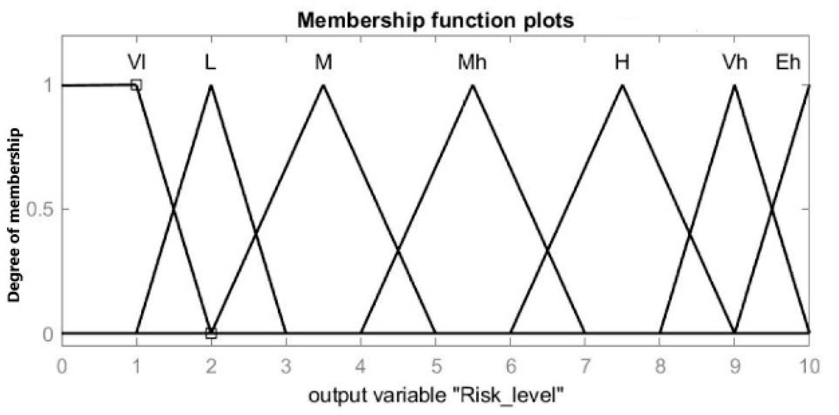
The preceding criteria were sent to seven experts, who were asked to provide their range of values for each fuzzy linguistic term used to assess the probability (Very low (Vl), Low, Medium, high, Very high (Vh)) and the consequences (Low, Moderate, High, Very high) term, as well as the risk levels, which are described as Very low (Vl), Low (L), Moderate (M), Moderate-high(MH), High(H), Very high (Vh), and Extremely high (Eh). Afterwards, the data gathered from the experts were used to design the membership functions that reflected these fuzzy terms.
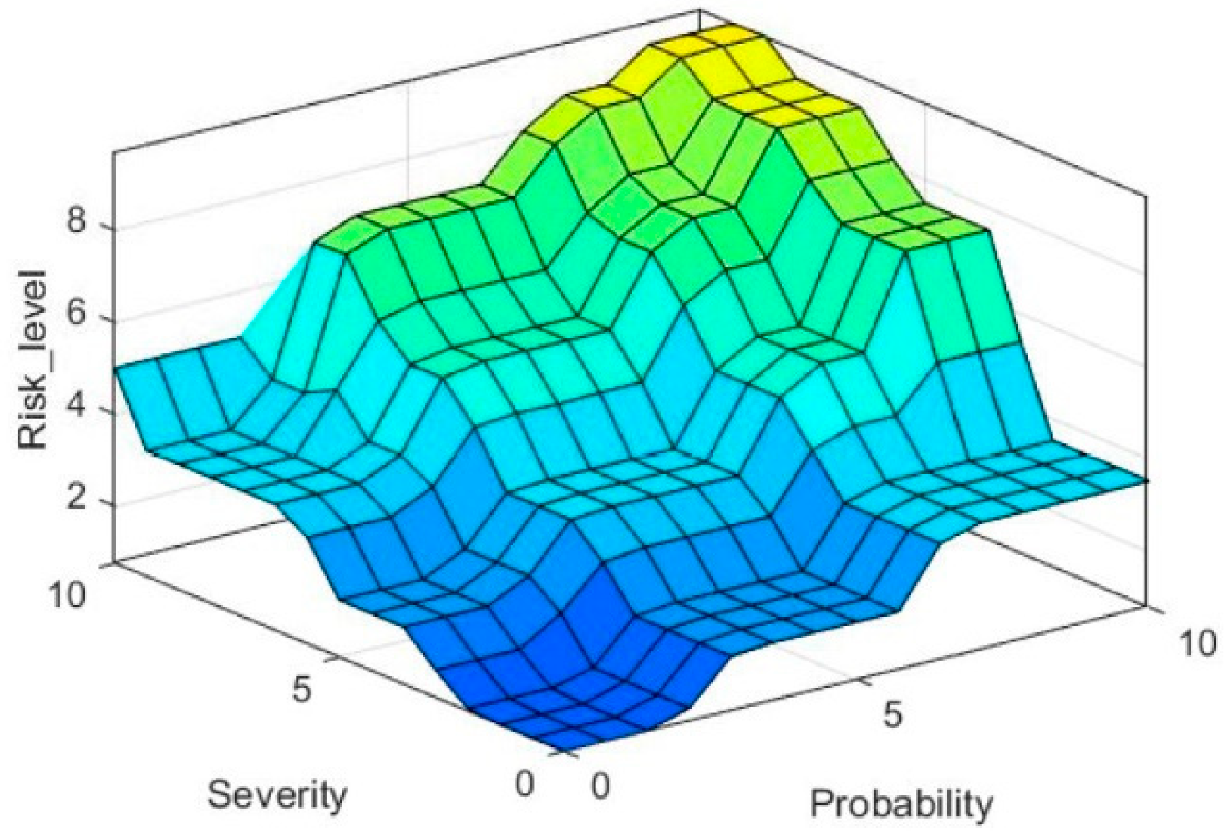
The selected experts have backgrounds ranging from university professors working on wind energy to experienced staff at wind farms in Arctic Norway. Experts were assumed to have equal weights for their answers. Based on the average values for the probabilities, consequences, and risk levels collected from the experts, and by using MATLAB fuzzy logic toolbox, the triangular membership functions for the input variables (i.e., probabilities and consequences) and the output variable (the risk levels) were defined, as shown in Figure 4 and Figure 5, where the x-axis represents the input values provided by the experts (from 0 to 10), and the y-axis represents the degree of membership (from 0 to 1) for each membership function. The combination between these three variables can be represented by a 3-dimensional surface plot, in Figure 6, which shows a fuzzy risk matrix.

Figure 4.
Membership functions of probabilities (a) and consequences (b) of risks based on experts’ judgments.

Figure 5.
The membership functions of risk levels based on experts’ judgments.

Figure 6.
Fuzzy risk matrix combining the three variables for risk analysis.
For more illustration, the y-axis in Figure 4a,b represents the degree to which a certain input (a probability or a consequence) can be described as low, medium, high, etc. For example, if the average value of the probability of a certain risk, given by experts, was 5, that means that the degree of membership of the probability of that risk is 80% medium, as per Figure 4a. Similarly, if the severity of a specific risk was determined by experts to be 9, that means that the severity of that risk is 100% very high, as per Figure 4b. Following that, the defined inference rules will determine the level of the risk in fuzzy terms. A logical inference rule that applies to this example can be: if the probability is medium and severity is very high, then risk level is high. The degree of membership of the risk level is determined using the minimum operator as in Equation (4) [20]:
where μ (Risk is high) is the degree of membership of the risk level as a high risk. Afterwards, the risk level is determined by referring to Figure 5, where the x-axis value for the risk level that corresponds to 80% high risk is equal to 7.5.
μ (Risk is high) = min (0.8; 1) = 0.8
The fuzzy inference functions in MATLAB used in this risk analysis application are shown in Table 6. The membership functions defined by the experts are used to generate the fuzzy rules that will be used to rank the risks. A total of 5×4 = 20 rules were generated. Examples of these rules are as follows:

Table 6.
MATLAB fuzzy inference functions used.
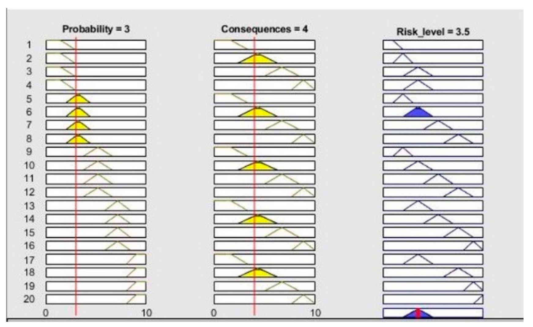
- Rule 1: If probability is very low and consequence is low, then the risk level is very low.
- Rule 11: If probability is medium and consequence is high, then the risk level is moderate-high.
- Rule 19: If probability is very high and consequence is high, then the risk level is very high.
A detailed description of the WF was sent to the experts, who were asked to provide their numeric values for the probabilities and consequences of each risk. Afterwards, the fuzzy logic toolbox in MATLAB was used to calculate the risk level using the centroid method [52]. Figure 7 illustrates the different probability and consequence combinations, based on the defined 20 fuzzy rules, to calculate the risk level values.
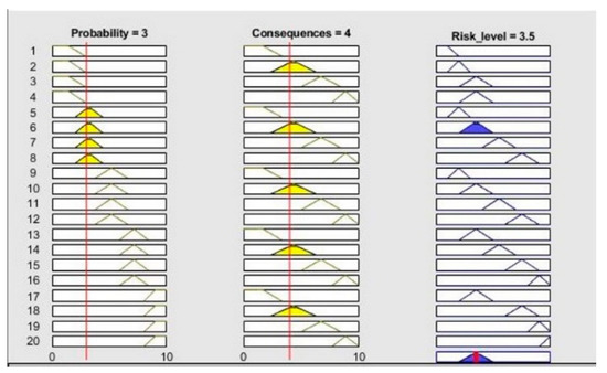
Figure 7.
Rules of probabilities and consequences for risk level calculation.
- Case Study: Wind farm in Arctic Norway
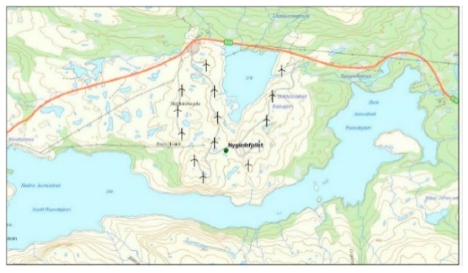
A WF in Arctic Norway, with a layout shown in Figure 8, was selected to demonstrate the proposed methodology. The selected WF is located in a valley at around 420 m above the sea level. The WF consists of fourteen 2.3 MW WTs. In order to support the experts in their estimations, operational and site specifications data about the WF were acquired from different sources. For example, data regarding failure rates, icing rates, maintenance reports, and WTs performance were acquired from the WF operator; this data covered two years of WF operation, from 2019 to 2020. In addition, data regarding the WF’s site specifications and weather data were acquired from published research articles and manufacturers’ technical publications, as well as weather stations that publish their data online.

Figure 8.
Wind farm location and layout.
6.1. Analysis
MATLAB fuzzy logic toolbox was utilized to calculate the level of each risk on the basis of the average values of the probabilities and consequences of each risk provided by the experts. Table 7 shows the average probability and consequence values determined by the experts as well as the resulting risk level calculated by MATLAB. In addition, the table shows the ranking of the risks, where limited accessibility to WF risk is assigned the highest rank (1), and social opposition risk is assigned the lowest rank (6).

Table 7.
Ranking of risks considering average values of probabilities, consequences, and risk levels.
Risk 1 (WT stoppage). From the data gathered from the WF operator, there were 1993 stoppages experienced by the WTs during 2019, mainly due to maintenance. In addition, December 2019 was the month that witnessed the highest rate of WT stoppages due to icing, which was 65 stoppages. Equation (1) was applied separately to determine the probability of stoppage per WT per month due to failure and per month due to icing. It was found out that the probability of stoppage was 29% per WT per month. Those stoppages did not result in deterioration of the WF production and operation was resumed as regular, according to the WF operator.
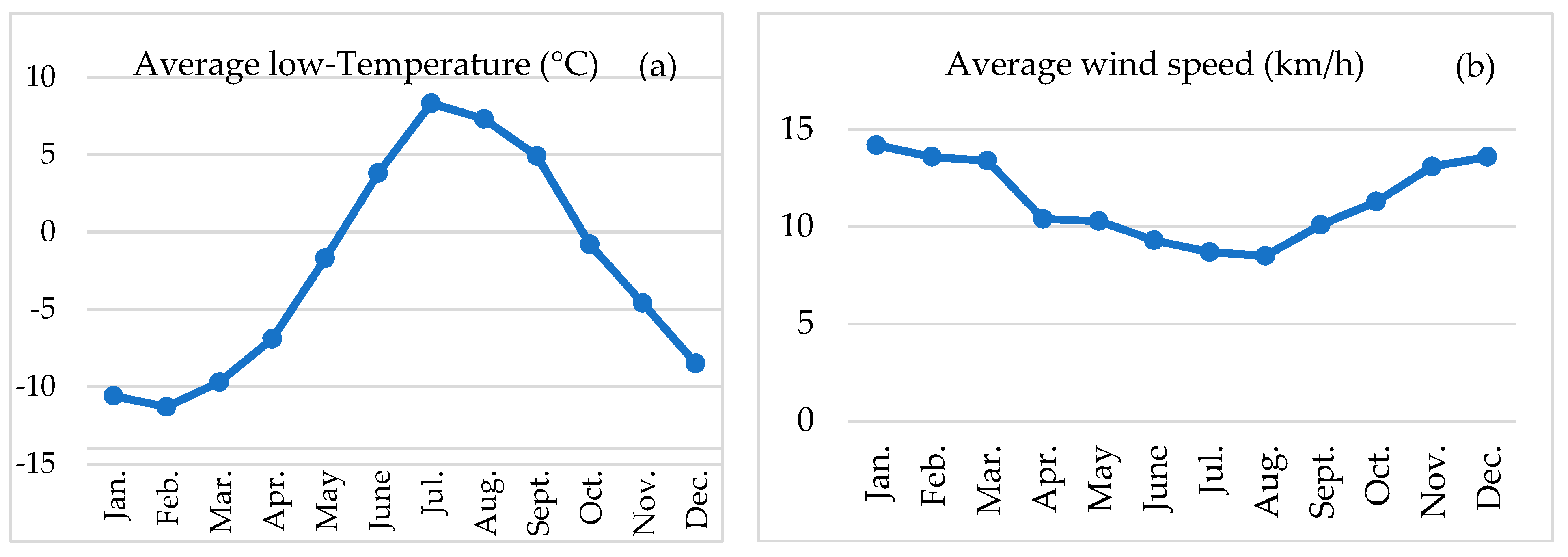
Risk 2 (Cold stress). The coldest average ambient temperatures impacting the WF occur during January, February, and March, according to Figure 9a, with the coldest average temperature of as low as nearly −12 °C recorded in February. In addition, the average monthly wind speed during the same month is 13.6 km/h, as shown in Figure 9b [53]. By applying Equation (2), the WCT during February is calculated to be about −19 °C, which indicates no risk of frostbite to workers at the WF. In addition, according to the WF operator, there are no injuries recorded or illnesses caused to workers at the WF by very cold WCTs.
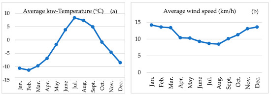
Figure 9.
Monthly average temperatures (a) and wind speeds (b) at the WF’s location [54]. Data were gathered from Weather Atlas.
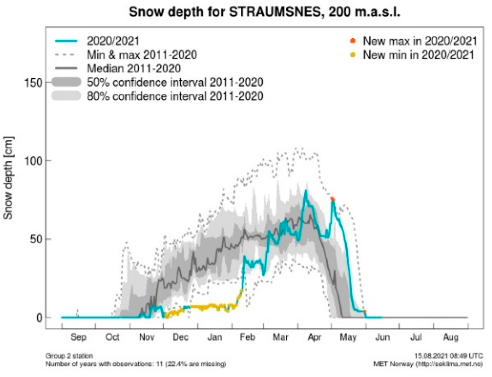
Risk 3 (Limited accessibility). The Norwegian Meteorological Institute [55] provides information about the snow depth of specific sites in Norway through weather stations distributed in different areas of the country. The closest weather station to the WF is located in Straumsnes. Figure 10 shows that the highest recorded snow depth in 2020 occurred during February until May, with a maximum snow depth of 75 cm recorded in April. Such accumulation of snow requires specially equipped vehicles, such as snowcats and snowmobiles to be available all the time, to maintain access to the WF under severe weather conditions, which was confirmed by the WF operator during a visit to the WF by the authors. Besides that, during periods of peak snow accumulation, snow removal strategies are implemented, which can be costly [4].

Figure 10.
Snow depth in an area close to the WF [55].
Risk 4 (Ice throw). A field study shows that the daily intensity of icing in Narvik, a city close to the WF, is approximately 14.5–18.5 kg/m2 during January, February, and March, as shown in Figure 11 [56]; those measurements can be assumed close enough to be applicable to the site under consideration. This indicates a light icing intensity with site icing index for the WF site, according to Table 1. By applying Equation (3) to calculate the throwing distance of ice pieces, it is found that the throwing distance is 255 m. The closest residential area to the WF is kilometers away. Moreover, a main road passes next to the WF, but it is around 500 m away from the closest WT, which means that no residents or personnel exist within the range of ice throw risk.
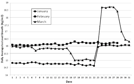
Figure 11.
Icing intensity close to the WF site during January, February, and March [56]. Reprint with permission from author [Muhammad S. Virk], 2022, The International Journal of Ocean and Climate Systems.
Risk 5 (Environmental risks). A study by Jacobsen et.al. [57] revealed that the number of registered birds migrating through the WF area was low, where the average number of observed birds passing through the WF was around five birds during 4 h of observation in a day. This is primarily due to the topography and local conditions of that area, which is not inviting to migrating birds. However, the area around the WF has great value for reindeer husbandry and is used for reindeer grazing during autumn and winter. In this respect, field results show that the density of reindeer in WF areas in Arctic Norway do not change significantly, and that reindeer can adapt and keep using WF areas for grazing [58]. With regards to environmental pollution, there is no evidence that the WF caused pollution to nearby waters or to the environment in general.
Risk 6 (Social opposition). The presence of the WTs and the noise they generate are not expected to cause annoyance to humans due to the fact that the WF is located away from residential areas, in a valley with surrounding mountains as high as 2000 m above sea level from the north and south. Besides, the location of the WF is not classified as a touristic area. However, there is a main road that passes next to the WF, which means that drivers and passengers passing by the WF will be subjected to this noise level for very short time. According to one study, the level of noise generated by a similar WT located at approximately 500 m far, which is nearly the distance between the closest WT and the main road, would be 48 dB(A) at a wind speed of 10 m/s [59], meaning that the noise severity can be described as low.
6.2. A Wind Farm under Normal Operating Conditions
In order to compare the effects of cold climate operating conditions on the calculated risk level and ranking of risks, the same methodology is applied to a WF located in a non-cold-climate region. The Kozbeyli WF [45], in Turkey has higher reliability, with lower rate of WT stoppages, no ice accretion on the blades of the WTs, less snow accumulation on the roads of the WF, and a 3.1 km access road built to guarantee access to the WF. However, the WF is close to an Environmentally Protected Area in Foça, with a bird migration route 4 km to the south of the WF [60]. Moreover, in the WF area, there are endangered species such as Passer Domesticus and Crocidura Russula, that were identified and listed by the Bern Convention [45].
Furthermore, the WF is located 1.3 km near to a touristic village, which has natural and historical values. Social acceptance of the WF was determined to be poor due to its impact on tourism in that area. Based on the preceding information, Table 8 demonstrates the ranking of risks using experts’ judgments and MATLAB fuzzy logic toolbox. It can be seen from the table that the social opposition risk ranked the highest, followed by the environmental risks, while the risk of ice throw from WTs ranked as the lowest risk, flowed by the risk of WT stoppage.

Table 8.
Ranking of risks for the Kozbeyli WF in Turkey using experts’ judgments and fuzzy logic.
7. Conclusions
In this paper, six types of risks that are related to the operation of WFs in CCRs. These risks were distinguished as being caused by the harsh weather conditions, and risks caused by the WFs on their surrounding environment and community. The identified risks were analyzed using expert judgment and MATLAB fuzzy logic toolbox. The identified risks are the increased WT stoppages risk, cold stress to workers risk, limited accessibility to WFs risk due to snow accumulations on the roads, ice throw from WTs risk, environmental risks, and social opposition risk.
Based on a research review, gathered data, and published data, and experts’ reasoning, two criteria tables were defined for the probability of occurrence and the severity of consequences of each risk. Furthermore, experts’ judgments and MATLAB fuzzy logic toolbox were used to graph the membership functions for the probabilities and consequences of each risk (the inputs), as well as risk levels (the output). The risk levels were calculated based on a set of 20 rules generated using the experts’ data.
A WF in Arctic Norway was selected to illustrate the proposed methodology. Experts were provided with a description of the WF and were asked to deliver their assessed values for the probabilities and consequences of each risk. Through the calculated risk level, it was concluded that limited accessibility to the WF ranked as the highest risk, followed by WT stoppage. On the other hand, social opposition was ranked as the lowest risk followed by the ice throw.
In order to demonstrate the methodology further, a WF that is not subjected to cold climate operating conditions, located in Turkey, was selected. The social opposition to the WF was ranked as the highest risk followed by the environmental risks, where the ice throw risk and WT stoppage risk were deemed to be the lowest-ranked risks. This was due to the fact that the Turkish WF was installed close to a village with touristic value and in a area that is a home for endangered species.
Author Contributions
A.M.M. developed the methodology, conducted the literature review, and gathered the data to establish the probabilities and consequences criteria, gathered the data from the experts, performed the risk analysis using MATLAB fuzzy logic toolbox, and wrote the paper; A.B., as a main supervisor, followed up all study steps and gave helpful guidance and reviewed and edited the manuscript. All authors have read and agreed to the published version of the manuscript.
Funding
This research received no external funding.
Data Availability Statement
The data gathered from the wind farm are subjected to a non-disclosure agreement. Therefore, an approval from the wind farm is required in case the data are needed. The data gathered from the experts can be provided upon request from the editors.
Conflicts of Interest
The authors announce no conflict of interest.
Nomenclature
| WT | Wind turbine |
| WF | Wind farm |
| CCR | Cold climate region |
| X | Universal set |
| A | A fuzzy subset |
| μ(x) | Membership function |
| λ | Stoppage rate per wind turbine per year |
| Lden | day–evening–night noise level |
| WCT | Wind chill temperature |
| V | Wind speed (km/h) |
| T | Air temperature (°C) |
| P | probability |
| dB(A) | decibels |
| IOSH | The institution of occupational safety and health |
References
- GWEC. Global Wind Report. Annual Market Update 2010; Springer: Berlin, Germany, 2011; Volume 1, pp. 12–20. [Google Scholar]
- Fortin, G.; Perron, J.; Ilinca, A. Behaviour and modeling of cup anemometers under Icing conditions. In Proceedings of the International Workshop on Atmospheric Icing of Structures (IWAIS XI), Montréal, QC, Canada, 13–16 June 2005. [Google Scholar]
- Fossem, A.A. Short-Term Wind Power Prediction Models in Complex Terrain Based on Statistical Time Series Analysis. Master’s Thesis, UiT The Arctic University of Norway, Tromso, Norway, 2019. [Google Scholar]
- Lehtomäki, V. Available Technologies for Wind Energy in Cold Climates, Sweden. 2018. Available online: https://iea-wind.org/task19/ (accessed on 12 August 2021).
- Afzal, F.; Virk, M.S. Review of icing effects on wind turbine in cold regions. E3S Web Conf. 2018, 72, 01007. [Google Scholar] [CrossRef] [Green Version]
- Naseri, M.; Fuqing, Y.; Barabady, J. Performance-based aggregation of expert opinions for reliability prediction of Arctic offshore facilities. In Proceedings of the 2015 IEEE International Conference on Industrial Engineering and Engineering Management (IEEM), Singapore, 6–9 December 2015. [Google Scholar]
- Mustafa, A.M.; Barabadi, A.; Markeset, T.; Naseri, M. An overall performance index for wind farms: A case study in Norway Arctic region. Int. J. Syst. Assur. Eng. Manag. 2021, 12, 938–950. [Google Scholar] [CrossRef]
- Mustafa, A.M.; Barabadi, A.; Markeset, T. Risk assessment of wind farm development in ice proven area. In Proceedings of the 25th International Conference on Port and Ocean Engineering under Arctic Conditions (POAC), Delft, The Netherlands, 9–13 June 2019. [Google Scholar]
- Enevoldsen, P. Onshore wind energy in Northern European forests: Reviewing the risks. Renew. Sustain. Energy Rev. 2016, 60, 1251–1262. [Google Scholar] [CrossRef]
- ISO 31000; Risk Management—Principles and Guidelines. International Standardization Organization: Cham, Switzerland, 2018.
- Chehouri, A.; Younes, R.; Ilinca, A.; Perron, J. Review of performance optimization techniques applied to wind turbines. Appl. Energy 2015, 142, 361–388. [Google Scholar] [CrossRef]
- Shourangiz-Haghighi, A.; Haghnegahdar, M.A.; Wang, L.; Mussetta, M.; Kolios, A.; Lander, M. State of the art in the optimisation of wind turbine performance using CFD. Arch. Comput. Methods Eng. 2020, 27, 413–431. [Google Scholar] [CrossRef]
- Carrillo, C.; Montaño, A.O.; Cidrás, J.; Díaz-Dorado, E. Review of power curve modelling for wind turbines. Renew. Sustain. Energy Rev. 2013, 21, 572–581. [Google Scholar] [CrossRef]
- Lydia, M.; Kumar, S.; Selvakumar, A.I.; Kumar, G.E.P. A comprehensive review on wind turbine power curve modeling techniques. Renew. Sustain. Energy Rev. 2014, 30, 452–460. [Google Scholar] [CrossRef]
- Bai, C.-J.; Wang, W.-C. Review of computational and experimental approaches to analysis of aerodynamic performance in horizontal-axis wind turbines (HAWTs). Renew. Sustain. Energy Rev. 2016, 63, 506–519. [Google Scholar] [CrossRef]
- Fakorede, O.; Feger, Z.; Ibrahim, H.; Ilinca, A.; Perron, J.; Masson, C. Ice protection systems for wind turbines in cold climate: Characteristics, comparisons and analysis. Renew. Sustain. Energy Rev. 2016, 65, 662–675. [Google Scholar] [CrossRef]
- Luengo, M.M.; Kolios, A. Failure mode identification and end of life scenarios of offshore wind turbines: A review. Energies 2015, 8, 8339–8354. [Google Scholar] [CrossRef] [Green Version]
- Leimeister, M.; Kolios, A. A review of reliability-based methods for risk analysis and their application in the offshore wind industry. Renew. Sustain. Energy Rev. 2018, 91, 1065–1076. [Google Scholar] [CrossRef]
- Gallab, M.; Bouloiz, H.; Alaoui, Y.L.; Tkiouat, M. Risk assessment of maintenance activities using fuzzy logic. Procedia Comput. Sci. 2019, 148, 226–235. [Google Scholar] [CrossRef]
- Pokoradi, L. Fuzzy logic-based risk assessment. Acad. Appl. Res. Mil. Sci. 2002, 1, 63–73. [Google Scholar]
- Dinmohammadi, F.; Shafiee, M. A fuzzy-FMEA risk assessment approach for offshore wind turbines. Int. J. Progn. Health Manag. 2013, 4, 59–68. [Google Scholar] [CrossRef]
- Peng, Y.; Asgarpoor, S.; Qiao, W.; Foruzan, E. Fuzzy cost-based FMECA for wind turbines considering condition monitoring systems. In Proceedings of the North American Power Symposium (NAPS), Denver, CO, USA, 18–20 September 2016. [Google Scholar]
- Markowski, A.S.; Mannan, M.S. Fuzzy logic for piping risk assessment (pfLOPA). J. Loss Prev. Process Ind. 2009, 22, 921–927. [Google Scholar] [CrossRef]
- Yang, Z.; Wang, J. Use of fuzzy risk assessment in FMEA of offshore engineering systems. Ocean Eng. 2015, 95, 195–204. [Google Scholar] [CrossRef]
- Zadeh, L.A. Fuzzy sets. In Fuzzy Sets, Fuzzy Logic, and Fuzzy Systems: Selected Papers; World Scientific: Singapore, 1996; pp. 394–432. [Google Scholar]
- Dernoncourt, F. Introduction to Fuzzy Logic; Massachusetts Institute of Technology: Cambridge, MA, USA, 2013; p. 21. [Google Scholar]
- Mamdani, E.H.; Assilian, S. An experiment in linguistic synthesis with a fuzzy logic controller. Int. J. Man Mach. Stud. 1975, 7, 1–13. [Google Scholar] [CrossRef]
- Sari, W.E.; Wahyunggoro, O.; Fauziati, S. A comparative study on fuzzy Mamdani-Sugeno-Tsukamoto for the childhood tuberculosis diagnosis. AIP Conf. Proc. 2016, 1755, 070003. [Google Scholar]
- Barabadi, A.; Garmabaki, A.; Zaki, R. Designing for performability: An icing risk index for Arctic offshore. Cold Reg. Sci. Technol. 2016, 124, 77–86. [Google Scholar] [CrossRef]
- Peltola, E.; Laakso, T.; Ronsten, G.; Tallhaug, L.; Horbaty, R.; Baring-Gould, I.; Lacroix, A. Wind energy projects in cold climates. Int. Energy Agency 2005, 36, 12–13. [Google Scholar]
- Andersen, E.; Börjesson, E.; Vainionpää, P.; Undem, L.S. Wind Power in Cold Climate Report; WSP-Environmental: Oslo, Norway, 2011; Available online: https://www.diva-portal.org/smash/get/diva2:707416/FULLTEXT01.pdf (accessed on 11 May 2019).
- Mustafa, A.M.; Barabadi, A. Resilience Assessment of Wind Farms in the Arctic with the Application of Bayesian Networks. Energies 2021, 14, 4439. [Google Scholar] [CrossRef]
- Wærø, I.; Rosness, R.; Skaufel Kilskar, S. Human Performance and Safety in Arctic Environments; SINTEF: Trondeheim, Norway, 2018. [Google Scholar]
- Osczevski, R.; Bluestein, M. The new wind chill equivalent temperature chart. Bull. Am. Meteorol. Soc. 2005, 86, 1453–1458. [Google Scholar] [CrossRef] [Green Version]
- Seifert, H.; Westerhellweg, A.; Kröning, J. Risk analysis of ice throw from wind turbines. Boreas 2003, 6, 2006-01. [Google Scholar]
- Homola, M.C. Atmospheric Icing on Wind Turbines: Modeling and Consequences for Energy Production. Ph.D. Thesis, Norwegian University of Science and Technology, Trondheim, Norway, 2011. [Google Scholar]
- LeBlanc, M.P.; Morgan, C.A.; Bossanyi, E.A.; Garrad, A.D. Recommendations for Risk Assessments of Ice Throw and Blade Failure in Ontario; Garrard Hassan Canada Inc.: Montreal, QC, Canada, 2007. [Google Scholar]
- Ingvaldsen, K. Atmospheric Icing in a Changing Climate. Master’s Thesis, Department of Geosciences, Faculty of Mathematics and Natural Sciences, University of Oslo, Oslo, Norway, 2017. [Google Scholar]
- Bravo Jimenez, I. Detection and Removal of Wind Turbine Ice: Method Review and a CFD Simulation Test. Ph.D. Thesis, University of Gävle, Gävle, Sweden, 2018. [Google Scholar]
- Xue, H.; Khawaja, H. Review of the phenomenon of ice shedding from wind turbine blades. Int. J. Multiphys. 2016, 10, 265–276. [Google Scholar]
- Fikke, S.M.; Ronsten, G.; Heimo, A.; Kunz, S.; Ostrozlik, M.; Persson, P.E.; Sabata, J.; Wareing, B.; Wichura, B.; Chum, J.; et al. COST 727: Atmospheric Icing on Structures: Measurements and Data Collection on Icing: State of the Art. 2006. Available online: https://www.researchgate.net/publication/263529195_COST-727_Atmospheric_Icing_on_Structures_Measurements_and_Data_Collection_on_Icing_State_of_the_Art (accessed on 20 December 2021).
- Aishwarya, K.; Kathryn, J.C.; Lakshmi, R.B. A survey on bird activity monitoring and collision avoidance techniques in windmill turbines. In 2016 IEEE Technological Innovations in ICT for Agriculture and Rural Development (TIAR); IEEE: Piscataway, NJ, USA, 2016; pp. 188–193. [Google Scholar]
- Sovacool, B.K. Contextualizing avian mortality: A preliminary appraisal of bird and bat fatalities from wind, fossil-fuel, and nuclear electricity. Energy Policy 2009, 37, 2241–2248. [Google Scholar] [CrossRef]
- Lu, J.; Bui, M.T.; Yuan, F. Evaluation of the water quality at Bogdalen watershed near Kvitfjell and Raudfjell wind farm area. IOP Conf. Ser. Earth Environ. Sci. 2019, 344, 012022. [Google Scholar] [CrossRef]
- Kucukali, S. Risk scorecard concept in wind energy projects: An integrated approach. Renew. Sustain. Energy Rev. 2016, 56, 975–987. [Google Scholar] [CrossRef]
- Przysucha, B.; Pawlik, P.; Stępień, B.; Surowiec, A. Impact of the noise indicators components correlation Ld, Le, Ln on the uncertainty of the long-term day–evening–night noise indicator Lden. Measurement 2021, 179, 109399. [Google Scholar] [CrossRef]
- The Institution of Occupational Safety and Health. Noise—Typical and Hazardous Noise Levels. 2018. Available online: https://iosh.com/resources-and-research/our-resources/occupational-health-toolkit/noise/typical-and-hazardous-noise-levels/ (accessed on 20 January 2022).
- Spinato, F.; Tavner, P.; van Bussel, G.; Koutoulakos, E. Reliability of wind turbine subassemblies. IET Renew. Power Gener. 2009, 3, 387–401. [Google Scholar] [CrossRef] [Green Version]
- Nordlysvind. Kvitfjell/Raudfjell Project Information. 2018. Available online: https://nordlysvind.no/project-information/environment/?lang=en (accessed on 14 August 2021).
- Mohr, R. Preliminary Hazard Analysis; Jacobs Sverdrup.: Tullahoma, TN, USA, 2002. [Google Scholar]
- Anand, P.; Ceylan, H.; Gkritza, K.; Talor, P.; Pyrialakou, V.; Kim, S.; Gopalakrishnan, K. Cost Comparison of Alternative Airfield Snow Removal Methodologies. 2014. Available online: https://works.bepress.com/halil_ceylan/223/ (accessed on 2 December 2021).
- Cheng, C.-H. A new approach for ranking fuzzy numbers by distance method. Fuzzy Sets Syst. 1998, 95, 307–317. [Google Scholar] [CrossRef]
- Atlas, W. Monthly Weather Forecast and Climate Narvik, Norway. 2022. Available online: https://www.weather-atlas.com/en/norway/narvik-climate#climate_text_1 (accessed on 20 January 2022).
- Sundina, E.; Makkonen, L. Ice Loads on a Lattice Tower Estimated by Weather Station Data. J. Appl. Meteorol. 1998, 37, 523–529. [Google Scholar] [CrossRef]
- Norwegian Meteorological Institute. Snow Depth in Straumsnes. 2021. Available online: https://cryo.met.no/sites/cryo.met.no/files/latest/snowdepth_84500_latest_en.png (accessed on 15 August 2021).
- Rashid, T.; Mughal, U.N.; Mustafa, M.Y.; Virk, M.S. A field study of atmospheric icing analysis in a complex terrain of the high north. Int. J. Ocean Clim. Syst. 2014, 5, 189–197. [Google Scholar] [CrossRef]
- Jacobsen, K.-O. Nygårdsfjellet Vindpark, Trinn 2. Undersøkelser av Vårtrekk for Fugl. NINA Rapport. 2007. Available online: https://brage.nina.no/nina-xmlui/handle/11250/2455384 (accessed on 2 December 2021).
- Tsegaye, D.; Colman, J.E.; Eftestøl, S.; Flydal, K.; Røthe, G.; Rapp, K. Reindeer spatial use before, during and after construction of a wind farm. Appl. Anim. Behav. Sci. 2017, 195, 103–111. [Google Scholar] [CrossRef] [Green Version]
- Smith, A.C.; Wanka, K.M. Noise Assessment: Hermosa West Wind Farm Project; Wind Energy: Houston, TX, USA, 2010. [Google Scholar]
- Hämäläinen, R.; Kettunen, E.; Marttunen, M.; Ehtamo, H. Evaluating a framework for multi-stakeholder decision support in water resources management. Group Decis. Negot. 2001, 10, 331–353. [Google Scholar] [CrossRef]
Publisher’s Note: MDPI stays neutral with regard to jurisdictional claims in published maps and institutional affiliations. |
© 2022 by the authors. Licensee MDPI, Basel, Switzerland. This article is an open access article distributed under the terms and conditions of the Creative Commons Attribution (CC BY) license (https://creativecommons.org/licenses/by/4.0/).

