Abstract
The present research article focuses on an analytically based method for the optimal allocation and sizing of a renewable energy source (RES) capable of injecting both active and reactive powers in the distribution network. The placement of distributed generation (DG) in the distribution network reduces the magnitude of branch current in between the reference bus and the bus where DG is to be installed. Due to this, system power loss decreases significantly. The proposed method considers different levels of load in addition to peak load demand. The goal of the developed method is to minimize system losses by optimal DG allocations. In the proposed method, the optimum size of the DG is obtained on the basis of maximum loss saving criterion. For the execution of proposed method, only a base case load flow solution is required. The developed method has been tested on IEEE 69-bus and 33-bus radial distribution networks. On the basis of obtained results, it has been realized that the developed method is more capable of diminishing system energy losses.
1. Introduction
Exponential increase in electricity demand, continuous depletion of conventional power resources, environmental issues, uncertainties related to fuel prices and advances in DG technologies have motivated the power system planner to use small-scale generation units. A small-scale, electrical power generation unit is termed as DG. Further, DGs can be defined as the electricity-generating systems which are connected to customer side of the meter or load directly [1].
Moreover, DGs are beneficial when these DGs are integrated in the existing distribution network if allocation and sizing is performed in a strategic mode. Optimal sizing and siting of DG resources leads to decreased system power, energy loss along with system cost, and also enhances system bus voltage considerably. Further, optimally placed and sized DGs improve the voltage stability margin, loadability, quality of power and system reliability [1,2,3,4,5,6,7,8,9,10,11,12,13,14,15,16,17,18,19,20,21,22,23,24,25,26,27,28]. Moreover, DGs are driven by renewable energy sources and have the property of low emission of greenhouse gases (GHG) which are mainly responsible for global warming [1,4,13,15,16,17,18,22,23,26].
Non-optimally placed and sized DGs give rise to upsurges in system energy and power loss, increase system cost and enhance the profile of voltage in various load buses. Consequently, system performance deteriorates [4,13,18,19]. Therefore, optimum siting and sizing of DG units is a significant aspect and needs to be further investigated.
Many researchers investigated optimum sizing and siting of DGs as an objective to reduce system power and energy loss [2,3,4,5,6,7,8,9,10,11,12,13,14,15,16,17,18,19,20,21,22,23,24,25,26,27], voltage profile enhancement [2,3,4,5,6,7,8,10,18,19]. References [8,15,17,19,23,25,26] have addressed the betterment of the voltage stability margin (VSM), loadability of the system and system energy loss reduction as a single and multi-objective. Further, [2,3,4,6,7,8,9,10] have developed analytical methods for optimum siting and sizing of DG. References [5,24] addressed mixed integer non-linear programming (MINLP)-based methods, authors of [5,8,15,16,19,22,25] highlighted index-based methods, and evolutionary algorithms (EA) techniques have been applied by [11,18] for the solution and development of formulations. Reference [20] addressed the improvement of system reliability with the placement of DG.
In [2], authors have developed a technique based on an exact loss formula for the optimization of DG sizes and placement; authors derived analytical method-based formulations for the minimization of system power loss. Authors also examined the effect of DG size on system loss. References [3,4] developed a methodology for the optimal siting and sizing of renewable energy sources (RES) to decrease system active power loss on analytical method-based expressions. Wang and Nehrir [6] highlighted an analytically based technique for the siting of a single DG unit injecting real power into the system for mesh and radial distribution networks to reduce system losses. The authors considered different types of loads, but the optimum size of DG was not considered. The authors of [7] developed a loss sensitivity index based on analytical expressions and eliminate the need of the formation of a Jacobin matrix for optimum size and location of a single DG unit to minimize system power loss.
Hung and Mithulananthan [8] extended the similar technique as in [10] to the optimal installation of multiple DG units to reduce system power loss. In [9] authors have applied analytical formulations for optimal capacity and installation of renewable DGs to reduce the power loss of systems using a combination of time-varying load and different outputs from DG units. Further, Hung et al. [10] developed an improved analytical (IA)-based method for the optimum sizing and installation of different types of single DG units for loss reduction. In [11] authors have proposed a method for the optimal integration of non-dispatchable DG; the method is based on evolutionary programming. Hung et al. [12] applied an analytical formulation based on the multi-objective index for solar photovoltaic-based DGs for minimizing energy loss and the improvement of system voltage stability with time-varying load. Kansal et al. [14] highlighted the classification of different types of DGs which are operated by a non-conventional energy source such as biomass, solar and wind to decrease power loss via the optimal placement and sizing of DG. Murty and Kumar [15,16] proposed a new index method based on the power loss sensitivity factor and power stability for the optimal siting of DG units to reduce the energy loss cost of systems. In [17] authors have highlighted an analytically based method for optimum capacity and integration of both non-dispatchable and dispatchable DGs to minimize the system loss. Esmaili [18,19] addressed a method for optimum sizing and siting of DG to enhance system voltage stability and reduce system loss. Tah and Das [21] proposed new analytical formulations for optimal siting and sizing of DG for the minimization of system loss. Aman et al. [22,26] and Al Abri et al. [23] proposed a power stability index-based methodology for the optimum siting of DGs to reduce network power loss and enhance the voltage of bus. Ochoa and Harrison [25] addressed a new method for the optimal siting and sizing of DG to reduce energy loss of system. Mehta et al. [27] proposed a technique which is based on analytical formulations for the optimal selection, size and installation of different categories of DGs using the voltage sensitivity index method. Tawfeek et al. [28] proposed an exact loss formula based the analytical technique for the optimal allocation of DG and compared the results with PSO-based optimization techniques. The data of IEEE bus systems under investigation in the present study has been taken from [24]
In the proposed technique, system energy loss and energy loss saving formulations with DG and without DG have been derived in terms of D matrix. The process of formation of D matrix has been explained in Appendix A. Further, in earlier research papers, only peak load demand has been considered. Additionally, in the present study, three different levels of load demand have been considered. Moreover, as per available literature, the majority of the power system planners have developed expressions of DGs on exact loss formula-based analytical derivations [2,7,8,9,10,15,28] which are applicable for multiple and single DG unit(s) sizing and placement. The exact loss formula-based methodology requires the formation and calculation of an admittance (YBUS) matrix for solution of load flow equations which is a time-consuming process.
Moreover, due to the high R/X ratio and negligible shunt admittance of distribution lines, the conventional method of load flow, i.e., the Newton-Raphson and Gauss-Seidel methods, are not very suitable because of the convergence problem of these techniques. In the proposed paper the backward–forward sweep (BFS)-based method for load flow solution has been applied. The BFS-based method does not require the formation of a (YBUS) matrix, therefore the method has an excellent convergence property [2,3,4,5,7,9]. The present research article aims to estimate the optimal sizes and locations of DGs so that system energy losses could be reduced.
Further, the methods which appeared in the literature are suitable for passive networks; in such circuits a voltage issue is exposed due to variation in load demand. Therefore, in the present study, load demand is considered in different load levels.
Basically, the addition of DG units in distribution network changes the power flow which in turn changes the magnitude of branch current components (active and reactive); due to this system power losses are reduced. The candidate bus for DG placement are obtained on the basis of maximum loss saving criterion.
Furthermore, the developed technique needs solutions of base case load flow only for small as well as larger networks. The present technique has been applied to IEEE 69-bus and 33-bus and 85-bus radial distribution systems. Further, the results obtained by the present developed method are immensely encouraging for system energy loss minimization and the enhancement of system voltage profile view point.
In the proposed method, type 2 DGs have been considered for placement. This category of DG injects powers, i.e., active power and reactive power. In [18] authors proposed a bifurcation-based method to place the optimum number of DGs by finding the vulnerable buses, and these buses are found on the basis of voltage stability criteria. Beside the above explanation, a summary of the related work is represented in Table A1.
In the above-mentioned literature review, it is clear that very few authors addressed the analytical-based method, which is described in the present research article. In the present method, expressions of the optimum capacity of DGs are derived on the basis of maximum loss saving criterion. In the proposed method, sequence of buses is found on the basis of maximum power loss saving. The suitability of the proposed method is also checked and matching with available literature. Therefore, the current method is a novel analytically based method for the optimum capacity and integration of DGs (single as well as multiple DG units) in a distribution system. The computation time of the proposed method is very low, i.e., 10 s to 12 s, as it does not require the solution and formation of a Jacobian matrix.
The present paper is arranged in 5 sections: Section 2 describes the proposed methodology and mathematical formulation. Section 3 explains the algorithm for a solution, and Section 4 highlights the discussions along with results. Lastly, Section 5 describes conclusions and represents Appendix A.
2. Proposed Methodology and Mathematical Formulation
The following assumptions are made to the mathematical formulations of the developed analytically based method:
- The system under consideration is balanced, radial and fed by a substation.
- Voltage of all nodes is close to 1 p.u.
- The Shunt admittances of lines are negligible.
- Bus loads are modeled as a constant power load.
- The maximum capacity of DG for various test systems does not exceed the total connected load.
- The present paper investigates the optimal placement and sizing of such DG which is capable of delivering both active and reactive power. The flow diagram of the proposed approach is shown in Figure 1.
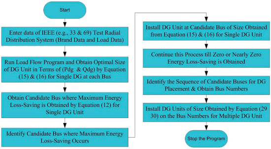 Figure 1. Proposed Approach for Optimal Integration of Renewable Energy Sources in Distribution Systems.
2.1. Mathematical Formulations for Single DG Unit
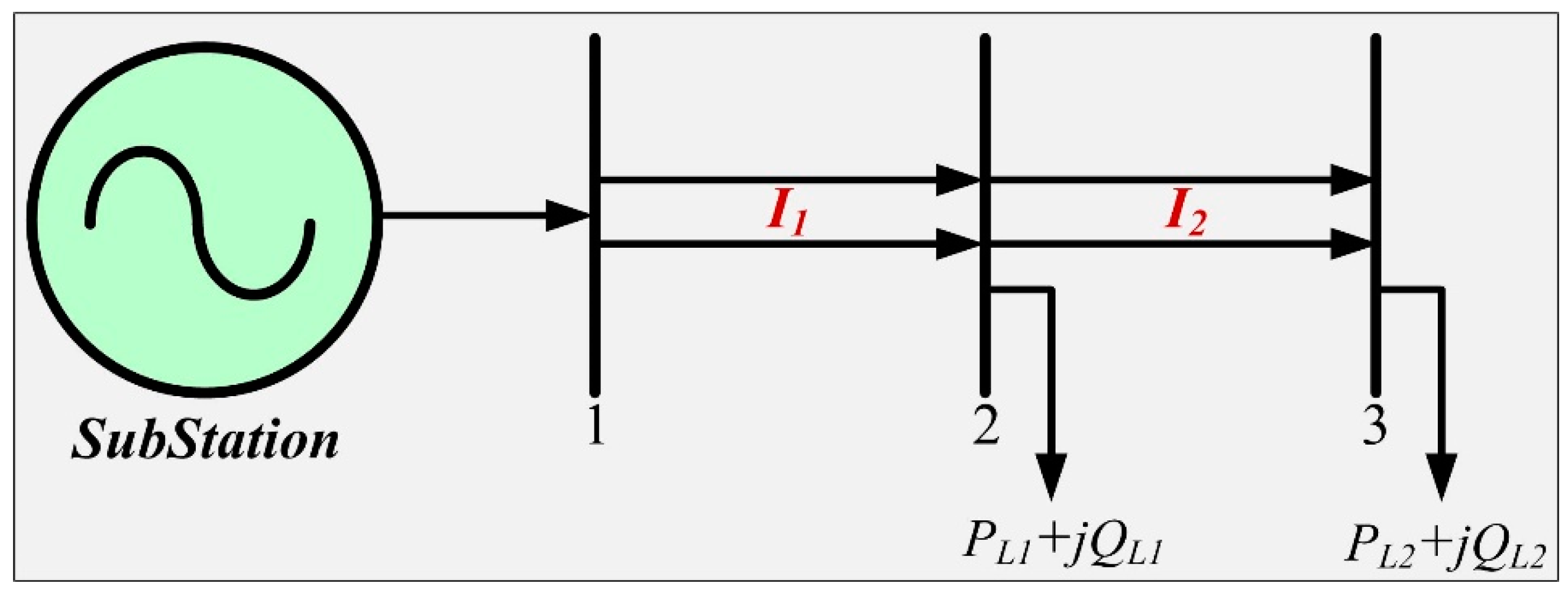
Let us assume an ‘n’ bus test system of radial nature. Figure 2 represents the single line diagram. In this diagram it is assumed that Ii is the current of ith branch. Further, (PLi + jQLi) is the load at ith bus and (Pi + jQi) power flow at the sending end of the ith branch. In these abbreviations, PL denotes the active power component of the load, and QL denotes the reactive power component of the load power.

Figure 2.
Single line diagram for n-bus test radial distribution network.
Expression for phasor current in ith branch has been expressed as
where, is the conjugate of phasor voltage at bus i, as it is assumed that the voltage magnitude at different buses remains closed to 1.0 p.u. after DG integration, therefore the magnitude of current Ii in ith branch can be approximated as
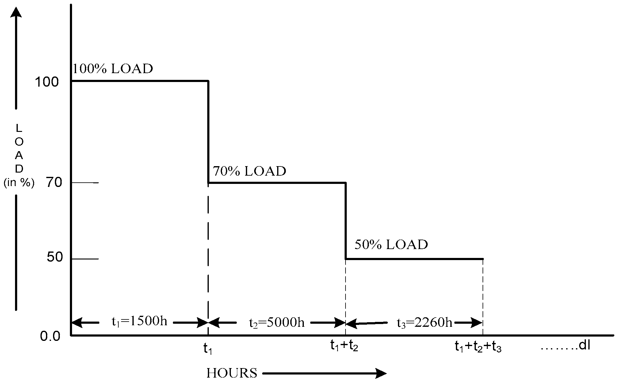
In the present paper, three different load levels (50%, 70% and 100%) with reference to system peak load have been considered. The yearly load duration curve is depicted in Figure 3. The current in various branches is computed by load flow analysis for each load level. Therefore, the magnitude of Ii as given by (2) is calculated as:
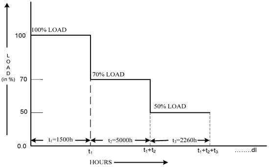
Figure 3.
Load duration curve for different load levels.
The total energy loss for different load levels and durations is calculated in an equation and its description is given as follows:
Here, n is the number of nodes of the system, EL is the system energy loss, Ri is the resistance of the ith branch of the system, dl denotes the number of various levels of load, ts represents the corresponding duration of the ‘sth’ load levels and is the current in the ith branch during the sth load level. The value of EL has been calculated on the basis of (5) using the value of from (3)
Here, & is the injected active and reactive component of power at ith bus for sth load level.
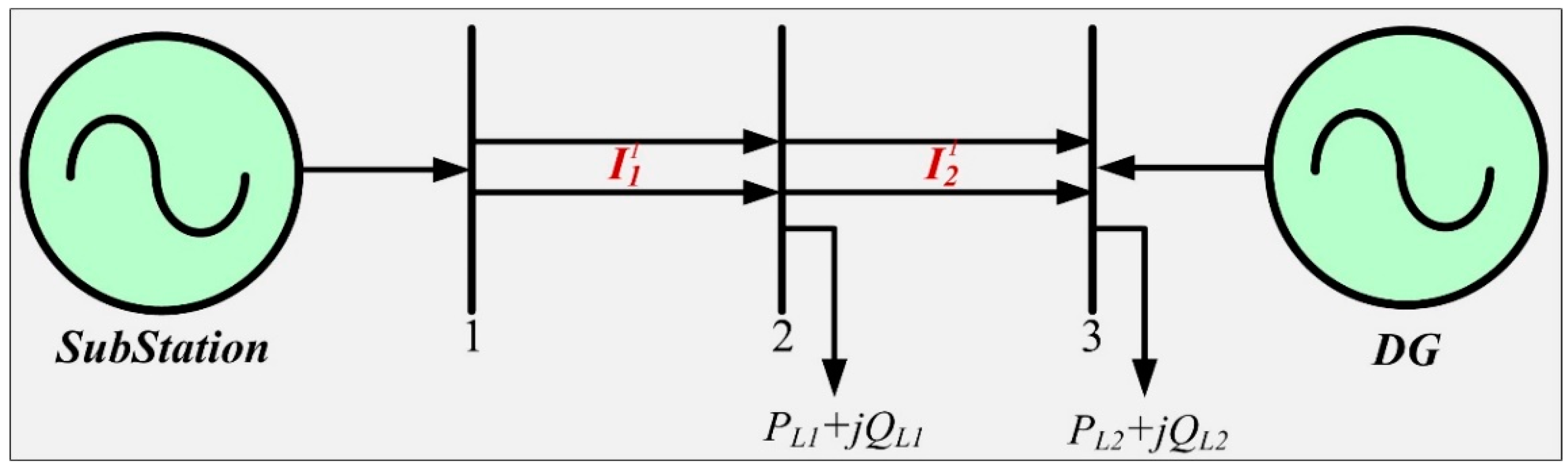
Now, suppose a DG unit is sited at the kth bus of the considered system as depicted in Figure 4; because of the placement of DG units at the kth bus, the current changes in those branches which are in between bus 1 and bus k. While the current magnitude in the leftover branches remains the same.
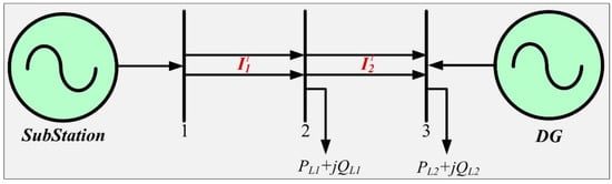
Figure 4.
Single line diagram for n-bus test radial distribution network with DG.
The represents the magnitude of phasor current in ith branch after DG integration and represent the active component and reactive components of injected power at ith bus after DG placement. The expression for after DG placement is given by (6)
where Idg is the phasor current injected by DG unit and Di is the matrix which contains binary values given as
The phasor current supplied by DG can be given as
Here Pdg and Qdg are the components of active and reactive power injected from DG, or basically, it is the optimal capacity of the DG unit. In the present methodology it is assumed that the voltage magnitude at different buses is close to 1.0 p.u., therefore the current injected by the DG unit, i.e., Idg, can be approximated as (8)
Using (6) and (8) is expressed in Equation (9) whose description is given below:
2.2. System Energy Loss Due to the Placement of a Single DG Unit
Due to the allocation of DG in the distribution system the current in network branches is changed; therefore, the system losses are also changed. Hence system energy losses after DG placement can be given as:
where ELN is system energy loss after the placement of DG.
Substituting the values of from (9), the Equation (10) reduces to
Here & are the real and reactive powers of the ith branch for different load levels. Using (5) and (11) for energy loss savings of the system after DG placement
For maximum energy loss saving, partial differentiation of Equation (12) with respects to Pdg and Qdg should be zero as
Solving (13) and (14) for Pdg and Qdg, respectively
The final optimum size of DG will be as
Sdg = Pdg + jQdg
And the optimum power factor of the DG unit is given as
2.3. Formulation for System Energy Loss by Placement of Multiple DG Units
The present section is similar to the previous section, which is developed for the single DG placement of the present study. For the installation of multiple DG units, m is the number of DG units to be placed in an n-bus distribution network. The placement of DGs at various nodes changes the magnitude of the current in system branches; hence, the new current in the ith branch is expressed as ; where is the phasor current injected from jth DG. Further, Dij is given as
The phasor current supplied by jth DG is similar to (7). By considering different load levels, the energy losses after placement of m DGs in the system can be given as
where ELnew is the energy losses in the system after installation of m DG units in the system, using (5) and (19) the net energy loss saving after multiple DG placements can be given as:
Maximum loss saving of energy of system is obtained with installation of multiple DGs by taking the partial derivative of SEN with respect to & , j = 1 to m and equating to zero as
Differentiating (20), partially w.r.t & and equating as zero are represented as follows
Equation (21) provides a set of 2m linear equations, out of which m are as (22) and rest equations are as (23). These 2m equations can be expressed in the form of a matrix as:
[Pdg] and [Qdg] are vectors, which represent the active and reactive power components injected from DG. A is a matrix of size . B and C are the column vectors containing m elements. The elements of matrices A, B and C can be determined as
where Axy represents (x, y)th element of matrix A. Bx and Cx are the xth element of matrix B and C respectively. Further, [Pdg] and [Qdg] can be expressed as
By solving (26) and (27), the optimum size and power factor of jth DG can be calculated as
where Equation (32) is the optimal power factor of DG unit.
The different equations from (1) to (32) are derived by the proposed technique. The base of these derivations is energy loss savings (subtraction of system energy loss with DG from system energy loss without DG). Differentiating Equation (12) partially with respect to Pdg and Qdg, respectively, and equate the equation so obtained in order to obtain the optimum capacity of DG by proposed analytical technique for single DG. Differentiating Equation (20) partially with respect to Pdg and Qdg, respectively, and equate the equation so obtained in order to obtain the optimum capacity of DG by the proposed analytical technique for multiple DG. All these equations so obtained are described in different equations from Equations (13) and (14) for single DG and (22) and (23) for multiple DG.
3. Algorithm for Solution
The formulations which are described in Section 2.1 and Section 2.2 are applied to find the expressions for the optimal size of DG unit. Further, the proposed method is tested on IEEE 69-bus and 33-bus test radial distribution networks, respectively. In the proposed method ‘m’ numbers of DG units are to be placed in an n-bus network. Therefore, there are ncm probable combinations for different buses. These possible combinations become very large in the case of m << n, hence computationally it is very difficult to analyze all combinations [3]. Therefore, the following steps are taken to compute the optimum sizing and bus where DG is to be placed for the purpose of the reduction of the loss of system energy in the test radial distribution network. The flow chart of the proposed algorithm is depicted in Figure 5. The required data is taken from [24].
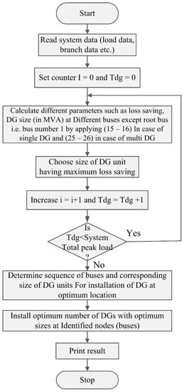
Figure 5.
Flowchart for the placement of multiple DG in the radial distribution system.
- Step 1:
- Read corresponding system data such as (line data, load data, load levels and duration) and run load flow program for base case using BFS-based method, and evaluate the active and reactive component of the powers and current in different branches along with sending end voltage.
- Step 2:
- Set counter at i = 0 for bus number and Tdg = 0 for DG size.
- Step 3:
- Determine DG size and corresponding loss savings by using (17) and (12), respectively, at each bus except the root bus.
- Step 4:
- Increase DG counter, i = i + 1; and DG size Tdg = Tdg + |Sdg|.
- Step 5:
- Check Tdg ≤ Total peak load of the system. If yes, go to step 3; otherwise, go to step 7.
- Step 6:
- Categorize the node number and corresponding DG size where maximum loss saving occurs; this bus number serves as a candidate bus for DG placement.
- Step 7:
- Install DG unit of size obtained from step 6 at the candidate bus which is obtained from step 6 and continue the process till negative or zero loss saving, and thus obtain the sequence of candidate buses
- Step 8:
- For multi-DG placement, use the sequence of buses which is obtained from step 7, and install DG units of the size calculated by (31) and (19) and perform load flow analysis to determine system energy loss and voltage profile.
4. Results and Discussion
In this section IEEE 69-bus and 33-bus radial, networks are considered for testing the developed technique. The method under consideration has been implemented in MATLAB environment to determine the optimum allocation and sizing of DGs. In proposed method the DG units which are capable to inject active and reactive both are considered for placement in the distribution system.
In the proposed method, the sequence of candidate bus for DG placement is identified on the basis of the power loss saving criterion. Further, the bus which has highest power loss saving is considered for DG placement and this process will continue till zero or nearly zero power loss saving is obtained. Therefore, in figures number 7 to 11, the power loss saving has appeared.
The details of simulation results are presented in Table A2, Table A3 and Table A4. These tables are given in Appendix A at the end of this manuscript.
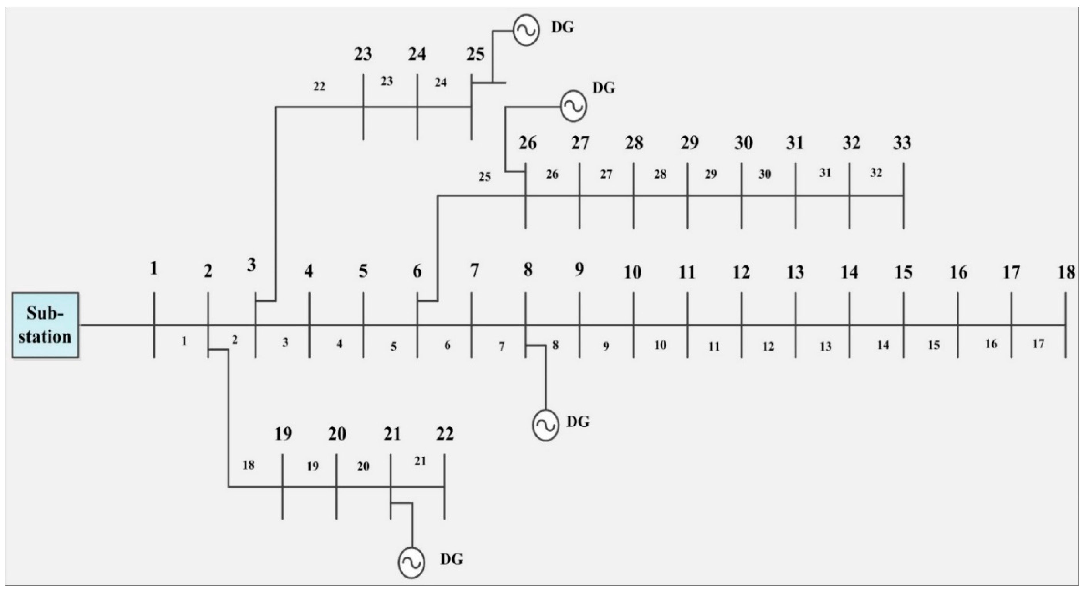
4.1. IEEE 69-Bus Test Radial Distribution System
The Figure 6 is used for the representation of a single-line diagram of the IEEE 69-bus test radial distribution network. This system has a total peak load of (3.80219 + j2.69460) MVA. This given yearly load of the system is divided into three levels. Furthermore, active and reactive components of energy loss due to the branch current are obtained as 93.22 MWh, and 41.86 MVARh, respectively, for the base case, i.e., without DG from load flow solutions.
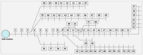
Figure 6.
Single line diagram for IEEE 69-bus test radial distribution system.
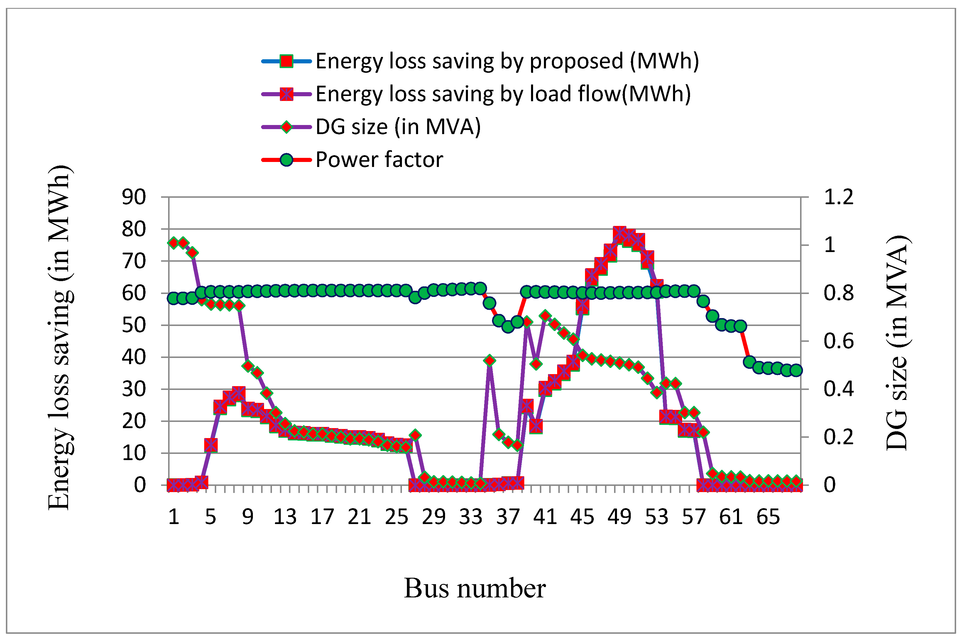
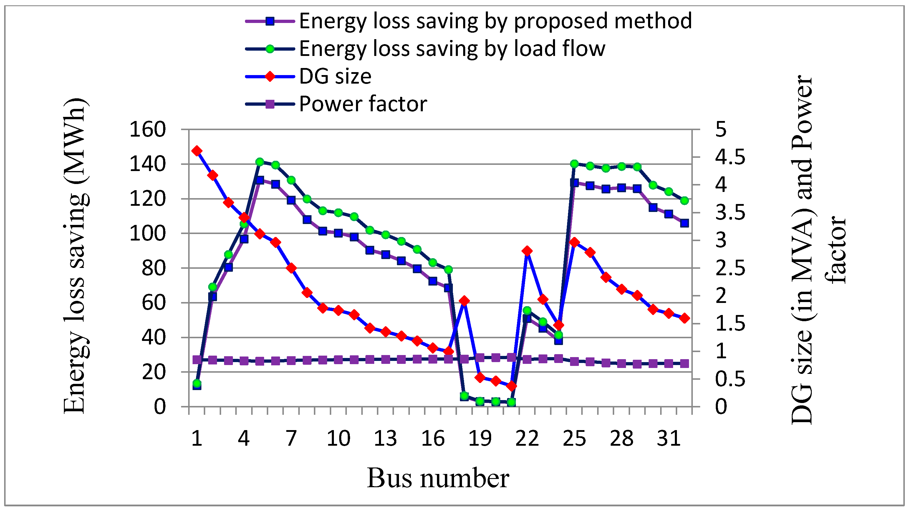
Initially, optimum sizing of DGs and corresponding saving of energy loss at different buses has been determined by (17) and (12), respectively. Further, Figure 7 shows the active energy loss savings followed by optimum size of DGs (in MVA) and along with power factors of these DGs at various nodes for IEEE 69-bus network. Moreover, as is evident from Figure 7, the maximum saving of energy loss is 77.1758 MWh which occurs at node 50, and the corresponding DG size is of (0.4093 + j0.3041) MVA at the same bus number 50.
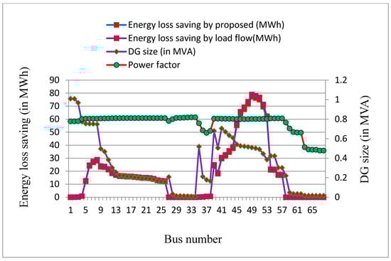
Figure 7.
Optimum DG size (in MVA) and active energy loss saving (in MWh) by proposed method and load flow method at the different bus for 69-bus radial distribution system.
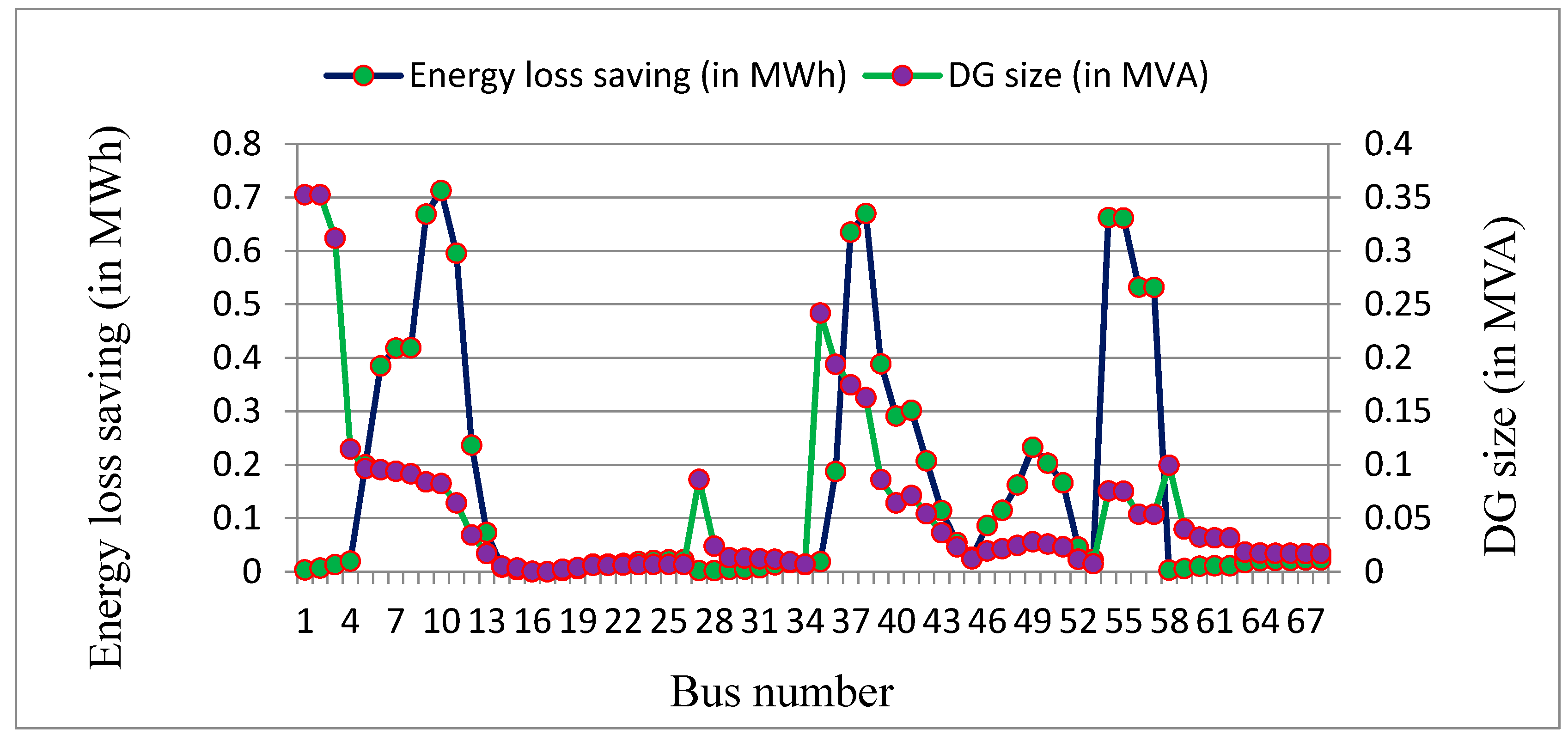
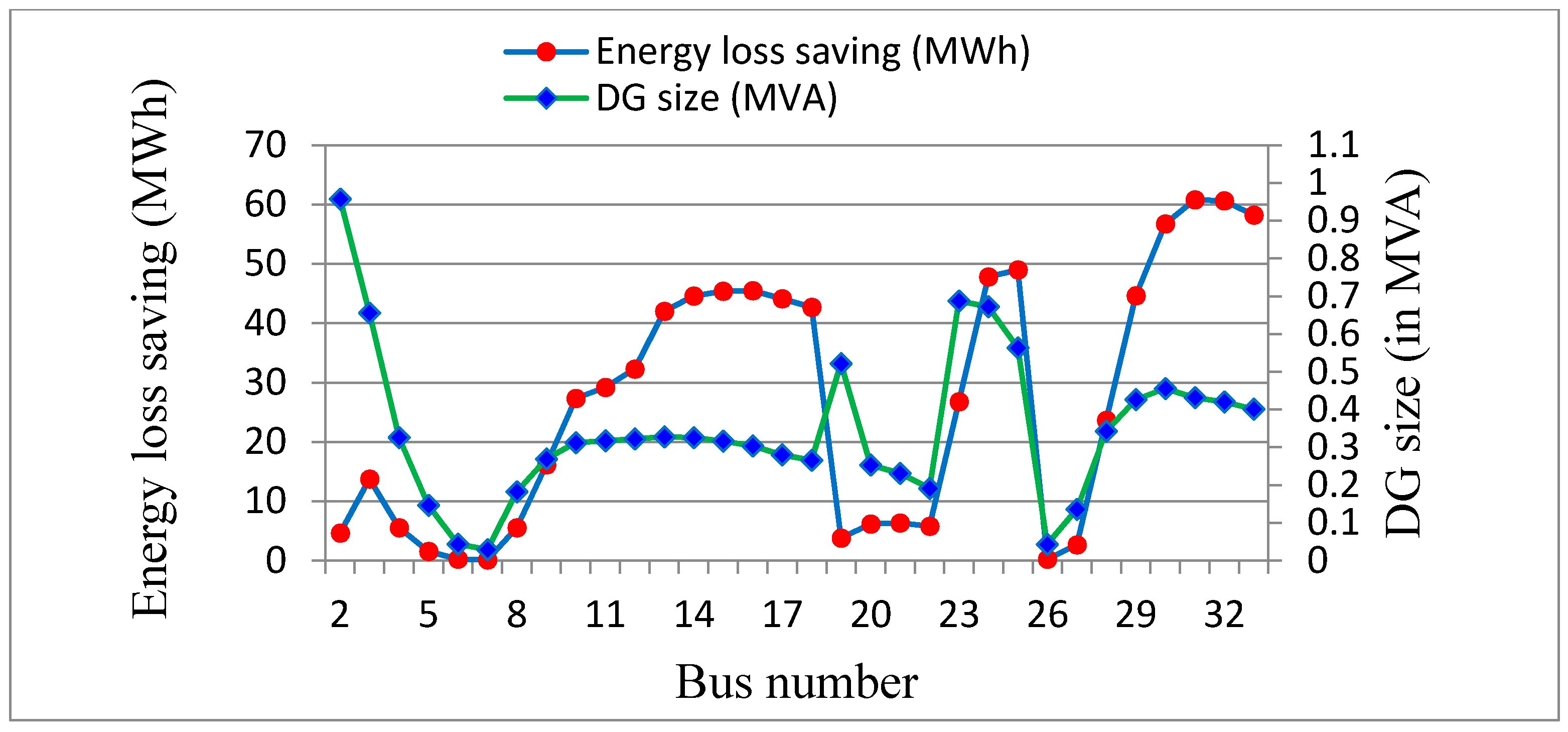
Therefore, install a DG unit of size (0.4093 + j0.3041) MVA at bus number 50 and run the load flow program in order to obtain the next bus for DG placement. In this process a maximum energy loss saving of 6.644186 MWh is observed at bus number 17 and its corresponding DG size (0.1128 + j0.0804) MVA at bus number 17 as it is shown in Figure 8. Therefore, bus number 17 serves as the candidate bus for the second DG unit placement. In this process, the 84.70% of real power loss reduction is observed. To search other buses for DG placement, this process will remain to continue till zero power loss saving is achieved. In these series two buses, 50 and 17, are identified for DG installation.
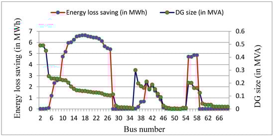
Figure 8.
Loss savings of active energy component with subsequent size of DGs (in MVA) for different nodes for first iteration with DG placed at node 50 for IEEE 69-bus system.
Moreover, DGs of size (0.4093 + j0.3041) MVA and (0.1128 + j0.0804) MVA are placed at bus number 50 and 17, and results are depicted in Figure 9. From Table A2, the energy loss saving of 6.62 MWh is observed after placing a DG of the above-mentioned size at bus numbers 50 and 17. Further, bus number 11 is observed as the candidate bus whose size is (0.066318 + j0.048861) MVA. In this process the method reduces the system power loss by 91.84% as is evident from Table A2. The total size of the DG units is (0.6221 + j0.3845) MVA, which is less than that of system peak load. Additionally, the proposed method keeps on continuing to find the DG size and candidate bus for a third DG unit. Now three DG units of sizes (0.4093 + j0.3041) MVA, (0.1128 + j0.0804) MVA and (0.066318 + j0.048861) MVA obtained from the above process are placed at buses 50, 17 and 11, respectively. It is observed from Figure 10 that maximum energy loss savings occurs at bus 39 with a corresponding DG of size (0.1098 + j0.1195) MVA, the value of the maximum loss savings at bus 39 is 0.666570 MWh. Moreover, in this iteration, the system energy loss is reduced by 92.61%. In the fourth iteration, the total size of DG becomes (0.6326 + j0.5040) MVA which is less than that of the total load on the system. In these iterations the 50, 17, 11 and 39 buses are identified as optimal buses for DG placement and corresponding DG sizes. These buses are (0.4093 + j0.3041) MVA, (0.1128 + j0.0804) MVA, (0.066318 + j0.048861) MVA and (0.1098 + j0.1195) MVA, respectively.
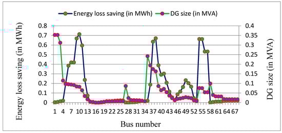
Figure 9.
Loss saving of active energy component with corresponding sizes of DGs (in MVA) at different nodes for the second iteration when DGs are placed at nodes 3 and 6 for IEEE 69-bus system.
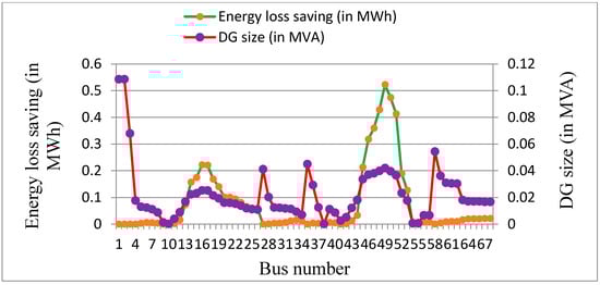
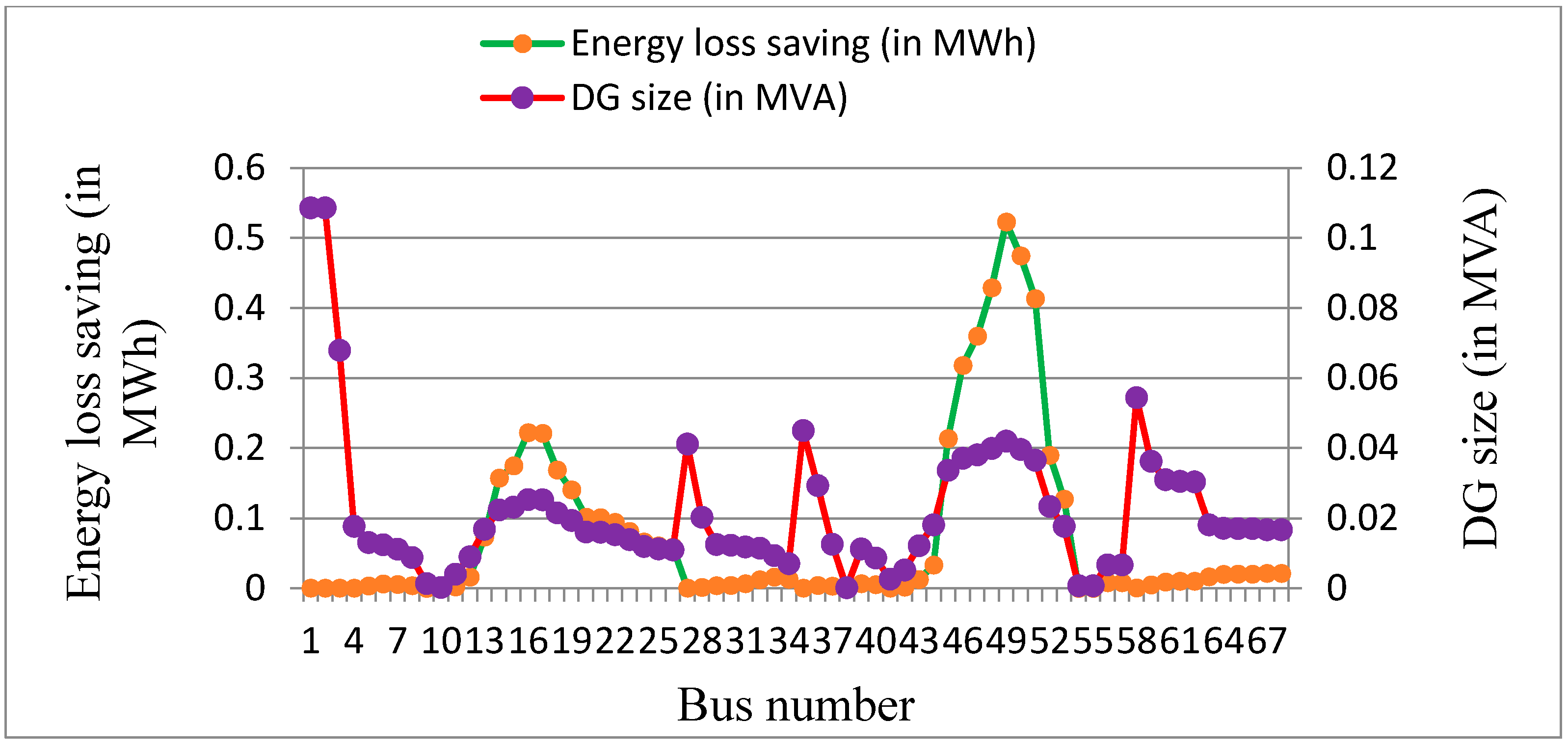
Figure 10.
Loss saving of active energy components with the subsequent size of DGs (in MVA) for different nodes for the third iteration with DGs placed at nodes 50, 17 and 11 for IEEE 69-bus system.
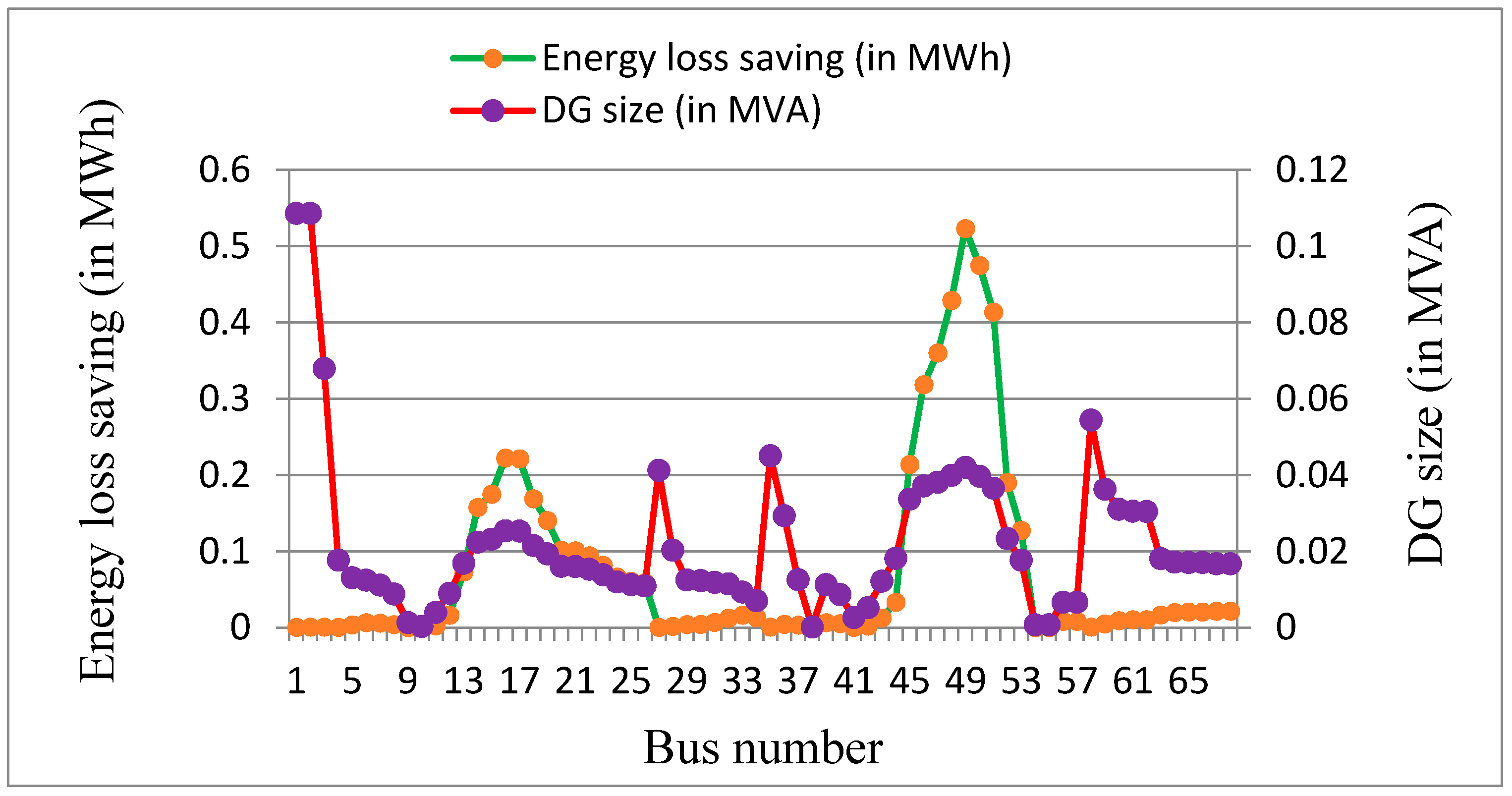
Finally, Figure 11 provides the information that is for four DG units of the size mentioned above, the maximum energy loss saving is on bus 50. Further, it is noticed that the maximum energy loss saving was obtained on node 50 in the first iteration. Therefore, the procedure is converged, and in this whole process, the sequence of buses for DG placement obtained is 50, 17, 11 and 39, and the system energy loss reduces by 93.25%. Finally, the total DG size becomes (0.698232 + j0.552889) MVA, which is less than that total load on the system. The detail of these results is presented in Table A2.
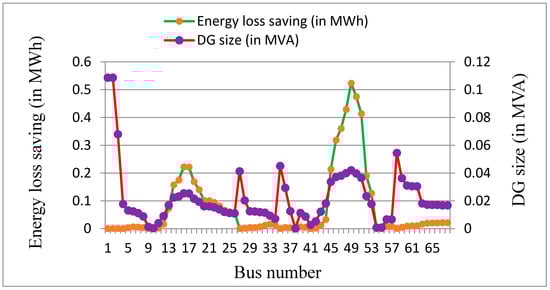
Figure 11.
Loss savings of active energy components with subsequent sizes of DGs (in MVA) for different nodes for the fourth iteration with DG placed at nodes 50, 17, 11 and 39 for IEEE 69-bus system.
Additionally, for siting of multiple units of DG in IEEE 69-bus system size and locations of DGs has been determined by the method which is described in Section 2.3. In this process, the sequence of candidate buses for DG placement is the same as was determined in the preceding section as per this, the sequence of buses is 11, 17, 39 and 50 and the corresponding sizes are (0.115766 + j0.083357) MVA, (0.083643 + j0.059049) MVA, (0.109937 + j0.119590) MVA and (0.375638 + j0.280022) MVA, respectively. The system active component of energy loss without DG and with DG becomes 93.22 MWh and 5.36 MWh, respectively.
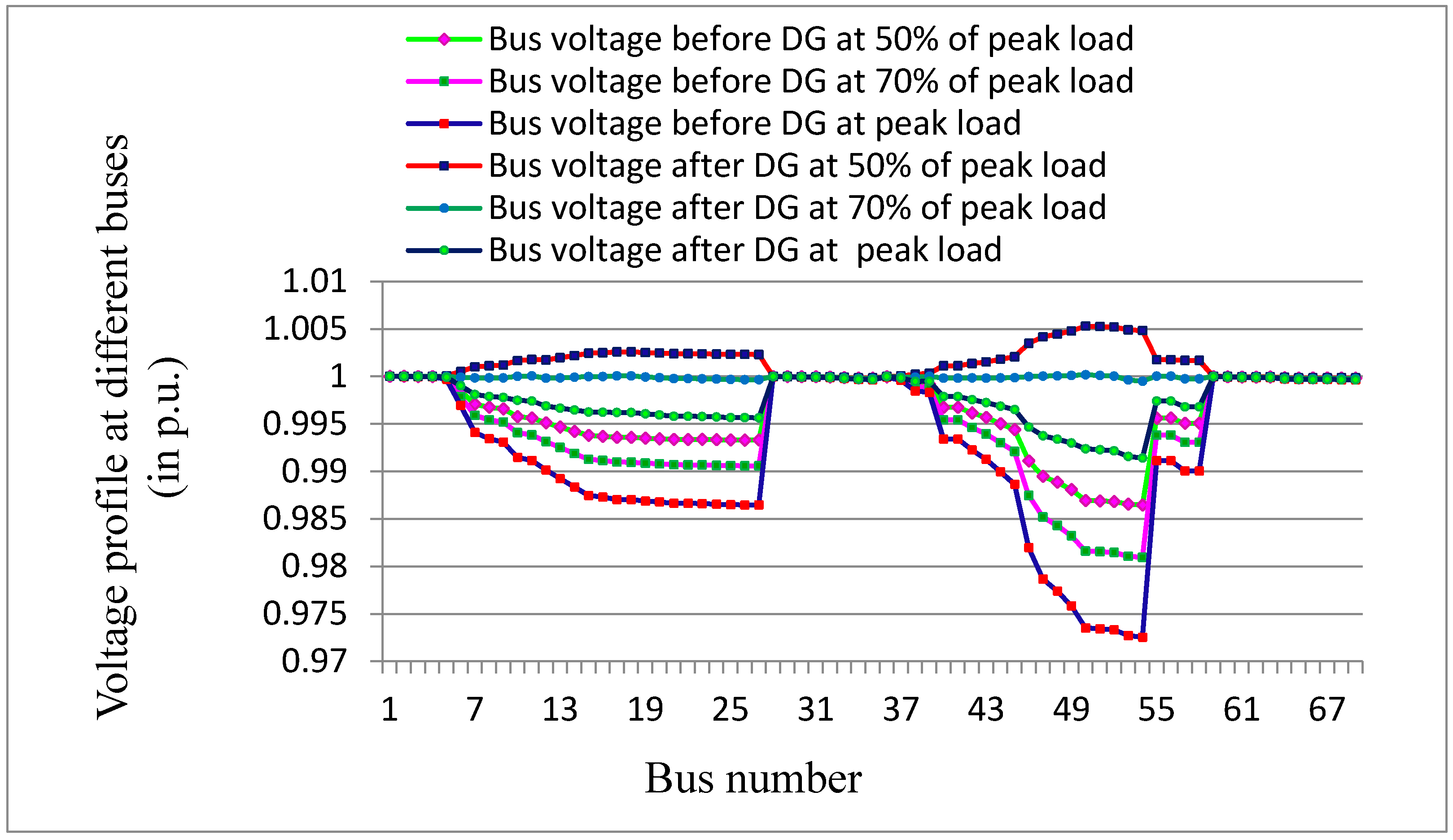
Figure 12 represents the profile of bus voltage for the IEEE 69-bus system with and without DG for various load levels. From this figure it is noticed that the allocation of DG improved system bus voltage significantly. Further, a maximum and minimum value of voltage with and without DG for various load levels ise presented in Table A4.
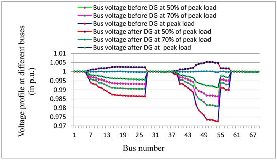
Figure 12.
Voltage profile of IEEE 69-bus radial distribution network at different load levels before and after placement of DG unit.
4.2. IEEE 33-Bus Test Distribution Network
Figure 13 shows the single line diagram of 12.66 kV, 1 MVA IEEE 33-bus radial distribution network having a load of (3.715 + j2.300) MVA. System total energy losses in the form of real and reactive components without DG are 884.95 MWh and 589.77 MVARh, respectively.
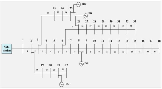
Figure 13.
IEEE 33-bus test distribution system.
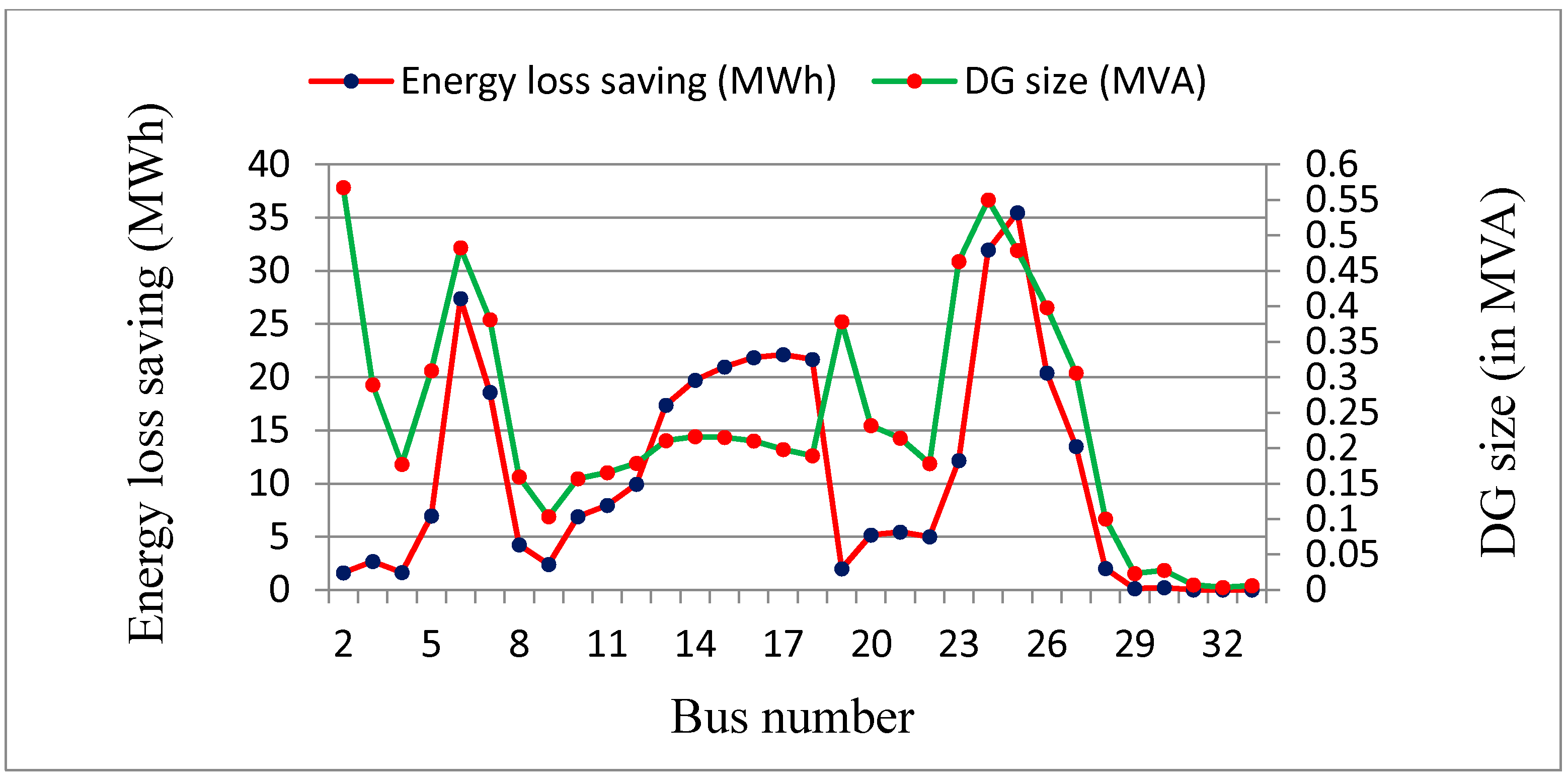
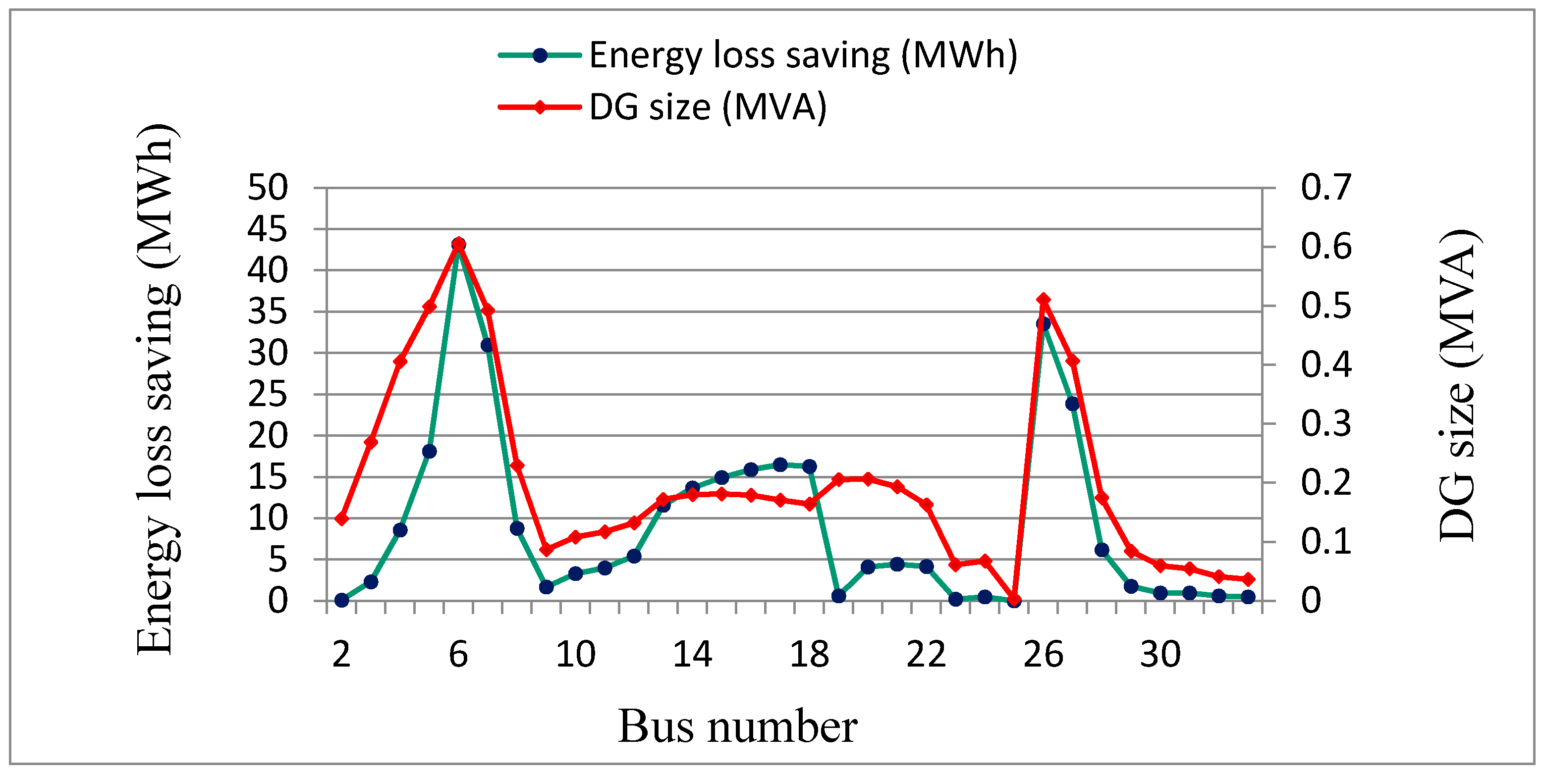
Firstly, the optimum sizes of individual DG units and the corresponding energy loss savings of these DG units have been calculated by developed formulation using Equations (17) and (12). Figure 13 represents the optimum power factor and size of the DG units (in MVA) and the consequent active loss saving (in kW) at various nodes for the IEEE 33-bus system. From Figure 14 the maximum active power loss saving (130.71 kW) occurs at bus 6, and the corresponding DG size (1.772 + j1.220) MVA at the same bus. Therefore, bus 6 serves as a candidate bus for DG placement. Placing a DG unit of size (1.772 + j1.220) MVA at bus 6 provides a maximum loss savings of 60.78 kW at node 31 shown in Figure 15, and the next optimum size of DG unit is (0.295 + j0.314) MVA at node 31. In this process system, energy loss is reduced by 66.22%. In second iteration, bus 31 becomes a candidate node for DG installation. Further, a second DG unit of (0.295 + j0.314) MVA is installed at node 31 gives rise to the maximum energy loss of 35.48 MWh along with DG unit of (0.445 + j178) MVA at bus 25 as it is depicted in Figure 16. Moreover, the system loss reduces by 73.21%.
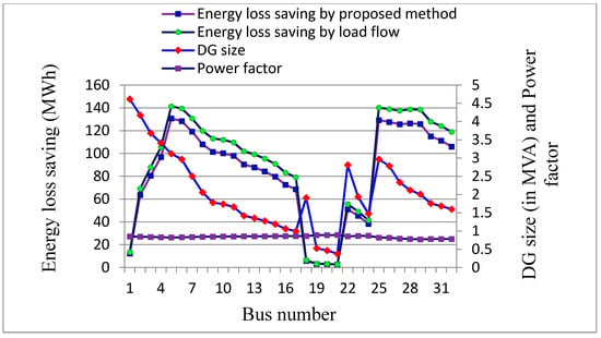
Figure 14.
DG units’ size (in MVA), power factor and energy loss saving (in MWh) at various nodes for the IEEE 33-bus radial distribution system.
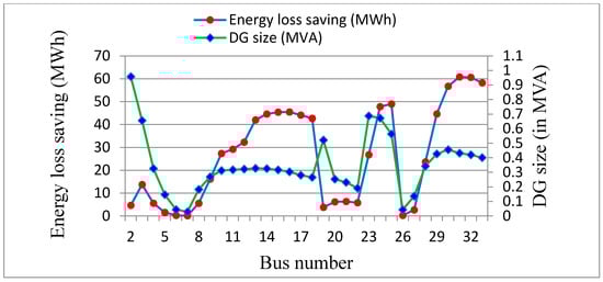
Figure 15.
Optimal DG size (in MVA) and corresponding energy loss saving (in MWh) with DG at node 6 for various nodes for the IEEE 33-bus system.
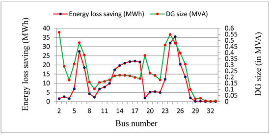
Figure 16.
DG sizes (in MVA) with DG placed at nodes 6 and 31 and corresponding energy loss saving (in MWh).
Furthermore, a third DG unit of (0.445 + j178) MVA installed at node 25 gives a maximum loss savings of 26.14 kW further at node 6 along with a DG of (−0.460 − j0.394) MVA at the same node as is shown in Figure 17. Further, it is observed that first –ve sized DG is on bus 6, which is identical to the bus which was obtained in the very first iteration. Further, it is important to mention that initially the DG at bus 6 was oversized. Further, to obtain the optimal size of DG unit at bus 6 by subtracting (−0.460 − j0.394) MVA from the initially obtained size, i.e., (1.772 + j1.220) MVA, therefore, the optimum size of DG unit at bus 6 is (1.312 + j0.826) MVA. Thus, the identified sequence of candidate buses for DG placement is 6, 31 and 25. In this process, the system loss is reduced by 82.12%.
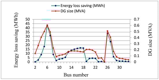
Figure 17.
DG sizes (in MVA) and energy loss saving (in MWh) with DG units are placed at nodes 6, 31 and 25 for IEEE 33-bus system.
The method described under sub-section C of section II of this study has been applied for the installation of multiple DGs in IEEE 33-bus network. Equations (19) and (28) have been applied to determine the net energy loss savings and optimum sizes of DG units, respectively. Further, DG units having sizes of (1.141 + j0.643) MVA, (0.482 + j0.505) MVA and (0.551 + j0.267) MVA are placed at the identified buses 6, 31 and 25, respectively, provide system energy loss reduction from 884.95 MWh to 144.38 MWh with 83.69%. Moreover, the placement of the above-mentioned sizes of DGs at the respective places, i.e., the 6, 31 and 25 number buses, gives rise to energy loss savings of 740.57 MWh.
In this entire process, the system energy losses get reduced from 884.95 MWh to 298.98 MWh with 66.22% in case of the methodology of single DG placement. Further, in case of the multiple DG placement methodology, three DG units are placed at identified buses, these are 6, 31 and 25 of sizes mentioned above, the active energy losses of the system reduced from 884.95 MWh to 144.38 MWh with 83.69%.
The detailed results of IEEE 33-bus system with respect to DG sizes, energy loss saving and percentage of energy loss reduction have been presented in Table A3.
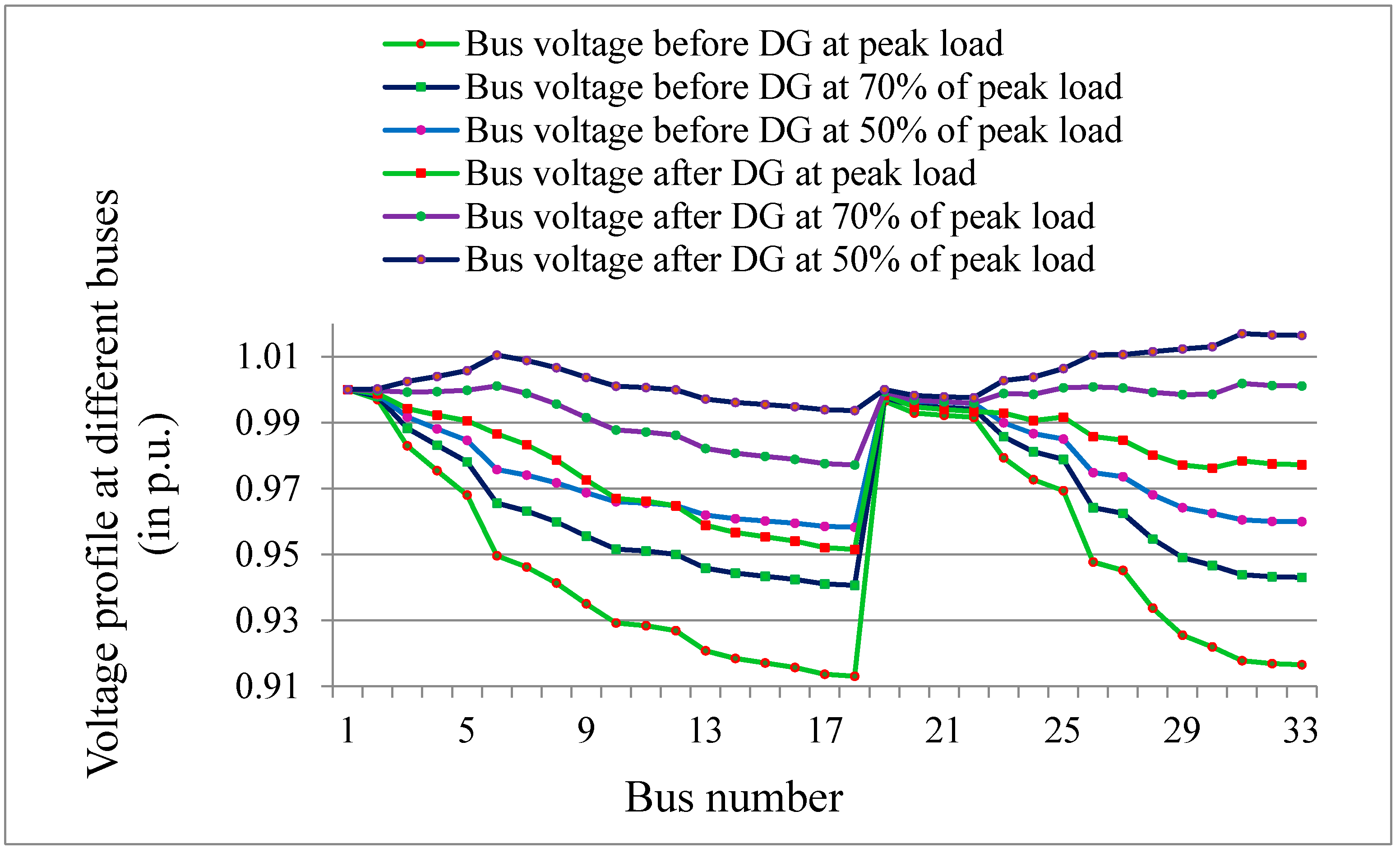
Figure 18 shows the profile of system voltage of IEEE 33-bus system without and with DG unit installation for three load levels it is noticed from this figure that voltage profile of system enhanced significantly. On the basis of these results it is concluded that branch current is reduced due to the installation of DG in the network, and as a consequence, the system voltage profile gets improved. Further, the maximum and minimum values of bus voltage without and with DG for the three load levels is presented in Table A4. From this table it is noticed that the minimum voltage (0.9582 p.u.) appears at bus 18 in the base case, i.e., without DG placement, and this value of voltage is increased up to 0.9936 p.u. for 50% load, and the same pattern is observed for other load profilis, i.e., 75% and 100% load. Table A5 represents the comparison of different results obtained by the proposed method and the results achieved by other methods which are available in the literature. On the basis of obtained results, it is found that the power loss saving capability is more as compared to other methods in the case of a 33-bus radial distribution system. Size of DG is also less as compared to other methods. It is also observed from Table A5 that the optimal locations of DGs by the proposed method are also similar to other available methods for 33-bus and 69-bus test radial distribution systems. Therefore, this phenomenon proves the suitability of this proposed method. Further, Table A6 represents the description of data with respect to different load levels and durations which is considered in the proposed method.
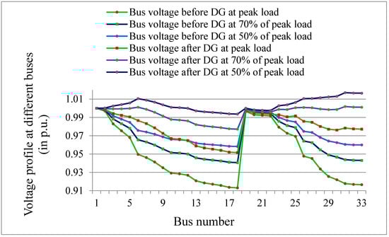
Figure 18.
Bus voltage for IEEE 33-bus system for various load levels before and after DG placement at different bus.
5. Conclusions
The objective of the present research article is to decrease system energy loss with optimum sizing and placement of DG by applying an analytically based method. There is no need oof the formation and computation of the admittance matrix in the developed method. The present technique is intended to identify the order of buses to DG installation by process of maximum energy loss saving of real components of energy. The developed method is valid for multiple DGs along with single DG in test radial distribution systems. Moreover, this developed method is more advantageous over the other method because it requires only a few power flow solutions in order to find out the optimum DG size even for larger networks. The developed modus operandi is applied on an IEEE 69-bus and 33-bus network. The simulation results obtained by the present developed approach are compared with the other methods which are discussed in literature, and it is established that the energy loss reduction capability of the proposed method is more as compared to other methods. The basic and foremost objective of present study is to minimize energy loss and to obtain the optimum position of DG placement and hence, improvement in voltage profile.
Author Contributions
Conceptualization, H.M.; Data curation, P.P., D.C.M., H.M. and I.A.K.; Formal analysis, P.P., D.C.M., H.M., M.A.A. and I.A.K.; Funding acquisition, P.P., H.M., M.A.A. and I.A.K.; Investigation, P.P. and H.M.; Methodology, P.P., D.C.M., H.M., M.A.A. and I.A.K.; Project administration, D.C.M., H.M. and M.A.A.; Resources, P.P., H.M., M.A.A. and I.A.K.; Software, P.P. and D.C.M.; Supervision, D.C.M. and I.A.K.; Visualization, P.P., D.C.M. and M.A.A.; Writing—original draft, P.P., H.M., M.A.A. and I.A.K.; Writing—review & editing, M.A.A. All authors have read and agreed to the published version of the manuscript.
Funding
The authors extend their appreciation to the Researchers Supporting Project at King Saud University, Riyadh, Saudi Arabia, for funding this research work through the project number RSP-2021/278.
Institutional Review Board Statement
Not applicable.
Informed Consent Statement
Not applicable.
Data Availability Statement
Not applicable.
Acknowledgments
The authors would like to acknowledge the support from King Saud University, Saudi Arabia. The authors would like to acknowledge the support from Intelligent Prognostic Private Limited Delhi, India Researcher’s Supporting Project.
Conflicts of Interest
The authors declare no conflict of interest.
Appendix A
The following procedure is adopted for the formation of a D matrix for multiple DG allocation. Suppose four DG units are to be installed at buses 8, 21, 25 and 26 in an IEEE 33-bus system. Here m is total number of DG units which are to be placed. Therefore, m = 4 and the set of branches βj containing the branches between bus j where DG is to be installed, and source bus is given as
- m = 4,
- β8 = {1, 2, 3, 4, 5, 6, 7}
- β21 = {1, 18, 19, 20}
- β25 = {1, 2, 22, 23, 24}
- β26 = {1, 2, 3, 4, 5, 25}
Let DG is placed at bus no. 8 (β8), due to this magnitude of current is changed in the branches 1, 2, 3, 4, 5, 6, 7 only and current in other branches remains same. DG is placed at bus no. 21 (β21), due to this magnitude of current is changed in the branches 1, 18, 19, 20 only and current in other branches remains same. DG is placed at bus no. 25 (β25), due to this magnitude of current is changed in the branches 1, 2, 22, 23, 24 only and current in other branches remains same. DG is placed at bus no. 26 (β26), due to this magnitude of current is changed in the branches 1, 2, 3, 4, 5, 25 only and current in other branches remains same.
The matrix DT has an order of , where m is 4 that is DG units’ number which are is to be placed, and n − 1 is 32 that is a number of branches that is a column vector of DT matrix. Therefore, the elements of the first row oof the DT matrix will be 1 at columns (1, 2, 3, 4, 5, 6, 7) and the remaining elements in same row are 0. Similarly, the elements of the second row will be 1 at columns (1, 18, 19, 20), and elements of other columns in the same row are 0. The elements of the third row will be 1 at columns (1, 2, 22, 23, 24) and the elements of the other columns are 0 in third row. Finally, the elements of the fourth row will be 1 at columns (1, 2, 3, 4, 5, 25), and elements of the other columns are 0 in the fourth row.
The rows of the above matrix represent buses of the network while columns of the matrix represent branches of the matrix respectively. In the present case, DT is of order ( or ) matrix in same way Dij can be determined for n number of DG.

Table A1.
Summary of the related work.
Table A1.
Summary of the related work.
| Reference Number and Year of Publication | Type of Application | Main Contribution and Characteristics | Analyzed Method/Remarks | Recommended System/Similarity with Current Approach |
|---|---|---|---|---|
| [1], 2001, [13], 2016, [24],1995 | Investigated the impact of penetration level of DG in distribution network | Addressed the transient stability and static performance of large system by considering penetration of DG | Addressed different issues and challenges related to DG placement in distribution system | No similarity |
| [2], 2006, [3], 2014, [4], 2015, [5], 2014, [6], 2004, [7], 2009, [8], 2013, [9], 2013, [10], 2010, [17], 2014, [21], 2016 | All these research paper applied an Analytical method for optimal sizing and siting of DG in distribution system | Investigation of optimal sizing and siting of DG on the basis of loss sensitivity factor and equivalent current injection based analytical methods. The objective functions are optimized by PSO and ELF-absed Technique. In some references the sensitivity of loss factor is applied to minimize the search space. | Authors described an analytical based method for optimum size and location of DG to minimize the total power loss of the system without using Jacobian matrix. The proposed methods are implemented on IEEE 33-bus and 69-bus radial distribution system | Analytical based is addressed which is not using admittance or Jacobian matrix. But in the current method, the analytical-based method is described by using load flow method solutions |
| [11], 2013 | Evolutionary based technique for optimal placement of (wind and solar) based DG in distribution network | Sensitivity indexed based Evolutionary optimization technique is used to optimal placement and sizing of non-dispatchable DG | The proposed technique is applied on IEEE 69-bus distribution network and sensitivity indexed is considered to limit the search space | No similarity |
| [12], 2014 | New multi-objective index (IMO) based method for integration of SPV | An analytical based expressions are derived to for optimal sizing of SPV based | Authors investigate an analytical based method for optimal integration of SPV based DG along with BES (battery energy storage system). The proposed method is applied on IEEE 33-bus distribution system | No similarity |
| [14], 2013 | PSO based optimization technique | Authors investigate the PSO based optimization technique for optimal sizing and siting of different types of DGs in distribution system | The objective of proposed method is to minimize the system power loss by considering placement of different types of DGs. The methodology is tested on IEEE 33-bus and 69-bus radial distribution system | No similarity |
| [15], 2015 | Novel power loss sensitivity and power stability index (PSI) based method | Authors describe comparison of Novel Power Loss Sensitivity, Power Stability Index (PSI), further voltage stability index (VSI) methods for optimal location and sizing of DG in radial distribution network. | The optimal location and sizing of DG is performed by considering load growth. The proposed technique is tested on IEEE 12-bus, modified 12-bus, 69-bus and 85-bus test systems. | No similarity |
| [16], 2013 | Comparison of different novel techniques for optimal sizing and siting of DG | Authors investigate the comparison of different techniques like combined power loss sensitivity, index vector, voltage sensitivity index and modified novel method for optimal sizing and siting of DG | The objective of proposed method to improve system voltage profile and minimize system power loss. The proposed method is applied on IEEE 33-bus and 69-bus radial distribution system | No similarity |
| [18], 2014 | Identification of vulnerable buses for DG placement by bifurcation based method | Placement of optimal number DGs in order maintain system voltage within permissible limit by bifurcation method | The global optimization of optimal number of DGs is found on the basis of dynamic programming search method. The proposed method is applied on 34-bus distribution network | No similarity |
| [19], 2013 | Multi-objective based nonlinear programming (NLP) based method | Optimum sizing and siting of DG in distribution system is performed by NLP based method. The objective of proposed method to improve voltage stability | A fuzzy logic based method by selecting appropriate weight factors is applied to obtain the desired objectives | No similarity |
| [20], 2006 | Application of GA based optimization technique | Authors applied GA technique for optimum sizing and siting of DG to enhance system reliability, system voltage and minimize system losses | The proposed method is demonstrated on standard IEEE test radial distribution network | No similarity |
| [22], 2012 | Indexed based method for DG placement and results are compared by Golden Section Search (GSS) | Authors proposed a new analytical based index (PSI) algorithm for DG placement and sizing in distribution system | The proposed technique is applied on 12-bus, modified 12-bus and 69-bus distribution networks. | No similarity |
| [23], 2013 | MINLP based technique for optimal sizing and siting of DG | Authors proposed a methodology for improving voltage profile and voltage stability margin | The objective of proposed method is to improve VSM and method is tested on standard IEEE test radial distribution system | No similarity |
| [25], 2011 | AC optimal power flow based method | Authors investigate AC optimal power flow (OPF) for optimal penetration of DG to minimize system loss | Optimal penetration and placement of DG using multi-period AC OPF based method. Proposed method is tested on U.K. based distribution network | No similarity |
| [26], 2013, [28]—2018 | PSO based optimization technique | PSO based optimization technique is applied for optimal placement and sizing of DG in distribution system | The objective of proposed method is to minimize of power loss and maximization of voltage stability. The method is tested on 12-bus, 30-bus, 33-bus, 41-bus and 69-bus test distribution system | No similarity |
| [27], 2018 | Selection and integration of best DG in distribution system | Author addressed the impact of reactive power on voltage stability and penetration level by analytical based method | The various indices are evaluated by modal analysis method. The proposed method is tested on 33-bus and 136-bus distribution network | No similarity |
Table A2.
Summary of the simulation results for IEEE 69-bus radial distribution network.
Table A2.
Summary of the simulation results for IEEE 69-bus radial distribution network.
| S.No. | Network Condition | Real Energy Loss (MWh) | Number of DG | Node(s) for DG Placement | Size of DG (Pdg + jQdg) MVA | Size of DG (in MVA) | Optimum DG Power Factor | Loss Saving (MWh) | Active Energy Loss Reduction in (%) |
|---|---|---|---|---|---|---|---|---|---|
| 1. | Without DG | 93.22 | - | - | - | - | - | - | - |
| 2. | 0.409 + j0.304 MVA, DG placed at bus 50 | 77.18 | 1 | 50 | 0.409 + j0.304 | 0.510 | 0.8025 | 14.55 | 84.39 |
| 3. | 0.409 + j0.304 MVA DG placed at bus 50 and 0.113 + j0.080 MVA DG placed at bus 17 | 7.62 | 2 | 50 17 | 0.409 + j0.304 0.113 + j0.080 | 0.139 | 0.8162 | 6.64 | 91.84 |
| 4. | 0.409 + j0.304 MVA DG placed at bus 50, 0.113 + j0.080 MVA DG placed at bus 17, and 0.066 + j0.048 MVA DG at bus 11 | 6.88 | 3 | 50 17 11 | 0.409 + j0.304 0.113 + j0.0800.066 + j0.048 | 0.082 | 0.8087 | 0.713 | 92.61 |
| 5. | 0.409 + j0.304 MVA DG placed at bus 50, 0.113 + j0.080 MVA DG placed at bus 17, 0.066 + j0.048 MVA DG at bus 11, and 0.110 + j0.120 MVA DG at bus 39 | 6.21 | 4 | 50 17 11 39 | 0.409 + j0.304 0.113 + j0.0800.066 + j0.0480.110 + j0.120 | 0.162 | 0.6757 | 0.667 | 93.32 |
| 6. | Base case | 93.22 | - | - | - | - | - | - | - |
| 7. | 0.116 + j0.083 MVA, DG at bus 11, 0.084 + j0.059 MVA DG at bus 17, 0.110 + j0.120 MVA DG at bus 39 and 0.376 + j0.280 MVA DG at bus 50 | 93.22 | 4 | 11 17 39 50 | 0.116 + j0.083 0.084 + j0.059 0.110 + j0.120 0.376 + j0.280 | 0.1427 0.1024 0.1624 0.4685 | 0.8115 0.8169 0.6768 0.8017 | 5.36 | 94.22 |
Table A3.
Summary of simulation results for IEEE 33-bus network.
Table A3.
Summary of simulation results for IEEE 33-bus network.
| S.No. | Network Condition | Real Energy Loss (MWh) | Number of DG | Node(s) Where DG Is Placed | Size of DG (Pdg + jQdg) MVA | Optimum Power Factor of DG | Loss Saving (in MWh) | Real Energy Loss Reduction in (%) |
|---|---|---|---|---|---|---|---|---|
| 1. | Without DG | 884.95 | - | - | - | - | - | - |
| 2. | 1.772 + j1.220 MVA DG placed at bus 6 | 298.98 | 1 | 6 | 1.772 + j1.220 | 0.8237 | 544.34 | 66.22 |
| 3. | 1.772 +j1.220 MVA DG placed at bus 6 and 0.295 + j0.314 MVA DG placed at bus 31 | 237.11 | 2 | 6 31 | 1.772 + j1.220 0.295 + j0.314 | 0.8237 0.6847 | 60.78 | 73.21 |
| 4. | 1.772 + j1.220 MVA, DG placed at bus 6, 0.295 + j0.314 MVA, DG placed at bus 31, and 0.444 + j0.179 MVA DG placed at bus 25 | 158.27 | 3 | 6 31 25 | 1.772 + j1.220 0.295 + j0.314 0.444 + j0.179 | 0.8237 0.6847 0.9275 | 35.48 | 82.12 |
| Multi-DG (Three-DGs of following size are placed at a time in 6, 25, 31) | ||||||||
| 5. | Base case | 884.95 | - | - | - | - | - | - |
| 6. | 1.141 + j0.643 MVA, 0.8712 PF lag DG at bus 6, 0.482 + j0.505 MVA DG at bus 31 and 0.551 + j0.267 MVA, 0.9 PF lag DG placed at bus 25 | 884.95 | 3 | 6 31 25 | 1.141 + j0.643 0.482 + j0.505 0.551 + j0.267 | 0.8712 0.6903 0.9000 | 144.38 | 83.69 |
Table A4.
Maximum and minimum value of voltage for IEEE 69-bus and IEEE 33-bus network before and after dg placement.
Table A4.
Maximum and minimum value of voltage for IEEE 69-bus and IEEE 33-bus network before and after dg placement.
| System Type | Maximum and Minimum Bus Voltage before DG | Maximum and Minimum Bus Voltage after DG | ||||||||||
|---|---|---|---|---|---|---|---|---|---|---|---|---|
| 50% of Peak Load | 70% of Peak Load | 100% of Peak Load | 50% of Peak Load | 70% of Peak Load | 100% of Peak Load | |||||||
| Minimum Voltage (in p.u.) Bus | Maximum Voltage (in p.u.) Bus | Minimum Voltage (in p.u.) Bus | Maximum Voltage (in p.u.) Bus | Minimum Voltage (in p.u.) Bus | Maximum Voltage (in p.u.) Bus | Minimum Voltage (in p.u.) Bus | Maximum Voltage (in p.u.) Bus | Minimum Voltage (in p.u.) Bus | Maximum Voltage (in p.u.) Bus | Minimum Voltage (in p.u.) Bus | Maximum Voltage (in p.u.) Bus | |
| 69-bus | 0.9864 54 | 1.0000 1 | 0.9809 54 | 1.0000 1 | 0.9725 54 | 1.0000 1 | 0.9998 69 | 1.0053 50 | 0.9995 54 | 1.0002 51 | 0.9914 54 | 1.0000 1 |
| 33-bus | 0.9582 18 | 1.0000 1 | 0.9407 18 | 1.0000 1 | 0.9131 18 | 1.0000 1 | 0.9936 18 | 1.017 31 | 0.9771 18 | 1.0019 31 | 0.9515 18 | 1.0 1 |
Table A5.
Comparison of results by different methods for IEEE 69-bus and 33-bus radial distribution system.
Table A5.
Comparison of results by different methods for IEEE 69-bus and 33-bus radial distribution system.
| System | Parameters | Murty and Kumar [15] | Naik and Khatod [3] | Viral and Khatod [4] | Proposed Technique | ||
|---|---|---|---|---|---|---|---|
| 69-bus | Optimum bus | - | - | 3 | 3 | ||
| DG size | 1.85 MW UPF, 2.20 MVA, 0.9 PF lag | 2.22 MVA, 0.82 PF lag | - | 0.73 MVA, 0.8033 PF lag | |||
| Loss saving (in percentage) | 87.59 at 0.9 PF lag | 89.39 at 0.82 PF lag | - | 94.25 at 0.8033 PF lag | |||
| 33-bus | Optimum bus | 50 | 50 | 50 | 50 | ||
| DG size | 2.5 MVA at UPF | 3.01 MVA 0.9 PF lag | 2.48 MVA UPF | 3.01 MVA at 0.85 PF lag | 2.969 MVA, 0.8180 PF lag | 3.121 MVA, 0.8231PF lag | |
| Loss saving (in percentage) | 47.32 | 66.39 | 48.65 | 69.55 | 33.88 | 83.69 | |
Table A6.
Data for load level and load duration.
Table A6.
Data for load level and load duration.
| Load level (in the percentage of peak load) | 100 | 70 | 50 |
| Time interval (in hours) | 1500 | 5000 | 2260 |
References
- Ackermann, T.; Andersson, G.; Söder, L. Distributed generation: A definition. Electr. Power Syst. Res. 2001, 57, 195–204. [Google Scholar] [CrossRef]
- Acharya, N.; Mahat, P.; Mithulananthan, N. An analytical approach for DG allocation in primary distribution network. Int. J. Electr. Power Energy Syst. 2006, 28, 669–678. [Google Scholar] [CrossRef]
- Naik, S.N.G.; Khatod, D.K.; Sharma, M.P. Analytical approach for optimal siting and sizing of distributed generation in radial distribution networks. IET Gener. Transm. Distrib. 2015, 9, 209–220. [Google Scholar] [CrossRef]
- Viral, R.; Khatod, D. An analytical approach for sizing and siting of DGs in balanced radial distribution networks for loss minimization. Int. J. Electr. Power Energy Syst. 2015, 67, 191–201. [Google Scholar] [CrossRef]
- Kaur, S.; Kumbhar, G.; Sharma, J. A MINLP technique for optimal placement of multiple DG units in distribution systems. Int. J. Electr. Power Energy Syst. 2014, 63, 609–617. [Google Scholar] [CrossRef]
- Wang, C.; Nehrir, M. Analytical approaches for optimal placement of distributed generation sources in power systems. IEEE Trans. Power Syst. 2005, 19, 2068–2076. [Google Scholar] [CrossRef]
- Gözel, T.; Hocaoglu, M.H. An analytical method for the sizing and siting of distributed generators in radial systems. Electr. Power Syst. Res. 2009, 79, 912–918. [Google Scholar] [CrossRef]
- Hung, D.Q.; Mithulananthan, N. Multiple Distributed Generator Placement in Primary Distribution Networks for Loss Reduction. IEEE Trans. Ind. Electron. 2011, 60, 1700–1708. [Google Scholar] [CrossRef]
- Hung, D.Q.; Mithulananthan, N.; Bansal, R. Analytical strategies for renewable distributed generation integration considering energy loss minimization. Appl. Energy 2013, 105, 75–85. [Google Scholar] [CrossRef]
- Hung, D.Q.; Mithulananthan, N.; Bansal, R. Analytical Expressions for DG Allocation in Primary Distribution Networks. IEEE Trans. Energy Convers. 2010, 25, 814–820. [Google Scholar] [CrossRef]
- Khatod, D.K.; Pant, V.; Sharma, J. Evolutionary programming based optimal placement of renewable distributed generators. IEEE Trans. Power Syst. 2012, 28, 683–695. [Google Scholar] [CrossRef]
- Hung, D.Q.; Mithulananthan, N.; Bansal, R. Integration of PV and BES units in commercial distribution systems considering energy loss and voltage stability. Appl. Energy 2014, 113, 1162–1170. [Google Scholar] [CrossRef]
- Prakash, P.; Khatod, D.K. Optimal sizing and siting techniques for distributed generation in distribution systems: A review. Renew. Sustain. Energy Rev. 2016, 57, 111–130. [Google Scholar] [CrossRef]
- Kansal, S.; Kumar, V.; Tyagi, B. Optimal placement of different type of DG sources in distribution networks. Int. J. Electr. Power Energy Syst. 2013, 53, 752–760. [Google Scholar] [CrossRef]
- Murty, V.; Kumar, A. Optimal placement of DG in radial distribution systems based on new voltage stability index under load growth. Int. J. Electr. Power Energy Syst. 2015, 69, 246–256. [Google Scholar] [CrossRef]
- Murthy, V.; Kumar, A. Comparison of optimal DG allocation methods in radial distribution systems based on sensitivity approaches. Int. J. Electr. Power Energy Syst. 2013, 53, 450–467. [Google Scholar] [CrossRef]
- Hung, D.Q.; Mithulananthan, N.; Lee, K.Y. Optimal placement of dispatchable and nondispatchable renewable DG units in distribution networks for minimizing energy loss. Int. J. Electr. Power Energy Syst. 2013, 55, 179–186. [Google Scholar] [CrossRef]
- Esmaili, M.; Firozjaee, E.C.; Shayanfar, H.A. Optimal placement of distributed generations considering voltage stability and power losses with observing voltage-related constraints. Appl. Energy 2014, 113, 1252–1260. [Google Scholar] [CrossRef]
- Esmaili, M. Placement of minimum distributed generation units observing power losses and voltage stability with network constraints. IET Gener. Transm. Distrib. 2013, 7, 813–821. [Google Scholar] [CrossRef]
- Borges, C.L.T.; Falcão, D.M. Optimal distributed generation allocation for reliability, losses, and voltage improvement. Int. J. Electr. Power Energy Syst. 2006, 28, 413–420. [Google Scholar] [CrossRef]
- Tah, A.; Das, D. Novel analytical method for the placement and sizing of distributed generation unit on distribution networks with and without considering P and PQV buses. Int. J. Electr. Power Energy Syst. 2016, 78, 401–413. [Google Scholar] [CrossRef]
- Aman, M.; Jasmon, G.; Mokhlis, H.; Bakar, A. Optimal placement and sizing of a DG based on a new power stability index and line losses. Int. J. Electr. Power Energy Syst. 2012, 43, 1296–1304. [Google Scholar] [CrossRef]
- Al Abri, R.S.; El-Saadany, E.F.; Atwa, Y.M. Optimal Placement and Sizing Method to Improve the Voltage Stability Margin in a Distribution System Using Distributed Generation. IEEE Trans. Power Syst. 2012, 28, 326–334. [Google Scholar] [CrossRef]
- Das, D.; Kothari, D.; Kalam, A. Simple and efficient method for load flow solution of radial distribution networks. Int. J. Electr. Power Energy Syst. 1995, 17, 335–346. [Google Scholar] [CrossRef]
- Ochoa, L.; Harrison, G. Minimizing Energy Losses: Optimal Accommodation and Smart Operation of Renewable Distributed Generation. IEEE Trans. Power Syst. 2010, 26, 198–205. [Google Scholar] [CrossRef] [Green Version]
- Aman, M.; Jasmon, G.; Bakar, A.; Mokhlis, H. A new approach for optimum DG placement and sizing based on voltage stability maximization and minimization of power losses. Energy Convers. Manag. 2013, 70, 202–210. [Google Scholar] [CrossRef]
- Mehta, P.; Bhatt, P.; Pandya, V. Optimal selection of distributed generating units and its placement for voltage stability enhancement and energy loss minimization. Ain Shams Eng. J. 2018, 9, 187–201. [Google Scholar] [CrossRef]
- Tawfeek, T.S.; Ahmed, A.; Hasan, S. Analytical and particle swarm optimization algorithms for optimal allocation of four different distributed generation types in radial distribution networks. Energy Procedia 2018, 153, 86–94. [Google Scholar] [CrossRef]


Publisher’s Note: MDPI stays neutral with regard to jurisdictional claims in published maps and institutional affiliations. |
© 2022 by the authors. Licensee MDPI, Basel, Switzerland. This article is an open access article distributed under the terms and conditions of the Creative Commons Attribution (CC BY) license (https://creativecommons.org/licenses/by/4.0/).