Virtual In Situ Calibration for Operational Backup Virtual Sensors in Building Energy Systems

Abstract

Intelligent building systems require a data-rich environment. Virtual sensors can provide informative and reliable sensing environments for operational datasets in building systems. In particular, backup virtual sensors that are in situ are beneficial for developing the counterparts of target physical sensors in the field, thus providing additional information about residuals between both types of sensors for use in data-driven modeling, analytics, and diagnostics. Therefore, to obtain virtual sensor potentials continuously during operation, we proposed an in situ calibration method for in situ backup virtual sensors (IBVS) in operational building energy systems, based on virtual in situ calibration (VIC). The proposed method was applied using operational datasets measured by a building automation system built into a target system. In a case study, the in situ virtual sensor showed large errors (the root mean squared error (RMSE) was 0.97 °C) on certain days. After conducting the proposed VIC, the RMSE of virtual sensor errors decreased by 22.7% and 18.7% from the perspective of sensor error types such as bias and random error, respectively, in the validation month. The subsequent virtual measurements could be considerably and effectively improved without retraining the specific in situ backup virtual sensor.

1. Introduction

With advances in artificial intelligence and big data analytics, intelligent building energy management and automation systems have been developed to improve energy performance and indoor environmental quality, as well as reduce energy usage and costs. The technology for many monitoring techniques, such as energy consumption prediction [1], fault detection and diagnosis (FDD) [2], operational analytics [3,4], and predictive and optimal control [5], has been undergoing development recently. These technologies have been much studied of late, based on data-driven approaches such as supervised or unsupervised learning [6]. As the scale of building energy systems is relatively extensive and has various uncertainties because of occupants, gaps between design and operation, construction quality, aging devices, and other unknown factors, data-driven building energy applications require real operational datasets for training and testing processes. Thus, measuring operational datasets is key to achieving intelligent buildings.

Building sensing environments have intrinsic and practical characteristics compared to those of other areas, such as automobiles, industrial processes, aerospace engineering, and military applications. Specifically, various phenomena must be taken into account in operational building systems. Often, numerous low-cost sensors are installed with low redundancy (less dense) for each phenomenon because of the initial high cost and low value. Working environments inside the systems are thermally dynamic, thus causing various systematic errors in the surrounding sensors. For example, the biggest systematic error in air temperature in a manufacturer-installed supply was 19.2 °C in a rooftop air conditioner, caused by the irregular air distribution and excessive thermal radiation of a heating device in the compact chamber [7].

Virtual sensing technologies [8] have been widely applied for constructing reliable and informative sensor networks. They consist of (1) virtual sensors [9] and (2) virtual in situ calibration (VIC) [10,11]. Virtual sensors are mathematical models consisting of related measurements to provide a more reliable and informative sensing environment within a given system. Virtual sensors can be mainly classified into virtual observation sensors and backup virtual sensors. Virtual observation sensors are used to measure unmeasured variables or performance indicators that are difficult to measure using conventional sensors. Because there is no physical counterpart for the target virtual sensor, especially in centralized building systems, virtual observation sensors are usually developed using model-driven modeling approaches. For example, Ploennings et al. [12] developed model-driven virtual observation sensors that bring the metered building-level heat consumption down to room-level ones, based on the concept of relative heating coefficients regarding room size, valve number, heating system size, and design size. Yoon et al. [13] produced a model-driven virtual observation sensor for observing/estimating district heating energy consumption under sensor absences in residential buildings. However, the backup virtual sensor works as the counterpart of a target physical sensor. Thus, it can be constructed using data-driven modeling approaches. Considering that buildings’ energy systems typically consist of primary and secondary loops, with various devices and equipment under closed control loops, there are various operational uncertainties, systematic errors, and gaps between design and operation that are important for system-level virtual sensing (especially in the case of central heating, ventilation, and air-conditioning systems) to be modeled in situ by the operational datasets measured in the target systems. Virtual sensors that are in situ can address uncertainties more effectively than the prebuilt/manufactured ones in a laboratory or a manufacturing facility.

In situ backup virtual sensors (IBVSs) can play a key role in the cyber–physical system of energy management in buildings (e.g., digital twin). The backup virtual sensor can be regarded as a working sensor in the cyber world. Based on the residuals between physical and virtual measurements, IBVS can be used for the following purposes: (1) the FDD of building energy systems [14], (2) virtualization of malfunctioning sensors [15], (3) in situ calibration of physical sensors [16,17], and (4) residual information of data-driven modeling and data mining analytics [18,19]. For example, Choi and Yoon [19] proposed an in situ backup virtual sensing system using an autoencoder for FDD in district heating substations. The system-level residuals between backup virtual sensors and physical sensors were used for FDD to address various operational faults in a district heating substation. To realize the potential of IBVS in intelligent building energy systems, it is essential that IBVS continuously provides reliable accuracy in building operations. However, IBVS can exhibit various errors, such as random and bias errors, and the drift of physical sensors. These errors are caused by the uncertainties of the virtual sensor model and/or input errors of the dependent sensors, depending on the virtual sensor model’s composition. Model uncertainties occur because of limited training datasets, especially of early building operation or different system operation for different seasons, aging of devices and equipment, energy-saving efforts, changes in occupant behavior, etc.

Therefore, IBVS must be calibrated in operation, just as physical sensors are periodically calibrated. One study researched VIC with Bayesian inference to calibrate physical sensors, virtual sensors, and virtual sensor model uncertainties in the field to provide an informative and reliable sensing environment continuously [11]. VIC is intended to enable intelligent building systems to offer a key function of system-level in-situ sensor calibration for physical and virtual sensors, especially in central HVAC systems, under limited physical models and operational uncertainties [20,21]. Because VIC is conducted in situ, systematic errors can also be handled in the sensor network. For example, Yoon and Yu [22] applied an extended VIC to multiple physical sensors installed in an absorption refrigeration system, using a steady-state simulation environment. Various systematic and random errors were identified and calibrated using VIC. VIC was also applied to various physical sensors working in air-handling units [23,24]. Wang et al. [25] detected and corrected the systematic and random errors of faulty sensors in a photovoltaic thermal heat pump system, using a VIC. Nevertheless, the following challenges have been encountered in previous virtual calibration methods:

Physical sensor-oriented calibration: Previous studies on VICs have been conducted regarding physical sensors in building systems. Further study of VICs for virtual sensors is necessary for an informative and reliable virtual sensing environment of operational physical systems.

Simulation-based applications: Previous studies focused more on the mathematical formulation, calibration strategies, and applications in different building systems for improving VIC performance and applicability, using simulation or steady-state models. However, the real application and effectiveness should be demonstrated in operational systems with various uncertainties that are included in simulation-based studies.

To tackle the challenges faced in previous studies regarding VIC, the purpose of this study is to propose a VIC method for backup virtual sensors in operational systems. The novelty of this study is the in situ calibration method, especially for operational backup virtual sensors, a study with real operational datasets measured in a target system. This paper contributes to the advancement of in situ virtual sensor calibration technologies, reliable virtual sensing environments in digital twin spaces, and backup virtual sensor potentials in intelligent building systems, as mentioned above. The remainder of this paper is organized as follows. In Section 2, a VIC method for IBVSs is proposed. In Section 3, the proposed method is applied to a real system. The accuracy of the backup virtual sensor is discussed before and after VIC in Section 4. The conclusion summarizes our findings and future studies.

2. Virtual In-Situ Calibration for Backup Virtual Sensors

2.1. VIC Formulation: Distance and Correction Functions

This study proposes in situ calibration for the backup virtual sensors developed for various operational building systems, using Equations (1)–(4), based on our previous VIC method [11,22]. The proposed VIC was formulated mathematically using a distance function, as in Equation (1), for target backup virtual sensors working in a given system. The distance function is defined as representing the squared sum of differences between the corrected virtual measurements and the physical counterparts of all working virtual sensors in a system. The backup virtual sensors are modeled in the field with Equation (2) via relative system variables using various modeling approaches, such as data-driven modeling. The virtual measurements have correction variables to compensate for the given errors, as in Equation (3). The correction variable (C) can be defined with Equation (4), by a constant or by the correction function (g) having multiple correction coefficients (x) and a set of operational variables (V) in terms of errors. It is important to define correction functions, such as polynomial expressions having correction coefficients, and select the system variables that are suitable for predicting various error characteristics in operation. That is, the distance function should be minimized by estimating unknown correction coefficients or constants (x) for backup virtual sensors through the calibration process.

$$D\left(x\right)={{\displaystyle \sum }}_{n=1}^N{\left({\dot{M}}_{v,n}-M_{p,n}\right)}^2$$

(1)

$$M_{v,n}=V{S}_n\left(M_{p1},M_{p2},\cdots ,M_{pm}\right)$$

(2)

$${\dot{M}}_{v,n}=M_{v,n}+C_n$$

(3)

$$C=g\left(V,x\right)\mathrm{or}C=x$$

(4)

here, D(x) represents the distance function, n represents the counter for target backup virtual sensors, N represents the number of virtual sensors, ${\dot{M}}_{v,n}$ represents the calibrated virtual measurements, M_p,_n represents the measurements from physical counterpart (benchmarks), M_v,_n represents the virtual sensor measurements before calibration, VS represents the virtual sensor models, M_pm represents the input variables in the VS model. C represents the correction variable, g represents the correction function, V represents the operational variables, and x represents the correction coefficients (design variables of the VIC problem).

2.2. Bayesian Inference

The correction coefficients (or constants) in the correction function were defined as the design variables in the estimation problem of VIC. They are estimated by Bayesian inference [26], as in Equations (5)–(7). Bayesian inference-based VIC problem-solving is the statistical process of calculating the posterior distributions of design variables to minimize the product of all distance functions for the calibration period, maximizing the likelihood probability, $P\left(Y|x\right)$, based on the given priors, $\pi \left(x\right)$. To do so, the individual distance functions are defined as $D_t\left(x\right)$ for each of the measurement intervals in the time series dataset. The likelihood function is defined by a conditional probability distribution, using a Gaussian distribution with a zero-mean, where the probability of the likelihood function is maximum at the zero-distance function. The priors for correction constants can be directly defined by the residuals between the backup virtual sensor and the physical counterparts from the historical datasets before VIC. However, the priors for correction coefficients are unknown before VIC because the coefficients are not directly related to the available residuals.

$$P\left(x|Y\right)=\frac{P\left(Y|x\right)\times \pi \left(x\right)}{P\left(Y\right)}$$

(5)

$$P\left(Y|x\right)={{\displaystyle \prod }}_{t=1}^T\frac{1}{\sigma \sqrt{2\pi }}\exp \left[-\frac{1}{2{\sigma }^2}{D}_t\left(x\right)\right]$$

(6)

$$P\left(Y\right)={\displaystyle \int }P\left(Y|x\right)\pi \left(x\right)dx$$

(7)

here, P(x|Y) represents the posterior distribution for correction coefficients, P(Y) represents the normalizing constant, π(x) represents the prior distribution, P(Y|x) represents the likelihood function, T represents the number of the calibration datasets, and σ represents the standard deviation of the likelihood function.

3. Application

3.1. Target Backup Virtual Sensor Modeling

The target system is a central heating system consisting of geothermal heat pumps, a thermal storage tank, heat exchangers, and fan coil units, serving three buildings on a university campus, as shown in Figure 1. The heating system is connected to a district heating substation. The geothermal heat pumps generate hot water, and the thermal storage tank keeps it hot overnight. During the daytime, the hot water is circulated by the pump, to transfer the heat to the demand side through two heat exchanges. When the heat from the heat pumps is insufficient, additional hot water is provided from the district heating substation.

Table 1. Equipment specification of a geothermal storage system in the winter.

Unit	Number	Design Parameters	Values
Storage thermal tank	1	Heat storage tank capacity	1600 USRT
		Heat storage tank water level	3100 mm
		Heat storage tank volume	$783{\mathrm{m}}^3$
Heat pump	8	Compressor type	Scroll
		Rated heating rated capacity	145.8 kW
		Heating power consumption	38.8 kW
Heat exchanger	2	Rated heating capacity	476.5 Mcal/h

lists the design information of the main components of the heating system. The system variables were measured at 5-min intervals, using the building automation system built into the system.

In this application, the target IBVS was developed for the secondary-side return water temperature, representing the level of heating demand for the three buildings in winter. The target virtual sensor for $T_{DM,ret}$ was modeled using a typical neural network with three input variables ($T_{DSG,ret}$, $T_{SSG,ret}$, and $T_{SST,ret}$), as shown in Figure 1. As shown in

Table 2. Periods for training, testing, operation, calibration, and validation of the virtual sensor.

Types	Periods
Development period of the virtual sensor	12/01/2020–12/31/2020 (31 days)
Calibration period of VIC	01/15/2021–01/31/2021 (17 days)
Operation period after calibration (validation)	02/01/2021–02/28/2021 (28 days)

, the operational datasets measured in a particular month (December 2020) have been used for virtual sensor development. The reliability of the dataset was considered based on information and knowledge about the target system and its operation. The ratios for the training, validation, and testing datasets were defined as 70%, 15%, and 15%, respectively. The datasets were normalized using min-max normalization [27] for training and testing the virtual sensor.

Table 3. Virtual sensor modeling description for $T_{DM,ret}$.

Category	Settings
Training data ratio	70%
Validation data ratio	15%
Testing data ratio	15%
Data preprocessing	Min–max normalization
Training approach	Artificial neural network (ANN)
Neurons in ANN	3-10-1 (input-hidden-output layers)
Input variables	$T_{DSG,ret}$, $T_{SSG,ret}$, and $T_{SST,ret}$

lists the descriptions of the target virtual sensor modeling. The target virtual sensor showed a root mean square error (RMSE) of 0.40 °C for the development period, as shown in Figure 2. It demonstrated good accuracy for the backup virtual sensor and the reliability of the used operational dataset. This was because the operational dataset included physical relationships between system variables in the operational system.

3.2. VIC Formulation

VIC was formulated for a target backup virtual sensor. According to Equation (1), the distance function is defined by the sum of the squared residuals between the virtual measurements and physical measurements for $T_{DM,ret}$ in the calibration period. The calibration period was set, as shown in Table 2, for 17 days in January 2021. The virtual sensor performance before and after calibration will be discussed in detail in Section 4. The correction factor (C) was modeled in three scenarios (Cases 1–3). In Case 1, a correction constant was added to the virtual measurements in the correction function. Cases 2 was defined by a correction variable using a quadratic equation with three correction coefficients (x) in a single variable. The operational variable (V) was defined by the physical measurement ($T_{DM,ret}$). In Case 3, the correction function was defined by a quadratic equation in three variables. The operational variables (V) were defined by the input variables ($T_{DSG,ret}$, $T_{SSG,ret}$, and $T_{SST,ret}$).

Table 4. Case descriptions regarding correction functions, priors, and posteriors.

Cases	Correction Functions	Correction Coefficients	Priors		Posteriors		Acceptance Rates
			Mean	Standard Deviation	Mean	Standard Deviation
Case 1	$C=x_{c,1}$	$x_1$	0.37	0.47	−0.37	0.15	10.43%
Case 2	$\begin{array}{l}C\\ =x_{c,1}\times T_{DM,ret}{}^2\\ +x_{c,2}\times T_{DM,ret}+x_{c,3}\end{array}$	$x_1$	0	0.50	−0.99	0.25	12.97%
		$x_2$	0	0.50	−0.11	0.23
		$x_3$	0	0.50	−0.08	0.06
Case 3	$\begin{array}{l}C\\ =x_{c,1}+x_{c,2}\times T_{DSM,ret}\\ +x_{c,3}\times T_{DSM,ret}{}^2\\ +x_{c,4}\times T_{SSG,ret}\\ +x_{c,5}\times T_{SSG,ret}{}^2\\ +x_6\times T_{SST,ret}\\ +x_{c,7}\times T_{SST,ret}{}^2\\ +x_{c,8}\times T_{DSM,ret}\\ \times T_{SSG,ret}\\ +x_{c,9}\times T_{DSM,ret}\\ \times T_{SST,ret}\\ +x_{c,10}\times T_{SSG,ret}\\ \times T_{SST,ret}\end{array}$	$x_1$	0	0.50	−0.11	0.11	10.60%
		$x_2$	0	0.50	1.24	0.40
		$x_3$	0	0.50	0.36	0.26
		$x_4$	0	0.50	1.61	0.48
		$x_5$	0	0.50	1.15	0.34
		$x_6$	0	0.50	−1.22	0.26
		$x_7$	0	0.50	−2.75	0.52
		$x_8$	0	0.50	0.84	0.46
		$x_9$	0	0.50	−1.10	0.44
		$x_{10}$	0	0.50	−0.73	0.44

shows the correction function for Cases 1–3.

For the two main terms in Bayesian inference, the likelihood function is defined as the product of the individual likelihood functions having $D_t\left(x\right)$ corresponding to each of the time stamps in the calibration period, and priors for a correction constant (in Case 1) or coefficients (in Cases 2 and 3) were defined using a Gaussian distribution. The prior for the correction constant in Case 1 was defined by the mean (0.37) and the standard deviation (0.47) of the residual distribution in the operation period before VIC. The priors for the three correction coefficients in Cases 2 and 3 were defined by a zero mean and the standard deviation of 0.5 in the normal distribution, based on the feedback of calibration results because they are unknown before calibration.

The Markov chain Monte Carlo (MCMC) method was used to solve the target virtual sensor calibration problem without needing the calculation of the normalization constant P(Y) in Bayesian inference, where it is difficult to calculate the normalization constant, as shown in Equation (7). The Metropolis–Hastings algorithm [28,29] was used for the Bayesian MCMC sampling method used in this application. Figure 3 and Table 4 show the given priors and the derived posteriors established by the Bayesian MCMC, with the acceptance rates for each case.

4. Results and Discussion

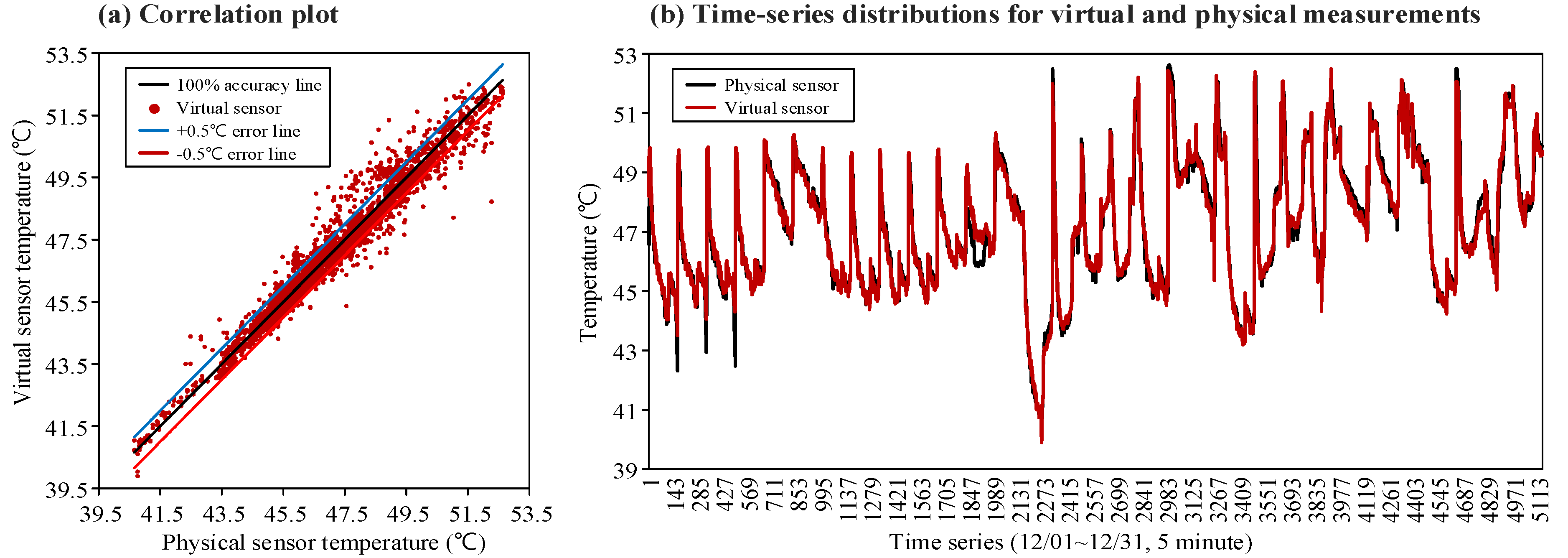
4.1. Measurements from IBVS

Figure 4 shows the daily RMSE distribution for the IBVS of $T_{DM,ret}$ during the entire operation period (47 days). Compared to the RMSE in the development period, the daily RMSE showed greater values of less than 1.0 °C. The average daily RMSE was 0.56 °C. Even though smaller errors occurred on certain days, such as January 24 and 26, and the average RMSE was acceptable, considerable errors of higher than 0.8 °C were found on six days. These results show the operational in situ virtual sensor errors caused by the various uncertainties of working environments in a real system. This indicates the necessity of calibrating operational virtual sensors in the energy systems of buildings.

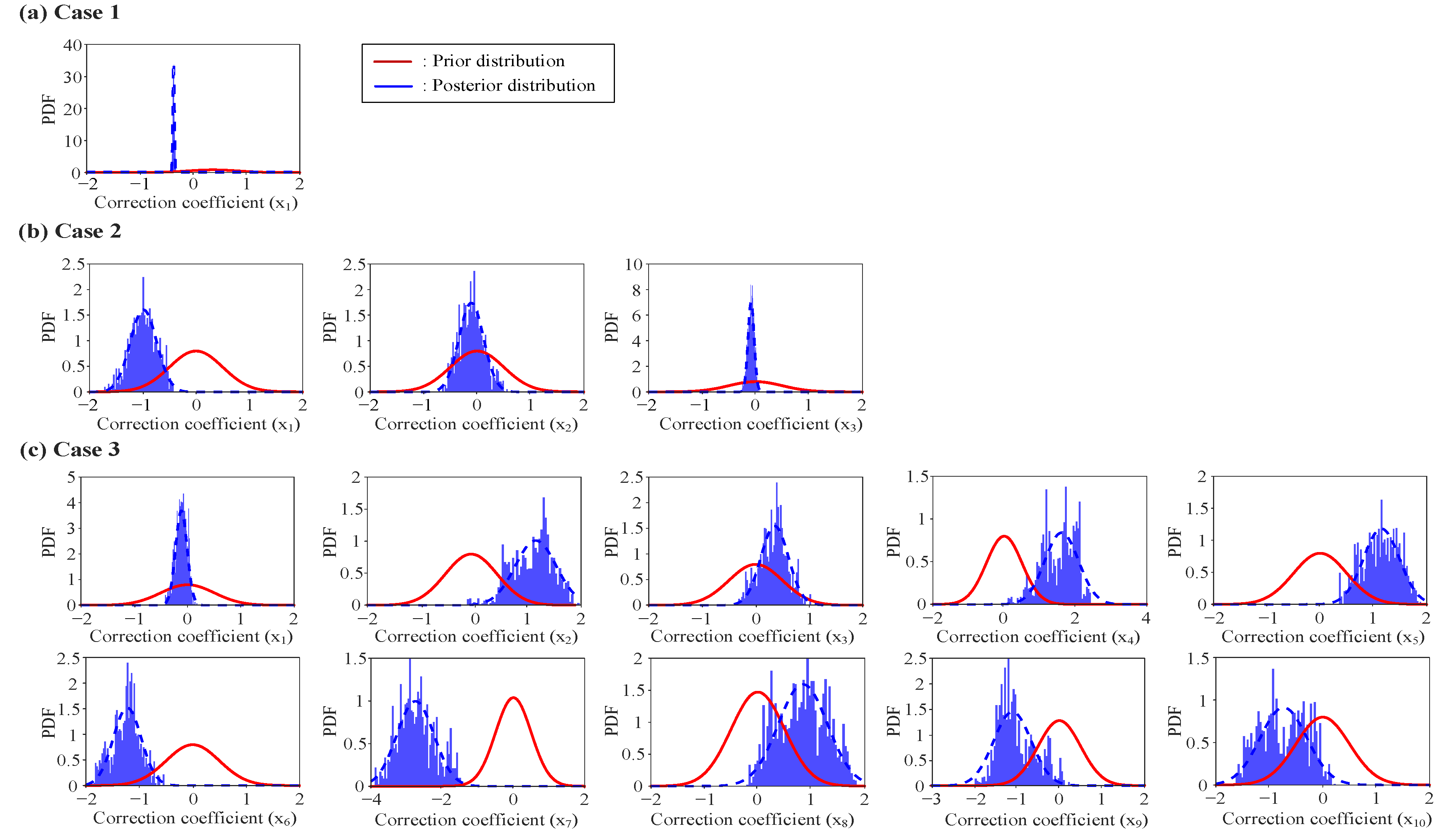
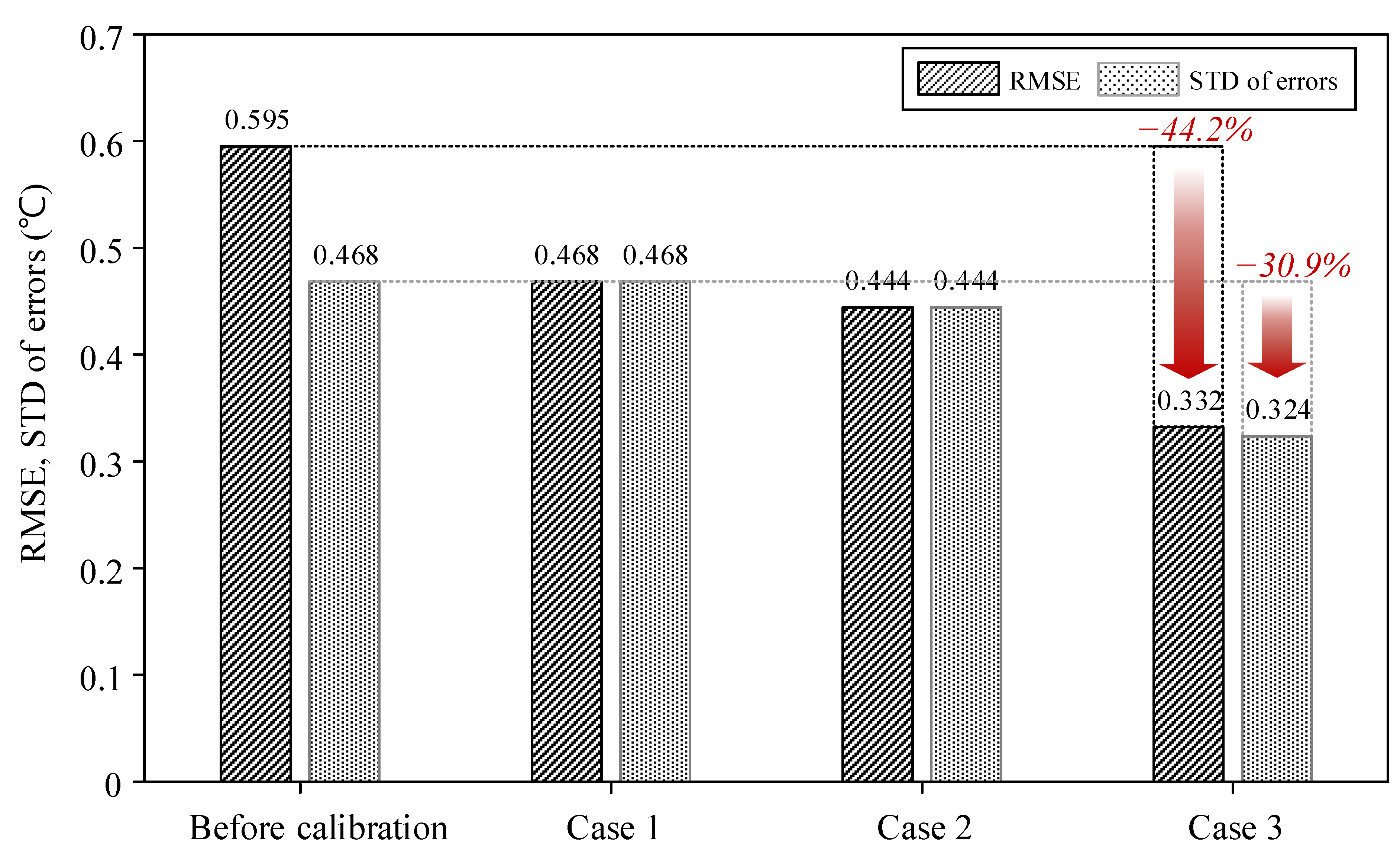
4.2. Calibrated Backup Virtual Sensors

According to the virtual sensor performance, as shown in Figure 4, VIC was applied for the calibration period to focus more on the characteristics of various error distributions. The VIC results were suggested for each calibration case, as shown in Figure 5. Using the defined correction functions, the virtual sensor accuracy can be improved after calibration in all three cases. In Cases 1 and 2, the RMSE was slightly decreased compared to that observed in the initial development, and a low RMSE of 0.332 °C was determined in Case 3. Compared to the virtual sensor accuracy before calibration (0.595 °C), the three cases were considered to be successful calibrations with reasonable acceptance ratios, as in Table 4, in the Bayesian MCMC process.

Figure 6 shows the virtual sensor measurements, according to the particular case during operation, after calibration. All cases showed better performance in terms of bias and random error types, as shown in Figure 7. However, Case 2 did not show great improvement. This was because the correction functions with the output variable were not suitable for representing the features of the operational virtual sensor errors. On the other hand, Case 3 demonstrated the best agreement with the physical measurements during the validation period. Considering the difference between the correction functions in Cases 2 and 3, the physical measurements for the operational input variables (V) in Equation (4) were key to providing a successful calibration performance, rather than using the output variables directly. Even though the performance of Case 1 was better than Case 2, the correction constant was not enough to calibrate the virtual sensor errors changing in operation.

Finally, the virtual sensor performance was compared with the calibration cases, using RMSE and standard deviations in the error distribution for the validation period (February 2021), as shown in Figure 7. Case 3 could decrease the IBVS error by 22.7% and 18.7% from the perspective of sensor error types, such as bias and random error, respectively. Particularly in the case of the three days (17–19 February) with higher errors, the IBVS was improved by 50.1% and 22.5% for bias and random error, respectively. The RMSE of 0.42 °C in a month can be regarded as showing a highly accurate virtual sensor, considering (1) the virtual temperature accuracies (mean absolute errors), ranging from 0.4 °C to 1.8 °C in the validation periods within 17 days, as suggested in the existing study [15], and (2) the training RMSE of 0.40 °C, as shown in Figure 2. This case study demonstrates the capability of the proposed VIC method for constructing reliable virtual sensing environments in operational building systems.

5. Conclusions

In this study, we proposed a VIC method for IBVSs in operational building systems. The case study showed the application results, which highlighted the operational errors of the IBVS, the necessity of calibrating virtual sensors, and the improvements achieved using the proposed calibration method. According to the results of this application, the initial backup virtual sensor for the heating water return temperature had a daily RMSE of 0.97 °C at its worst, and the proposed method seen in Case 3 could provide a lower RMSE of 0.42 °C for the operation after calibration (as seen in February 2021) by correcting the operational uncertainties in a system. It was necessary for VIC to be formulated using the proper correction functions for predicting and offsetting the operational errors. Defining a correction function using a polynomial expression with related system variables is recommended, based on the findings of this study. Using these findings, the recommendation for correction functions and the proposed problem formulation regarding distance functions, correction functions, and Bayesian inference, the VIC for IBVSs can be applied to other operational building systems. This VIC for virtual sensors can contribute to establishing reliable virtual sensing environments, thus enhancing the effectiveness of virtual sensing applications in the energy systems of intelligent buildings.

Future studies regarding in situ virtual sensor calibration are necessary to establish the calibration optimization process by which the best timings of calibration, formulation of correction functions, and calibration period can be determined automatically. A VIC for multiple virtual sensors and dependent physical sensors is also a necessity in the energy systems of buildings.

References

1. Li, H.X.; Gül, M.; Yu, H.; Awad, H.; Al-Hussein, M. An energy performance monitoring, analysis and modelling framework for NetZero Energy Homes (NZEHs). Energy Build. 2016, 126, 353–364. [Google Scholar] [CrossRef]
2. Xiao, F.; Zhao, Y.; Wen, J.; Wang, S. Bayesian network based FDD strategy for variable air volume terminals. Autom. Constr. 2014, 41, 106–118. [Google Scholar] [CrossRef]
3. Ma, Z.; Yan, R.; Li, K.; Nord, N. Building energy performance assessment using volatility change based symbolic transformation and hierarchical clustering. Energy Build. 2018, 166, 284–295. [Google Scholar] [CrossRef]
4. Lee, T.; Yoon, S.; Won, K. Delta-T-based operational signatures for operation pattern and fault diagnosis of building energy systems. Energy Build. 2022, 257, 111769. [Google Scholar] [CrossRef]
5. Afram, A.; Janabi-Sharifi, F. Theory and applications of HVAC control systems—A review of model predictive control (MPC). Build. Environ. 2014, 72, 343–355. [Google Scholar] [CrossRef]
6. Zhao, Y.; Zhang, C.; Zhang, Y.; Wang, Z.; Li, J. A review of data mining technologies in building energy systems: Load prediction, pattern identification, fault detection and diagnosis. Energy Built Environ. 2020, 1, 149–164. [Google Scholar] [CrossRef]
7. Yu, D.; Li, H.; Yu, Y.; Xiong, J. Virtual calibration of a supply air temperature sensor in rooftop air conditioning units. HVAC R Res. 2011, 17, 31–50. [Google Scholar] [CrossRef]
8. Li, H.; Yu, D.; Braun, J.E. A review of virtual sensing technology and application in building systems. HVAC R Res. 2011, 17, 619–645. [Google Scholar] [CrossRef]
9. Bellanco, I.; Fuentes, E.; Vallès, M.; Salom, J. A review of the fault behavior of heat pumps and measurements, detection and diagnosis methods including virtual sensors. J. Build. Eng. 2021, 39, 102254. [Google Scholar] [CrossRef]
10. Yu, Y.; Li, H. Virtual in-situ calibration method in building systems. Autom. Constr. 2015, 59, 59–67. [Google Scholar] [CrossRef] [Green Version]
11. Yoon, S.; Yu, Y. Extended virtual in-situ calibration method in building systems using Bayesian inference. Autom. Constr. 2017, 73, 20–30. [Google Scholar] [CrossRef] [Green Version]
12. Ploennigs, J.; Ahmed, A.; Hensel, B.; Stack, P.; Menzel, K. Virtual sensors for estimation of energy consumption and thermal comfort in buildings with underfloor heating. Adv. Eng. Inform. 2011, 25, 688–698. [Google Scholar] [CrossRef]
13. Yoon, S.; Choi, Y.; Koo, J.; Hong, Y.; Kim, R.; Kim, J. Virtual Sensors for Estimating District Heating Energy Consumption under Sensor Absences in a Residential Building. Energies 2020, 13, 6013. [Google Scholar] [CrossRef]
14. Kim, R.; Hong, Y.; Choi, Y.; Yoon, S. System-level fouling detection of district heating substations using virtual-sensor-assisted building automation system. Energy 2021, 227, 120515. [Google Scholar] [CrossRef]
15. Cotrufo, N.; Zmeureanu, R.; Athienitis, A. Virtual measurement of the air properties in air-handling units (AHUs) or virtual re-calibration of sensors. Sci. Technol. Built Environ. 2019, 25, 21–33. [Google Scholar] [CrossRef]
16. Choi, Y.; Yoon, S. Virtual sensor-assisted in situ sensor calibration in operational HVAC systems. Build. Environ. 2020, 181, 107079. [Google Scholar] [CrossRef]
17. Yoon, S. In-situ sensor calibration in an operational air-handling unit coupling autoencoder and Bayesian inference. Energy Build. 2020, 221, 110026. [Google Scholar] [CrossRef]
18. Li, M.; Lu, Q.; Bai, S.; Zhang, M.; Tian, H.; Qin, L. Digital twin-driven virtual sensor approach for safe construction operations of trailing suction hopper dredger. Autom. Constr. 2021, 132, 103961. [Google Scholar] [CrossRef]
19. Choi, Y.; Yoon, S. Autoencoder-driven fault detection and diagnosis in building automation systems: Residual-based and latent space-based approaches. Build. Environ. 2021, 203, 108066. [Google Scholar] [CrossRef]
20. Yu, Y.; Yoon, S. Hidden factors and handling strategies on virtual in-situ sensor calibration in building energy systems: Prior information and cancellation effect. Appl. Energy 2018, 212, 1069–1082. [Google Scholar] [CrossRef]
21. Yu, Y.; Yoon, S. Hidden factors and handling strategy for accuracy of virtual in-situ sensor calibration in building energy systems: Sensitivity effect and reviving calibration. Energy Build. 2018, 170, 217–228. [Google Scholar] [CrossRef]
22. Yoon, S.; Yu, Y. Strategies for virtual in-situ sensor calibration in building energy systems. Energy Build. 2018, 172, 22–34. [Google Scholar] [CrossRef]
23. Wang, P.; Han, K.; Liang, R.; MA, L.; Yoon, S. The virtual in-situ calibration of various physical sensors in air handling units. Sci. Technol. Built Environ. 2021, 27, 691–713. [Google Scholar] [CrossRef]
24. Liu, Z.; Huang, Z.; Wang, J.; Yue, C.; Yoon, S. A novel fault diagnosis and self-calibration method for air-handling units using Bayesian Inference and virtual sensing. Energy Build. 2021, 250, 111293. [Google Scholar] [CrossRef]
25. Wang, P.; Li, J.; Yoon, S.; Zhao, T.; Yu, Y. The detection and correction of various faulty sensors in a photovoltaic thermal heat pump system. Appl. Therm. Eng. 2020, 175, 115347. [Google Scholar] [CrossRef]
26. Dixon, P.; Ellison, A.M. Bayesian inference: Introduction. Ecol. Appl. 1996, 6, 1034–1035. [Google Scholar] [CrossRef]
27. Aksu, G.; Güzeller, C.O.; Eser, M.T. The Effect of the Normalization Method Used in Different Sample Sizes on the Success of Artificial Neural Network Model. Int. J. Assess. Tools Educ. 2019, 6, 170–192. [Google Scholar] [CrossRef] [Green Version]
28. Metropolis, N.; Rosenbluth, A.W.; Rosenbluth, M.N.; Teller, A.H.; Teller, E. Equation of state calculations by fast computing machines. J. Chem. Phys. 1953, 21, 1087–1092. [Google Scholar] [CrossRef] [Green Version]
29. Hastings, W.K. Monte carlo sampling methods using Markov chains and their applications. Biometrika 1970, 57, 97–109. [Google Scholar] [CrossRef]
Figure 1. Diagram of the target heating system.
Energies 15 01394 g001
Figure 2. Accuracy of the target virtual sensor during the development period (December 2020).
Energies 15 01394 g002
Figure 3. Priors and posteriors for the three calibration cases.
Energies 15 01394 g003
Figure 4. The daily RMSE distribution of the target virtual sensor in the whole operation period.
Energies 15 01394 g004
Figure 5. Comparison of the RMSEs of the three calibration cases for the calibration period.
Energies 15 01394 g005
Figure 6. Virtual sensor measurements before and after all calibration cases throughout the entire operation.
Energies 15 01394 g006
Figure 7. Comparison of virtual sensor performance, displayed according to cases, for the validation period (February 2021).
Energies 15 01394 g007