Abstract
Hydropower is the most widely used renewable power source worldwide. The current work presents a methodological tool to determine the hydropower potential of a reservoir based on available hydrological information. A Bayesian analysis of the river flow process and of the reservoir water volume is applied, and the estimated probability density function parameters are integrated for a stochastic analysis and long-term simulation of the river flow process, which is then used as input for the water balance in the reservoir, and thus, for the estimation of the hydropower energy potential. The stochastic approach is employed in terms of the Monte Carlo ensemble technique in order to additionally account for the effect of the intermediate storage retention due to the thresholds of the reservoir. A synthetic river flow timeseries is simulated by preserving the marginal probability distribution function properties of the observed timeseries and also by explicitly preserving the second-order dependence structure of the river flow in the scale domain. The synthetic ensemble is used for the simulation of the reservoir water balance, and the estimation of the hydropower potential is used for covering residential energy needs. For the second-order dependence structure of the river flow, the climacogram metric is used. The proposed methodology has been implemented to assess different reservoir volume scenarios offering the associated hydropower potential for a case study at the island of Crete in Greece. The tool also provides information on the probability of occurrence of the specific volumes based on available hydrological data. Therefore, it constitutes a useful and integrated framework for evaluating the hydropower potential of any given reservoir. The effects of the intermediate storage retention of the reservoir, the marginal and dependence structures of the parent distribution of inflow and the final energy output are also discussed.
1. Introduction
Hydropower is a clean, renewable source of energy that significantly contributes to the reduction of greenhouse gas emissions; however, global warming is expected to have an impact on water availability and thus on hydropower management. Hydropower generation in the Mediterranean region has mainly been developed on the mainland due to the hydropower potential provided by large rivers and lakes. At the same time, several Mediterranean islands are not connected to the main electricity grid (e.g., [1]), meaning that independent local grids cater for their power requirements, mainly using imported fossil fuels, contributing to global warming. Seasonal variability in power demand, fuel price volatility, as well as growing tourism development, impose additional complexity [2]. Over the past couple of decades, the EU has funded the construction of several dams and reservoirs for water supply and irrigation purposes in islands such as Cyprus, Crete, Sicily, Corsica and Majorca. In some cases, the exploitation of the hydroelectric potential, respecting the islands’ water needs and a multipurpose use of the reservoirs, has been a topic of investigation as it could contribute to a sustainable energy system and support the implementation of the revised Renewable Energy Directive (2018/2001/EU). Spain, Italy and France produce over 20 GW from hydropower, while Greece only produces 3.4 GW [3,4]. Small hydropower plants can play a major role in improving energy autonomy and contributing to renewable energy and the climate neutrality agenda as hydropower is considered one of the most sustainable and clean energy sources in terms of carbon emissions [5,6,7]. The assessment of the hydropower potential on islands such as Crete would be a very effective tool for local stakeholders allowing them to acquire funding from private and public sectors for hydroelectric power production.
On the island of Crete, there are five reservoirs of approximately 20 Mm3 capacity in total, and an additional one is under construction. The reservoirs have recently become operational, and a balanced surface water–groundwater use is planned for the efficient management of the reservoir resources. The Region of Crete has often considered incorporating small hydropower plants in existing hydraulic projects—in certain locations selected as suitable for multipurpose water uses (e.g., irrigation, water supply, hydropower)—and has set as a target in its recent Water Resources Management Plan for the island: the assessment of the hydropower potential of existing reservoirs [8,9]. In view of the above, the main motivation and objective of this study is to develop and propose a methodological tool for analyzing river inflows and the water balance of multipurpose reservoirs in order to estimate the potential for small hydropower development, while respecting irrigation, water supply needs or both, and thus contribute to increasing the share of renewable energy resources on Mediterranean islands.
The topic has been addressed in numerous previous works presenting various methodologies to estimate hydropower potential and identify suitable hydropower sites. For example, ref. [10] applied river-basin-scale distributed hydrological modelling and GIS tools; ref. [11] used remote sensing and streamflow data processed through GIS-based tools to identify potential hydropower production locations; ref. [12] estimated the maximum potential hydropower production in La Plata basin under demographic and hydrological changes by employing a GIS numerical tool integrating hydrologic, physiographic, economic and social data; ref. [13] presented a GIS-based methodology for identifying suitable locations for hydropower production based on digital elevation and river discharge maps; ref. [14] analyzed numerous sites in Brazil for potential run-of-river hydroelectric plants, using python scripts and QGIS for generating multiple regression models for river flows, flooded areas and estimates of hydropower potential. A global scale assessment of the technical and economic potential of hydropower, using cost optimization methods, was performed by [15], while similarly, the economic feasibility of multi-reservoir hydropower systems was addressed by [16], who developed a simulation-optimization model for optimal design of hydroelectric production systems. The hydropower potential under climate change has been studied, for example, in [17,18,19,20], combining hydrological modelling and downscaled meteorological output from general circulation models (GCMs).
Analysis of inflows and the reservoir water balance, for developing and applying optimal reservoir operation models, is the key to optimizing hydropower production and increasing the percentage of renewable energy resources. In multi-purpose reservoirs, a Bayesian approach can be a useful tool for analyzing the water balance as a typical risk–benefit problem in water resources management [21,22], given that water supply, hydropower production and environmental water use are conflicted water uses linked by water inflows in the basin. A joint analysis method, the copula method, as well as multivariate distribution functions, are also useful tools to involve these dependences in water resources systems [23,24]. Chen et al. (2020) [24], for example, analyzed the water supply, hydropower production and environmental water nexus based on the multivariate distribution functions by establishing joint distributions and conditional expectation models to evaluate risks in the water resources system.
To address the uncertainties in streamflow estimation and forecast, implicit or explicit stochastic optimization is employed in developing reservoir operation models. Implicit stochastic optimization refers to deterministic optimization methods, such as genetic programming, particle swarm optimization and discrete differential dynamic programming to extract the reservoir operation rules using linear regression (e.g., [25,26,27]), whereas in explicit stochastic optimization, reservoir inflow is considered a stochastic process described by probability distributions, and streamflow uncertainty is integrated into the reservoir operation model [28,29,30,31]. Bayesian theory is often used in these models to incorporate transition probabilities, including prior, likelihood and posterior probabilities, for quantifying water inflow uncertainties (e.g., [31,32]). In [31], an explicit expression of the conditional probability is derived based on copula functions, which is then used to calculate prior and likelihood probabilities, and the prior probability can be updated to the posterior probability (when new inflow forecast is available) using the Bayesian formulation. Different models for reservoir operation are in many cases combined by using Bayesian Model Averaging [33] in order to reduce uncertainty in estimations and improve decision making. For example, ref. [34] combined three different reservoir operation models with Bayesian Model Averaging to reduce the uncertainty of reservoir operating rules. To assess the impacts of climate change, reservoir operation models adaptive to non-stationary inflow conditions have been developed (e.g., [35,36]). Yang et al. (2021) [36], for example, proposed a Bayesian-based adaptive reservoir operation framework to increase the reliability for power generation, incorporating streamflow non-stationarity under climate change, by using Bayesian Model Averaging [33].
In the current study, a methodological framework is proposed that can assess, in a systematic manner, the hydropower potential of a reservoir, considering the water supply and residential energy demands. The proposed tool determines the hydropower potential following a stochastic approach and is applied to the Faneromeni reservoir on the island of Crete, Greece. It can be easily relocated to other Mediterranean islands facing similar challenges. The tool’s innovations lie on the combination of two methodological approaches to estimate the hydropower potential under river flow realization uncertainty, proposing an explicit methodology for retaining the parent probability density function form and the second order dependence structure of the river flow across scales. A Bayesian analysis of the river flow and available water volume in the reservoir is applied, and the estimated probability density function parameters are integrated for a stochastic analysis and long-term simulation of the river flow process, which is then used as input for the water balance in the reservoir, and thus, for the estimation of the hydropower residential energy potential. In more detail, the probability of critical reservoir volumes occurring due to hydropower generation and the associated uncertainty are determined through Bayesian analysis, which calculates the posterior probability distribution of streamflow and reservoir water volume variations. The stochastic analysis is applied in terms of the Monte Carlo ensemble technique. A synthetic river flow timeseries is first simulated by preserving the marginal probability distribution function properties of the observed timeseries and also by explicitly preserving the second-order dependence structure (e.g., autocorrelation function) of the river flow. Next, the synthetic ensemble is used for the simulation of the reservoir water balance, and finally, for the estimation of the hydropower potential for covering residential energy needs. For the second-order dependence structure of the river flow, the climacogram metric is used (expressed in the standard deviation, instead of the variance, of the averaged process vs. scale; [37]), which is shown to have a lower statistical bias compared to other common stochastic tools such as the autocovariance function and the power-spectrum [38].
In previous studies, the stochastic simulation of the water balance in the reservoir, and in particular, of the input streamflow, is performed by preserving the marginal structure of the process (e.g., [39,40,41,42] or by applying a transformation from the Gaussian parent distribution to the desired parent distribution in order to implicitly preserve the marginal distribution and the autocorrelation structure through autoregressive models (e.g., [43,44,45,46,47,48]). Here, we use an algorithm that can explicitly preserve an adequate and necessary number of moments from the marginal function of the gamma distribution and the second-order Hurst-Kolmogorov dependence structure, as identified and expressed through the less statistical biased metric of the climacogram, for a vast range of scales ([49]; for the merits of this method and applications of explicit preservation of four to six marginal moments, see [50]. For the preservation of as many required moments, see [51]).
The paper is structured as follows: in Section 2, the study and methodology are presented, providing a detailed description of the Bayesian and stochastic approaches applied and the set of equations used for estimating the hydropower generation potential of the reservoir; in Section 3, results of the application of the methodological framework to the study area reservoir are presented, and the main findings and limitations of the current work are discussed; Section 4 presents the main conclusions.
The proposed tool can serve as a Decision Support System to assess the optimal hydropower production potential of the reservoir according to its capacity, the irrigation needs of the surrounding areas and the hydrological characteristics of the study area.
2. Materials and Methods
2.1. Study Area
The case study reservoir is located on the island of Crete, Greece, and more specifically in the south of the island, in the Geropotamos river basin (Figure 1). The irrigation needs of the area are high, while the primary source of water is groundwater. Since 2013, a reservoir with an effective storage volume of 17.86 hm3 (Table 1) is operating in the area in order to contribute towards meeting the water demand and reducing the dependence on groundwater [8]. The reservoir is connected to an irrigation network to cover the needs of the most productive part of the valley that requires 5 hm3/year of water. Recent literature includes many works studying the water resources management of the area, including the reservoir potential, considering climate variability scenarios [21,22,52,53,54]. The reservoir is located at an elevation of 209 m and receives the runoff of the nearby Koutsoulidis river. The hydrological potential and characteristics of the reservoir are assessed using statistical approaches examining two different datasets. The first considers the reservoir’s daily volume data since 2016, while the second considers the daily average river flowrate that has fed the reservoir since 1975 [55]. A Bayesian analysis is first employed, while a stochastic simulation method, based on the Monte Carlo technique of including information from both datasets, is applied in advance.
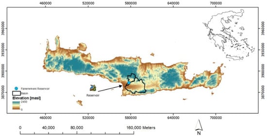
Figure 1.
Study area and location of the reservoir.

Table 1.
Faneromeni Reservoir characteristics.
2.2. Methodology
As described briefly in the introduction section, the potential of the reservoir for hydropower production is estimated by employing a Bayesian and a stochastic analysis of streamflow, which is then used for calculating the water balance of the reservoir, and thus, for the estimation of the hydropower potential. Specifically, the first step is the fitting of the marginal probability distribution function on the observed timeseries. Secondly, the posterior probability distribution of streamflow and reservoir water volume variations is estimated. Herein, the Bayesian method output is incorporated into a stochastic approach in terms of Monte Carlo simulations preserving the necessary number of moments of the marginal probability and second-order dependencies structures to simulate the river flow rate and the reservoir water balance under uncertainty, and finally, the last step is the estimation of the hydropower potential. An overview of the methodology applied and the reservoir schematic are shown in Figure 2. A detailed presentation of the aforementioned methodological steps is provided in the following paragraphs.
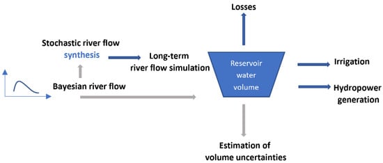
Figure 2.
Schematic representation of the reservoir and the applied methodology.
2.2.1. Net Power Estimation
The actual power obtainable from the hydropower scheme considers head loss and turbine, generator, gearbox and transformer efficiency following the proposed guide from the European Small Hydropower Association [56]. The net head is the gross head (H) subtracting the frictional losses (hf). The net power is calculated as:
where P is the net power in [W], Q is the flow rate in [m3/s] through the turbine, Hn is the net head in [m], nturbine is the efficiency of the turbine, ngenerator is the efficiency of the generator, ngearbox is the efficiency of the gearbox, ntransformer is the efficiency of the transformer and w is the specific weight of water (9.81 KN/m3). Using Manning’s equation for a closed pipe of circular cross-section, frictional losses are calculated as:
where L is the length of the pipe, hf is the frictional loss (head loss), J is the hydraulic gradient, D is the diameter of the circular pipe, Q is the flowrate through the pipe (penstock) and n is Manning’s coefficient (e.g., Welded steel is taken as 0.012). The rate of flow in the penstock is calculated using a modified equation according to [56], limiting the loss of power to 4%. This is illustrated through the equation:
Note that the diameter, d, of the dam’s intake or gate depends on the flowrate Q and is calculated using the equation:
where is the gravity acceleration and H is the gross head.
2.2.2. Bayesian Approach
The hydrological potential of the reservoir is examined by fitting established marginal distributions to the river flow process and to the water volume in the reservoir.
where f(p) is the probability density function (Table 2) and up or F(P) is the corresponding cumulative distribution function. The tested probability distribution functions are shown in Table 2.
Table 2.
Commonly used distributions in hydrology.
In order to evaluate the performance of the univariate marginal distributions, the empirical probability is estimated in terms of the Weibull plotting position equation:
where Xi is observed data, N is the sample size and Femp (Xi) is the empirical exceedance probability of the ith observed data Xi [57].
The performance evaluation of the marginal distributions F(xi), is applied using the Root Mean Square Error (RMSE), , the difference of actual observations, , and estimations, , under sample size N and the Akaike Information Criterion (AIC), AIC = −2ln(Lm) + 2K, where Lm is the maximum value of the likelihood function of the model and K is the number of estimated parameters [58].
The statistical properties of the daily volume of the reservoir and of the average daily river flow rate are examined by fitting the aforementioned probability distributions. The values of the distribution parameters depend on the structure of the sample timeseries. Therefore, it is reasonable to assume that the parameters’ prior distribution follows a probability distribution that depends on the sample records. Using a Bayesian approach, the parameters are calculated in terms of a probability distribution by means of the impact of the sample.
Specifically, a Bayesian approach involves the prior distribution of the model parameters expressed through the vector θ:
The parameters are estimated in a Bayesian framework, wherein the posterior distribution of θ is sought, e.g., the conditional distribution of θ given the data Yobs, , which can be expressed using Bayes’ rule as follows:
where is the likelihood function for the observed data given the parameters and p(θ) is the prior joint distribution of the parameters. Assuming independence of the prior distributions of the parameters, the prior joint distribution of parameters factors into the product of the prior distributions, and the posterior density simplifies to:
The posterior distributions of the parameters are obtained from Equation (9) [59].
2.2.3. Stochastic Approach
The stochastic approach is applied in terms of the Monte Carlo ensemble technique. A synthetic river flow timeseries is first simulated by preserving the marginal probability distribution function properties of the observed timeseries and also by preserving the second-order dependence structure of the river flow through the autocorrelation function. Next, the synthetic ensemble is used for the simulation of the reservoir water balance, and finally, for the estimation of the hydropower potential for covering residential energy needs.
For the second-order dependence structure of the river flow the climacogram metric is used (i.e., standard deviation of the averaged process vs. scale) [37], which is shown to have a lower statistical bias compared with other common stochastic tools, such as the autocorrelation function and the power-spectrum [38], and is based on the theoretical value of the selected stochastic model.
For example, the climacogram model for the most common power-type autocorrelation function of the fractional-Gaussian-noise (fGn), is:
where λ = σ is the standard deviation of the river flow process and Hu is the Hurst [60] parameter, which for the white-noise model is Hu = 0.5 and for a long-term persistent process is 0.5 < Hu < 1.
For the stochastic generator of the synthetic river flow timeseries, , the Symmetric-Moving-Average scheme (SMA; [61]) is used, which can preserve exactly the second-order dependence structure, as identified through the climacogram, and the marginal distribution function through the method of joint-moments [49]:
where αj are coefficients that can be calculated if the climacogram expression is known. For example, for the climacogram shown in Equation (10), the coefficients are estimated as:
Furthermore, determines the number of the coefficients that are needed and is usually taken to be equal to the length of the produced timeseries. Finally, is a white-noise process that is used to preserve the marginal structure of the process. For example, for fGn, follows a Gaussian distribution, whereas for non-Gaussian distributions of the parent process, a heavy-tailed distribution can be applied [50,51].
Then, the mean annual water volume in the reservoir, V, can be estimated for each annual time step by implementing the expression:
where is the percentage of streamflow, S(t), that actually reaches the reservoir, A is the annual water volume that is extracted from the reservoir for agricultural purposes and Vmax is the maximum capacity of the reservoir.
Finally, the produced hydroelectric energy that is to be used for the residential energy demand, E(t), is estimated from the expression below, as derived accordingly to the previous section:
where nt is the total efficiency of the turbine and Ta is the working hours of the turbine.
Note that to transform the water volume to water level in the reservoir, a relationship between the available water volume, V, and the water level, H, can be defined to support the simulation process:
3. Results and Discussion
Following the methodology described in the previous section, the hydropower potential for the case study reservoir is calculated using the average supply volume of the reservoir that corresponds to 6.127 hm3 or 17.8 m of water level as a pilot example. In the following paragraphs, results from each approach are presented and discussed.
3.1. Evaluation of Hydraulic Parameters for the Case Study
Input of the following parameters, H = 17.8 m, L = 150 m, n = 0.012 (Welded steel pipe), D = 1.2 m into Equation (3) and results in a flow rate equal to Q = 2.78 m3/s. Given that the friction losses increase as the length of the pipe increases, such diameter and length are chosen to reduce the frictional losses up to 4% and the flow rate.
The diameter of the intake or gate of the dam is calculated from Equation (4), where: Q = 2.78 m3/s, g = 9.81 m/s2, H = 17.8 m, resulting in an intake diameter equal to d = 0.45 m. To achieve low losses in the penstock (4%), the flowrate should be similarly low. Thus, to reduce the hydraulic gradient, a decrease in flow rate of 2.78 m3/s enables the use of a penstock pipe length of up to 150 m at a friction loss of 4% of static head. This is achieved by using a diffuser to reduce the velocity from the reservoir leading to the penstock pipe. Thus, the flow rate caused by the fall potential of the water from the reservoir is reduced to 2.78 m3/s in the penstock, so that losses in the penstock can be as low as 4%.
The gross head (H) equals the difference between the normal pool elevation (226.8 m) and the riverbed elevation (209 m) and is estimated to be equal to 17.8 m. From Equation (2), the head loss (hf) is estimated to be equal to 0.71 m (4% drop in the static head of 17.8 m), by taking L = 150 m, n = 0.012, Q = 2.78 m3/s and D = 1.2 m; hence, Hn = 17.09 m.
From Equation (1) and for Q = 2.78 m3/s, Hn = 17.09 m, nturbine = 0.94 (e.g., Kaplan turbine), ngenerator = 0.96 (industrial size turbine generators), ngearbox = 0.95, ntransformer = 0.96 and w = 9.81 kN/m3, the net power is estimated as P = 381.3 kW. Based on an average of 150 working days per year, the average annual energy in output of the hydro generator is calculated equal to 1,372,680 kWh/year.
The reservoir’s effective volume is 17,860,000 m3. The irrigation needs in the most productive part of the Messara valley at the Geropotamos river basin is around 5,000,000 m3/year. This means that annually, the optimum management of the reservoir requires the availability of this volume for the agricultural activities in the area.
The average reservoir level, since its operation began, is 17.8 m, which corresponds to a supply volume of 6,127,000 m3. Since 2016, when the reservoir was first fully operated, it has only been filled once, in 2019. Therefore, for the irrigation needs to be covered and the hydropower production to be feasible at the calculated level, at least 11,000,000 m3 (60% of the maximum reservoir volume) should be available every year. Obviously, lower amounts of hydropower energy can be produced that would require a smaller amount of water to be available.
According to the Greek national statistical authority, every Greek household consumes an average of 3750 kWh/year. This means that the hydropower facility in the Faneromeni area can cover up to 366 households per year. Estimating that there are, on average, four family members in each household, the previous calculation corresponds to almost 1470 inhabitants. This specific population number corresponds to 30% of the population of one of the most populated towns in the area (i.e., Moires and Tympaki) or to the entire population of the two villages close to the reservoir location (i.e., Voroi and Fanerwmeni).
Given that the electrical power in the area is transferred from the city of Heraklion using non-fossil fuels, an investment in hydropower production could provide a significant alternative to cover a significant part of the required electricity volume in the area.
3.2. Bayesian Approach
When the reservoir is full, the water volume available for hydropower production is around 12,860,000 m3, which according to the proposed methodology corresponds to a pool level of 28.17 m and a flow rate of 4.4 m3/s, and therefore, to a hydropower potential of 972 kW. On average, over 150 working days per year, the average annual energy output is 3,500,000 kWh/year, which is sufficient to cover the energy demand of up to 933 households or 3733 inhabitants, which corresponds to 30% of the municipality population.
For the hydropower potential to be analyzed based on realistic reservoir volumes, a Bayesian method is applied. As a base line scenario, it is considered that almost 60% of the reservoir volume is filled, which corresponds to a ‘baseline’ hydropower production equal to that originally calculated, while the potential of 75% (almost 13,500,000 m3) of the reservoir being filled is examined along with a full reservoir scenario. Any design scenario based on less than 60% of the reservoir capacity available requires an alternative water resources management scenario to cover the irrigation needs of the area. The second scenario examined (75% of the reservoir volume available) corresponds to a 680 kW hydropower potential or 2,448,895 kWh/year for an average of 150 working days per year, which can cover the energy demand of up to 653 households or 2612 inhabitants.
The sustainability of a hydropower production investment such as this is further examined based on a Bayesian statistical analysis. According to the results of Table 3, the best fitted probability distribution on the daily water volume in the reservoir, since 10 January 2016, is the Gamma distribution function. Thus, the parameters of the distribution should also follow a similar function. In this work, the ‘‘spBayes’’ library [62] in R is used for model fitting and the posterior parameters distribution calculation; it also provides their mean value and the 5th and 95th percentiles (Table 4).
Table 3.
Goodness-of-fit results of marginal distributions (reservoir volume).
Table 4.
Estimated parameters for best fitted marginal distribution (reservoir volume).
According to the calculated parameters, the probability of occurrence of the examined water volumes, that can be used for hydropower generation, is determined (Figure 3). Specifically, the probability that the reservoir will be filled to 60% capacity is 17%, with a lower boundary of 13% and an upper one of 29%, while the probability that the reservoir will be filled to 75% capacity is 9%, with a lower boundary of 6% and an upper boundary of 18%. The probability that the reservoir will be full is 3%, with a lower boundary of 1% and an upper boundary of 7%.
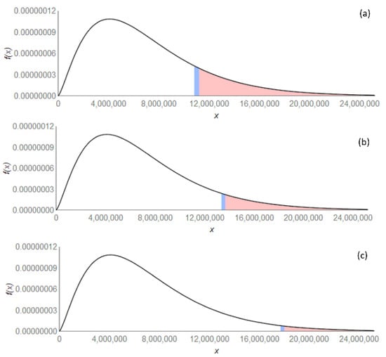
Figure 3.
Compound Gamma Probability distribution function of the reservoir water volume (x) providing the different f(x) values for the examined reservoir volumes: (a) 60%, (b) 75%, (c) 100% filled.
The statistical properties of the average daily volumetric flowrate of the main river that has been feeding the reservoir since 1975 is also examined by fitting the aforementioned probability distributions. The best fitted distribution is found to be the Gamma distribution (Table 5). Similarly, it assumed that the parameters’ prior distribution follows the probability distribution of the sample values. The mean of the posterior calculated parameters and their 5th and 95th percentiles are presented in Table 6.
Table 5.
Goodness-of-fit results of marginal distributions (river flow).
Table 6.
Estimated parameters for the best fitted marginal distribution (river flow).
Considering the determined parameters, the probability of a specific river flow rate to feed the reservoir for irrigation and hydropower generation is calculated as shown in Figure 4. Specifically, the probability that the reservoir is filled to 60% capacity (0.35 m3/s) is 44%, with a lower boundary of 19% and an upper boundary of 71%, while, for a 75% available capacity (0.43 m3/s) the calculated probability is 24%, with a lower boundary of 8% and an upper boundary of 50%. The probability that the reservoir is full (0.56 m3/s) is 7%, with 0.8% and 22% lower and upper boundaries, respectively.
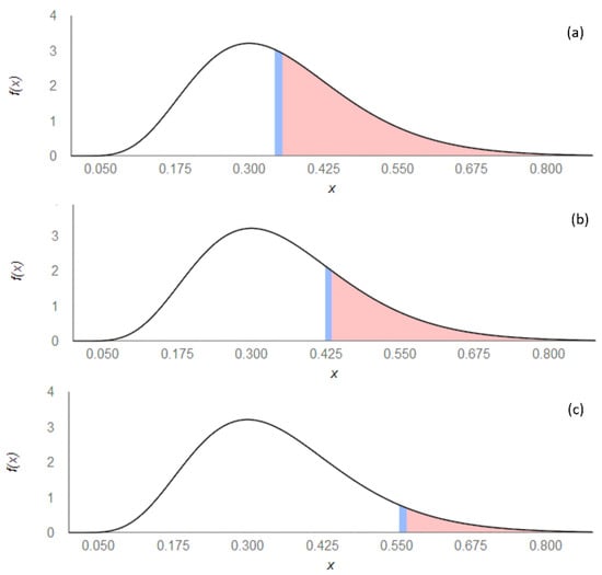
Figure 4.
Compound Gamma Probability distribution function of the river flow rate (x) providing the different f(x) values for the examined river flow rates to fill the reservoir by (a) 60%, (b) 75%, (c) 100%.
3.3. Stochastic Approach
The above two Bayesian analyses for the water volume inside the reservoir and the upstream river flow resulted in different values for the return period of the required water level for hydropower production. Therefore, a stochastic approach is also applied, based on the Monte Carlo ensemble technique, to include information from both datasets. A synthetic river flow timeseries of 1000 years is produced by preserving its marginal structure, as derived in the previous sections (i.e., the gamma probability distribution function), as well as its second-order dependence structure to account for the autocorrelation of the river flow process.
Moreover, additional information is used about the water losses inside the reservoir, and a simulation is performed for the water balance by accounting for the lower and upper water volume thresholds and the non-linear function between the water volume and the water level (Figure 5):
where V is the water volume (×106 m3) and H is the water level (m). The aim is to estimate, in this manner, the excess probability of the water volume and thus, to be able to decide on the available water volume for hydropower production as a function of the reliability and return period.
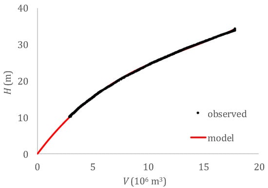
Figure 5.
Water volume vs. water level for the Faneromeni reservoir.
3.3.1. Stochastic Structure and Synthesis of the River Flow Process
The marginal structure for the river flow is analyzed in the above sections, where the gamma probability distribution, i.e., Γ (α, β) with α = 5.04 and β = 0.066 (μ = 0.33 m3/s and σ = 0.15 m3/s), is shown to have the most significant performance compared to other common tested distributions.
The estimated climacogram for the available river flow timeseries ranging from 1975 to 2019 (Figure 6) is best fitted by a white-noise process (i.e., all random variables of the river flow are independent of each other). However, this result may seem spurious given that it is rather unprecedented that future flows are completely independent of the past flows. In fact, it is shown that, in geophysical processes, a rather strong second-order dependence structure is found, which is characterized by a long-term persistent behavior [63].
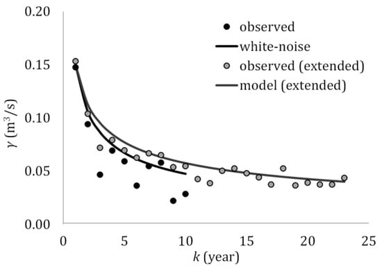
Figure 6.
Standard deviation of the averaged process vs. scale for the extended river flow timeseries upstream of the reservoir. Note that the climacogram is estimated up to the scale equal to 20% of the length of the timeseries as suggested to improve fitting in HK processes [38].
A possible reason for the above result may be that the sample length of the river flow is rather small, making the identification of any kind of dependence difficult to estimate from the data. Therefore, the extended river flow timeseries ranging from 2019 to 2099 is also included in the analysis, which is simulated with the RCP 2.6 scenario [54]. The climacogram of the latter extended timeseries exhibits a weak long-term persistent behavior, which is a stronger dependence structure than the white noise (WN) one (Figure 6). In this study, a stochastic simulation is performed for both cases, described through the second-order dependence structure expressed by the climacogram (Equation (11)) also called the Hurst-Kolmogorov process -HK-[49].
For the stochastic synthesis of the regular river flow process (Figure 7), we use the gamma probability distribution function, whereas for the extended flow process (Figure 6), we use the Symmetric-Moving-Average algorithm (Equation (11)) with following the gamma distribution Γ(κ,θ) with κ, θ:
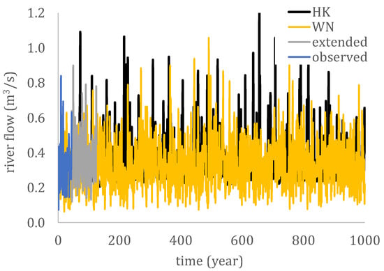
Figure 7.
The synthetic timeseries of 1000 years following a WN and HK processes, both with probability distribution function Γ(κ,θ).
3.3.2. Simulation of the Water Level Balance in the Reservoir
For the stochastic simulation of the mean annual water volume in the reservoir, V, a 1000-year-timeseries of mean annual streamflow, S, in the upstream river is produced, based on the aforementioned model. The 1000-year-length is selected so as to estimate, with high accuracy, the expected value of households that can be covered by the produced electricity from the reservoir. Then, from Equation (13), the mean annual water volume in the reservoir is estimated for each annual time step. Note that in the balance expression, any inflows or outflows from the precipitation and evapotranspiration of the reservoir are omitted, and all other losses (e.g., emergency outflows, reservoir losses etc.) are attributed to the streamflow losses through the parameter as shown in Equation (13).
From the previous sections, Vmax = 17.86 × 10⁶ m3, while the irrigation requirements are assumed to be fixed, i.e., A = 5 × 10⁶ m3/year. The annual losses of streamflow to the reservoir are also assumed to be fixed and can be estimated by minimizing the error between the average mean annual water level in the reservoir, which is set at 17.8 m as mentioned in the previous sections, and the one produced by the simulation (Figure 8). The water level in the reservoir for each time step, H(t), is easily obtained from Equation (16); hence, we find from the optimization that = 0.46, i.e., 54% of the streamflow corresponds to the reservoir water losses. The produced hydroelectric energy for residential energy demand, E(t), is then estimated from Equation (14) (see Figure 9 for the synthetic timeseries).
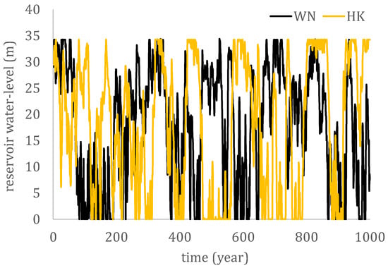
Figure 8.
Stochastic simulation of the annual mean water level in the reservoir for the WN and HK streamflow processes.
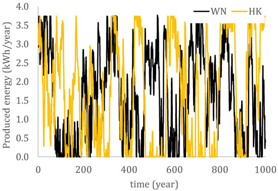
Figure 9.
Stochastic simulation of the produced residential energy for the WN and HK streamflow processes.
The average number of households that can be supplied with electricity by the hydroelectric dam can be estimated from the above stochastic simulation. It is estimated that 433 households can be supplied for the WN scenario and 454 households for the HK scenario. Comparison with the Bayesian approach, which estimates that 366 households can be supplied with electricity for the scenario of average reservoir supply volume, shows that the two different approaches provide close results. Compared with the 653 households calculated with the Bayesian methodology for maximum reservoir supply volume, the number of households calculated with the stochastic approach is smaller. In the real-time stochastic simulation, the thresholds of the reservoir, i.e., the maximum and minimum (i.e., zero) effective volume, are also taken into account. Therefore, it is expected that water volume is lost when the water level exceeds the one that corresponds to the maximum water volume of the reservoir and that the hydroelectric dam fails to supply the households with electricity when the reservoir is emptied. The probability for the first (overtopping) and the second (empty reservoir) failure is estimated as 3.8% and 12.4% for the WN scenario, and as 10.8% and 17.8% for the HK scenario, respectively.
To further illustrate this, we construct the probability distribution of the streamflow process and the empirical probability distribution of the produced energy from the simulation of both scenarios (WN and HK). It can be observed (Figure 10) that although the input of the stochastic simulation (i.e., streamflow) is gamma distributed, the output (i.e., produced energy) curvature of the probability distribution function is small, approximating the uniform distribution for both scenarios with a probability distribution function:
where E > 0 is the produced energy from the hydroelectric dam and a and b are model parameters, which for the stochastic simulation are estimated to be a = 0.658 × 10⁶ kWh/year, so that there is a probability at zero (i.e., E = 0) equal to the average probability of the second failure (i.e., (12.4% + 17.8%)/2 = 15.1%). b = 3.7 × 10⁶ kWh/year, which corresponds to the maximum produced energy at the maximum water level of the reservoir.
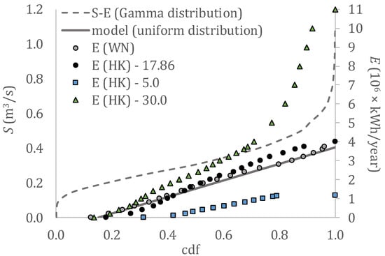
Figure 10.
The probability distribution functions from the stochastic simulation of the streamflow and the produced residential energy for the WN and HK scenarios with effective storage volumes of 17.86 (original), 5 (small size) and 30 (large size) hm3.
A similar observation is drawn from the second-order dependence structure of the input and output (Figure 11 and Figure 12), where although the input climacogram corresponds to a white-noise and Hurst-Kolmogorov process, the output climacogram can be approximated for both scenarios with a Markov model expressed through the generalized-HK (GHK) climacogram:
where we set , given that we are interested in the standardized climacogram for comparison between the two processes (i.e., streamflow and energy); q = 20 years is a scale parameter and the Hurst parameter is estimated to be Hu = 0.6 (adjusting for bias; [64]) which corresponds to a weak long-term persistent behavior (see Figure 12 for fitting).
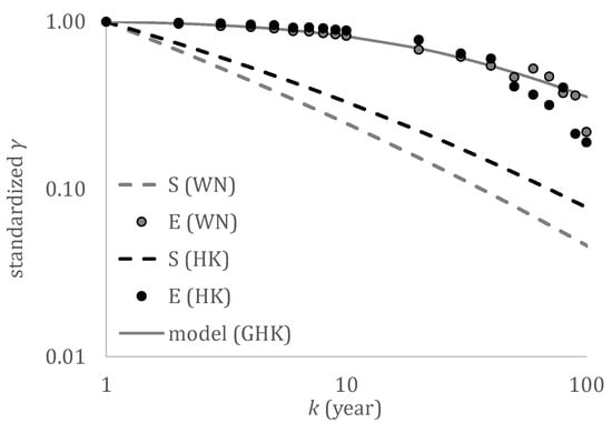
Figure 11.
The standardized climacograms from the stochastic simulation of the streamflow and the produced residential energy for the WN and HK scenarios.
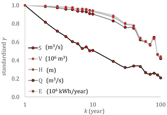
Figure 12.
The standardized climacograms from the stochastic simulation of the streamflow (S), water volume in the reservoir (V), water level in the reservoir (H), output discharge to the turbine (Q) and produced residential energy (E) for the HK scenario.
In summary, in this work, two datasets, i.e., river flow and water volume in the reservoir, have been used to support the successful integration of two methodologies (Bayesian and stochastic) for the calculation of the hydropower energy potential under river flow realization and forecast uncertainties. The applied methodological approach provides the probability of the occurrence of certain reservoir volumes, which are considered significant for hydropower production, while meeting the irrigation needs of the area and the average number of households that can be supplied with electricity from the reservoir and also taking into consideration the effect of the intermediate storage retention due to reservoir’s thresholds. The application of an explicit algorithm for the preservation of the marginal function and dependence structure of the streamflow process, for the simulation of the water balance in the reservoir, for a vast range of scales is considered one of the most important findings of this work. For the marginal structure of the stochastic process, the Hurst and scale parameters are also preserved across scales. These methodologies are unlike those employed in other similar studies, which may preserve the marginal function through data transformation to the the desired marginal distribution, but only implicitly preserving its properties and the autocorrelation structure.
However, there are limitations in the proposed methodology that should be mentioned: for the application of the Bayesian framework, a good fit of a prior probability density function to the river flow process and to the water volume in the reservoir is required. Regarding the stochastic approach, a stationary model for the second-order dependence structure of the river flow timeseries is assumed, whereas for a non-stationary model, an appropriate transformation should apply. Finally, it is found that for a small-sized hydropower plant (as compared to the streamflow magnitude) the curvature of the probability distribution function of the produced energy can be assumed to be negligible as compared to that of the parent distribution of streamflow; it can therefore, be very well approximated by a uniform distribution. Interestingly, the sensitivity analysis performed in the frame of this work shows that the same loss of information occurs also for smaller-sized reservoirs due to the increase of overtopping, while for larger reservoir sizes the information of the distribution tails is preserved and even magnified (see Figure 10 for details).
4. Conclusions
This work presents a methodological framework to assess the hydropower potential of a reservoir following a Bayesian approach and a stochastic analysis of its hydrological potential. The proposed methodology examines, in detail, the steps required to determine the hydropower associated with a specific reservoir water volume. The examined water volumes cover the average water volume in the reservoir, which corresponds to 60% of its maximum capacity, 75% of its maximum capacity and 100% of its maximum capacity. The frequency of occurrence of these volumes is examined assessing hydrological information available from the daily calculated water volume in the reservoir and from the average daily streamflow of the nearby river. The probability distributions of both datasets are determined by fitting established marginal distributions to the river flow process and to the water volume in the reservoir, while the values of the distribution parameters are calculated using a Bayesian approach to determine the associated uncertainty related to the limited reservoir water volume timeseries and to the average calculated daily river flow. The statistical approach produced different results for each dataset (reservoir water volume and streamflow). Although both datasets follow the gamma probability distribution, using the water volume data provides low probabilities (17%) for the reservoir to produce sufficient hydropower considering the base line scenario, while the river flow data provides increased probabilities of up to 44%.
For comparison, a stochastic simulation method used to consider information from both datasets using a Monte Carlo ensemble technique and autocorrelation of the river flow process was also applied. An explicit algorithm was used for the preservation of the marginal function and dependence structure of the streamflow process for the water balance simulation in the reservoir and for a vast range of scales. Specifically, for the marginal function, we preserve the required first moments of the gamma distribution and the long-range dependence (Hurst-Kolmogorov) model (expressed through the climacogram) for the second-order dependence structure of the streamflow process.
The average number of households that can be supplied with electricity from the reservoir, estimated with the two different approaches, are comparable. The results depend though on the different data sources assessed, their different temporal length and the different methodological approach. The Bayesian approach estimates that 366 households can be supplied with electricity for the scenario of average reservoir supply volume; however, with the stochastic simulation it is estimated that between 433 to 454 households can be supplied with hydropower energy. This corresponds to 30% of the population for one of the most populated towns in the area of the reservoir. However, the aim of this work is to provide a decision tool that one can use to assess all the available information and options. It proposes an integrated methodological approach, with several novelties, combining a statistical approach to determine the hydrological potential of the reservoir, a Bayesian analysis to calculate the parameters of the probability distribution for assessing the uncertainty of estimations and the probability of occurrence of specific (significant for hydropower generation) reservoir volumes and also a stochastic approach to account for the effect of the intermediate storage retention due to the reservoir’s thresholds. The probability distribution functions constructed from the stochastic simulation of the streamflow and produced energy show that energy is approximately uniformly distributed for both scenarios (WN and HK) of the stochastic simulation for small- and medium-sized reservoirs, while for larger-sized reservoirs, the information of the streamflow distribution tails is preserved and even magnified. The effects of the intermediate storage retention of the reservoir to the marginal and dependence structures of the parent distribution of inflow and the final energy output are simulated and discussed to highlight the innovation and generalization of the proposed methodology, which can be considered to be an integrated tool for estimating the hydropower potential of any given reservoir. Finally, the results drawn for the specific case study can be of practical use for hydropower generation management in Crete, based on the statistical characteristics of the river that feeds the Faneromeni reservoir.
Author Contributions
Conceptualization, K.S., P.D., E.A.V. and G.A.C.P.; methodology, K.S., P.D., E.A.V. and G.A.C.P.; software, K.S., P.D. and E.A.V.; validation, K.S., P.D. and E.A.V.; formal analysis, K.S. and P.D.; investigation, P.D. and E.A.V.; resources, E.A.V.; data curation, K.S., P.D. and E.A.V.; writing—original draft preparation, K.S. and P.D.; writing—review and editing, K.S., P.D., E.A.V. and G.A.C.P.; visualization, K.S., P.D. and E.A.V.; supervision, K.S.; project administration, E.A.V. and G.A.C.P.; funding acquisition, E.A.V. and G.A.C.P. All authors have read and agreed to the published version of the manuscript.
Funding
This research was funded by the ‘’Prince Albert II foundation’’ under the project “Uncertainty-aware intervention design for Mediterranean aquifer recharge”, http://www.fpa2.org, accessed on 8 January 2022.
Institutional Review Board Statement
Not applicable.
Informed Consent Statement
Not applicable.
Data Availability Statement
Streamflow data for the case study are available at https://data.apdkritis.gov.gr/en (open data), accessed on 8 January 2022.
Conflicts of Interest
The authors declare no conflict of interest. The funders had no role in the design of the study; in the collection, analyses or interpretation of data; in the writing of the manuscript or in the decision to publish the results.
List of Acronyms
| Acronym | Full Name |
| AIC | European Small Hydropower Association |
| E.S.H.A. | European Small Hydropower Association |
| GEV | Generalized Extreme Value |
| HK | Hurst-Kolmogorov |
| P-III | Pearson Type III |
| RMSE | Root Mean Square Error |
| SMA | Symmetric-Moving-Average |
| WN | White Noise |
References
- Mamassis, N.; Efstratiadis, A.; Dimitriadis, P.; Iliopoulou, T.; Ioannidis, R.; Koutsoyiannis, D. Water and energy. In Handbook of Water Resources Management: Discourses, Concepts and Examples; Bogardi, J.J., Tingsanchali, T., Nandalal, K.D.W., Gupta, J., Salamé, L., van Nooijen, R.R.P., Kolechkina, A.G., Kumar, N., Bhaduri, A., Eds.; Springer Nature: Basel, Switzerland, 2021; Chapter 20; pp. 617–655. [Google Scholar] [CrossRef]
- Berga, L. The Role of Hydropower in Climate Change Mitigation and Adaptation: A Review. Engineering 2016, 2, 313–318. [Google Scholar] [CrossRef] [Green Version]
- E.U. Directive (EU) 2018/2001 of the European Parliament and of the Council of 11 December 2018 on the promotion of the use of energy from renewable sources. Off. J. Eur. Union 2018, 5, 82–209. [Google Scholar]
- Holzleitner, M.; Moser, S.; Puschnigg, S. Evaluation of the impact of the new Renewable Energy Directive 2018/2001 on third-party access to district heating networks to enforce the feed-in of industrial waste heat. Util. Policy 2020, 66, 101088. [Google Scholar] [CrossRef]
- Liu, D.; Liu, H.; Wang, X.; Kremere, E. World Small Hydropower Development Report 2019: Case Studies. United Nations Industrial Development Organization; International Center on Small Hydro Power. 2019. Available online: www.smallhydroworld.org (accessed on 8 January 2022).
- Kuriqi, A.; Pinheiro, A.N.; Sordo-Ward, A.; Garrote, L. Influence of hydrologically based environmental flow methods on flow alteration and energy production in a run-of-river hydropower plant. J. Clean. Prod. 2019, 232, 1028–1042. [Google Scholar] [CrossRef]
- Kuriqi, A.; Pinheiro, A.N.; Sordo-Ward, A.; Bejarano, M.D.; Garrote, L. Ecological impacts of run-of-river hydropower plants—Current status and future prospects on the brink of energy transition. Renew. Sustain. Energy Rev. 2021, 142, 110833. [Google Scholar] [CrossRef]
- Special Water Secretariat of Greece. Integrated Management Plans of the Greek Watersheds; Ministry of Environment & Energy: Athens, Greece, 2017.
- Tzanakakis, V.A.; Angelakis, A.N.; Paranychianakis, N.V.; Dialynas, Y.G.; Tchobanoglous, G. Challenges and Opportunities for Sustainable Management of Water Resources in the Island of Crete, Greece. Water 2020, 12, 1538. [Google Scholar] [CrossRef]
- Kusre, B.C.; Baruah, D.C.; Bordoloi, P.K.; Patra, S.C. Assessment of hydropower potential using GIS and hydrological modeling technique in Kopili River basin in Assam (India). ApEn 2010, 87, 298–309. [Google Scholar] [CrossRef]
- Larentis, D.G.; Collischonn, W.; Olivera, F.; Tucci, C.E.M. Gis-based procedures for hydropower potential spotting. Energy 2010, 35, 4237–4243. [Google Scholar] [CrossRef]
- Palomino Cuya, D.G.; Brandimarte, L.; Popescu, I.; Alterach, J.; Peviani, M. A GIS-based assessment of maximum potential hydropower production in La Plata basin under global changes. Renew. Energy 2013, 50, 103–114. [Google Scholar] [CrossRef]
- Tamm, O.; Tamm, T. Verification of a robust method for sizing and siting the small hydropower run-of-river plant potential by using GIS. Renew. Energy 2020, 155, 153–159. [Google Scholar] [CrossRef]
- Wegner, N.; Mercante, E.; de Souza Mendes, I.; Ganascini, D.; Correa, M.M.; Maggi, M.F.; Boas, M.A.V.; Wrublack, S.C.; Siqueira, J.A.C. Hydro energy potential considering environmental variables and water availability in Paraná Hydrographic Basin 3. J. Hydrol. 2020, 580, 124183. [Google Scholar] [CrossRef]
- Gernaat, D.E.H.J.; Bogaart, P.W.; Vuuren, D.P.V.; Biemans, H.; Niessink, R. High-resolution assessment of global technical and economic hydropower potential. Nat. Energy 2017, 2, 821–828. [Google Scholar] [CrossRef]
- Hatamkhani, A.; Moridi, A.; Yazdi, J. Simulation-Optimization models for multi-reservoir hydropower systems design at watershed scale. Renew. Energy 2020, 149, 253–263. [Google Scholar] [CrossRef]
- Bocchiola, D.; Manara, M.; Mereu, R. Hydropower Potential of Run of River Schemes in the Himalayas under Climate Change: A Case Study in the Dudh Koshi Basin of Nepal. Water 2020, 12, 2625. [Google Scholar] [CrossRef]
- Casale, F.; Bombelli, G.M.; Monti, R.; Bocchiola, D. Hydropower potential in the Kabul River under climate change scenarios in the XXI century. Theor. Appl. Climatol. 2020, 139, 1415–1434. [Google Scholar] [CrossRef]
- Liu, X.; Tang, Q.; Voisin, N.; Cui, H. Projected impacts of climate change on hydropower potential in China. Hydrol. Earth Syst. Sci. 2016, 20, 3343–3359. [Google Scholar] [CrossRef] [Green Version]
- Wang, H.; Xiao, W.; Wang, Y.; Zhao, Y.; Lu, F.; Yang, M.; Hou, B.; Yang, H. Assessment of the impact of climate change on hydropower potential in the Nanliujiang River basin of China. Energy 2019, 167, 950–959. [Google Scholar] [CrossRef]
- Varouchakis, E.A.; Palogos, I.; Karatzas, G.P. Application of Bayesian and cost benefit risk analysis in water resources management. J. Hydrol. 2016, 534, 390–396. [Google Scholar] [CrossRef]
- Varouchakis, E.A.; Yetilmezsoy, K.; Karatzas, G.P. A decision-making framework for sustainable management of groundwater resources under uncertainty: Combination of Bayesian risk approach and statistical tools. Water Policy 2019, 21, 602–622. [Google Scholar] [CrossRef]
- Stickler, C.M.; Coe, M.T.; Costa, M.H.; Nepstad, D.C.; McGrath, D.G.; Dias, L.C.; Rodrigues, H.O.; Soares-Filho, B.S. Dependence of hydropower energy generation on forests in the Amazon Basin at local and regional scales. Proc. Natl. Acad. Sci. USA 2013, 110, 9601e9606. [Google Scholar] [CrossRef] [Green Version]
- Chen, L.; Huang, K.; Zhou, J.; Duan, H.F.; Zhang, J.; Wang, D.; Qiu, H. Multiple-risk assessment of water supply, hydropower, and environment nexus in the water resources system. J. Clean. Prod. 2020, 268, 122057. [Google Scholar] [CrossRef]
- Liao, S.; Liu, B.; Cheng, C.; Li, Z.; Wu, X. Long-term generation scheduling of hydropower system using multicore parallelization of particle swarm optimization water resources management an international. Water Resour. Manag. 2017, 31, 2791–2807. [Google Scholar] [CrossRef]
- Li, L.; Liu, P.; Rheinheimer, D.E.; Deng, C.; Zhou, Y. Identifying explicit formulation of operating rules for multi-reservoir systems using genetic programming. Water Resour. Manag. 2014, 28, 1545–1565. [Google Scholar] [CrossRef]
- Shi, Y.; Yong, P.; Wei, X.U. Optimal operation model of cascade reservoirs based on grey discrete differential dynamic programming. J. Hydroelectr. Eng. 2016, 35, 35–44. [Google Scholar]
- Mujumdar, P.P.; Nirmala, B. A Bayesian Stochastic optimization model for a multi-reservoir hydropower system. Water Resour. Manag. 2007, 21, 1465–1485. [Google Scholar] [CrossRef] [Green Version]
- Celeste, A.B.; Billib, M. Evaluation of stochastic reservoir operation optimization models. Adv. Water Resour. 2009, 32, 1429–1443. [Google Scholar] [CrossRef]
- Xu, W.; Zhang, C.; Peng, Y.; Fu, G.; Zhou, H. A two stage Bayesian stochastic optimization model for cascaded hydropower systems considering varying uncertainty of flow forecasts. Water Resour. Res. 2014, 50, 9267–9286. [Google Scholar] [CrossRef]
- Tan, Q.; Fang, G.; Wen, X.; Lei, X.-H.; Wang, X.; Wang, C.; Ji, Y. Bayesian Stochastic Dynamic Programming for Hydropower Generation Operation Based on Copula Functions. Water Resour Manag. 2020, 34, 1589–1607. [Google Scholar] [CrossRef]
- Lei, X.H.; Tan, Q.F.; Wang, X.; Wang, H.; Wen, X.; Wang, C.; Zhang, J.W. Stochastic optimal operation of reservoirs based on copula functions. J. Hydrol. 2017, 557, 265–275. [Google Scholar] [CrossRef]
- Hoeting, J.A.; Madigan, D.; Raftery, A.E.; Volinsky, C.T. Bayesian model averaging: A tutorial. Stat. Sci. 1999, 14, 382–417. [Google Scholar]
- Zhang, J.; Liu, P.; Wang, H.; Lei, X.; Zhou, Y. A Bayesian model averaging method for the derivation of reservoir operating rules. J. Hydrol. 2015, 528, 276–285. [Google Scholar] [CrossRef]
- Xu, W.; Zhao, J.; Zhao, T.; Wang, Z. Adaptive reservoir operation model incorporating nonstationary inflow prediction. J. Water Res. Plan. Man. 2014, 141, 04014099. [Google Scholar] [CrossRef]
- Yang, G.; Zaitchik, B.; Badr, H.; Block, P. A Bayesian adaptive reservoir operation framework incorporating streamflow non-stationarity. J. Hydrol. 2021, 594, 125959. [Google Scholar] [CrossRef]
- Koutsoyiannis, D. HESS Opinions "A random walk on water". Hydrol. Earth Syst. Sci. 2010, 14, 585–601. [Google Scholar] [CrossRef] [Green Version]
- Dimitriadis, P.; Koutsoyiannis, D. Climacogram versus autocovariance and power spectrum in stochastic modelling for Markovian and Hurst–Kolmogorov processes. Stoch. Environ. Res. Risk A 2015, 29, 1649–1669. [Google Scholar] [CrossRef]
- Zhang, X.; Wang, X.; Wang, X.; Chen, H. Energy uncertainty risk management of hydropower generators. In Proceedings of the IEEE/PES Transmission & Distribution Conference & Exposition: Asia and Pacific, Dalian, China, 18 August 2005; pp. 1–6. [Google Scholar] [CrossRef]
- Basso, S.; Botter, G. Streamflow variability and optimal capacity of run-of-river hydropower plants. Water Resour. Res. 2012, 48, W10527. [Google Scholar] [CrossRef]
- Kocaman, A.S.; Modi, V. Value of pumped hydro storage in a hybrid energy generation and allocation system. Appl. Energy 2016, 205, 1202–1215. [Google Scholar] [CrossRef] [Green Version]
- Li, H.; Liu, P.; Guo, S.; Ming, B.; Cheng, L.; Yang, Z. Long-term complementary operation of a large-scale hydro-photovoltaic hybrid power plant using explicit stochastic optimization. Appl. Energy 2019, 238, 863–875. [Google Scholar] [CrossRef]
- Labadie, J.W.; Fontane, D.G.; Tabios III, G.Q.; Chou, N.F. Stochastic Analysis of Dependable Hydropower Capacity. J. Water Resour. Plan. Manag. 1987, 113, 422–437. [Google Scholar] [CrossRef]
- Ouarda, T.B.M.; Labadie, J.W.; Fontane, D.G. Indexed sequential hydrologic modeling for hydropower capacity estimation. J. Am. Water Resour. Assoc. 1997, 33, 1337–1349. [Google Scholar] [CrossRef]
- Zhao, T.; Cai, X.; Yang, D. Effect of streamflow forecast uncertainty on real-time reservoir operation. Adv. Water Resour. 2011, 34, 495–504. [Google Scholar] [CrossRef]
- Côté, P.; Leconte, R. Comparison of Stochastic Optimization Algorithms for Hydropower Reservoir Operation with Ensemble Streamflow Prediction. J. Water Resour. Plan. Manag. 2016, 142, 04015046. [Google Scholar] [CrossRef]
- Ávila, L.R.; Mine, M.R.M.; Kaviski, E.; Detzel, D.H.M.; Fill, H.D.; Bessa, M.R.; Pereira, G.A.A. Complementarity modeling of monthly streamflow and wind speed regimes based on a copula-entropy approach: A Brazilian case study. Appl. Energy 2020, 259, 114127. [Google Scholar] [CrossRef]
- Efstratiadis, A.; Tsoukalas, I.; Koutsoyiannis, D. Generalized storage-reliability-yield framework for hydroelectric reservoirs. Hydrol. Sci. J. 2021, 66, 580–599. [Google Scholar] [CrossRef]
- Koutsoyiannis, D. Generic and parsimonious stochastic modelling for hydrology and beyond. Hydrolog. Sci. J. 2016, 61, 225–244. [Google Scholar] [CrossRef]
- Dimitriadis, P.; Koutsoyiannis, D. Stochastic synthesis approximating any process dependence and distribution. Stoch. Environ. Res. Risk A 2018, 32, 1493–1515. [Google Scholar] [CrossRef]
- Koutsoyiannis, D.; Dimitriadis, P. Towards generic simulation for demanding stochastic processes. Science 2021, 3, 34. [Google Scholar] [CrossRef]
- Varouchakis, E.A.; Theodoridou, P.G.; Karatzas, G.P. Spatiotemporal geostatistical modeling of groundwater levels under a Bayesian framework using means of physical background. J. Hydrol. 2019, 575, 487–498. [Google Scholar] [CrossRef]
- Tapoglou, E.; Vozinaki, A.E.; Tsanis, I. Climate Change Impact on the Frequency of Hydrometeorological Extremes in the Island of Crete. Water 2019, 11, 587. [Google Scholar] [CrossRef] [Green Version]
- Vozinaki, A.E.K.; Tapoglou, E.; Tsanis, I.K. Hydrometeorological impact of climate change in two Mediterranean basins. Int. J. River Basin Manag. 2018, 16, 245–257. [Google Scholar] [CrossRef]
- Decentralized Administration of Crete, 2020. Water Resources Portal. Region of Crete, Directorate of Water, Heraklion. Available online: http://www.apdkritis.gov.gr/en/group/hydrology (accessed on 8 January 2022).
- European Small Hydropower Association. Guide on How to Develop a Small Hydropower Plant; European Small Hydropower Association: Brussels, Belgium, 2004. [Google Scholar]
- Forbes, C.; Evans, M.; Hastings, N.; Peacock, B. Statistical Distributions; John Wiley & Sons: Hoboken, NJ, USA, 2011. [Google Scholar]
- Akaike, H. A new look at the statistical model identification. ITAC 1974, 19, 716–723. [Google Scholar] [CrossRef]
- Bolstad, W.M.; Curran, J.M. Introduction to Bayesian Statistics; John Wiley & Sons: Hoboken, NJ, USA, 2016. [Google Scholar]
- Hurst, H.E. Long Term Storage Capacity of Reservoirs. Trans. Am. Soc. Civ. Eng. 1951, 116, 776–808. [Google Scholar] [CrossRef]
- Koutsoyiannis, D. A generalized mathematical framework for stochastic simulation and forecast of hydrologic time series. Water Resour. Res. 2000, 36, 1519–1533. [Google Scholar] [CrossRef] [Green Version]
- Finley, A.O.; Banerjee, S.; Gelfand, A.E. spBayes for Large Univariate and Multivariate Point-Referenced Spatio-Temporal Data Models. J. Stat. Softw. 2015, 63, 1–28. [Google Scholar] [CrossRef]
- Dimitriadis, P.; Koutsoyiannis, D.; Iliopoulou, T.; Papanicolaou, P. A Global-Scale Investigation of Stochastic Similarities in Marginal Distribution and Dependence Structure of Key Hydrological-Cycle Processes. Hydrology 2021, 8, 59. [Google Scholar] [CrossRef]
- Koutsoyiannis, D.; Dimitriadis, P.; Lombardo, F.; Stevens, S. From fractals to stochastics: Seeking theoretical consistency in analysis of geophysical data. In Advances in Nonlinear Geosciences; Tsonis, A.A., Ed.; Springer: Berlin/Heidelberg, Germany, 2018; pp. 237–278. [Google Scholar] [CrossRef]
Publisher’s Note: MDPI stays neutral with regard to jurisdictional claims in published maps and institutional affiliations. |
© 2022 by the authors. Licensee MDPI, Basel, Switzerland. This article is an open access article distributed under the terms and conditions of the Creative Commons Attribution (CC BY) license (https://creativecommons.org/licenses/by/4.0/).