Abstract
In the context of an eco-responsible production and distribution of electrical energy at the local scale of an urban territory, we consider a smart grid as a system interconnecting different prosumers, which all retain their decision-making autonomy and defend their own interests in a comprehensive system where the rules, accepted by all, encourage virtuous behavior. In this paper, we present and analyze a model and a management method for smart grids that is shared between different kinds of independent actors, who respect their own interests, and that encourages each actor to behavior that allows, as much as possible, an energy independence of the smart grid from external energy suppliers. We consider here a game theory model, in which each actor of the smart grid is a player, and we investigate distributed machine-learning algorithms to allow decision-making, thus, leading the game to converge to stable situations, in particular to a Nash equilibrium. We propose a Linear Reward Inaction algorithm that achieves Nash equilibria most of the time, both for a single time slot and across time, allowing the smart grid to maximize its energy independence from external energy suppliers.
1. Introduction
The eco-responsible production and distribution of electrical energy at the local scale of an urban territory (a district—an activity zone for example) is today an environmental and economic key objective in the development or the planning of such territories [1,2]. Indeed, the trend of governance of urban territories, which often wish to keep or gradually regain control of their infrastructure networks (water, energy, mobility, and waste), is to deploy, in the energy sector, smart grids interconnecting private and public actors (companies, administrations, and residential buildings, for example) [1,3], each potentially having a green electricity production and storage capacity; they act as prosumer actors [4,5].
In this context of a smart grid interconnecting different prosumers, two operating paradigms can be considered. On the one hand, a totally collaborative operating mode in which each actor leaves its autonomy of decision to a centralized system, which acts towards global optimization and distributes the final costs to each actor (for example through a mechanism using Shapley values [6]). On the other hand, a more selfish mode of operation in which each actor retains its decision-making autonomy and defends its own interests in a comprehensive system with rules, which are accepted by all, that encourage virtuous behavior. It is this second paradigm that we consider here. Indeed, as it is unlikely that an actor, in particular an industrial actor, would agree to leave, to an independent operator, the control of the use of its own means of production and storage of energy, this second paradigm seems more realistic.
To be accepted by all, a strategy must be able to guarantee to each actor that it will be more advantageous than a situation of pure selfishness, which is the objective of this article. Thus, our objective is to propose and analyze a model and a management method for a smart grid that is shared between different independent actors, who respect their own interests, and that encourages each to a behavior allowing as much as possible an energy independence of the smart grid from external energy suppliers. This respect for the interests and independence of each actor naturally leads us to consider not the search for a global optimum between the actors, but more of a virtuous balance of their politics that is beneficial to all.
This is why we consider here a game theory model, in which each actor of the smart grid is a player, and we investigate distributed machine-learning algorithms to allow decision-making, thus, leading the game to converge to a stable situation, in particular Nash equilibria if they exist (see [7] for a definition). From a control systems engineering perspective, reinforcement learning (RL) can be considered a closed-loop process [8,9], which means that, at each learning step, the control system is feedback-regulated (as opposed to open-loop controllers, which do not consider process output and only calculate commands using internal or external parameters).
In our context of using RL, the feedback resides in the reward values of each step that are used to calculate new probabilities of actions vis-à-vis of the smart grid, actions to be selected by each prosumer at the next step. The closed-loop process is therefore considered here at the level of granularity of the set of prosumers and their decisions across time, and not at that of the management of electrical devices for which closed-loop processes are also proposed [10,11]. At the level of granularity we consider here, we make no fixed assumptions about the type of control used for real-time management of electrical devices, closed-loop or open-loop.
Some early works (as of the 2010s) focused mainly on the use of game theory for energy supply to end consumers [12,13,14]. As renewable local energy production capabilities became increasingly available, some work focused on considering those energy production capabilities in smart grid models, leading to including prosumers (i.e., producers/consumers) in those models. In [15], the authors proposed a game theory approach to model the interactions among prosumers and distribution system operators for the control of electricity flows in real-time.
The authors in [16] proposed a game theory energy management based on the Stackelberg leadership model system, which seeks for social optimality when each energy consumer focuses only on its own energy efficiency; the existence of a Nash equilibrium for any instance of the game model that is proposed in the paper was proven (we will see that this is not the case for the game model that we consider, see Lemma 1), and an optimal distributed deterministic algorithm is proposed that reaches this equilibrium.
Some other works seek to propose pricing policies for energy suppliers, considering various optimization objectives. In [17], the authors considered a smart power infrastructure where several subscribers share a common energy source, and proposed a distributed algorithm that automatically manages the interactions among subscribers and the energy provider. The authors in [18] presented an equilibrium Selection Multi-Agent Reinforcement Learning for consumer energy scheduling of a residential microgrid, based on private negotiation between each consumer and the energy provider, and the work of [19] include reliability parameters and energy fluctuations and propose a Deep Reinforcement Learning algorithm based on Q-Learning and Deep Neural Networks to determine a pricing policy for a power supplier that balances those two parameters.
The authors in [20] also proposed a Vickrey–Clarke–Groves (VCG)-based auction mechanism aiming to maximize the aggregate utility functions of all users minus the total energy cost. In [21], the authors proposed a game theory approach for selecting the best power subscription when several power suppliers are available, based on a two-stage process.
Taking into account the availability of several power suppliers leads to various Demand Response Management (DRM) problems. The results of [22] focused on the real-time interactions among multiple utility companies and multiple users, and they proposed a distributed real-time demand response algorithm to determine each user’s demand and each utility company’s supply simultaneously.
The contributions of [23] also focused on DRM but solved electricity pricing questions using a reinforcement learning-based decision system. The goal in this approach is to minimize the electricity payment and consumption dissatisfaction for end users. Some works focused on more distributed models with autonomy goals. The authors in [24] proposed a coalition game between a number of micro-grids (energy producers) that are each servicing a group of consumers (or an area), and [25] also considered autonomy goals for a distributed set of micro-grids without support from a traditional centralized grid and proposed a distributed algorithm based on a cooperative game theory approach. In [26], a Q-learning method was proposed in a multi-agent model where each consumer (and more particularly each smart meter) adapts its consumption and the control of its electrical equipment to the state of the grid and to the prices of electricity.
This synthetic review on related works leads to one observation: very few works focused on a general smart grid model, in which consumers may or may not have power production capabilities and power storage facilities, and considered learning approaches. To our knowledge, only [27] proposed a multi-agent reinforcement-learning approach to controlling a smart grid composed of production resources, battery storage, electricity self-supply, and short-term market trading. Event though the proposed algorithm offers a significantly high computation speed, it has local optima issues that cause it to be out-performed by the use of a simulated annealing in terms of energy costs.
We propose here a new game theory model for a smart grid interconnecting different prosumers. This game theory model is based on the proposal of a virtual economic model between the players, which has an impact on the amount of energy that the smart grid has to buy from an external supplier. In a discrete time context, in order to allow the smart grids to obtain an operation that is as little dependent as possible on such an external energy supplier, while respecting the constraints and interests of each actor, we develop and experiment on different scenarios a distributed reinforcement-learning approach aimed at achieving each time period of use of the smart grid. Indeed, the objective here is to propose a decision algorithm that, on the one hand, respects the choices and the interests of each actor and, on the other hand, does not require a large data history. This is why we decided to use a reinforcement-learning approach distributed between the actors and not a centralized supervised or unsupervised learning approach (see for example [28,29]).
The remainder of the article is structured as follows: first, in Section 2—Materials and Methods, we define the architecture of the considered system, i.e., the various actors, their interactions, and their actions. This section then specifies the game model considered, as well as the internal economic model that this game implements. In Section 2.2—Distributed Reinforcement Learning for the Game in Each Period, the distributed reinforcement-learning model that will be used for the simulations is defined. In Section 3—Results, the performance evaluation of the proposed reinforcement learning executed at each period is analyzed. The behavior of this approach over a series of periods is then analyzed in Section 3.2—Multi-Period Simulation.
2. Materials and Methods
2.1. Smart Grid Model
In this section, we define the actors of the smart grid, their interactions, the associated multi-agent game model, and the virtual economic model that governs it. The main parameters and notations of the proposed model are given in Table 1—a list of the main notations defining the components of the smart grid model and their interactions.

Table 1.
List of main notations defining the components of the smart grid model and their interactions.
2.1.1. Smart Grid Actors Model
Our model assumes that each day is divided into homogeneous consecutive periods of a few hours. We make two assumptions here. First, that the consumption and production values of each actor in each period can be considered as a fixed value. Secondly, that it is possible at each period and for each actor to sufficiently predict precisely these consumption and production values for the following period. In [30], it is shown that such a model is realistic considering half-day periods, but it is important to note that our model is independent of the choice of periods—the execution of the method requires a short time in each one.
In this discrete time context, each energy indicator of each actor can be considered as a fixed value in each period. For each period, the system representing the smart grid is considered here as a multi-agent system. Let be the set of N actors connected by the smart grid (SG), each actor being potentially able to produce electricity, in particular with renewable energies, and to store it. Each actor’s production and storage capacities are limited. Production varies over periods.
Each actor , with , at each period t is characterized by
- is the production of electricity by the actor during the period.
- is the electricity consumption of the actor during the period.
- is the quantity of electricity stored by the actor at the beginning of the period. We denote by the maximal storage capacity, and we define the residual capacity of battery storage , i.e., the maximum quantity of energy that the actor can store during the period. Note that, during a period, an actor cannot both use and provide storage.
As has been done in different game models applied to Smart Grids [31,32,33], at the level of granularity corresponding to the model we use here, where a single prosumer can be a micro-grid, we consider at a first approach that the values of consumption and production are inelastic in each period, which thus makes it possible to assess the relevance of algorithmic game theory to arbitrate the choices of the various independent actors. This relevance established, taking into account inelastic data at a finer granularity could then be considered [34,35,36], in game models that are likely to be more complex to handle.
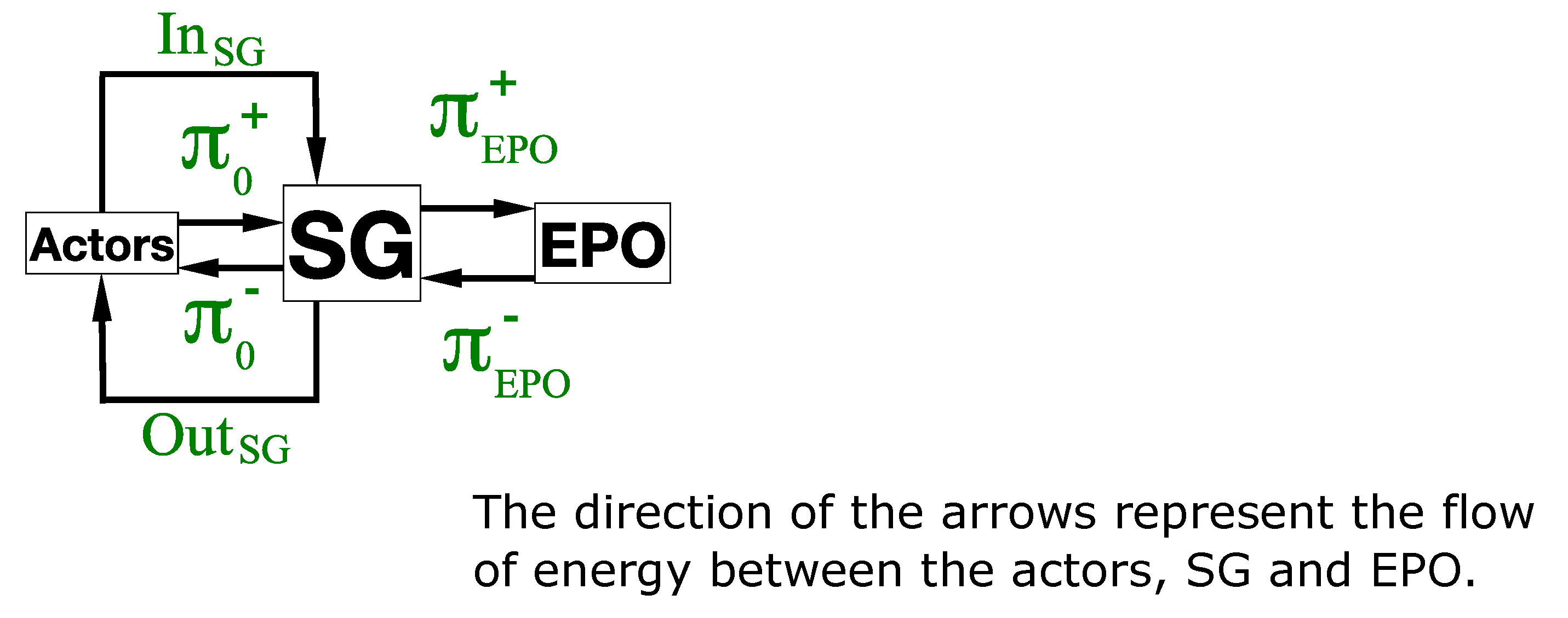
The smart grid is also connected to an external energy production operator (EPO), who can supply it with electricity if necessary and to which the smart grid can sell unused electricity produced by the actors. Note that the actors do not directly interact with this EPO.
Thus, the smart grid itself can be considered as an energy container connecting all the actors ; each actor at each period t provides a quantity of electricity to SG and uses a quantity of electricity from SG (note that and cannot be both greater than 0). We denote and . Then, if , the energy production operator EPO provides a quantity of energy to SG from a given linear increasing cost function (see Section 3.1—Learning Performance Analysis); else if , SG sells a quantity of energy from a given linear increasing benefit function . Definitions of and are inputs of the model.
2.1.2. Action Modes of Each Actor
At each period t, each actor chooses one of four possible modes of action . Modes and mean that the actor requires energy from SG for its consumption, i.e., and its production is not sufficient to cover its consumption (the two modes differ on whether the actor uses its storage or not, as detailed below). Mode means that the actor decides to be independent of SG (i.e., ). Finally, mode means that the actor chooses to provide energy to SG (i.e., , and it is autonomous for its own consumption). The conditions to choose one mode in respect the following rules considering three disjoint states for an actor depending only on .
- State Deficit: . In this state, actor needs energy from SG for its consumption, then ; it can also choose to use its storage or not. Thus, in this state, the chosen mode can be , in which case and thus , or , in which case and thus .
- State Self: and . In this state, two modes can be chosen by . First, , where : the actor does not use its storage, . Secondly , where and . In both cases, .
- State Surplus: . Two modes can be chosen by . First, , where : the actor provides all its overall produced energy to SG and remains the same. Secondly, in which and : the actor favors the storage of its remaining produced energy. In both cases, .
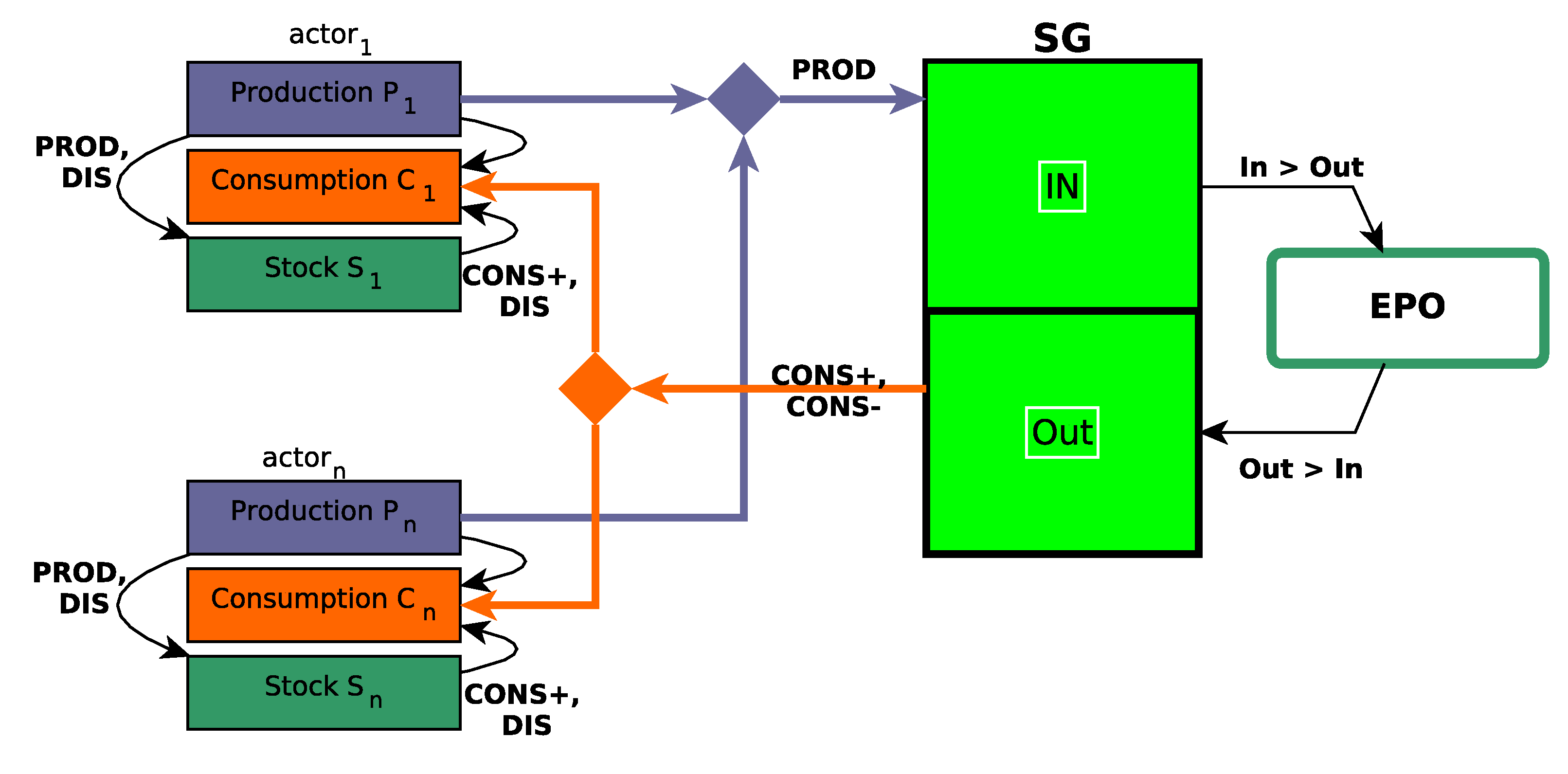
The logical architecture of the system thus proposed is synthesized in Figure 1.

Figure 1.
Logical architecture of the whole considered system.
Thus, in State Deficit, each actor can choose at each period t its mode in . In State Self, an actor can choose its mode in . Finally, in State Surplus, an actor can choose its mode in . Thus, in any case, an actor has always two possible strategies.
These modes ensure that the production of the actor is intended primarily for its consumption, and the stored energy of is never imported from SG but is only filled by its own production. In fact, each actor consumes the total amount of production (and eventually its current storage) before importing electricity from SG. The choice of actors therefore only concerns the policy of supply or use of the stock.
Let us now define two parameters and such as and . Note that is an upper bound of the energy quantity bought by SG to EPO at period t and that is an upper bound of the energy quantity sold by SG to EPO at period t. We then also define and (in fact, we consider that way a kind of linearization of functions and ).
We define two other parameters, and . First, is a cost each actor has to pay for one unit of energy provided to it by SG. Secondly, is a benefit each actor makes for one unit of energy sold to SG (see Figure 2 Unitary prices in the model used for learning process). This guaranties that, for any , we have . These two parameters are not input data but rather parameters of the virtual economic internal model of SG, needed for its management; the way to choose values for and will be discussed in Section 2.1.2—Action Modes of Each Actor.
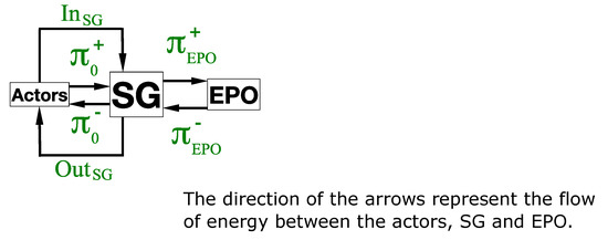
Figure 2.
Unitary prices in the model used for the learning process.
Then, the internal cost and benefits of each actor defined in the model depend on the value of , , and . We first define a unitary cost Equation (1) and a unitary benefit Equation (2) of a unit of energy in SG as follows:
These definitions are based on choices relating to the proposed model. If , then we consider that each actor in state Deficit, or in state Self with mode , receives the same percentage of energy supplied globally by EPO. This percentage is then reflected on the unit cost . On the contrary, if , then we consider that each actor in state Surplus sells the same percentage of energy to EPO, which is reflected in the unit benefit .
To finally define the cost and benefit functions of each actor at each period t, we consider a given parameter which indicates the importance given by each actor of storing energy for the next period, with . Each actor at each period t knows and . The way to determine the value of each will be considered in Section 2.2.1—Learning strategies.
The (virtual) whole cost of at period t is and its whole benefit is , with the additional or preserved stock indicating the amount of energy stored or preserved by the actor for the next period defined as follows:
- If then .
- If then .
- If then in State Self and in State Surplus.
- If then .
Thus, we denote by the value of actor at period t. We also consider and being respectively the internal benefit and cost of actor for all the periods in the virtual economic model we propose inside SG.
2.1.3. Game Model
From the definitions of the previous section, we consider, in each period, a simultaneous game model [7], called SGGame, in which players are the actors and where the set of strategies of player is if is in State Deficit, if is in State Self and if is in State Surplus.
Given a strategy profile , with a strategy for each player , we define the utility of player by . Note that, since and can be different from the other and different from and , this game called SGGame is not a zero-sum game [7].
Let us recall that a Nash equilibrium is a strategic profile in which the unilateral modification of the strategy of any actor degrades its utility [7] (thus, no actor has any interest in changing its strategy alone). As shown in Section 3.1—Learning performance analysis, non-trivial instances of the game admit pure Nash equilibria. The following result proves that this is not always the case.
Lemma 1.
SGGame does not admit a pure Nash equilibrium for all instances.
Proof.
We consider an instance of SGGame with two players in State Deficit and in State Surplus, with
- and .
- and .
- and .
Note that these values of and are compatible with what will be defined in Section 3.1. □
Then, we can have four possible strategy profiles depending on strategies for and for , and the utilities are given in Table 2.
Table 2.
Utilities for each possible strategy profile.
Note that this lemma is a consequence of the differences between the values of , , and .
As we have seen, we consider the time of the smart grid as a sequence of T homogeneous periods of the same duration. Each actor is in a chosen mode in for each period (modes determined by running the game considering the state of each actor). Thus, the system can be seen as a non-stationary repeated game. It is non-stationary because the values of and of at each step do not depend (only) on the strategies chosen during the previous steps. Moreover, since the choice of strategies for each period, apart from the value of the stock of each actor, does not depend on the strategies chosen during previous periods, we cannot here directly consider concepts of the theory of repeated games [37].
2.1.4. A Pricing Model for a Smart Grid
As we have seen, the model proposed here is an internal and virtual economic model between SG actors to be used as a cost allocation key for the real payment of electricity purchased from EPO by all the actors.
The objective is thus here to propose a mechanism to compute a unit price of purchase and sale of electricity to each actor for the whole periods, prices whose modifications compared to the real price of EPO will depend on the choice of all the players during all the periods. Thus, there is no real financial exchange here between the actors, or between the actors and SG (again, the internal economic model is virtual). This model will be the basis of how to fix and for each period t.
For each actor , let us denote and . It is clear that , i.e., all of what is produced in SG by , is not sold to EPO, and that , ie all of what is consumed from SG by , is not purchased from EPO. Thus, we propose here that the real cost has to pay for the T periods is and the real benefit of is with
and
Then, the real economic balance of actor for all the periods is . Note that the sum of the actors profits is equal to the benefit of SG on EPO, and that the sum of the actors costs is equal to the overall price paid by SG to EPO.
It will therefore be a question of determining at each period t the values of and , which offers the best compromise between the value and that are implied by and . Since the purpose of each actor of the game in each period t is to make the best decision regarding the whole proposed economic model, we use definitions of and to set values of and at each period t as follows: and . Note that more is close to , with , more the fact that an actor in state Surplus provides electricity to the smart grid is required, which is why has to be close from in such cases.
We consider that initially and . As said in Section 2.1.3—Game model, due to the energy market rules, since and , and are not necessarily equal, each period t does not consist in a zero-sum game and thus some situations could occur in which all actors utilities are positive (or negative).
2.2. Distributed Reinforcement Learning for the Game in Each Period
Based on the models given above, we propose here a distributed reinforcement-learning approach which objective is to make it possible to converge towards situations that are stable, i.e., in which a choice of strategy for each actor having a significant impact on the state of the smart grid is on one hand clearly established with a high probability and on the other hand optimized from the point of view of the cost for all the actors. In particular, in the game model we are introducing, we observe experimentally on the instances we generate that Nash equilibria (see [7] for a definition) are, when they exist, such stable situations.
2.2.1. Learning Strategies
We consider at each period t the game defined in Section 2.1.3—Game model. Note that in a distributed reinforcement learning context, if some actors in state Deficit are such that , then any strategy in lets them in a same situation. Thus, in the following, we do not consider such an actor as a player, even if we consider its impact in the computation of the utilities for the other (real) players.
The objective of the learning strategy is to attempt to reach a good stable situation, or even a Nash equilibrium, at each period, considering the benefit function defined in Section 2.1.3—Game model. The utility function we use in this learning strategy is based on a benefit/cost parameter for each player at each learning step k, depending on the storage parameter computed as follows:
Given a period , whatever is the state of the actor , the two modes this actor can choose to have different impact on the storage quantity at the end of the period. Let us denote, by , the maximum of these two values and the minimum one.
- State Deficit: , considering and , considering .
- State Self: , considering , and , considering .
- State Surplus: , considering , and , considering .
One can check that . Consider now the probability
is the ideal quantity of energy that actor should have in stock for period . Let be a random variable where the value is 1 with probability , else . Then, we set with if is in State Deficit or Self, else if is in state Surplus.
We can now define the utility function we propose to use.
First, considering Section 2.1.3—Game model, we compute the following bounds of and (see end of Section 2.1.2—Action modes of each actor for definitions):
Then, we can conclude that
Note that (resp. ) is computed by considering that each actor in State Surplus is in mode (resp. ). The value of (resp ) is computed by considering that each actor in State Deficit is in mode and that each actor in State Self is in mode ; finally, is computed by considering that each actor in State Deficit or Self is in mode . The game benefit of a player at step k is defined by . and . Note also that is an upper bound of the cost actor could have to pay.
We denote by and the minimum and maximum benefits obtained by the player during learning step from 1 to k. Then, the utility of during step k of the learning process of period t is equal to .
2.2.2. Learning Process
Based on the strategy given above, we consider here a distributed Linear Reward Inaction (LRI) reinforcement learning process (see [38]).
Each actor is characterized by two possible strategies and . Let us denote by the probability to choose strategy at step k and by the probability to choose strategy at step k. Let the chosen strategy, with . Then,
with a learning parameter called slowdown factor. The probability of the other strategy at step is of course .
3. Results
We present in this section several experiments and performance evaluations of the LRI reinforcement learning process presented above.
The performance evaluation of the approach proposed here is based on a set of data generated as indicated in Section 3.1 and Section 3.2, for about twenty actors. The purpose of this generation is on the one hand to represent realistic situations in terms of heterogeneity of actors’ behavior (production and consumption) and on the other hand to be sufficiently complex in terms of learning process to evaluate the performances of the method (in particular on the existence or not of pure Nash equilibria).
We start by studying the performances of the learning process during only one period. We then extend our simulations to cases in which the learning process runs on several successive periods.
3.1. Learning Performance Analysis
We first study here the performance of the learning strategies on only one period t. To do this, considered data are generated as follows: Experiments are done on 50 independent period instances. The values of and of actor is computed by:
- If , then and is uniformly chosen in ; we consider .
- If , then with probability , we set and uniformly chosen in and we consider . Else, we set and uniformly chosen in , and we consider
- If , then and uniformly chosen in , and we consider .
We consider 15 actors in state Deficit, 10 actors in State Surplus and 10 actors in State Self. For each actor , we set . Finally, we consider , , and . The value of each value is computed as defined in Section 2.2.1—Learning strategies, considering that .
The 50 instances generated correspond each to a difficult context for SG, i.e., in which SG is highly dependent on EPO. For each instance, we consider the average value of over the 50 tested instances (see the end of Section 2.1.2—Action modes of each actor for definition of ).
We compare the performances of the reinforcement learning process (RL) described above, with parameter , with a total exploration method (TEM) to find a strategy profile maximizing (note that such method seems to be impracticable in real situations because of computation time when N is not small), considering also the maximum value of over all Nash equilibria, if at least one exists. The learning algorithm RL is stopped when, for each actor and before 50,000 learning steps (maximum number of learning steps), the highest probability of the strategic of each actor is greater than or equal to ; we refer to this situation as stabilization, and it is the strategy with such maximum probability that is chosen for each actor. Otherwise, the learning process is stopped after 50,000 steps. The chosen strategic profile is made up for each player in the strategy with the highest probability.
Experiments show first that the set of generated instances each admits a non-empty set of Nash equilibria, which are all equivalent, i.e., where only variations concern the strategies of certain actors in deficit mode, variations that do not change the utility of any player. These Nash equilibria therefore all have the same value. This value is minimum on all possible strategic profiles, and only these balances reach this value, as indicated by the execution of TEM. The ratio between the best and the worst value of for a profile is on average among all the instances, which shows the variability of the set of strategic profiles for each instance in terms of performance.
The learning method stabilizes for 12 instances over 36, with an average of 18,000 learning steps for those 12 instances. Whether the method has stabilized or not, the strategic profile provided is in all cases a Nash equilibrium. We can conclude that on this set of instances, RL requires a relatively small number of steps to determine the Nash equilibrium, whether it stabilizes or not. Moreover, the evolution of the strategy probabilities during the learning process reveals two types of well-discriminated instances. By definition, actors and instances for which learning stabilizers have a maximum probability greater than . For each of the other instances, the mean value of the maximum probability is globally comprised between and .
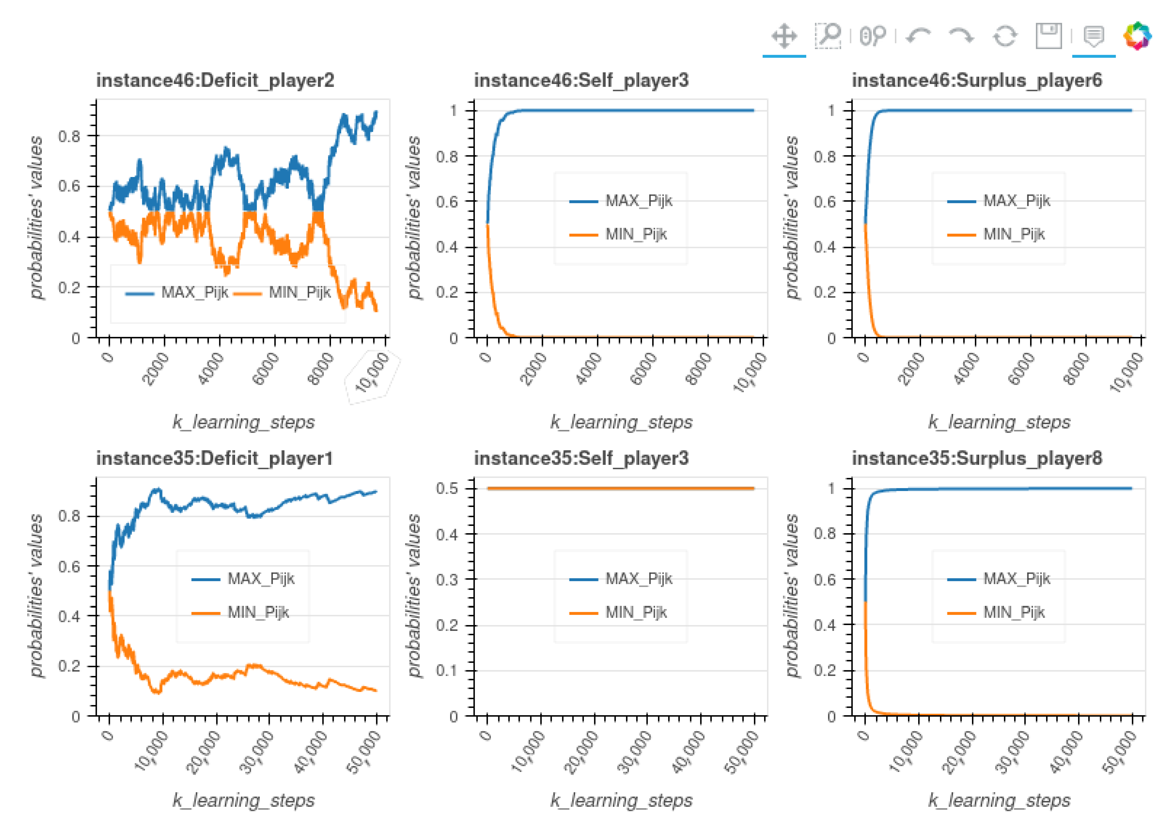
Figure 3 Examples of stochastic vectors evolution for two instances compares the evolution of the probabilities during RL execution on two instances from the set we generated, instances 46 and 35. For instance 46, the RL process stabilizes after 9500 steps, while for instance 35 it doesn’t achieve stabilization. The figure compares the evolution of the probabilities during RL execution for three actors (one for each state in ) chosen randomly, from those two instances. As for the majority of Deficit actors in stabilizing instances, the evolution of the probabilities of such a player in instance 46 shows that the number of learning steps is only due to time needed by such players to choose a strategy, whereas the players in state Self or Surplus choose the right strategy very quickly.
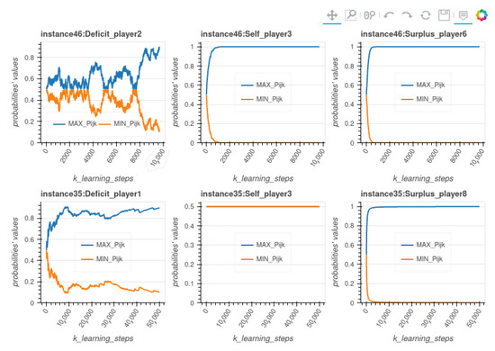
Figure 3.
Examples of stochastic vectors evolution for two instances.
The learning time is therefore mainly used by the players in Deficit to arbitrate between the use of their stock and the use of SG. As illustrated by curves concerning Instance 35 in the figure, the instances that do not stabilize see the probabilities of the actors in state Self remaining at during the training, which has a negative impact on the average of the best probabilities of each actor (even if this situation does not prevent the instance from finally choosing a Nash equilibrium). Indeed, in these instances, some actors in State Self are such that and ; for these actors, the two strategies are equivalent, with a utility equal to zero. These are the worst cases for the effectiveness of learning, but RL still succeeds in determining the Nash equilibrium.
We consider also another type of instances with 10 actors for which there does not systematically exist pure Nash equilibria.
- 4 actor in State Deficit with , , .
- 3 actor in State Self with two possible situations with probability : one in which , and uniformly chosen in ; the other in which , and uniformly chosen in .
- 3 actor in State Surplus with , , .
We also consider and for each actor . Note that , , and are the same as in the previous instance generation scenario.
In the simulation, we run at most 30,000 learning steps in each of the 50 period instances. In this instance set, only 4 instances admit a Nash equilibrium, with the same properties as the ones of stabilizing instances of the previous scenario. As regards the 6 other instances, there is no stabilization. The ratio of values of given by RL and the one given by TEM varies between and , knowing that the mean value of by RL is equal to for these six instances. The difference between the actor profiles given by RL and TEM is that the values of is less in TEM profiles than in RL ones, ie that these actors in State Surplus are solicited by SG upon to contribute beyond their own interest, which contradicts the objectives of the proposed model.
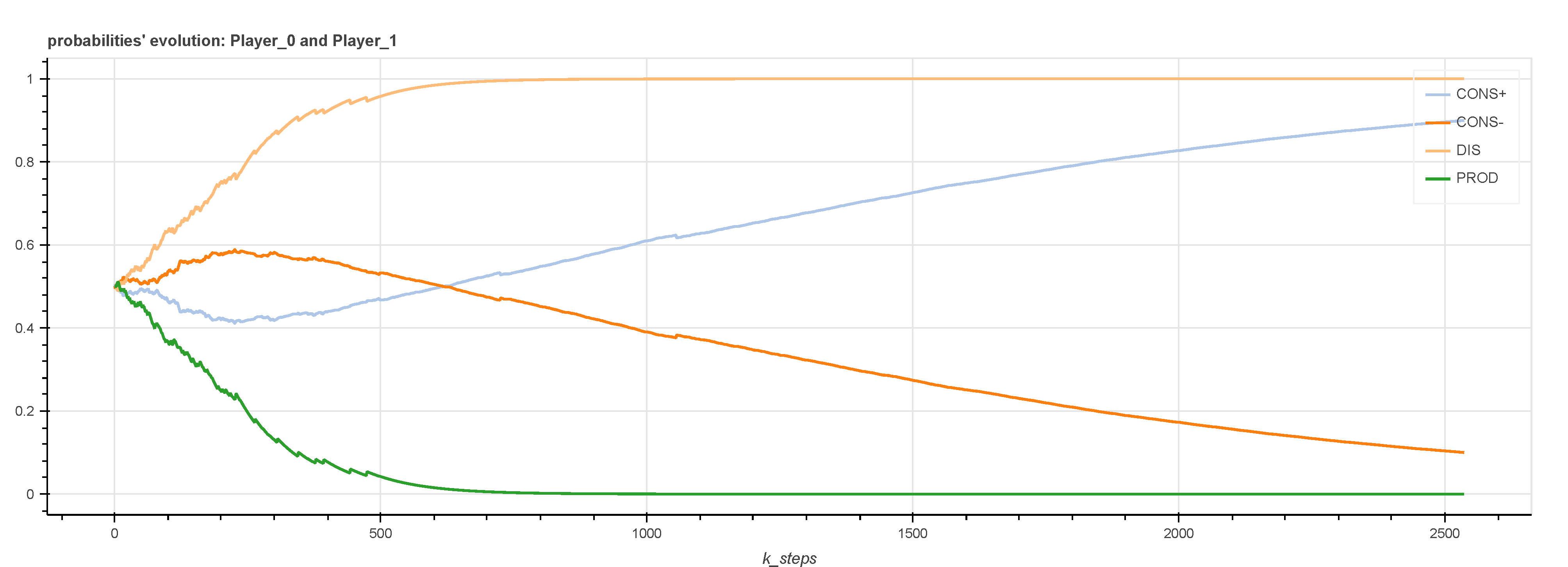
Finally, we focus on the evolution of the strategy probabilities during the execution of RL for a two-player instance resulting from the proof of Lemma 1. This instance is defined by
- , , and ,
- , , and ,
- , , , and .
In this case where there is no Nash equilibrium, as shown in Figure 4 Evolution of the probabilities of the strategies of the two actors during RL steps, at the beginning of learning, actor 2 quickly confirms its choice of the DIS strategy, that is to say to favor its stock. It is the consequence of actor 1 first favoring the , which leads it to use all the energy that actor 2 overproduces. Therefore, actor 2 does not derive any benefit from a sale of electricity to EPO.
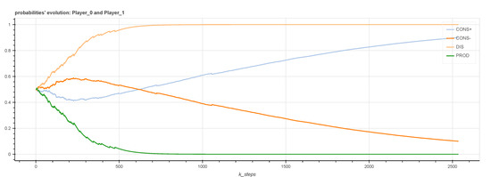
Figure 4.
Evolution of the probabilities of the strategies of the two actors during RL steps.
When actor 1 eventually learns to prioritize its stock (strategy ), actor 2’s decision to choose DIS has reached a probability too high to be challenged by RL, even if it begins to decline again slightly. In this example, it is therefore the initial decision of the actor in the Surplus state, which dominates the learning process.
Thus, to summarize all this RL performance evaluation, through all these experiments, it appears that when a Nash equilibrium exists and corresponds to an optimal value of , RL succeeds in determining it (note that it appears experimentally difficult to generate instances having a Nash equilibrium but which is not an optimal). Among these instances, those that do not stabilize are those in which the two strategies are equivalent for a certain number of actors in state Self, without this preventing RL from determining the Nash equilibrium. When a Nash equilibrium does not exist, RL determines a profile, which remains efficient in terms of compare to the one provided by TEM, without sacrificing the situation of actors in Surplus state in particular. This experimentation shows the interest to use RL in this context, and it is now a question of evaluating the performance of RL for a series of periods, which is studied in the next section.
3.2. Multi-Periods Simulation
3.2.1. Instances Generation
We consider the following scenario of instances generation over consecutive periods, where the situation of each of these actors at any period is determined from the one at period by considering one of the transition automata given in Figure 5 Transition states automata for instances generation.
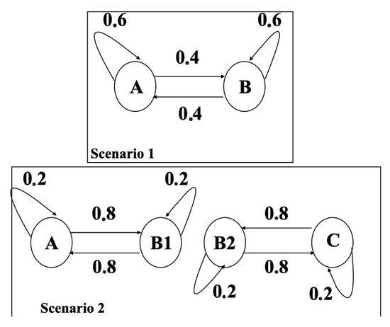
Figure 5.
Transition states automata for instances generation.
Data for each actor at each period t are generated as follows. Consider first that each actor is in one of four situations defined as follows:
- Situation A: and is uniformly chosen in ; .
- Situation B1: and is uniformly chosen in ; .
- Situation B2: and is uniformly chosen in ; .
- Situation C: , ; .
Considering all the periods, the average electricity quantity that is consumed per period by actors is equal to 400 and the average produced one is 380.
This instance generation tends to represent a situation in which a smart grid connects two types of actors. On the one hand, players that are not very productive relatively to their needs (situations A and B1), typically old collective housing or administrative buildings, on the other hand players with high consumption but with significant production capacities and energy storage (situations B2 and C), typically eco-responsible buildings or recent industrial buildings.
For , we consider initially 8 actors in Situation A (with initial stock ), 5 actors in Situation (with initial stock ), 5 actors in Situation (with initial stock ) and 8 actors in Situation C (with initial stock ).
Finally, as in Section 3.1—Learning performance analysis, we consider , , and .
3.2.2. Performances Evaluation
Considering each of the three scenario above, we generate, for each actor, values and for 50 consecutive periods. On each of the such obtained three sequences of values, we compare at each period the performances of RL, a Systematic algorithm (SyA) and a Selfish-deterministic algorithm (SDA). It should be noted that since the methods we propose in this article do not consist in constructing precise predictions of consummations and productions, but rather in calculating actions that tend to optimize a controlled distributed system, based on feedback from the environment of the system, we think that the performance of such a system cannot be summed up in a single global indicator (as for example the accuracy index of a predictive algorithm using statistical learning methods such as Deep Learning). Several parameters must be considered together in order to decide which solution is the best fit. We therefore propose here to take into account three indicators evaluating learning performance (Aperf), effective revenue (ER) and virtual revenue (VR), as defined below.
Regarding RL, we consider a maximum number of 10,000 learning steps; indeed Section 3.1—Learning performance analysis shows that even if there is no stabilization before 10,000 steps, the obtained profile is the same as the one after 50,000 steps. The purpose of these algorithms is to determine a strategy profile for actors at each period.
The Systematic algorithm fixes mode for any actor in State Deficit and mode for any actor in States Self or Surplus; this algorithm consists of having each actor systematically feeding or using its stock.
The Selfish-deterministic algorithm (SDA, Algorithm 1) is defined as follows:
| Algorithm 1: SDA |
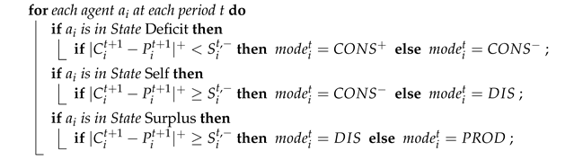 |
In this algorithm, at each period, each actor unilaterally manages its stock considering its needs in the next period.
For each algorithm, we focus on the average value of over all periods. is the utility of actor at period t, considering its benefit , cost and stock incentive (see Section 2.2.1 and Section 3.1). Moreover, for each of the two methods we focus on the values of the Effective Revenue , and the Virtual Revenue , i.e., the one obtain by considering virtual prices and at each period ; remind also that is the real economic balance (see Section 2.1.4—A pricing model for a smart grid) and that and are internal benefit and cost of actor respectively (see Section 2.1.2—Action modes of each actor).
Finally, to evaluate if the situations obtained in each period by RL do not disadvantage the actors in state Surplus, compared to situations obtained by SDA, we define two partial metrics concerning . We thus also define experimentation parameters and , where and are the values of restricted to players initially in Situations A and B1 and the ones in Situations B2 and C, respectively, and where similarly and are the values when using SDA.
The experimentation provides the metric values presented in the following Table 3.
Table 3.
Performance comparison of learning algorithms.
These results show first of all that the SyA method has slightly better performances than those of SDA concerning ER, which seems to indicate that a selfish approach systematically favoring the current stock of each actor is more effective than a deterministic approach aiming to keep into account needs of future stock and sharing within SG. This is no longer the case when such a context is handled by RL, which gives the best performances concerning ER. It should also be noted that the differences in values of V between on the one hand RL and on the other hand SyA and SDA show that these two last methods provide strategic profiles of very poor performances in the sense of the game defined within SG.
Finally, we note that concerning , which calculates the profit in the game virtual economic model of SG, SyA is more efficient than RL because it converges towards profiles that are not Nash equilibria and which, therefore, appear less efficient in terms of real profits (ER). In all the periods generated on the basis of the instance generation scenario described above, it therefore clearly appears that the use of a reinforcement learning method is necessary to allow all the actors of the smart grid to converge towards a less costly situation for all, while preserving the independence of decision of each.
Moreover, the couples of values are equal to . This shows that when considering the objective of keeping account for future stock needs and sharing within the smart grid, with SDA, the overproduction of actors in Situations B2 and C is totally solicited by SG to provide as much energy as possible to the actors in states Situations A and Situations B1, which then have a very low cost to pay. With RL, we see that the interest of each over-productive actor (states Situations B2 and C) is preserved, which increases the cost of other actors. But overall the cost paid by SG to EPO is falling with RL as seen previously. As indicated in Section 2.1.4—A pricing model for a smart grid, a cost allocation solution between actors to globally distribute the cost of the smart grid on each actor could also be considered from the result provided by RL.
3.3. Technical Implementation and Code Performance
Simulations and learning algorithms were implemented on a computer composed of i7-10870H CPU @ 2.20GHz, 8 cores, 16 threads, 64Go RAM. Both are implemented using Python 3.8, with libraries = NumPy (1.20.1) and Pandas (1.2.4).
Even though the system is distributed by nature, simulations for all agents are centralized, in order to compute values of the utility functions. On one period with 50 agents, and 50,000 learning steps for each agent, one simulation takes between 30 min and 1 h. It should be noted that what takes most computing time is the computation of all function utility values.
4. Conclusions
In this article, we proposed a distributed and autonomous decision model based on game theory of a smart grid interconnecting prosumers, associated with an internal economic virtual model that must converge during the execution time towards a real economic model imposed by an external energy supplier (EPO). We show that, by integrating a forecast of the necessary energy stock, the use of learning techniques by reinforcement allows convergence on economically relevant situations for the smart grid while respecting the interests of each prosumer.
When considering a single period of time, these learning approaches proved to be optimal in terms of the energy consumption for all the instances that we considered and allowed for reducing energy costs for all actors of the smart grid. When learning is done across several time periods, it was more efficient than both a simple deterministic algorithm that feeds or uses its stock and a deterministic selfish algorithm that uses a consumption forecast. Moreover, convergence time, which is often an issue with reinforcement learning, remained low here.
As a first approach, the physical operation of smart grids was considered as being able to respond to any set of actions by prosumers without problems in the distribution capacity. Thus, we assumed that the smart grid is able to meet any demand for power distribution. An extension of our approach will have to take into account the dynamic configuration of the network, meaning that the capacity of its components must be able to adapt to each set of prosumer demands. The proposed RL approach will then have to be coupled with a dynamic configuration algorithm of the smart grid topologies, inspired, for example, by [39].
We also assume that the smart grid does not experience any failures or malfunctions. Such malfunctions would impact the actions chosen by each actor and would therefore imply a change of strategic profile "on the fly" imposed by the control of the smart grid by real-time processing when the energy distribution faults are perceived by prosumers. From the point of view of the model to be considered, such failures could follow a stochastic model (for example based on Bayesian networks).
Moreover, since, in this article, we wanted to demonstrate the relevance of an approach using reinforcement learning based on a game model for the distributed management of a smart grid interconnecting prosumers, production and consumption data were considered certain. It would be interesting in future work to perform a sensitivity analysis in order to study the robustness of this approach in the face of the uncertainty of the energy production and consumption data. As already studied in other fields of application, it will be a question in particular of developing RL methods capable of adapting to elastic data considering production and consumption and modeled by stochastic processes.
Finally, in typical smart grids, some prosumers may include electric car charging stations. These charging stations have a significant impact on the management of the configuration of the smart grid, since the energy stored at one point of the network can be relocated (minus a certain consumption made by the electric vehicle during its movement) to another point of gate entrance. In addition, all the energy behaviors of these prosumers depend on the road topology on the territory covered by the smart grid (or even wider), which must therefore be taken into account. Further work could be carried out in order to learn about these types of profiles.
Author Contributions
D.B., B.C.-B. and W.E. have contributed equally to the work of modeling, theoretical analysis and experimentation. All authors have read and agreed to the published version of the manuscript.
Funding
This research was part of GPS (Grid Power Sustainability) project funded by European Regional Development Fund grant number IF0011058.
Institutional Review Board Statement
Not applicable.
Informed Consent Statement
Not applicable.
Conflicts of Interest
The authors declare no conflict of interest.
References
- Calvillo, C.; Sánchez-Miralles, A.; Villar, J. Energy management and planning in smart cities. Renew. Sustain. Energy Rev. 2016, 55, 273–287. [Google Scholar] [CrossRef] [Green Version]
- IRENA. Global Energy Transformation: A Roadmap to 2050; Report of International Renewable Energy Agency; The International Renewable Energy Agency (IRENA): Abu Dhabi, United Arab Emirates, 2018; ISBN 978-92-9260-059-4. [Google Scholar]
- Amicarelli, E.; Tran, T.; Bacha, S. Flexibility service market for active congestion management of distribution networks using flexible energy resources of microgrids. In Proceedings of the 2017 IEEE PES Innovative Smart Grid Technologies Conference Europe (ISGT-Europe), Torino, Italy, 26–29 September 2017; pp. 1–6. [Google Scholar]
- Milchtaich, I. Congestion Games with Player-Specific Payoff Functions. Games Econ. Behav. 1996, 13, 111–124. [Google Scholar] [CrossRef] [Green Version]
- Chien, S.; Sinclair, A. Convergence to approximate Nash equilibria in congestion games. Games Econ. Behav. 2011, 71, 315–327. [Google Scholar] [CrossRef]
- Sastry, P.; Phansalkar, V.; Thathachar, M. Coalitional Game Theory for Cooperative Micro-Grid Distribution Networks. In Multiagent System Technologies; Lecture Notes in Computer Science; Springer: Berlin/Heidelberg, Germany, 2011; Volume 8076. [Google Scholar]
- Osborne, M. An Introduction to Game Theory; Oxford University Press: Oxford, UK; New York, NY, USA, 2004. [Google Scholar]
- Palombarini, J.A.; Martínez, E.C. Closed-loop Rescheduling using Deep Reinforcement Learning. IFAC-PapersOnLine 2019, 52, 231–236. [Google Scholar] [CrossRef]
- Göhrt, T.; Griesing-Scheiwe, F.; Osinenko, P.; Streif, S. A reinforcement learning method with closed-loop stability guarantee for systems with unknown parameters. IFAC-PapersOnLine 2020, 53, 8157–8162. [Google Scholar] [CrossRef]
- Carli, R.; Cavone, G.; Pippia, T.; Schutter, B.D.; Dotoli, M. A Robust MPC Energy Scheduling Strategy for Multi-Carrier Microgrids. In Proceedings of the 2020 IEEE 16th International Conference on Automation Science and Engineering (CASE), Hong Kong, China, 20–21 August 2020; pp. 152–158. [Google Scholar] [CrossRef]
- Nassourou, M.; Blesa, J.; Puig, V. Robust Economic Model Predictive Control Based on a Zonotope and Local Feedback Controller for Energy Dispatch in Smart-Grids Considering Demand Uncertainty. Energies 2020, 13, 696. [Google Scholar] [CrossRef] [Green Version]
- Ibars, C.; Navarro, M.; Giupponi, L. Distributed Demand Management in Smart Grid with a Congestion Game. In Proceedings of the 2010 First IEEE International Conference on Smart Grid Communications, Gaithersburg, MD, USA, 4–6 October 2010; pp. 495–500. [Google Scholar]
- Zhu, Z.; Tang, J.; Lambotharan, S.; Chin, W.; Fan, Z. An integer linear programming and game theory based optimization for demand-side management in smart grid. In Proceedings of the 2011 IEEE GLOBECOM Workshops (GC Wkshps), Houston, TX, USA, 5–9 December 2011; pp. 1205–1210. [Google Scholar]
- Mohsenian-Rad, A.; Wong, V.W.S.; Jatskevich, J.; Schober, R.; Leon-Garcia, A. Autonomous Demand-Side Management Based on Game-Theoretic Energy Consumption Scheduling for the Future Smart Grid. IEEE Trans. Smart Grid 2010, 1, 320–331. [Google Scholar] [CrossRef] [Green Version]
- Horta, J.; Altman, E.; Caujolle, M.; Kofman, D.; Menga, D. Real-time enforcement of local energy market transactions respecting distribution grid constraints. In Proceedings of the 2018 IEEE International Conference on Communications, Control, and Computing Technologies for Smart Grids (SmartGridComm), Aalborg, Denmark, 29–31 October 2018; pp. 1–7. [Google Scholar]
- Tushar, W.; Zhang, J.A.; Smith, D.B.; Thiebaux, S.; Poor, H.V. Prioritizing consumers in smart grid: Energy management using game theory. In Proceedings of the 2013 IEEE International Conference on Communications (ICC), Budapest, Hungary, 9–13 June 2013; pp. 4239–4243. [Google Scholar]
- Samadi, P.; Mohsenian-Rad, A.; Schober, R.; Wong, V.W.S.; Jatskevich, J. Optimal Real-Time Pricing Algorithm Based on Utility Maximization for Smart Grid. In Proceedings of the 2010 First IEEE International Conference on Smart Grid Communications, Gaithersburg, MD, USA, 4–6 October 2010; pp. 415–420. [Google Scholar]
- Fang, X.; Wang, J.; Song, G.; Han, Y.; Zhao, Q.; Cao, Z. Multi-Agent Reinforcement Learning Approach for Residential Microgrid Energy Scheduling. Energies 2020, 13, 123. [Google Scholar] [CrossRef] [Green Version]
- Lu, R.; Hong, S.H. Incentive-based demand response for smart grid with reinforcement learning and deep neural network. Appl. Energy 2019, 236, 937–949. [Google Scholar] [CrossRef]
- Samadi, P.; Schober, R.; Wong, V.W.S. Optimal energy consumption scheduling using mechanism design for the future smart grid. In Proceedings of the 2011 IEEE International Conference on Smart Grid Communications (SmartGridComm), Brussels, Belgium, 17–20 October 2011; pp. 369–374. [Google Scholar]
- Apostolopoulos, P.A.; Tsiropoulou, E.E.; Papavassiliou, S. Demand Response Management in Smart Grid Networks: A Two-Stage Game-Theoretic Learning-Based Approach. Mob. Netw. Appl. 2018, 26, 548–561. [Google Scholar] [CrossRef] [Green Version]
- Deng, R.; Yang, Z.; Hou, F.; Chow, M.; Chen, J. Distributed Real-Time Demand Response in Multiseller–Multibuyer Smart Distribution Grid. IEEE Trans. Power Syst. 2015, 30, 2364–2374. [Google Scholar] [CrossRef]
- Lu, T.; Chen, X.; McElroy, M.B.; Nielsen, C.P.; Wu, Q.; He, H.; Ai, Q. A Reinforcement Learning-Based Decision System For Electricity Pricing Plan Selection by Smart Grid End Users. IEEE Trans. Smart Grid 2020, 12, 2176–2187. [Google Scholar] [CrossRef]
- Saad, W.; Han, Z.; Poor, H.V. Coalitional Game Theory for Cooperative Micro-Grid Distribution Networks. In Proceedings of the 2011 IEEE International Conference on Communications Workshops (ICC), Kyoto, Japan, 5–9 June 2011; pp. 1–5. [Google Scholar]
- Hammad, E.; Farraj, A.; Kundur, D. Cooperative microgrid networks for remote and rural areas. In Proceedings of the 2015 IEEE 28th Canadian Conference on Electrical and Computer Engineering, Halifax, NS, Canada, 3–6 May 2015; pp. 1572–1577. [Google Scholar]
- Aladdin, S.; El-Tantawy, S.; Fouda, M.; Tag Eldien, A. MARLA-SG: Multi-Agent Reinforcement Learning Algorithm for Efficient Demand Response in Smart Grid. IEEE Access 2020, 8, 210626–210639. [Google Scholar] [CrossRef]
- Roesch, M.; Linder, C.; Zimmermann, R.; Rudolf, A.; Hohmann, A.; Reinhart, G. Smart Grid for Industry Using Multi-Agent Reinforcement Learning. Appl. Sci. 2020, 10, 6900. [Google Scholar] [CrossRef]
- Massadi, M.; Abu-Rub, H.; Refaat, S.; Chihi, I.; Oueslati, F. Deep Learning in Smart Grid Technology: A Review of Recent Advancements and Future Prospects. IEEE Access 2021, 9, 54558–54578. [Google Scholar] [CrossRef]
- Zhang, R.; Yang, S.; Zhang, Q.; Xu, L.; He, Y.; Zhang, F. Graph-based few-shot learning with transformed feature propagation and optimal class allocation. Neurocomputing 2022, 470, 247–256. [Google Scholar] [CrossRef]
- Cros, S.; Badosa, J.; Szantaï, A.; Haeffelin, M. Reliability Predictors for Solar Irradiance Satellite-Based Forecast. Energies 2020, 13, 5566. [Google Scholar] [CrossRef]
- Loni, A.; Parand, F.A. A survey of game theory approach in smart grid with emphasis on cooperative games. In Proceedings of the 2017 IEEE International Conference on Smart Grid and Smart Cities (ICSGSC), Singapore, 23–26 July 2017; pp. 237–242. [Google Scholar] [CrossRef]
- Piao, R.; Lee, D.J.; Kim, T. Real-Time Pricing Scheme in Smart Grid Considering Time Preference: Game Theoretic Approach. Energies 2020, 13, 6138. [Google Scholar] [CrossRef]
- Saad, W.; Han, Z.; Poor, H.V.; Basar, T. Game-Theoretic Methods for the Smart Grid: An Overview of Microgrid Systems, Demand-Side Management, and Smart Grid Communications. IEEE Signal Process. Mag. 2012, 29, 86–105. [Google Scholar] [CrossRef]
- Sperstad, I.B.; Korpås, M. Energy Storage Scheduling in Distribution Systems Considering Wind and Photovoltaic Generation Uncertainties. Energies 2019, 12, 1231. [Google Scholar] [CrossRef] [Green Version]
- Carli, R.; Dotoli, M. Cooperative Distributed Control for the Energy Scheduling of Smart Homes with Shared Energy Storage and Renewable Energy Source. IFAC-PapersOnLine 2017, 50, 8867–8872. [Google Scholar] [CrossRef]
- Xu, J.; Yan, C.; Xu, Y.; Shi, J.; Sheng, K.; Xu, X. A Hierarchical Game Theory Based Demand Optimization Method for Grid-Interaction of Energy Flexible Buildings. Front. Energy Res. 2021, 9, 500. [Google Scholar] [CrossRef]
- Maschler, M.; Solan, E.; Zamir, S. Repeated Games; Cambridge University Press: Cambridge, MA, USA, 2013. [Google Scholar]
- Sastry, P.; Phansalkar, V.; Thathachar, M. Decentralized Learning of Nash Equilibria in Multi-Person Stochastic Games with Incomplete Information. IEEE Trans. Syst. Man Cybern. 1994, 24, 769–777. [Google Scholar] [CrossRef] [Green Version]
- Barth, D.; Mautor, T.; de Moissac, A.; Watel, D.; Weisser, M.A. Optimisation of electrical network configuration: Complexity and algorithms for ring topologies. Theor. Comput. Sci. 2021, 859, 162–173. [Google Scholar] [CrossRef]

Publisher’s Note: MDPI stays neutral with regard to jurisdictional claims in published maps and institutional affiliations. |
© 2022 by the authors. Licensee MDPI, Basel, Switzerland. This article is an open access article distributed under the terms and conditions of the Creative Commons Attribution (CC BY) license (https://creativecommons.org/licenses/by/4.0/).