Article

The Role of Pre-Commitments and Engle Curves in Thailand’s Aggregate Energy Demand System

by
Kannika Duangnate
1,* and
James W. Mjelde
2
1
Faculty of Economics, Chiang Mai University, Chiang Mai 50200, Thailand
2
Department of Agricultural Economics, Texas A&M University, College Station, TX 77843, USA
*
Author to whom correspondence should be addressed.
Energies 2022, 15(4), 1578; https://doi.org/10.3390/en15041578
Submission received: 17 January 2022 / Revised: 13 February 2022 / Accepted: 14 February 2022 / Published: 21 February 2022

Abstract

:
In the present paper, an investigation into Thailand’s energy demand is performed to determine if: (1) a linear or nonlinear Engel curve better explains the relationship between income and energy consumption, and (2) systems with pre-commitments better model energy consumptions. Four demand systems are estimated: an almost ideal demand system (AIDS), the quadratic almost ideal demand system (QAIDS), generalized almost ideal demand system (GAIDS), and the generalized quadratic almost ideal demand system (GQAIDS). Elasticities are calculated for policy implications. The empirical results suggest that models considering pre-commitments and nonlinear Engel curves may be slightly more appropriate for Thailand’s energy system, from both statistic and economic standpoints. Statistical inferences appear to favor the GQAIDS model based on the encompassing results. Economic reasonability also appears to favor the GQAIDS model, in particular, petroleum products, as it provides results consistent with the notions of precommitments and fuel substitutability found in previous studies. Most of the previous studies in various forms have shown that the demand for petroleum products is relatively inelastic to price in Thailand. The current study, however, finds that own-price elasticities of uncompensated demand for petroleum products are almost unitary, which is relatively more elastic than most of the previous studies. As such, further studies are required and the price-based policy on petroleum products targeting the reduction in petroleum product dependence must be implemented with caution.

1. Introduction

Energy consumption is a key indicator of economic growth, not only in industrialized/developed countries but also in developing countries. Thailand, a developing country, is no exception. Thailand is dependent on energy imports, which, along with consumption and expenditures, have been increasing over time. Total energy imports increased from THB 89.9 billion in 1994 to THB 1069.8 billion in 2019 [1]. In 2019, Thailand imported 49.8% of its total final energy consumption [1].
Although energy consumption has been increasing over time, short run energy consumption levels only deviate slightly, despite the fluctuations in energy prices. Studies have found inelastic price elasticities for energy consumption in Thailand, and generally suggest that energy demand is less sensitive to price in the short run than in the long run [2,3,4]. Energy sources are purchased in advance for manufacturing/industrial production. Further, energy consumers, by their choice of, for example, technology, appliances, and transportation modes, commit to using a fixed amount of energy in the short run, regardless of their work and residential locations. Such consumption levels that are irresponsive to price are considered as pre-commitments [5]. In the long run, in response to energy prices, energy consumers can alter or move manufacturing production, add insulation, and purchase more energy efficient appliances.
Previous estimated elasticities, however, do not consider the potential influence of pre-commitments on energy consumption in Thailand. Without considering pre-commitments, estimated elasticities maybe inaccurate leading to potentially questionable policy implications. Moreover, most previous studies of Thailand employ models, such as translog or log-linear, which have been contested on a theoretical basis [6,7].
Energy demand may be more precisely estimated by accounting for pre-committed consumption. A study, ref. [8], suggests that policy implications after accounting for pre-commitments in the U.S. aggregate energy demand system differ from models that do not consider pre-commitments. The study reveals that the system with pre-commitments explains the U.S. energy demand system better than the system without pre-commitments. Policy makers need to be aware of that energy demand is much less sensitive to price when the consumption is near pre-commitment levels. The authors of [8] (p. 406) claim that “… if pre-commitments are a legitimate assumption, larger price changes are necessary to achieve a given policy objective than if there no pre-commitments.” It is not clear, however, if considering pre-commitments in developing countries would help policy formulation.
The relationship between expenditures on energy consumption and household income, Engel curve, is an important consideration. Previous studies in Thailand generally assumed a linear in logarithm Engel curve; however, studies suggest that the curve maybe nonlinear for consumer goods [9]. Since assuming a linear Engel curve and ignoring pre-commitments may cause a suggested policy to be ineffective, the objective of this study is to investigate Thailand’s energy demand to determine if: (1) a linear or nonlinear Engel curve better explains the relationship between income and energy consumption, and (2) systems with pre-commitments better model energy consumptions. To achieve these objectives, four demand systems are estimated: almost ideal demand system (AIDS), the quadratic almost ideal demand system (QAIDS), generalized almost ideal demand system (GAIDS), and the generalized quadratic almost ideal demand system (GQAIDS). The quadratic models explicitly assume a nonlinear Engel curve, whereas the generalized models explicitly consider pre-commitments. The comparisons of AIDS to QAIDS and GAIDS to GQAIDS determine if a nonlinear Engel curve provides additional explanatory power over a linear curve. The importance of pre-commitments in helping to explain Thailand’s energy demand are examined by comparing GAIDS to AIDS and GQAIDS to QAIDS. The pre-commitments in the models are treated as perfectly inelastic, although the reality is that pre-commitments are almost perfectly inelastic as people always have some choices. The models are compared both on a statistical basis and economic reasonability of the estimated elasticities.
Elasticities are presented for the policy implications. To ease the dependency on energy imports and address the pollution issues, the policies targeting decreases in energy consumption should be considered. The validity of assumptions on the Engel curve shape and pre-commitments in explaining Thailand’s energy demand system and resulting elasticities is important in developing price-based policies. To the authors’ knowledge, this is the first study of Thailand’s energy consumption, explicitly incorporating pre-commitment consumptions with different Engle curves.

2. Thailand’s Energy System

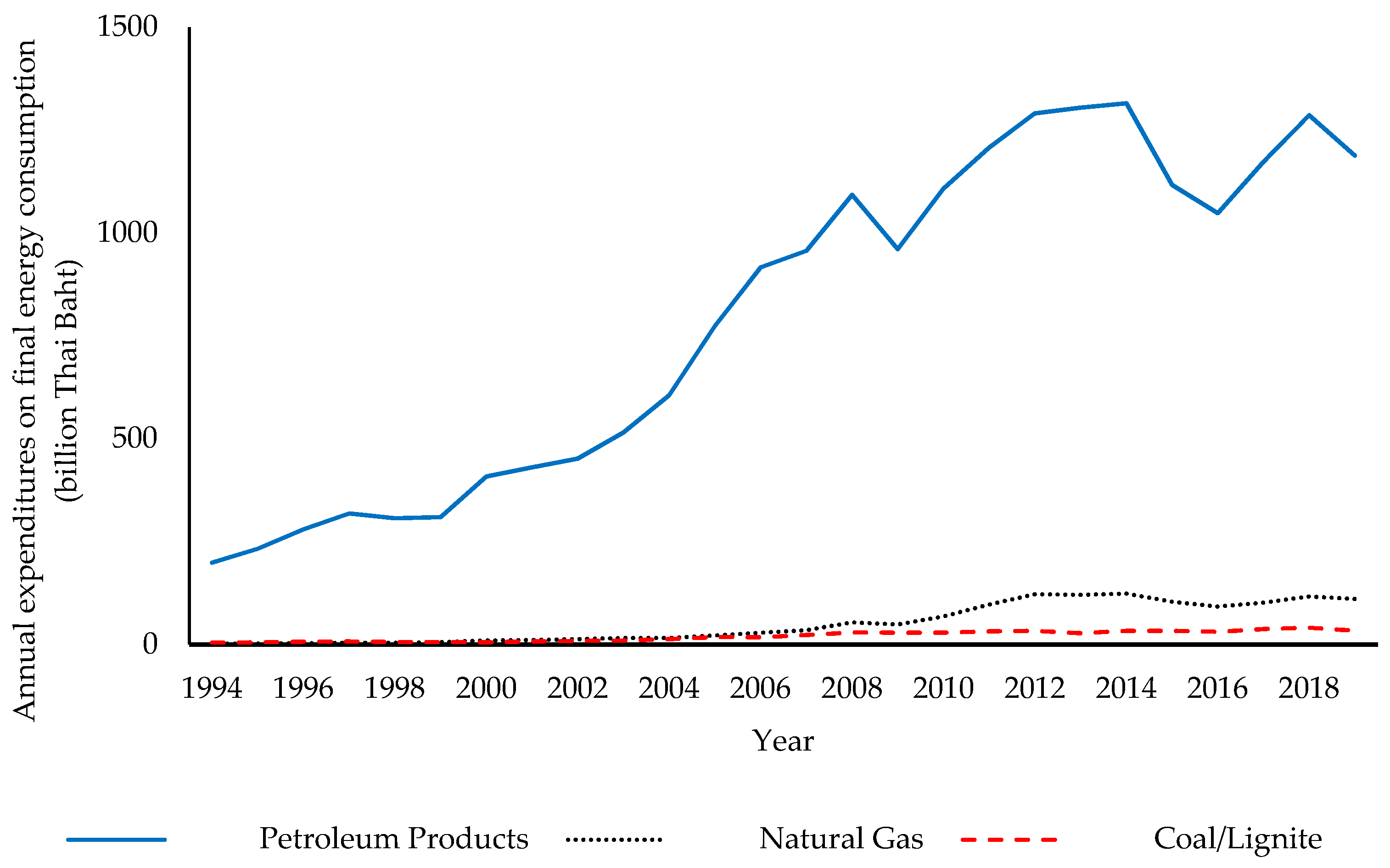
Both the annual expenditures on final energy consumption and gross domestic product (GDP) have been increasing over time in Thailand (Figure 1). The final energy expenditures on the petroleum products are by far the largest among the energy sources (Figure 2). Petroleum made up 55.4% of the total final expenditures in 2019 [1]. Similar to the expenditures on final energy consumption, energy imports are also increasing (Figure 3); the variation in energy imports shares a similar pattern with that of the energy consumption expenditures. Not surprisingly, crude oil imports have the largest import shares because domestic crude oil production cannot satisfy domestic consumption. Thailand crude oil production was 19.6% of the consumption oil products in 2019 [10].
Such a high dependency on energy imports makes Thailand’s economy vulnerable to world oil market fluctuations. Such vulnerability suggests that Thailand policy makers may want to devise a national energy management program that, in part, considers the consumer’s response to price changes. As such, an understanding of how responsive consumers are to changes in energy price, i.e., price elasticities of energy demand, is necessary. Thailand is dependent on energy imports, especially crude oil. Aiming to lessen the dependency on energy imports and the environmental issues, helps to explain why most of recent studies on energy systems in Thailand focus on reducing CO2 emissions from energy usage.

3. Thailand Energy Demand Modeling

Energy demand modeling plays an important role in designing energy policies to address numerous energy issues, including national security and pollution, two important societal challenges. Numerous methodologies have been used to model the energy demand system [11,12]. Ref. [11] classify energy demand models as either top-down or bottom-up models. Based on economic theory, top-down models use econometric techniques to estimate energy demand at an aggregate level and examine if the estimated results are consistent with economic theory. Bottom-up models use comprehensive engineering models to characterize the energy system for the end-uses. To bridge the gap between the two methodologies, hybrid models incorporating features of the two models were developed.
Econometric models found statistically significant relationships between economic factors, such as GNP, energy price, population, technological development, and energy efficiency and aggregate energy demand [11,12]. Studies in developing countries, however, find that energy prices are not a substantial factor affecting energy demand, which might be explained by energy price regulations [11] or energy demand analyses without considering the pre-commitments.
As a result of their high adaptability, bottom-up models, such as the Model of Analysis of Energy Demand (MAED) and the Long-range Energy Alternative Planning (LEAP) model, are widely used to study the energy demand in developing countries. These models, however, fail to capture the price effects on energy demand, implying that they cannot provide price-based policy recommendation [11].

3.1. Bottom-Up Approaches

By reviewing studies (during 2003–2011) of energy system modeling in Thailand, ref. [13] found that technical feasibility and bottom-up modeling studies were the most prevalent in energy study approaches used in examining energy systems in Thailand. Using models, such as the Long-range Energy Alternative Planning (LEAP) model and the Asia–Pacific Integrated Model (AIM), these studies reveal that improvements of energy efficiency and the implementation of renewable energy and advanced technologies will shrink the energy demand and CO2 emissions.
Studies that used the LEAP model include [14,15,16,17]. Both [14,16] found that strategies and technologies in the transportation section can lessen energy consumption and CO2 emissions. Ref. [14], for example, found that the improvement of public transportation and engine technology for the transport sector can reduce energy consumption in 2020 by an equivalent of 635 thousand tons of oil, and 2024 thousand tons of CO2 equivalents. When considering the commercial, industrial, governmental, residential, and transport sectors of the City of Bangkok, ref. [16] found that the most substantial energy savings are in the transport sector. Unlike the strategies concerning the transport sector proposed by [14,16], ref. [17] examined alternative strategies. They find that using ED95 fuel, a mixture comprised of 95% ethanol and 5% additives, can reduce the consumption of fossil fuels. Further, substituting natural gas vehicles by ED95 fuel technology can lessen CO2 emissions. In addition to the transportation sector, energy efficiency improvements and technological advances can lead to energy savings in sectors that include the residential sector, small commercial buildings, and industrial sector [15,16].
Focusing on the long-term energy policies, refs. [18,19] examined whether Thailand’s existing energy efficiency plan (EEP2015) and renewable energy plan (AEDP2015) can achieve the Nationally Determined Contribution (NDC) target of reducing GHG emissions by 20% from the business-as-usual level by 2030. Even though [18,19] considered different sectors, they reached similar conclusions that the implementation of the plans can lead to the achievement of the NDC target. Ref. [18] suggested that energy labeling and monetary incentives are the most effective measures in the building and industrial sectors. Measures suggested by [19] consisted of developing energy efficiency, encouraging the exploitation of renewable energy and advanced technologies, such as carbon capture and storage (CCS), stimulating renewable electricity generation and motivating public awareness in climate change.
Ref. [20] found that emission trading policies can decrease fossil fuel depletion and expand renewable energy. Carbon capture system technologies may lower the GHG emissions, but will reduce renewable energy use, and energy efficiency improvements. Refs. [21,22] suggest other policy measures beyond technology to increase efficiency, in order to decrease energy consumption and increase energy security. These measures include the use of biofuel, and a conversion from private-centric to public-centric transport modes.

3.2. Economic/Econometric Approaches

Studies using economic/econometric approaches to estimate the elasticities for energy commodities in Thailand are listed in Table 1. These studies are primarily at sectoral level(s), in particular, transportation, and not at the national level. One exception is [23], which examined the final energy demand. A wide range of methods and resulting elasticities were found. The methods used ranged from logarithm models, such as log-linear and translog to time series methods of cointegration. Regardless of the sector, the short-run demand for energy sources in Thailand are more inelastic than the long-run demands. Ref. [4], for example, found the income elasticity for gasoline to be 0.35 in the short run and 1.40 in the long run. Most studies use annual data, but some studies have used monthly data [24] and survey data [25].
The studies directed towards the transportation sector include [4,24,25,26]. Ref. [3] examined the short-run and long-run determinants of final oil consumption in seven major economic sectors, one of which is transportation. In comparing the dynamic panel data estimation to the autoregressive distributed lag equilibrium correction framework, they found that the latter approach provided more information than the former. Focusing on road transportation in Thailand, ref. [4] included own prices, real GDP, stock of vehicles, and time trend as the explanatory variables to explain the gasoline and diesel in the static and dynamic models. Dynamic models augment the static model by including lagged demand. The author also employed cointegration and error correction models. Ref. [4] concluded that the demands for gasoline and diesel are predominantly controlled by income rather than price, which suggests that price-based policies would be ineffective in reducing the quantity demanded, and non-pricing policies would be more effective in the long run. By combining log-linear regression models and feed-forward neural network models, ref. [26] revealed that their prediction of transport energy consumption in 2030 was only 61–65% of the level estimated in a previous study using the LEAP model. The difference is attributed to the differing methodologies used, model requirements, and assumptions on future inputs. Estimated from the log-linear regression model, the elasticity of the transport energy demand with respect to GDP is almost unitary at 0.995. Other studies also reported finding near unitary income elasticities. Considering the whole economy, ref. [23] estimated Thailand’s income energy elasticity at 0.923. Similarly, ref. [27] reported a long-run income elasticity of demand for imported crude oil near unity, estimated using a cointegration model. Ref. [27] also found that short-run price elasticity was positive, yet statistically insignificant, and a short-run income elasticity of about one-half of the long-run elasticity.
Using the monthly data and the AIDS model, ref. [24] estimated the price elasticities of demand for transportation fuels to calculate the deadweight loss from the price distortions in Thailand’s transportation fuel market. The authors found that own-price elasticities of demand for all kinds of gasoline and gasohol except diesel are elastic. Cross-price elasticities reveal that Regular 95 is a close substitute to Gasohol 95 E10, but not to E20/E85. This difference is attributed to the combustion engine requirements for gasohol consumption. They suggest that any price-distorting policy tends to induce a greater deadweight loss, as the demands for transportation fuel are more sensitive to price changes than before. Their study reveals that most of the deadweight losses are a result of an intervention in the price of diesel, which has been underpriced, which causes the overconsumption of diesel. Rather than capping the diesel price, ref. [24] suggested imposing an excise tax or corrective tax on transport fuel consumption, and transferring tax revenue to the poor and developing the existing public transportation and the rail transportation systems. Employing the QAIDS approach, ref. [25] used the data of 122,601 households from the Socio-Economic Survey (SES) in the years 2009, 2013 and 2015, to analyze the demand for gasoline, gasohol, liquified petroleum gas (LPG), and diesel used in the transportation sector. Own-price elasticities of the uncompensated and compensated demands for all energy sources are negative, with the compensated demand elasticities in the absolute value being less than uncompensated demand elasticities. Own-price elasticities of uncompensated gasoline and diesel are elastic (greater than 1 in absolute values), while those of gasohol and LPG are inelastic (less than 1 in absolute values). Own-price elasticities of compensated demand for all energy sources except gasoline are inelastic. The authors suggested that a carbon tax would be an effective policy on reducing gasoline and diesel consumption, yet it escalates inequality because the poor are impacted more than the rich. Using household survey data and the QUAIDS model, ref. [25] found the elastic own-price elasticities of demand for gasoline and diesel and the inelastic elasticities for gasohol and LPG.
Focusing on the Thai manufacturing sector, ref. [2] explored the inter-factor and inter-fuel energy demand using the dynamic translog framework. The factors considered in their study are the final energy consumption in the manufacturing sector, labor, and net capital stock, and the fuel types considered were fuel oil, diesel oil, liquefied petroleum gas, electricity, and coal and lignite. They found a weak energy-capital substitutability, but a strong fuel substitutability, especially between diesel and liquefied petroleum gas. Given this substitutability, they suggested that a price-based policy on the liquefied petroleum gas would increase the consumption of liquefied petroleum gas, as a substitute for diesel.
As seen above, the literature on Thailand’s energy consumption/demand uses a wide range of scopes and methodologies. Relying on engineering perceptions, most studies employ the bottom-up or end-use models that focus on the long-run policies. However, these models lack the ability to capture price-induced effects [11,13]. Relying on the econometric approach, most studies employ the translog or the log-linear models that have the limitation that theoretical regularity conditions may not commonly hold [6,7]. Moreover, no study accounts for the pre-commitments.

3.3. Pre-Commitment Consumption and the Engel Curve

The pre-commitment consumption was first introduced by [5], by assuming that a consumer “always buy a necessary set of good” [5] (p. 88), as an attempt to provide an economic interpretation of a constant term in a linear demand system. Ref. [6] inferred the consumption of necessaries as committed consumption, and proposed a generalized version of the AIDS model (GAIDS) by incorporating the committed quantities. These demand models, however, involve the expenditure share Engel curves that are linear in the logarithm of total expenditures. Since the Engel curves for consumption appear to be nonlinear, ref. [9] proposed the QAIDS model in which the Engel curves are a quadratic function of the logarithm of the total expenditures. Generalizing the QAIDS, ref. [28] considered the pre-committed consumption expenditure in the demand system, GQAIDS.
Studies on energy demand have incorporated pre-commitments [8,29,30,31]. In the analyses of [29,30,31], there is no clear discussion on the application of pre-commitment estimates. Ref. [31] found that results from the GAID were preferred, and the global energy demand was inelastic. Further, the authors found that country-specific elasticities differ across time and income levels. Similarly, ref. [8] found that the demand system considering pre-commitments outperforms the system without pre-commitments, in describing aggregate energy demand in the U.S. They find that pre-commitment quantities account for 60% or more of the average energy consumption. To the authors’ knowledge, there are no energy studies employing the GQAIDS.

4. Methods and Data

Empirical demand analysis focused on the application of the Cobb–Douglas and the constant elasticity of substitution functional forms, in which the regularity conditions are globally satisfied, until [32] established the impossibility theorem. Locally flexible functional forms, such as the translog and the AIDS, which can attain theoretical regularity conditions, at a point, became popular alternatives after the establishment of the impossibility theorem; however, these functional forms violate the conditions of the duality theorem as they are locally regular, not globally regular [7]. As noted earlier, different generalizations of the locally flexible AIDS model are estimated to examine the Engel curve shape and appropriateness of pre-commitments. The models are AIDS and GAIDS, which have a linear Engel curve, and QAIDS and GQAIDS, which assume quadratic Engel curves. The QAIDS is one of the flexible functional forms that is globally regular [7]. Further, the GAIDS and GQAIDS explicitly account for pre-commitments. The total expenditures considered are the expenditure on the final energy consumption in Thailand.
The most general form Is the GQAIDS model, which is derived from the traditional AIDS models. The expenditure shares of the GQAIDS are [28],
w i = c i p i μ + μ ¯ μ { α i + j = 1 n γ i j ln p j + β i ln μ ¯ P + λ i β ( p ) [ ln μ ¯ P ] 2 }
where i = 1, 2, 3 (coal and lignite, natural gas, and petroleum products). μ ¯ = μ c p is defined as the supernumerary expenditure, μ is the total expenditure on final energy consumption, p is the vector of 3-energy source prices, c p = i = 1 3 c i p i refers to the pre-committed expenditures, and c i is the pre-commitment parameter for each energy source to be endogenously estimated. λ i represents the effect of the quadratic Engel curves on the expenditure shares and β ( p ) = i = 1 3 p i β i is the Cobb–Douglas price aggregator function [28]. Following [33], this study uses the Stone’s price index of ln P =   i = 1 3 w i ln p i . The restrictions i = 1 n α i = 1 ,   i = 1 n β i = 0 ,   j = 1 n γ i j = 0 ,   γ i j = γ j i , and i = 1 n λ i = 0   are imposed to satisfy the theoretical restrictions of adding-up, homogeneity, and symmetry. The expenditure shares of coal and lignite and natural gas are estimated, while the parameter estimates of the petroleum products are obtained using the theoretical restrictions. Following [8], the fitted total expenditures derived from regressing the observed total expenditures on the three energy prices and gross domestic product ere used, instead of the observed total expenditures to address the endogeneity issues. The autoregressive process was employed to address the serial correlation issues of the residuals. All estimations were performed using the iterated seemingly unrelated regression via SAS Studio (SAS OnDemand for Academics).
To test if the GQAIDS was appropriate or not, we tested whether or not the estimated λ i was significantly different from zero. If the estimated λ i is not significantly different from zero, the model becomes the generalized version of the AIDS (GAIDS) model developed by [6]. The expenditure share of the GAIDS model is
w i = c i p i μ + μ ¯ μ { α i + j = 1 n γ i j ln p j + β i ln μ ¯ P } .
Without pre-commitments, the demand system becomes the traditional AIDS [33]
w i = α i + j = 1 n γ i j ln p j + β i ln μ P .
Once the demand systems are estimated to further explore Thailand’s energy system, the uncompensated, compensated, and Allen (own-price, cross-price, and expenditure) elasticities are estimated. Even though Allen elasticities have been commonly used to measure substitution behavior, the Morishima elasticities, incorporating the ratio of two goods, are also calculated, because Allen elasticities may be uninformative when a demand system is comprised of more than two goods [34].
Because the monthly/quarterly data of the expenditure on primary energy consumption were not available, the present study focused on the final energy consumption. As such, energy consumption in electricity generation was not included. The final consumption values of the three energy sources used were: (1) solid fossil fuel, which is the summation of coal and lignite, (2) petroleum products, which are the summation of LPG, premium and regular gasoline, jet fuel, kerosene, diesel, and fuel oil, and (3) natural gas used in industrial and transport sectors. The monthly final energy consumption in kiloton of oil equivalent (KTOE) were retrieved from [35]. Monthly data on the expenditures on the final energy consumption were provided by the Energy Policy and Planning Office (EPPO), upon the request of the authors. Monthly data were aggregated to quarterly data, because quarterly data are not available for the gross domestic product (GDP). The quarterly data of the GDP chain volume (GDP CVM) (reference year is 2002) are from [36], the Office of the National Economic and Social Development Council (2020). GDP CVM was used to calculate a GDP deflator, which is used to construct the real expenditures on final energy consumption values. The price of each energy source is equal to the real expenditure divided by consumption. Each series contains 108 quarters covering the period of 1993–2019.

5. Results and Discussion

5.1. Statistical Comparisons

The estimation results for the four models are similar in statistical inferences (Table 2). To determine if the Engel curve maybe nonlinear, quadratic models were compared to linear models, QAIDS to AIDS and GQAIDS to GAIDS. Between the QAIDS and the AIDS models, the QAIDS model objective value was slightly smaller than that of AIDS. The adjusted R-squared for the natural gas (coal) equation is slightly larger in the QAIDS (AIDS) than the AIDS (QAIDS) model. Between the GQAIDS and GAIDS models, the objective value was slightly smaller in the GQAIDS model; the adjusted R-squared for both coal and natural gas equations were slightly larger in the GQAIDS than GAIDS model. Individually, two of the three lambdas were statistically significant. In terms of the total number of significant variables explaining the demand (including the lags of shares), the quadratic models had one more variable significant at a p-value of 0.10 than the linear models. Not including the lags, the GQAIDS had one more significant variable than GAIDS, whereas AIDS had one more significant variable than QAIDS.
Encompassing tests on the predicted values of coal and natural gas from the four models were performed by regressing the error term, which is the difference between the observed and predicted share values, on the difference between itself and the error term from the other model [37]. When one model encompasses the other model, it indicates that the other model contains no useful information not presented in the encompassing model. The encompassing test of the QAIDS and AIDS indicates that the QAIDS encompasses the AIDS model. The statistical inference does not strongly suggest either the quadratic or linear Engel curve as the “best” model, but may be slightly favored over a quadratic Engel curve. Other statistical tests and procedures could be applied, but because of the closeness of the models, the inferences will be very similar and there is no obvious winner, statistically, between the models.
Next, the appropriateness of pre-commitments was examined. In comparing non-precommitment models (AIDS and QAIDS) to models that include pre-commitments (GAIDS and GQAIDS), the objective function values are slightly smaller in the pre-commitment models. Adjusted R-squared is slightly larger for the natural gas (coal) equation in the pre-commitment (non-precommitment) models. In both the GQAIDS and GAIDS models, pre-commitment estimated parameters are jointly different from zero (Table 2). All individual pre-commitment parameters in the GQAIDS are statistically significant in explaining the expenditure shares; however, the pre-committed parameter for natural gas in the GAIDS is not statistically significant. The statistically significance of pre-committed parameters in both GQAIDS and GAIDS suggests that Thailand’s energy demand analysis, including pre-commitments, may be a better model. Encompassing results suggest that the two nonlinear Engel curve models encompass the linear models. The GQAIDS encompasses the QAIDS and the GAIDS encompasses the AIDS. The average pre-commitment levels are provided in Table 3. The pre-commitment levels for coal and lignite and petroleum are larger in the GAIDS model than in the GQAIDS model. The average pre-committed consumption of coal and lignite, natural gas, and petroleum products are 38%, 15%, and 64% of the average consumption for QGAIDS and 54%, 11%, and 79% for GAIDS, respectively. The estimated pre-commitments reveal that the dependence of energy demand in Thailand on petroleum, and coal and lignite products’ final consumption for the pre-committed levels, may be unresponsive to price changes in the short run. The only study known to the authors in which pre-commitment levels are provided for energy is [8]. The pre-commitment levels in their study for the United States are 69%, 60%, and 87% for coal, natural gas, and oil, respectively. Pre-commitment levels for coal and lignite and petroleum for Thailand from the GAIDS model are closer to those values given in [8] than for natural gas. It should be noted that this comparison is between a developed country and a developing country with other differences, such as climate, transportation, and size, and the percentages for the U.S. are yearly and not monthly pre-commitments. It appears that pre-commitments seem to be appropriate for Thailand’s energy system from both a statistical and practical standpoint (discussed earlier), but the evidence is not overwhelming.
To compare the four models, the encompassing results suggest that the GQAIDS encompasses the other three models. These results provide support for a system that includes a quadratic Engel curve and pre-commitments.

5.2. Elasticities of Demand

Elasticities of demand for the three energy sources with and without considering pre-commitments are compared to determine which model provides a “better” economic interpretation (Table 4). All elasticities are calculated at the variables’ means. QAIDS yields more elasticities that are statistically significant than GQAIDS. Similarly, AIDS has more significant elasticities than GAIDS. All expenditure elasticities are positive, and all are significant, except for coal and lignite in the GAIDS model. Most expenditure elasticities are approximately unitary. The estimates of the coal and lignite expenditure elasticities range from 0.685 in the GAIDS model to 1.609 in the AIDS model. Natural gas elasticities range from 0.335 in the GQAIDS model to 0.817 in the AIDS model. Although not 100% comparable, the estimated elasticities are in the range presented by previous studies, except maybe coal and lignite expenditure elasticity from the AIDS model. Expenditure elasticities suggest that the coal and lignite, natural gas, and petroleum products are normal goods.
Consistent with the demand theory, the own-price elasticities of uncompensated demand for all energy sources are negative. In the pre-commitment models, only the own-price elasticities for petroleum are statistically significant, whereas in the non-precommitment models, all the own-price elasticities are significant. The own-price elasticities of compensated demand are negative for coal and lignite and natural gas, but positive for the petroleum products. A similar pattern of significance to the uncompensated is observed (although not 100%) in the compensated elasticities. Most of the estimated elasticities of uncompensated demand are more elastic than those of compensated demand in the four models. Because the elasticities are estimated at the variables’ averages, the cross-price elasticities of the estimated compensated demand are not symmetric. The Allen own-price elasticities showed a similar pattern to the uncompensated elasticates. All four models have positive compensated and Allen own-price elasticities of demand for petroleum products; this can be explained why the own-price elasticities of uncompensated demand for petroleum products being close to −1.0 and the average of petroleum product expenditure share is 0.9. The positive own-price elasticities of uncompensated demand for some petroleum products are found in [2,27].
Studying the U.S. aggregate energy demand system, ref. [8] found that the elasticities estimated from models explicitly considering the pre-commitment consumption were more elastic than those estimated from models that did not explicitly consider pre-commitments. This result is consistent with the idea of pre-commitments discussed earlier. Of the 66 comparisons of elasticities between the non- and pre-commitment models, non-precommitment models are more elastic 68% of the time. Expenditure elasticities and uncompensated own- and cross-price elasticities of the demand for only petroleum products estimated from the pre-commitment models are slightly more elastic than those from the non-precommitment models. Uncompensated own-price elasticities for petroleum products estimated from the four models are roughly the same. Most of compensated own- and cross-price and Allen elasticities estimated from the pre-commitment models are relatively less elastic than those from the non-precommitment models; two exceptions being for own-price elasticities for petroleum products with the other two exceptions involving coal and lignite and natural gas.
The uncompensated cross-price elasticities from the four models suggest that all pairs of the three energy sources are complements. In the GQAIDS model, the compensated and Allen cross-price elasticities of all energy-pairs are substitutes. In the other three models, coal and lignite are complements to natural gas, while petroleum products are substitutes for coal and lignite and natural gas. Morishima elasticities from the two quadratic models suggests that all pairs of the three energy sources are substitutes, whereas coal and lignite are the complements to natural gas in the GAIDS and complements to petroleum products in the AIDS. The Allen elasticities may be uninformative when a demand system is comprised of more than two inputs [34]; the Allen elasticities are said to overstate the complementarity relationship, i.e., when two inputs are Allen complements, they are Morishima substitutes [7]. From an economic standpoint, the quadratic Engel curve models seem to explain the final energy consumption in Thailand better than the linear models. Further, the pre-commitment models seem to explain the final petroleum energy consumption in Thailand better than the non-precommitment models, but the non-precommitment models explain coal and lignite and natural gas better.

6. Conclusions

This study raises more questions than it answers for modeling energy demand in developing countries, in general, and Thailand in particular. Is demand estimation by expenditure shares appropriate, and if so, how? Are pre-commitments and nonlinear Engel curves appropriate?
Statistically, all four models are very similar. The differences between the models are found when considering the economic interpretation of the elasticities. Models considering pre-commitments and nonlinear Engel curves may be more appropriate for Thailand’s energy system from both statistic and economic standpoints. Statistical inferences appear to favor the GQAIDS model based on the encompassing results. Economic reasonability also appears to favor the GQAIDS model, in particular, petroleum products, as it provides results consistent with the notions of precommitments and fuel substitutability found in other studies. Most of the previous studies in various forms have shown that the demand for petroleum products is relatively inelastic to price in Thailand. The current study, however, finds that own-price elasticities of uncompensated demand for petroleum products are almost unitary, which is relatively more elastic than most of the previous studies. The own-price elasticities of demand for coal and lignite are relatively more inelastic than that estimated in [2].
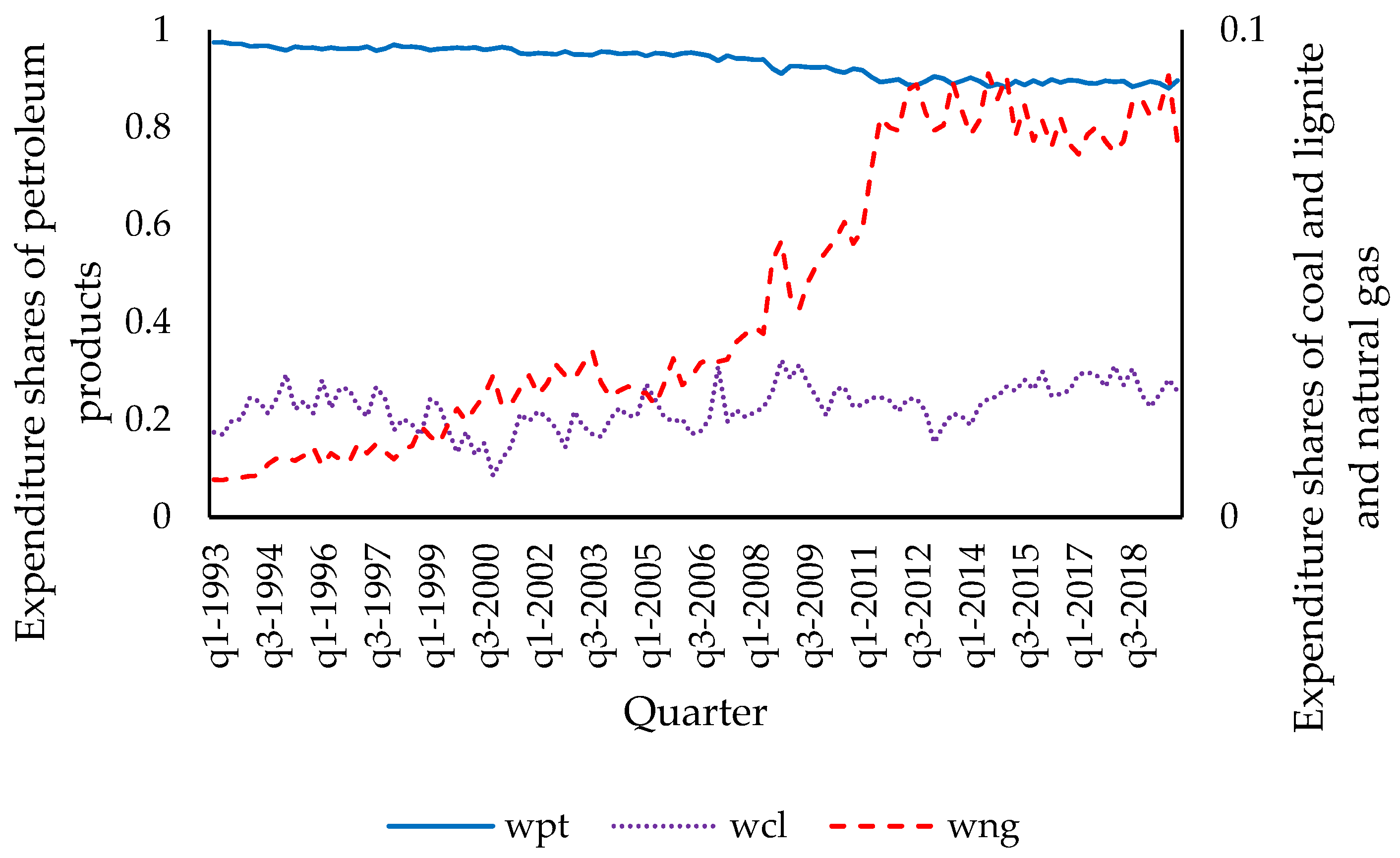
Petroleum products are the dominant energy source in final energy consumption in Thailand. The minimum petroleum product expenditure share is 0.88, while the expenditure share of coal and lignite and natural gas are less than 0.1 (Figure 4). Moreover, the expenditure share of petroleum products signals a downward trend, while that of natural gas signals an upward trend. These may explain why the own-price elasticities of demand for petroleum products from GQAIDS and QAIDS are roughly the same, and why models explicitly considering pre-commitments appear to explain energy consumption in a developed country better than in a developing country. Evidently, further studies are required to address the mentioned questions. Suggested further studies include addressing why the own-price elasticities of demand for petroleum products from GQAIDS and QAIDS are roughly the same, and why models explicitly considering pre-commitments appear to explain energy consumption in a developed country better than in a developing country.
What Thai policy makers could do, while anticipating results from further studies, is to construct a policy reducing the importance of or the dependence on the petroleum products. The price-based policy on petroleum products targeting the reduction in petroleum product consumption must be implemented with caution, as it may be problematic given the indeterminate interpretation of price elasticity of petroleum products; petroleum products are found to be the almost-unitary elastic in this study, in which precommitments are explicitly considered, but inelastic in the literature. Moreover, the price-distorting policy could induce deadweight loss [24]. Given the substitutability between petroleum products and coal and lignite and natural gas, and the relatively low carbon emission of natural gas, a policy encouraging the substitution of natural gas for petroleum products should be employed.

Author Contributions

Conceptualization, K.D. and J.W.M.; methodology, K.D.; software, K.D.; validation, K.D. and J.W.M.; formal analysis, K.D. and J.W.M.; investigation, K.D.; resources, K.D.; data curation, K.D.; writing—original draft preparation, K.D.; writing—review and editing, K.D. and J.W.M.; visualization, K.D.; supervision, J.W.M.; project administration, K.D.; funding acquisition, K.D. All authors have read and agreed to the published version of the manuscript.

Funding

This research was funded by the National Research Council of Thailand (NRCT) grant number NRCT5-TRG63004-01.

Data Availability Statement

Publicly available datasets were analyzed in this study. Data can be found at [35,36]. Monthly data on the expenditures on final energy consumption were provided by the Energy Policy and Planning Office (EPPO), upon the request of the authors.

Acknowledgments

This project was funded by the National Research Council of Thailand (NRCT) (NRCT5-TRG63004-01). The authors are thankful to Dharmasena for providing an SAS program to the authors to revise for estimating the GQAIDS, QAIDS, GAIDS, and AIDS models.

Conflicts of Interest

The authors declare no conflict of interest. The funders had no role in the design of the study; in the collection, analyses, or interpretation of data; in the writing of the manuscript, or in the decision to publish the results.

References

  1. Energy Policy and Planning Office (EPPO). Energy statistics: Economic Data and Analysis Table 7.1-6: GDP, Energy, Import and Export of Goods. Available online: http://www.eppo.go.th/index.php/th/energy-information/static-energy/energy-economic (accessed on 12 May 2021).
  2. Buranakunaporn, S.; Oczkowski, E. A Dynamic econometric model of Thailand manufacturing energy demand. Appl. Econ. 2007, 39, 2261–2267. [Google Scholar] [CrossRef]
  3. Leesombatpiboon, P.; Joutz, F.L. Sectoral demand for petroleum in Thailand. Energy Econ. 2010, 32, S15–S25. [Google Scholar] [CrossRef]
  4. Chontanawat, J. Modelling Road Transportation of Energy Demand for Thailand. Funded by the Office of the Higher Education Commission and the Thailand Research Fund. 2011. Available online: https://elibrary.trf.or.th/project_content.asp?PJID=MRG5280244 (accessed on 6 July 2021). (In Thai).
  5. Samuelson, P.A. Some implications of “linearity”. Rev. Econ. Stud. 1947, 15, 88–90. [Google Scholar] [CrossRef]
  6. Bollino, C.A. Gaids: A Generalised Version of the almost ideal demand system. Econ. Lett. 1987, 23, 199–202. [Google Scholar] [CrossRef]
  7. Barnett, W.A.; Serletis, A. Consumer preferences and demand systems. J. Econom. 2008, 147, 210–224. [Google Scholar] [CrossRef] [Green Version]
  8. Rowland, C.S.; Mjelde, J.W.; Dharmasena, S. Policy implications of considering pre-commitments in US aggregate energy demand system. Energy Policy 2017, 102, 406–413. [Google Scholar] [CrossRef]
  9. Banks, J.; Blundell, R.; Lewbel, A. Quadratic Engel curves and consumer demand. Rev. Econ. Stat. 1997, 79, 527–539. [Google Scholar] [CrossRef]
  10. Energy Policy and Planning Office (EPPO). Energy Statistics: Petroleum Statistic Table 2.4-1: Demand and Supply of Crude Oil and Oil Products. Available online: http://www.eppo.go.th/index.php/th/energy-information/static-energy/static-petroleum (accessed on 12 May 2021).
  11. Bhattacharyya, S.C.; Timilsina, G.R. Modelling energy demand of developing countries: Are the specific features adequately captured? Energy Policy 2010, 38, 1979–1990. [Google Scholar] [CrossRef]
  12. Suganthi, L.; Samuel, A.A. Energy models for demand forecasting—A review. Renew. Sustain. Energy Rev. 2012, 16, 1223–1240. [Google Scholar] [CrossRef]
  13. Phdungsilp, A.; Wuttipornpun, T. Analyses of the decarbonizing Thailand’s energy system toward low-carbon futures. Renew. Sustain. Energy Rev. 2013, 24, 187–197. [Google Scholar] [CrossRef]
  14. Tanatvanit, S.; Limmeechokchai, B.; Chungpaibulpatana, S. Sustainable energy development strategies: Implications of energy demand management and renewable energy in Thailand. Renew. Sustain. Energy Rev. 2003, 7, 367–395. [Google Scholar] [CrossRef]
  15. Chaosuangaroen, P.; Limmeechokchai, B. Scenario-based assessment of energy savings in Thailand: A long-range energy alternative planning approach. Sci. Technol. Asia 2008, 13, 11–19. [Google Scholar]
  16. Phdungsilp, A. Integrated energy and carbon modeling with a decision support system: Policy scenarios for low-carbon city development in Bangkok. Energy Policy 2010, 38, 4808–4817. [Google Scholar] [CrossRef]
  17. Chollacoop, N.; Saisirirat, P.; Fukuda, T.; Fukuda, A. Scenario analyses of road transport energy demand: A case study of ethanol as a diesel substitute in Thailand. Energies 2011, 4, 108–125. [Google Scholar] [CrossRef] [Green Version]
  18. Chaichaloempreecha, A.; Chunark, P.; Limmeechokchai, B. Assessment of Thailand’s energy policy on CO2 emissions: Implication of national energy plans to achieve NDC Target. Int. Energy J. 2019, 19, 47–60. [Google Scholar]
  19. Misila, P.; Winyuchakrit, P.; Limmeechokchai, B. Thailand’s long-term GHG emission reduction in 2050: The achievement of renewable energy and energy efficiency beyond the NDC. Heliyon 2020, 6, e05720. [Google Scholar] [CrossRef] [PubMed]
  20. Thepkhun, P.; Limmeechokchai, B.; Fujimori, S.; Masui, T.; Shrestha, R.M. Thailand’s low-carbon scenario 2050: The AIM/CGE analyses of CO2 mitigation measures. Energy Policy 2013, 62, 561–572. [Google Scholar] [CrossRef]
  21. Selvakkumaran, S.; Limmeechokchai, B. Low carbon society scenario analysis of transport sector of an emerging economy—The AIM/Enduse modelling approach. Energy Policy 2015, 81, 199–214. [Google Scholar] [CrossRef]
  22. Chunark, P.; Limmeechokchai, B. Energy saving potential and CO2 mitigation assessment using the Asia-Pacific integrated model/haila in Thailand energy sectors. Energy Procedia 2015, 79, 871–878. [Google Scholar] [CrossRef] [Green Version]
  23. Energy Policy and Planning Office (EPPO). Energy Statistics: Economic Data and Analysis Table 7.2-3: Energy Elasticity. Available online: http://www.eppo.go.th/index.php/th/energy-information/static-energy/energy-economic (accessed on 12 May 2021).
  24. Wibulpolprasert, W.; Teveyanan, B. The Social Cost of Thailand’s Transportation Fuel Pricing Policy; Discussion Paper No. 49; Puey Ungphakorn Institute for Economic Research: Bangkok, Thailand, 2016; Available online: https://www.pier.or.th/wp-content/uploads/2016/11/pier_dp_049.pdf (accessed on 21 June 2021).
  25. Patoomnakula, A.; Daloonpateb, A.; Mahathanasethc, I.; Premashthira, A. Analysis of Heterogeneous energy demand in transportation sector in hailand. Kasetsart J. Soc. Sci. 2021, 42, 69–74. [Google Scholar]
  26. Limanond, T.; Jomnonkwao, S.; Srikaew, A. Projection of future transport energy demand of Thailand. Energy Policy 2011, 39, 2754–2763. [Google Scholar] [CrossRef]
  27. Chaiwat, P.; Tangvitoontham, N. Petroleum’s Price transmission and imported demand for crude oil in Thailand. Int. J. Energy Econ. Policy 2014, 4, 476–483. Available online: http://www.econjournals.com/index.php/ijeep/article/download/844/491 (accessed on 23 August 2021).
  28. Hovhannisyan, V.; Gould, B.W. Quantifying the structure of food demand in China: An econometric approach. Agric. Econ. 2011, 42, 1–18. [Google Scholar] [CrossRef]
  29. Bigerna, S.; Bollino, C.A. A system of hourly demand in the Italian electricity market. Energy J. 2015, 36, 4. [Google Scholar] [CrossRef]
  30. Bigerna, S.; Bollino, C.A. Ramsey prices in the Italian electricity market. Energy Policy 2016, 88, 603–612. [Google Scholar] [CrossRef]
  31. Atalla, T.; Bigerna, S.; Bollino, C.A. Energy demand elasticities and weather worldwide. Econ. Politica 2018, 35, 207–237. [Google Scholar] [CrossRef]
  32. Uzawa, H. Production functions with constant elasticities of substitution. Rev. Econ. Stud. 1962, 29, 291–299. [Google Scholar] [CrossRef]
  33. Deaton, A.; Muellbauer, J. An almost ideal demand system. Am. Econ. Rev. 1980, 70, 312–326. [Google Scholar]
  34. Blackorby, C.; Russell, R.R. Will the real elasticity of substitution please stand up? (A comparison of the Allen/Uzawa and Morishima Elasticities). Am. Econ. Rev. 1989, 79, 882–888. Available online: http://www.jstor.org/stable/1827940 (accessed on 12 May 2021).
  35. Energy Policy and Planning Office (EPPO). Energy statistics: Summary Table 1.2-3: Final Modern Energy Consumption (KTOE). Available online: http://www.eppo.go.th/index.php/en/en-energystatistics/summary-statistic?orders[publishUp]=publishUp&issearch=1 (accessed on 12 May 2021).
  36. National Economic and Social Development Council. Gross Domestic Product Chain Volume Measures. Available online: https://www.nesdc.go.th/main.php?filename=QGDP_report (accessed on 12 May 2021).
  37. Bessler, D.A.; Wang, Z. D-separation, forecasting, and economic science: A conjecture. Theory Decis. 2012, 73, 295–314. [Google Scholar] [CrossRef]
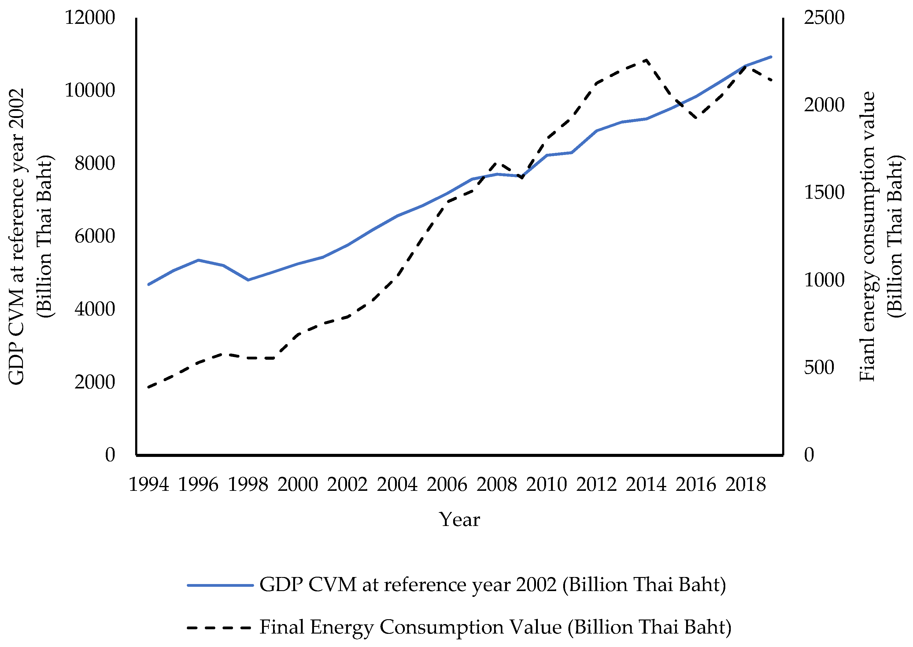
Figure 1. Thailand’s annual gross domestic product (GDP) chain volume measure (CVM) at reference year 2002 (primary vertical axis), and annual expenditure on final energy consumption (secondary vertical axis) during 1994–2019. Source: [1].
Energies 15 01578 g001
Figure 2. Annual expenditures (THB billion) on final energy consumption of petroleum products, natural gas, and coal/lignite in Thailand during 1994–2019. Source: [1].
Energies 15 01578 g002
Figure 3. Annual values of Thailand’s energy imports (THB billion) during 1994–2019. Source: [1].
Energies 15 01578 g003
Figure 4. Quarterly expenditure shares of petroleum products (wpt) (primary vertical axis), coal and lignite (wcl), and natural gas (wng) (secondary vertical axis) during 1993–2019.
Energies 15 01578 g004
Table 1. Summary of studies reporting the elasticities for energy-related commodities in Thailand.
StudySectorModelElasticitiesData
Own PriceIncome
[2]ManufacturingDynamic translogFuel oil −0.521
LPG −0.146
Electricity −0.301
Diesel 0.889
Coal and lignite 0.732
Annual
1979–1999
[3]Final oil consumption for seven sectorsDynamic panel and autoregressive distributed lagShort run −0.40 to −0.26
Long run −1.70 to −0.76
Panel
1981–2007
[4]Road transportLog-linear, cointegration and error correctionShort run/long run
Diesel −0.23/−0.53
Gasoline −0.14/−0.57
Short run/long run
Diesel 0.57/1.32Gasoline 0.35/1.40
Annual
1982–2008
[23]Final energy demandLog-log 0.923Annual
2008–2017
[24]TransportAIDSOctane 95 −1.08
Octane 91 −1.21
Diesel −0.17
Monthly
2011–2015
[25]TransportQAIDSUncompensated/compensatedgasoline −2.775/
−1.9296
LPG −0.8583/−0.5463
Diesel −1.018/−0.5474
Panel
Socio-economic survey (SES) in years 2009, 2013 and 2015
[26]TransportLog-linear GDP 0.995Annual
1989–2008
[27]Imported crude oilCointegrationShort run 0.042
Long run −0.066
Short run 0.484
Long run 0.997
Panel
2002–2011
Table 2. Estimates from the GQAIDS, GAIDS, QAIDS, and AIDS Models.
Model
ParameterGQAIDSGAIDSQAIDSAIDS
Objective Value1.8151.8201.8431.861
Adjust R 2 of Wcl0.6400.6380.6430.655
Adjust R 2 of Wng0.9890.9860.9880.983
λ 1 −0.002
(0.002)
n/a0.0002
(0.001)
n/a
λ 2 −0.014 ***
(0.002)
n/a−0.013 ***
(0.001)
n/a
λ 3 0.016 ***
(0.001)
n/a0.013 ***
(0.001)
n/a
c 1 571.06 ***
(79.932)
812.91 ***
(180.1)
n/an/a
c 2 160.19 ***
(59.351)
112.56
(116.9)
n/an/a
c 3 5121.60 ***
(13.109)
6278.51 ***
(391.9)
n/an/a
α 1 −0.181
(0.231)
0.165
(0.104)
0.054
(0.165)
−0.086 ***
(0.031)
α 2 −1.644 ***
(0.238)
0.313 *
(0.182)
−1.627 ***
(0.168)
0.157 *
(0.090)
α 3 2.825***
(0.334)
0.522**
(0.244)
2.573***
(0.235)
0.929 ***
(0.099)
β 1 0.045
(0.038)
−0.011
(0.011)
−0.002
(0.029)
0.016 ***
(0.003)
β 2 0.310 ***
(0.036)
−0.027
(0.021)
0.296 ***
(0.025)
−0.014
(0.010)
β 3 −0.355 ***
(0.041)
0.038
(0.027)
−0.294 ***
(0.029)
−0.002
(0.011)
γ 11 0.021
(0.017)
0.030 ***
(0.011)
0.021***
(0.003)
0.019 ***
(0.002)
γ 12 −0.067
(0.050)
−0.010
(0.010)
0.002
(0.042)
−0.003
(0.002)
γ 13 0.046
(0.065)
−0.020
(0.015)
−0.023
(0.040)
−0.016***
(0.003)
γ 22 −0.352 ***
(0.094)
0.137 ***
(0.019)
−0.386 ***
(0.067)
0.029 ***
(0.004)
γ 23 0.419 ***
(0.092)
−0.126 ***
(0.019)
0.384 ***
(0.061)
−0.026 ***
(0.005)
γ 33 −0.465 ***
(0.124)
0.147 ***
(0.026)
−0.361 ***
(0.079)
0.042 ***
(0.006)
AR(1) of Wcl0.376 ***
(0.095)
0.291 ***
(0.096)
0.338 ***
(0.093)
0.239 **
(0.092)
AR(2) of Wcl0.213 **
(0.104)
0.200 *
(0.103)
0.198 **
(0.100)
0.174 *
(0.096)
AR(3) of Wcl0.040
(0.103)
0.077
(0.101)
0.063
(0.100)
0.032
(0.095)
AR(4) of Wcl0.370 ***
(0.096)
0.411 ***
(0.097)
0.401 ***
(0.094)
0.344 ***
(0.093)
AR(1) of Wng0.965 ***
(0.107)
0.926 ***
(0.106)
0.943 ***
(0.105)
0.807 ***
(0.102)
AR(2) of Wng−0.117
(0.148)
−0.063
(0.144)
−0.245 *
(0.143)
0.018
(0.133)
AR(3) of Wng0.298 *
(0.176)
0.248 *
(0.145)
0.394 ***
(0.143)
0.088
(0.134)
AR(4) of Wng−0.135
(9.593)
−0.100
(0.107)
−0.080
(0.106)
0.102
(0.103)
Wald Test of the null: c 1 , c 2 , c 3 = 0 5.82 × 10⁹ ***1399.5 ***n/an/a
Notes: the values in parenthesis are standard errors. Subscripts 1, 2, 3 refer to coal and lignite, natural gas, and petroleum products, respectively. ***, **, * indicate that the estimate is statistically significant at the 1%, 5%, and 10% significance levels. AR(p) refers to the autoregressive process of lag order p.
Table 3. Average energy consumption and estimated pre-commitments from the GQAIDS and GAIDS models.
Average Consumption
(KTOE)
GQAIDSGAIDS
Energy SourcePre-Commitments
(KTOE)
Percentage of the Average ConsumptionPre-Commitments
(KTOE)
Percentage of the Average Consumption
Coal and Lignite1493.48571.0638.24%812.9154.43%
Natural Gas1069.81160.1914.97%112.5610.52%
Petroleum Products8001.175121.6064.01%6278.5178.47%
Table 4. Elasticities estimated from GQAIDS, GAIDS, QAIDS, and AIDS models.
ElasticitiesGQAIDSQAIDSGAIDSAIDS
Price ofPrice ofPrice ofPrice of
Coal and LigniteNatural GasPetroleum ProductsCoal and LigniteNatural GasPetroleum ProductsCoal and LigniteNatural GasPetroleum ProductsCoal and LigniteNatural GasPetroleum Products
Expenditure Elasticities
Expenditure Elasticities0.778 **
(0.343)
0.335 **
(0.146)
1.057 ***
(0.012)
1.117 ***
(0.138)
0.738 ***
(0.118)
1.018 ***
(0.010)
0.685
(0.484)
0.489 **
(0.224)
1.048 ***
(0.022)
1.609 ***
(0.131)
0.817 ***
(0.133)
0.998 ***
(0.012)
Uncompensated own-and cross-price
Coal and Lignite−0.069
(0.152)
−0.042
(0.188)
−0.717 **
(0.289)
−0.203 **
(0.093)
−0.193
(0.127)
−0.725 ***
(0.126)
−0.066
(0.182)
−0.172
(0.185)
−0.429
(0.539)
−0.284 ***
(0.087)
−0.148
(0.092)
−1.220 ***
(0.172)
Natural Gas−0.003
(0.058)
−0.125
(0.085)
−0.330 *
(0.166)
−0.055
(0.040)
−0.493 ***
(0.055)
−0.326 **
(0.142)
−0.053
(0.064)
−0.101
(0.100)
−0.320
(0.262)
−0.029
(0.031)
−0.612 ***
(0.055)
−0.163
(0.141)
Petroleum Products−0.026 ***
(0.007)
−0.081 ***
(0.006)
−0.956 ***
(0.014)
−0.017 ***
(0.004)
−0.047 ***
(0.006)
−0.955 ***
(0.012)
−0.021 ***
(0.007)
−0.068 ***
(0.008)
−0.964 ***
(0.026)
−0.017 ***
(0.003)
−0.027 ***
(0.005)
−0.954 ***
(0.013)
Compensated own- and cross-price
Coal and Lignite−0.049
(0.151)
0.018
(0.175)
0.053
(0.250)
−0.174 *
(0.093)
−0.107
(0.119)
0.370 **
(0.152)
−0.048
(0.181)
−0.120
(0.190)
0.247
(0.247)
−0.242 ***
(0.087)
−0.024
(0.090)
0.336 ***
(0.121)
Natural Gas0.006
(0.059)
−0.099
(0.086)
0.002
(0.077)
−0.036
(0.040)
−0.436 ***
(0.057)
0.397 ***
(0.075)
−0.040
(0.064)
−0.063
(0.103)
0.162
(0.108)
−0.008
(0.030)
−0.550 ***
(0.054)
0.627 ***
(0.062)
Petroleum Products0.001
(0.007)
0.0002
(0.006)
0.092 ***
(0.011)
0.010 **
(0.004)
0.031 ***
(0.006)
0.042 ***
(0.009)
0.006
(0.006)
0.013
(0.008)
0.070 ***
(0.015)
0.009 ***
(0.003)
0.050 ***
(0.005)
0.011
(0.011)
Allen own- and cross-price
Coal and Lignite−1.899
(5.842)
0.233
(2.274)
0.054
(0.253)
−6.761 *
(3.620)
−1.392
(1.550)
0.377 **
(0.155)
−1.866
(7.021)
−1.554
(2.466)
0.250
(0.250)
−9.397 ***
(3.388)
−0.310
(1.166)
0.347 ***
(0.125)
Natural Gas −1.285
(1.121)
0.002
(0.078)
−5.661 ***
(0.740)
0.405 ***
(0.074)
−0.821
(1.342)
0.164
(0.110)
−7.136 ***
(0.699)
0.649 ***
(0.063)
Petroleum Products 0.093 ***
(0.011)
0.043 ***
(0.009)
0.071 ***
(0.015)
0.011
(0.011)
Morishima
Coal and Lignite 0.083
(0.219)
0.238
(0.302)
0.300 **
(0.144)
0.231*
(0.130)
−0.072
(0.228)
0.535
(0.556)
0.465 ***
(0.107)
−0.265
(0.179)
Natural Gas0.066
(0.166)
0.626 ***
(0.179)
0.148
(0.106)
0.629 ***
(0.154)
0.013
(0.199)
0.643 **
(0.285)
0.255 ***
(0.094)
0.791 ***
(0.153)
Petroleum Products0.043
(0.156)
0.043
(0.089)
0.187 *
(0.095)
0.446 ***
(0.059)
0.045
(0.187)
0.033
(0.107)
0.267 ***
(0.089)
0.0585 ***
(0.059)
Notes: the values in parenthesis are standard errors. ***, **, * indicate that the estimate is statistically significant at the 1%, 5%, and 10% significance levels.
Publisher’s Note: MDPI stays neutral with regard to jurisdictional claims in published maps and institutional affiliations.